arX

iv:h

ep-p

h/01

0227

0v3

30

Sep

2001

FTUAM 01/03

IFT-UAM/CSIC-01-04

HIP-2000-69/TH

SUSX-TH/01-007

February 2001

Determination of the String Scale in D-Brane Scenarios and

Dark Matter Implications

D.G. Cerdeno1,2, E. Gabrielli3, S. Khalil4,5, C. Munoz1,2, E. Torrente-Lujan1

1 Departamento de Fısica Teorica C-XI, Universidad Autonoma de Madrid,

Cantoblanco, 28049 Madrid, Spain.

2 Instituto de Fısica Teorica C-XVI, Universidad Autonoma de Madrid,

Cantoblanco, 28049 Madrid, Spain.

3 Institute of Physics, University of Helsinki,

P.O. Box 9, Siltavuorenpenger 20 C, FIN-00014 Helsinki, Finland.

4 Centre for Theoretical Physics, University of Sussex, Brighton BN1 9QJ, U.K.

5 Ain Shams University, Faculty of Science, Cairo 11566, Egypt.

Abstract

We analyze different phenomenological aspects of D-brane constructions. First,

we obtain that scenarios with the gauge group and particle content of the su-

persymmetric standard model lead naturally to intermediate values for the

string scale, in order to reproduce the value of gauge couplings deduced from

experiments. Second, the soft terms, which turn out to be generically non uni-

versal, and Yukawa couplings of these scenarios are studied in detail. Finally,

using these soft terms and the string scale as the initial scale for their running,

we compute the neutralino-nucleon cross section. In particular we find regions

in the parameter space of D-brane scenarios with cross sections in the range of

10−6–10−5 pb, i.e. where current dark matter experiments are sensitive. For

instance, this can be obtained for tan β > 5.

PACS: 11.25.Mj, 12.10.Kt, 95.35.+d, 04.65.+e

Keywords: D-branes, string scale, soft terms, dark matter

1 Introduction

Although the standard model provides a correct description of the observable world,

there exist, however, strong indications that it is just an effective theory at low energy of

some fundamental one. The only candidates for such a theory are, nowadays, the string

theories, which have the potential to unify the strong and electroweak interactions with

gravitation in a consistent way.

In the late eighties, working in the context of the perturbative heterotic string, a

number of interesting four-dimensional vacua with particle content not far from that

of the supersymmetric standard model were found [1]. Supersymmetry breaking was

most of the times assumed to take place non-perturbatively by gaugino condensation

in a hidden sector of the theory. Until recently, it was thought that this was the only

way in order to construct realistic string models. However, in the late nineties, we have

discovered that explicit models with realistic properties can also be constructed using

D-brane configurations from type I string vacua [2]-[8]. Besides, it has been realized

that the string scale, MI , may be anywhere between the weak scale, MW , and the

Planck scale, MP lanck [9, 10, 3, 4, 11, 12]. This is to be compared to the perturbative

heterotic string where the relation MI =√

α8MP lanck, with α the gauge coupling, fixes

the value of the string scale.

The freedom to play with the value of MI is particularly interesting since there

are several arguments in favour of supersymmetric scenarios with scales MI ≈ 1010−14

GeV. First, these scales were suggested in [11] to explain many experimental observa-

tions as neutrino masses or the scale for axion physics. Second, with the string scale

of order 1010−12 GeV one is able to attack the hierarchy problem of unified theories

[12]. The mechanism is the following. In supergravity models supersymmetry can be

spontaneously broken in a hidden sector of the theory and the gravitino mass, which

sets the overall scale of the soft terms, is given by:

m3/2 ≈F

MP lanck, (1)

where F is the auxiliary field whose vacuum expectation value breaks supersymmetry.

Since in supergravity one would expect F ≈ M2P lanck, one obtains m3/2 ≈ MP lanck

and therefore the hierarchy problem solved in principle by supersymmetry would be

re-introduced, unless non-perturbative effects such as gaugino condensation produce

F ≈ MW MP lanck. However, if the scale of the fundamental theory is MI ≈ 1010−12 GeV

instead of MP lanck, then F ≈ M2I and one gets m3/2 ≈ MW in a natural way, without

invoking any hierarchically suppressed non-perturbative effect. Third, for intermediate

scale scenarios charge and color breaking constraints become less important. Let us

1

recall that charge and color breaking minima in supersymmetric theories might make

the standard vacuum unstable. Imposing that the standard vacuum should be the

global minimum the corresponding constraints turn out to be very strong and, in

fact, working with the usual unification scale MGUT ≈ 1016 GeV, there are extensive

regions in the parameter space of soft supersymmetry-breaking terms that become

forbidden [13]. For example, for the dilaton-dominated scenario of superstrings the

whole parameter space turns out to be excluded [14] on these grounds. The stability

of the corresponding constraints with respect to variations of the initial scale for the

running of the soft breaking terms was studied in [15], finding that the larger the

scale is, the stronger the bounds become. In particular, by taking MP lanck rather than

MGUT for the initial scale stronger constraints were obtained. Obviously the smaller the

scale is, the weaker the bounds become. In [16] intermediate scales rather than MGUT

were considered for the dilaton-dominated scenario with the interesting result that it

is allowed in a large region of parameter space. Finally, there are other arguments in

favour of scenarios with intermediate string scales MI ≈ 1010−14 GeV. For example

these scales might also explain the observed ultra-high energy (≈ 1020 eV) cosmic rays

as products of long-lived massive string mode decays. Besides, several models of chaotic

inflation favour also these scales [17].

In the present article we are going to analyze in detail whether or not those inter-

mediate string scales are also necessary in order to reproduce the low-energy data, i.e.

the values of the gauge couplings deduced from CERN e+e− collider LEP experiments.

In this sense, we will see that D-branes scenarios indeed lead naturally to intermediate

values for the string scale MI .

On the other hand, it has been noted that the neutralino-nucleon cross section is

quite sensitive to the value of the initial scale for the running of the soft breaking

terms [18]. The smaller the scale is, the larger the cross section becomes. In particular,

by taking 1010−12 GeV rather than 1016 GeV for the initial scale, the cross section

increases substantially σ ≈ 10−6–10−5 pb. This result is extremely interesting since the

lightest neutralino is usually the lightest supersymmetric particle (LSP), and therefore

a natural candidate for dark matter in supersymmetric theories [19], and current dark

matter detectors, DAMA [20] and CDMS [21], are sensitive to a neutralino-nucleon

cross section in the above range.

The initial scale for the running of the soft terms in D-brane scenarios is MI . As

mentioned above, several theoretical and phenomenological arguments suggest that

intermediate values for this scale are welcome. Thus it is natural to wonder how much

the standard neutralino-nucleon cross section analysis will get modified in D-brane

scenarios. This is another aim of this article.

2

The content of the article is as follows. In Section 2 we will try to determine the

string scale in D-brane scenarios imposing the experimental constraints on the values of

the gauge coupling constants. Although we will concentrate mainly in scenarios where

the SU(3)c, SU(2)L and U(1)Y groups of the standard model come from different sets

of Dp-branes, we will also review the scenario where they come from the same set of

Dp-branes. The fact that the U(1)Y group arises as a linear combination of different

U(1)’s, due to their D-brane origin, is crucial in the analysis.

In Section 3 we will use the results of Section 2, in particular the matter distribu-

tion due to the D-brane origin of the U(1) gauge groups, in order to derive the soft

supersymmetry breaking terms of the D-brane scenarios which may give rise to the

supersymmetric standard model. Generically they are non-universal. This analysis is

carried out under the assumption of dilaton/moduli supersymmetry breaking [27]-[30].

We emphasize that this assumption of dilaton/moduli dominance is more compelling

in the D-brane scenarios where only closed string fields like S and Ti can move into the

bulk and transmit supersymmetry breaking from one D-brane sector to some other.

Finally, we will also discuss the structure of Yukawa coupling matrices.

In Section 4, using the soft terms of the D-brane scenarios previously studied, we

compute the neutralino-nucleon cross section. We will see how the compatibility of

regions in the parameter space of these scenarios with the sensitivity of current dark

matter experiments depends not only on the value of the string scale but also on the

non-universality of the soft terms.

Finally, the conclusions are left for Section 5.

2 D-brane scenarios and the string scale

As mentioned in the Introduction there exists the interesting possibility that the su-

persymmetric standard model might be built using D-brane configurations. In this

case there are two possible avenues to carry it out: i) The SU(3)c, SU(2)L and U(1)Y

groups of the standard model come from different sets of Dp-branes. ii) They come

from the same set of Dp-branes.

Since the two scenarios are interesting and qualitatively different, we will discuss

both separately. We will see in detail below that the first one (i), in order to reproduce

the values of the gauge couplings deduced from CERN e+e− collider LEP experiments,

leads naturally to intermediate values for the string scale MI . One realizes that this is

an interesting result since there are several arguments in favour of intermediate scales,

as discussed in the Introduction. This approach was used first in [31] for the case

3

of non-supersymmetric Dp-branes with the result of a string scale of the order of a

few TeV. In any case, it is worth remarking the difficulty of obtaining three copies of

quarks and leptons if the gauge groups are attached to different sets of Dp-branes1.

Thus whether or not the scenarios discussed below, may arise from different sets of Dp-

branes in explicit string constructions is an important issue which is worth attacking

in the future.

Concerning the other scenario (ii), models with the gauge group of the standard

model and three families of particles have been explicitly built [6, 7]. We will review

whether or not intermediate scales arise naturally.

2.1 Embedding the gauge groups within different sets of Dp-

branes

It is a plausible situation to assume that the SU(3)c and the SU(2)L groups of the

standard model could come from different sets of Dp-branes [32, 3]. By different sets

we mean Dp-branes whose world-volume is not identical. In particular, notice that

the standard model contains particles (the left-handed quarks Qu) transforming both

under SU(3)c and SU(2)L. That means that there must be some overlap of the world-

volumes of both sets of Dp-branes. Thus e.g., one cannot put SU(3)c inside a set of

D3-branes and SU(2)L within another set of parallel D3-branes on a different point

of the compact space since then there would be no massless modes corresponding to

the exchange of open strings between both sets of branes which could give rise to the

left-handed quarks.

Thus we need to embed SU(3)c inside D-branes, say Dp3-branes, and SU(2)L within

other D-branes, say Dp2-branes, in such a way that their corresponding world-volumes

have some overlap. Since we are working in general with type IIB orientifolds, pN

can be 3, 5i, 7i, and 9, where the index i = 1, 2, 3 denotes what complex compact

coordinate is included in the D5-brane world-volume, or is transverse to the D7-brane

world-volume. Not all types of DpN -branes may be present simultaneously if we want

to preserve N = 1 in D = 4. For a given D = 4, N = 1 vacuum we can have at most

either D9-branes with D5i-branes or D3-branes with D7i-branes.

In type IIB orientifold models, and in general on the world-volume of D-branes,

SU(N) groups come along with a U(1) factor, say U(1)N , so that indeed we are dealing

with U(N) groups, in which both SU(N) and U(1)N share the same coupling constant,

αN . Thus U(1)Y might be a linear combination of two U(1) gauge groups arising from

U(3)c and U(2)L within Dp3- and Dp2-branes respectively [33]. Although this is the

1 We thank L.E. Ibanez for discussions about this point (see also [6])

4

3Dp1Dp Dp2

wb

g

Dqce

Q

L,

U(1)U(3) U(2) Lc

u

cd

eH1

H2

uc

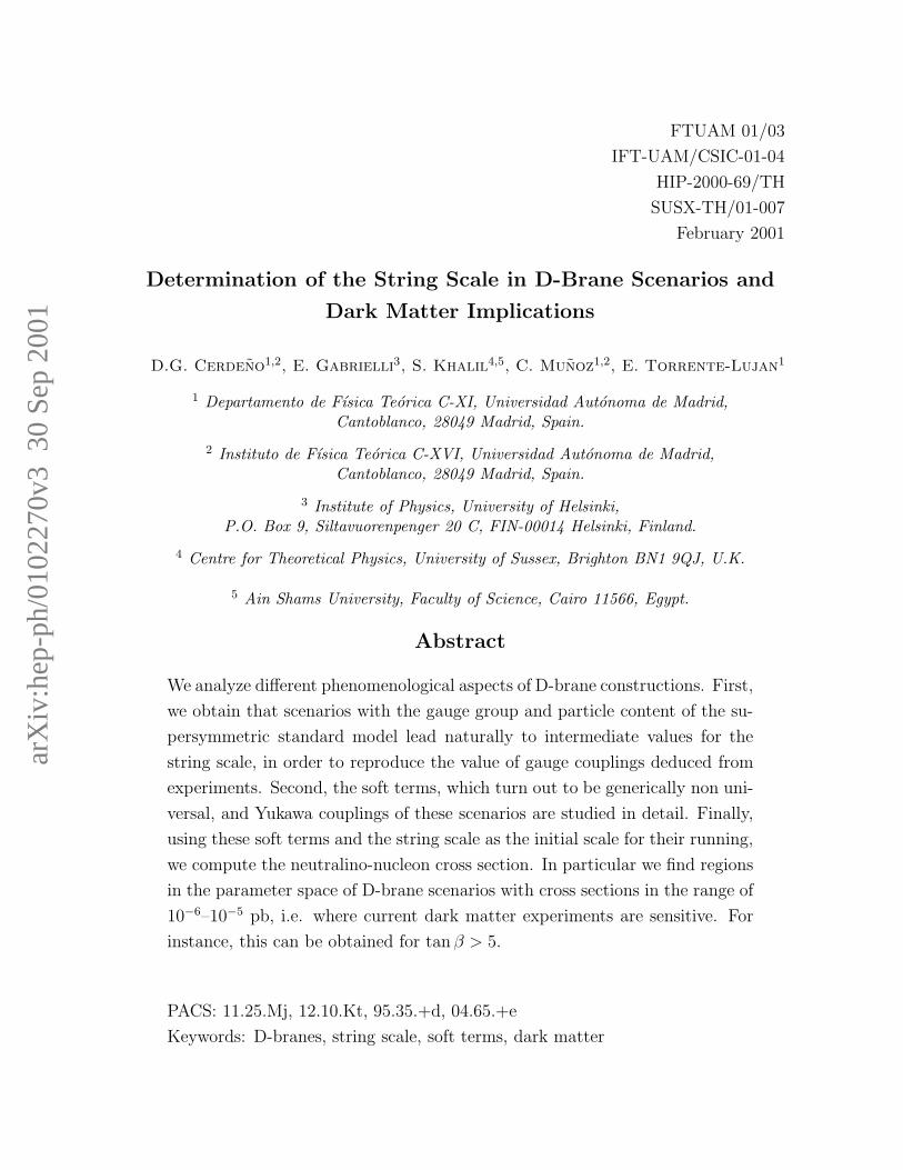
Figure 1: A generic D-brane scenario giving rise to the gauge bosons and matter of

the standard model. It contains three Dp3-branes, two Dp2-branes and one Dp1-brane,

where pN may be either 9 and 5i or 3 and 7i. The presence of extra D-branes, say

Dq-branes, is also necessary as explained in the text. For each set the DpN -branes are

in fact on the top of each other.

simplest possibility, its analysis is somehow subtle [31] and we prefer to carry it out at

the end of this subsection. Thus we will analyze first a more general case, where an

extra U(1) arising from another D-brane, say Dp1-brane, contributes to the combination

giving rise to the correct hypercharge of the standard model matter [31, 6]. This is

schematically shown in Fig. 1, where open strings starting and ending on the same sets

of DpN -branes give rise to the gauge bosons of the standard model. For the sake of

visualization each set is depicted at parallel locations, but in fact they are intersecting

each other as discussed above.

In [6] a Z3 orientifold model with U(3)c × U(2)L × U(1) observable gauge group,

and therefore giving rise to SU(3)c × SU(2)L × U(1)3 × U(1)2 × U(1)1 as discussed

above, was explicitly built. Nevertheless, this model is embedded in D3-branes, i.e.

p3 = p2 = p1 = 3, and therefore we will discuss it in detail in Subsection 2.2.

On the other hand, in [31] the existence of standard models coming from different

sets of non-supersymmetric Dp-branes was assumed and several consequences were

discussed. In particular, imposing Dp3=Dp1, i.e. α3 = α1, the low-energy data are

reproduced for a string scale of the order of a few TeV. Here we will carry out the general

analysis of supersymmetric Dp-branes with the interesting result that intermediate

5

Matter Fields Q3 Q2 Q1 Q2 Q1 Q2 Q1 Q2 Q1 Y

Qu(3, 2) 1 -1 0 1 0 1 0 -1 0 1/6

uc(3, 1) -1 0 -1 0 -1 0 0 0 0 -2/3

dc(3, 1) -1 0 0 0 0 0 1 0 1 1/3

Le(1, 2) 0 1 0 1 -1 1 0 1 -1 -1/2

ec(1, 1) 0 0 1 0 1 0 1 0 1 1

Table 1: The four possible assignments of quantum numbers (multiplied by√

2N) of

a family of quarks and leptons of the standard model under U(1)3 × U(1)2 × U(1)1.

Note that Q3 is always fixed. The usual hypercharge Y is given in the last column.

values (≈ 1010−12 GeV) for the string scale may arise in a natural way.

2.1.1 General scenario with Dp3 6= Dp2 6= Dp1 6= Dp3

Let us denote by Q3, Q2 and Q1 the charges of U(1)3, U(1)2, and U(1)1 respectively.

Following then the analysis of Antoniadis, Kiritsis and Tomaras [31] a family of quarks

and leptons can have the four assignments of quantum numbers given in Table 1, in

order to obtain the hypercharge of the standard model

Y = c3

√6Q3 + c2

√4Q2 +

√2Q1 , (2)

where c3 = −1/3, c2 = −1/2 (c2 = 1/2) for the first (second) assignment and c3 = 2/3,

c2 = −1/2 (c2 = 1/2) for the third (fourth) assignment. Note that U(N) generators

are normalized as Tr T aT b = 12δab, and therefore the fundamental representation of

SU(N) has QN = 1/√

2N .

For example, as discussed above, the quark doublet Qu always arises from an open

string with one end on Dp3-branes and the other end on Dp2-branes. In the first

assignment of Table 1 Qu transforms as a 2 under U(2) and therefore Q2 = −1/√

4.

uc (dc) arises from an open string with one end on Dp3-branes and the other end on

Dp1 (Dq)-branes2 with Q1 = −1/√

2 (0). Finally, in the case of leptons, Le (ec) arises

from an open string with one end on Dp2 (Dp1)-branes and the other end on Dq-branes

with Q1 = 0 (1/√

2). This is schematically shown in Fig. 1. The other three possible

2As we see from here the presence of extra D-branes, say Dq-branes, is necessary in order to

reproduce the correct hypercharge for the matter. In addition, in Subsection 2.2 we will see an

explicit model where Dq-branes are also necessary to cancel non-vanishing tadpoles. The additional

U(1) factors associated to the Dq-branes will be anomalous and therefore with a mass of the order of

the string scale.

6

assignments can also be analyzed similarly. Let us remark that other scenarios with

uc, dc (ec) arising from open strings with both ends on Dp3 (Dp2)-branes are possible,

since these particles can be obtained as the antisymmetric product of two triplets of

SU(3) (doublets of SU(2)). However, these scenarios do not give rise to a modification

of the analysis of the string scale [31], and therefore we will not consider them here.

Concerning the possible quantum numbers of Higgses, they will be discussed in

in Section 3 where they are important e.g. in order to determine whether or not all

Yukawa couplings in D-brane scenarios are allowed.

Let us now try to determine the type I string scale MI , using the above information.

On the one hand, from (2) one obtains the following relation at MI :

1

αY (MI)=

2

α1(MI)+

4c22

α2(MI)+

6c23

α3(MI). (3)

On the other hand, the usual RGE’s for gauge couplings are given by

1

αj(MI)=

1

αj(MZ)+

bnsj

2πln

Ms

MZ+

bsj

2πln

MI

Ms, (4)

where bsj (bns

j ) with j = 2, 3, Y are the coefficients of the supersymmetric (non-supersym-

metric) β-functions, and the scale Ms corresponds to the supersymmetric threshold,

200 GeV <∼ Ms <∼ 1000 GeV. Thus using (3), (4) and the fact that always c22 = 1/4

one can compute MI with the result

lnMI

Ms

=2π(

1αY (MZ )

− 2α1(MI)

− 1α2(MZ )

− 6c23

α3(MZ)

)

+ (bnsY − bns

2 − 6c23b

ns3 ) ln Ms

MZ

(6c23b

s3 + bs

2 − bsY )

. (5)

Using the experimental values [34] MZ = 91.1870 GeV, α3(MZ) = 0.1184, α2(MZ) =

0.0338, αY (MZ) = 0.01016, and the matter content of the minimal supersymmetric

standard model (MSSM), i.e. bs3 = 3, bs

2 = −1, bsY = −11 and bns

3 = 7, bns2 = 19/6,

bnsY = −41/6, one obtains for c3 = −1/3

lnMI

Ms= 33.09 − 1.05

α1(MI)− 1.22 ln

Ms

MZ. (6)

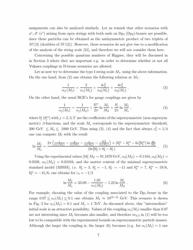
For example, choosing the value of the coupling associated to the Dp1-brane in the

range 0.07 <∼ α1(MI) <∼ 0.1 one obtains MI ≈ 1010−12 GeV. This scenario is shown

in Fig. 2 for α1(MI) = 0.1 and Ms = 1 TeV. As discussed above, this ”intermediate”

initial scale is an attractive possibility. Values of the coupling α1(MI) smaller than 0.07

are not interesting since MI becomes also smaller, and therefore m3/2 in (1) will be too

low to be compatible with the experimental bounds on supersymmetric particle masses.

Although the larger the coupling is, the larger MI becomes (e.g. for α1(MI) = 1 one

7

Figure 2: Running of the gauge couplings of the MSSM with energy Q embedding the

gauge groups within different sets of Dp-branes (solid lines). Due to the D-brane origin

of the U(1) gauge groups, relation (3) must be fulfilled. For comparison the running

of the MSSM couplings with the usual normalization factor for the hypercharge, 3/5,

is also shown with dashed lines.

is even able to obtain MI ≈ 5 × 1015 GeV), one should be careful with the range of

validity of the perturbative regime.

On the other hand, the case c3 = 2/3 is less interesting since one obtains the upper

bound MI ≈ 3 × 108 GeV.

It is worth noticing that non-supersymmetric scenarios can also be analyzed with

the above formula (5) with the substitutions Ms → MZ , bsi → bns

i . For example,

MI ≈ 1 TeV can be obtained with α1(MI) ≈ 0.035 for c3 = −1/3, and α1(MI) ≈ 0.056

for c3 = 2/3.

2.1.2 Scenarios with Dp1=Dp3 or Dp1=Dp2

Let us now simplify the above analysis assuming that the D-brane associated to the

U(1)1 is on top of one of the other D-branes. In this case we have two possibilities, either

Dp1=Dp3 or Dp1=Dp2. Let us start analyzing the possibility Dp1=Dp3, which implies

α1 = α3. Then eq.(5) is still valid with the substitutions 2α1(MI )

+6c2

3

α3(MZ )→ 2+6c2

3

α3(MZ),

6c23b

s,ns3 → (2 + 6c2

3)bs,ns3 . As a consequence, for c3 = −1/3, one obtains the following

prediction: MI ≈ 6× 108 GeV, with Ms = 200 GeV. A slightly low value to be able to

obtain m3/2 ≈ MW , as discussed below eq.(1). Obviously, the larger Ms is, the smaller

8

MI becomes. The case c3 = 2/3 is much worse since MI ≈ 100 TeV.

The other scenario Dp1=Dp2, which implies α1 = α2, does not improve the above

situation. One can use again eq.(5), but now with the substitutions 2α1(MI )

+ 1α2(MZ)

→3

α2(MZ ), bs,ns

2 → 3bs,ns2 . In particular, for c3 = −1/3, MI ≈ 500 GeV, with Ms = 200

GeV, whereas ln MI

Msis even negative for c3 = 2/3.

On the other hand, extra particles appear quite frecuently in superstring theories.

Since their presence will modify the denominator in (5), one might obtain larger values

for MI . For example, for Dp1=Dp3, and restricting ourselves to the case of singlets,

SU(2) doublets and colour triplets, one has

(2 + 6c23)b

s3 + bs

2 − bsY = 18 − 1

2(2 + 6c2

3)n3 −1

2n2 + q , (7)

where q =∑n1

i=1 Y 2i + 2

∑n2

j=1 Y 2J + 3

∑n3

k=1 Y 2k and n1,2,3 is the number of extra singlets,

doublets and triplets that the model under consideration has. Extra (3, 2) represen-

tations under SU(3) × SU(2) must be introduced in the formula for q just as two

triplets each. For instance, assuming the presence of two copies of dc+dc for the case

c3 = −1/3, one obtains MI ≈ 4 × 1010 GeV (≈ 8 × 109 GeV), with Ms = 200 GeV

(1 TeV). Concerning the running of the couplings, this scenario is similar to the one

shown in Fig. 2.

As above, we can also analyze non-supersymmetric scenarios. A string scale of

order a few TeV can be obtained without extra particles. In particular, for α1 = α2,

c3 = −1/3 and α1 = α3, c3 = 2/3 we recover the results of [31], MI ≈ 300 GeV and

MI ≈ 7 TeV, respectively.

2.1.3 Scenario without Dp1-brane

Let us finally consider the scenario where the U(1)Y is only a linear combination of

the two U(1) gauge groups arising from U(3)c and U(2)L within Dp3- and Dp2-branes

respectively [33].

As discussed in [31], there is only one assignment of quantum numbers for quarks

and leptons, in order to obtain the hypercharge of the standard model. The latter is

given by eq. (2) with c3 = −1/3, c2 = −1/2, Q1 = 0, i.e. Y = −13

√6Q3 − 1

2

√4Q2.

Whereas the charges Q3 and Q2 for Qu, dc and Le are as in the first assignment given

in Table 1, Q3 = 2/√

6, 0 and Q2 = 0,−2/√

4 for uc, ec. Clearly, uc and ec must arise

from open strings with both ends on Dp3-branes and Dp2-branes, respectively. As men-

tioned above, this is possible since these particles can be obtained as the antisymmetric

product of two triplets of SU(3) and doublets of SU(2), respectively.

9

With the above hypercharge, instead of eq. (3) one obtains 1αY (MI )

= 1α2(MI )

+ 2/3α3(MI)

,

and therefore eq. (5) is still valid with c3 = −1/3 and the substitution 2α1(MI)

→ 0.

As a consequence one can predict the string scale. For example, for Ms = 200 GeV

(Ms = 1 TeV) one obtains MI ≈ 1.8 × 1016 GeV (MI ≈ 1016 GeV). On the other

hand, a non-supersymmetric scenario [31] gives rise to a string scale which is too large,

MI ≈ 5 × 1013 GeV.

It is worth noticing [6] that for α3 = α2 one obtains the standard GUT normalization

for couplings αY = 35α2, and therefore MI ≈ 2 × 1016 GeV.

We thus conclude that, concerning the string scale MI , the generic models analyzed

above are very interesting from the point of view of their predictivity. Besides, the

values obtained for MI can be accomodated in type I strings, choosing the appropriate

values of the moduli. For instance, for the example studied below eq. (7) the experi-

mental values of couplings are obtained with MI ≈ 8 × 109 GeV for the case Ms = 1

TeV, and therefore the ratio α3(MI )α2(MI )

≈ 2. Let us assume that SU(3)c is embedded inside

D9-branes and SU(2)L inside D51-branes. Then one has the following relationships

M1M2M3

M2I

=α3MP lanck√

2,

M1M2I

M2M3

=α2MP lanck√

2, (8)

where Mi, i = 1, 2, 3, are the compactification masses associated to the compact radii

Ri. ChoosingM4

I

M2

2M2

3

≈ 1/2 one is able to reproduce the above ratio.

2.2 Embedding all gauge groups within the same set of Dp-

branes

The fact that to obtain three copies of quark and leptons is difficult, when gauge groups

come from different sets of DpN -branes, as mentioned above, is one of the motivations

in [6] to embed all gauge interactions in the same set of DpN -branes (p3 = p2 = p1 in

the notation above).

Here we will briefly review the results of Aldazabal, Ibanez, Quevedo and Uranga

[6] concerning this issue. They are able to build Z3 orientifold models with the gauge

group SU(3)c × SU(2)L × U(1)3 × U(1)2 × U(1)1 embedded in D3-branes, with no

additional non-abelian factors. They also argue that in the Z3 orientifold, which leads

naturally to three families, only the combination

Y = −1

3

√6Q3 −

1

2

√4Q2 +

√2Q1 (9)

will be non-anomalous. It is worth noticing that this is precisely the hypercharge given

in (2) with c3 = −1/3 and c2 = −1/2, i.e. the first assignment of Table 1. Likewise

10

Fig. 1 with Dp3=Dp2=Dp1=D3, and all D3-branes on top of each other, is also valid

as a schematic representation of this type of models. Dq-branes in the figure are now

D7-branes, which must be introduced in order to cancel non-vanishing tadpoles. Since

α3 = α2 = α1 = α, instead of (3) one obtains

1

αY (MI)=

11/3

α(MI), (10)

which is not the standard GUT normalization for couplings. This is due to the D-brane

origin of the U(1) gauge groups.

A model with all these properties was explicitly built in [6]. Although extra U(1)′s

on the D7-branes are present, they are anomalous and therefore the associated gauge

bosons have masses of the order of MI . In addition to D7-branes, anti-D7-branes

trapped at different Z3 fixed points are also present. Since they break supersymmetry

at the string scale MI , they can be used as the hidden sector of supergravity theories.

Thus this is an example of gravity mediated supersymmetry breaking.

On the other hand, in this model not only quarks and leptons come in three gener-

ations but also Higgses, i.e. it contains two pairs of extra doublets with respect to the

MSSM. In addition, three pairs of extra colour triplets are also present. Unfortunately,

this matter content cannot give rise to the correct values for αj(MZ). Although gener-

ically the extra triplets will be heavy, this does not modify the previous result. One

cannot exclude, however, the possibility that other models with the necessary matter

content, in order to reproduce the experimental values of couplings, might be built.

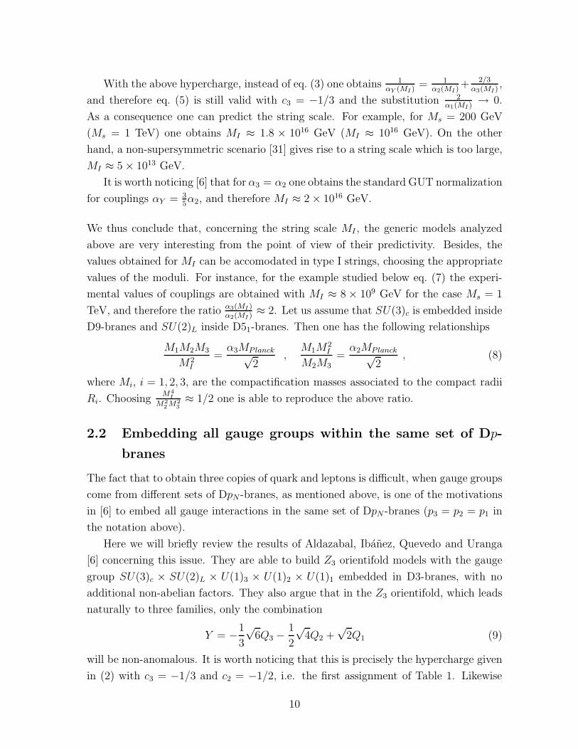
For example, if besides the matter content of the MSSM, we have six copies of H1+H2

and two copies of dc+dc unification at around MI = 1010 GeV, with α(MI) ≈ 1/14, is

obtained. This scenario is shown in Fig. 3 for Ms = 1 TeV.

It is worth noticing that these values can be accomodated in type I strings, choosing

the appropriate values of the moduli. For example, with an isotropic compact space,

the string scale is given by:

M4I =

αMP lanck√2

M3c , (11)

where Mc is the compactification scale. Thus one gets MI ≈ 1010−12 GeV with Mc ≈108−10 GeV.

Let us finally mention that another model with the gauge group of the standard

model and three families has recently been built [7]. The presence of additional Higgs

doublets and vector-like states allows an unification scale at an intermediate value.

11

Figure 3: Running of the gauge couplings with energy Q embedding all gauge groups

within the same set of D3-branes (solid lines). In addition to the matter content of

the MSSM, extra Higgs doublets and vector-like states are also present. Due to the

D-brane origin of the U(1) gauge groups, the normalization factor of the hypercharge

is 3/11 (see eq. (10)). For comparison the running of the MSSM couplings with the

usual normalization factor for the hypercharge, 3/5, is also shown with dashed lines.

3 Soft terms and Yukawa couplings in D-brane sce-

narios

General formulas for the soft supersymmetry-breaking terms in D-brane constructions

were obtained in [33], under the assumption of dilaton/moduli supersymmetry breaking

[27]-[30], using the parametrization introduced in [30]. On the other hand, general

Yukawa couplings in D-brane constructions have been studied in [35, 33]. Since we

need to use these results to obtain the soft terms and Yukawa couplings associated to

the D-brane scenarios discussed above, we summarize them in the Appendix A.

3.1 Embedding the gauge groups within different sets of Dp-

branes

3.1.1 General scenario with Dp3 6= Dp2 6= Dp1 6= Dp3

For the sake of concreteness, let us assume the following distribution of D-branes in

the scenario proposed in Subsection 2.1. Dp3-branes are D9-branes, Dp1-branes are

12

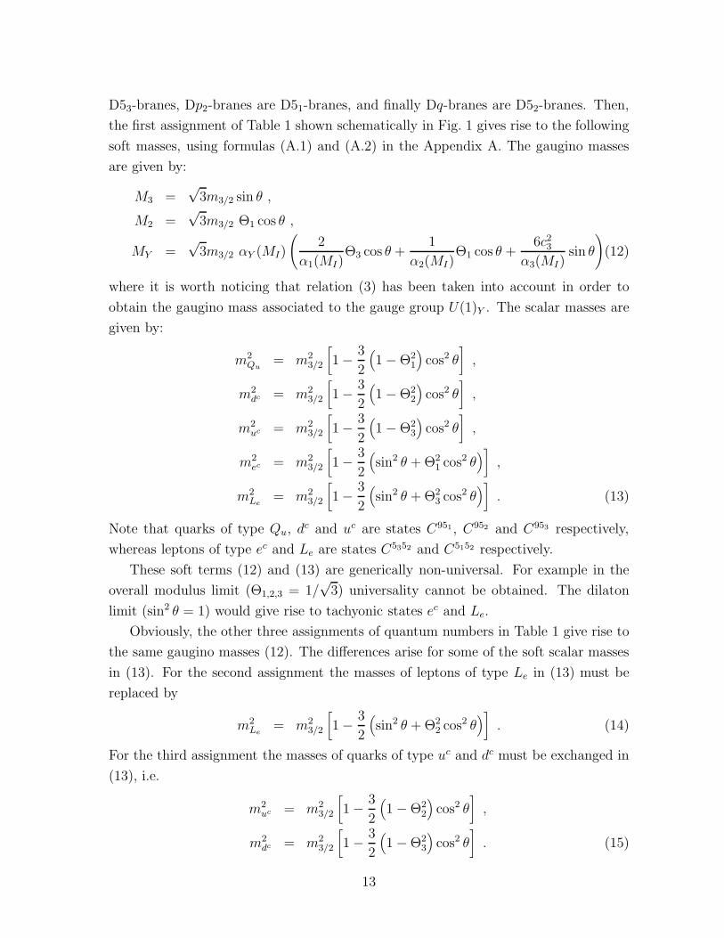
D53-branes, Dp2-branes are D51-branes, and finally Dq-branes are D52-branes. Then,

the first assignment of Table 1 shown schematically in Fig. 1 gives rise to the following

soft masses, using formulas (A.1) and (A.2) in the Appendix A. The gaugino masses

are given by:

M3 =√

3m3/2 sin θ ,

M2 =√

3m3/2 Θ1 cos θ ,

MY =√

3m3/2 αY (MI)

(

2

α1(MI)Θ3 cos θ +

1

α2(MI)Θ1 cos θ +

6c23

α3(MI)sin θ

)

(12)

where it is worth noticing that relation (3) has been taken into account in order to

obtain the gaugino mass associated to the gauge group U(1)Y . The scalar masses are

given by:

m2Qu

= m23/2

[

1 − 3

2

(

1 − Θ21

)

cos2 θ]

,

m2dc = m2

3/2

[

1 − 3

2

(

1 − Θ22

)

cos2 θ]

,

m2uc = m2

3/2

[

1 − 3

2

(

1 − Θ23

)

cos2 θ]

,

m2ec = m2

3/2

[

1 − 3

2

(

sin2 θ + Θ21 cos2 θ

)

]

,

m2Le

= m23/2

[

1 − 3

2

(

sin2 θ + Θ23 cos2 θ

)

]

. (13)

Note that quarks of type Qu, dc and uc are states C951 , C952 and C953 respectively,

whereas leptons of type ec and Le are states C5352 and C5152 respectively.

These soft terms (12) and (13) are generically non-universal. For example in the

overall modulus limit (Θ1,2,3 = 1/√

3) universality cannot be obtained. The dilaton

limit (sin2 θ = 1) would give rise to tachyonic states ec and Le.

Obviously, the other three assignments of quantum numbers in Table 1 give rise to

the same gaugino masses (12). The differences arise for some of the soft scalar masses

in (13). For the second assignment the masses of leptons of type Le in (13) must be

replaced by

m2Le

= m23/2

[

1 − 3

2

(

sin2 θ + Θ22 cos2 θ

)

]

. (14)

For the third assignment the masses of quarks of type uc and dc must be exchanged in

(13), i.e.

m2uc = m2

3/2

[

1 − 3

2

(

1 − Θ22

)

cos2 θ]

,

m2dc = m2

3/2

[

1 − 3

2

(

1 − Θ23

)

cos2 θ]

. (15)

13

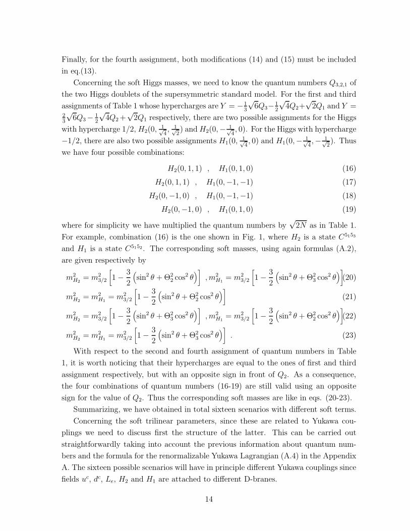
Finally, for the fourth assignment, both modifications (14) and (15) must be included

in eq.(13).

Concerning the soft Higgs masses, we need to know the quantum numbers Q3,2,1 of

the two Higgs doublets of the supersymmetric standard model. For the first and third

assignments of Table 1 whose hypercharges are Y = −13

√6Q3− 1

2

√4Q2+

√2Q1 and Y =

23

√6Q3− 1

2

√4Q2 +

√2Q1 respectively, there are two possible assignments for the Higgs

with hypercharge 1/2, H2(0,1√4, 1√

2) and H2(0,− 1√

4, 0). For the Higgs with hypercharge

−1/2, there are also two possible assignments H1(0,1√4, 0) and H1(0,− 1√

4,− 1√

2). Thus

we have four possible combinations:

H2(0, 1, 1) , H1(0, 1, 0) (16)

H2(0, 1, 1) , H1(0,−1,−1) (17)

H2(0,−1, 0) , H1(0,−1,−1) (18)

H2(0,−1, 0) , H1(0, 1, 0) (19)

where for simplicity we have multiplied the quantum numbers by√

2N as in Table 1.

For example, combination (16) is the one shown in Fig. 1, where H2 is a state C5153

and H1 is a state C5152 . The corresponding soft masses, using again formulas (A.2),

are given respectively by

m2H2

= m23/2

[

1 − 3

2

(

sin2 θ + Θ22 cos2 θ

)

]

, m2H1

= m23/2

[

1 − 3

2

(

sin2 θ + Θ23 cos2 θ

)

]

(20)

m2H2

= m2H1

= m23/2

[

1 − 3

2

(

sin2 θ + Θ22 cos2 θ

)

]

(21)

m2H2

= m23/2

[

1 − 3

2

(

sin2 θ + Θ23 cos2 θ

)

]

, m2H1

= m23/2

[

1 − 3

2

(

sin2 θ + Θ22 cos2 θ

)

]

(22)

m2H2

= m2H1

= m23/2

[

1 − 3

2

(

sin2 θ + Θ23 cos2 θ

)

]

. (23)

With respect to the second and fourth assignment of quantum numbers in Table

1, it is worth noticing that their hypercharges are equal to the ones of first and third

assignment respectively, but with an opposite sign in front of Q2. As a consequence,

the four combinations of quantum numbers (16-19) are still valid using an opposite

sign for the value of Q2. Thus the corresponding soft masses are like in eqs. (20-23).

Summarizing, we have obtained in total sixteen scenarios with different soft terms.

Concerning the soft trilinear parameters, since these are related to Yukawa cou-

plings we need to discuss first the structure of the latter. This can be carried out

straightforwardly taking into account the previous information about quantum num-

bers and the formula for the renormalizable Yukawa Lagrangian (A.4) in the Appendix

A. The sixteen possible scenarios will have in principle different Yukawa couplings since

fields uc, dc, Le, H2 and H1 are attached to different D-branes.

14

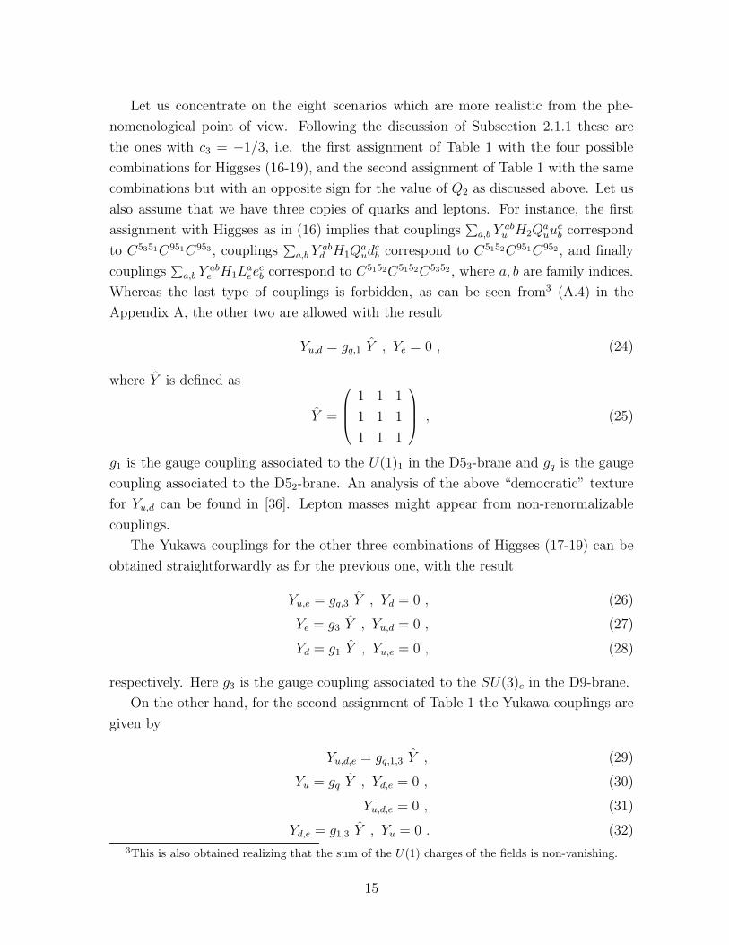
Let us concentrate on the eight scenarios which are more realistic from the phe-

nomenological point of view. Following the discussion of Subsection 2.1.1 these are

the ones with c3 = −1/3, i.e. the first assignment of Table 1 with the four possible

combinations for Higgses (16-19), and the second assignment of Table 1 with the same

combinations but with an opposite sign for the value of Q2 as discussed above. Let us

also assume that we have three copies of quarks and leptons. For instance, the first

assignment with Higgses as in (16) implies that couplings∑

a,b Y abu H2Q

auu

cb correspond

to C5351C951C953 , couplings∑

a,b Y abd H1Q

aud

cb correspond to C5152C951C952 , and finally

couplings∑

a,b Y abe H1L

aee

cb correspond to C5152C5152C5352 , where a, b are family indices.

Whereas the last type of couplings is forbidden, as can be seen from3 (A.4) in the

Appendix A, the other two are allowed with the result

Yu,d = gq,1 Y , Ye = 0 , (24)

where Y is defined as

Y =

1 1 1

1 1 1

1 1 1

, (25)

g1 is the gauge coupling associated to the U(1)1 in the D53-brane and gq is the gauge

coupling associated to the D52-brane. An analysis of the above “democratic” texture

for Yu,d can be found in [36]. Lepton masses might appear from non-renormalizable

couplings.

The Yukawa couplings for the other three combinations of Higgses (17-19) can be

obtained straightforwardly as for the previous one, with the result

Yu,e = gq,3 Y , Yd = 0 , (26)

Ye = g3 Y , Yu,d = 0 , (27)

Yd = g1 Y , Yu,e = 0 , (28)

respectively. Here g3 is the gauge coupling associated to the SU(3)c in the D9-brane.

On the other hand, for the second assignment of Table 1 the Yukawa couplings are

given by

Yu,d,e = gq,1,3 Y , (29)

Yu = gq Y , Yd,e = 0 , (30)

Yu,d,e = 0 , (31)

Yd,e = g1,3 Y , Yu = 0 . (32)

3This is also obtained realizing that the sum of the U(1) charges of the fields is non-vanishing.

15

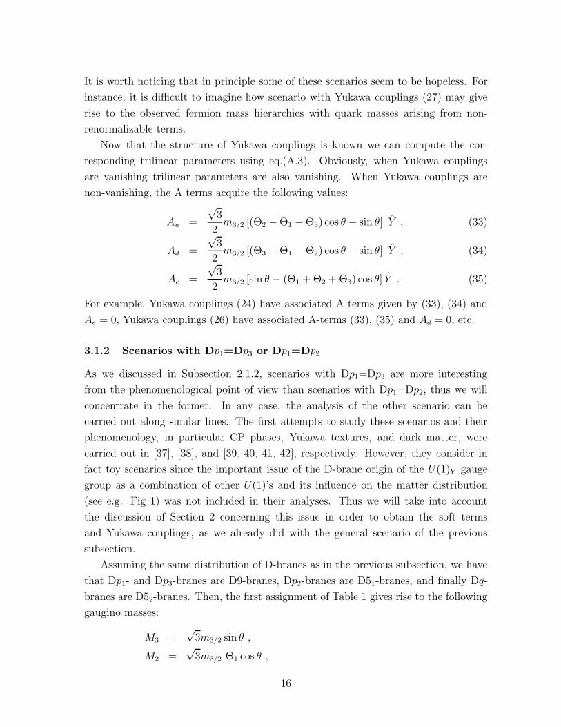
It is worth noticing that in principle some of these scenarios seem to be hopeless. For

instance, it is difficult to imagine how scenario with Yukawa couplings (27) may give

rise to the observed fermion mass hierarchies with quark masses arising from non-

renormalizable terms.

Now that the structure of Yukawa couplings is known we can compute the cor-

responding trilinear parameters using eq.(A.3). Obviously, when Yukawa couplings

are vanishing trilinear parameters are also vanishing. When Yukawa couplings are

non-vanishing, the A terms acquire the following values:

Au =

√3

2m3/2 [(Θ2 − Θ1 − Θ3) cos θ − sin θ] Y , (33)

Ad =

√3

2m3/2 [(Θ3 − Θ1 − Θ2) cos θ − sin θ] Y , (34)

Ae =

√3

2m3/2 [sin θ − (Θ1 + Θ2 + Θ3) cos θ] Y . (35)

For example, Yukawa couplings (24) have associated A terms given by (33), (34) and

Ae = 0, Yukawa couplings (26) have associated A-terms (33), (35) and Ad = 0, etc.

3.1.2 Scenarios with Dp1=Dp3 or Dp1=Dp2

As we discussed in Subsection 2.1.2, scenarios with Dp1=Dp3 are more interesting

from the phenomenological point of view than scenarios with Dp1=Dp2, thus we will

concentrate in the former. In any case, the analysis of the other scenario can be

carried out along similar lines. The first attempts to study these scenarios and their

phenomenology, in particular CP phases, Yukawa textures, and dark matter, were

carried out in [37], [38], and [39, 40, 41, 42], respectively. However, they consider in

fact toy scenarios since the important issue of the D-brane origin of the U(1)Y gauge

group as a combination of other U(1)’s and its influence on the matter distribution

(see e.g. Fig 1) was not included in their analyses. Thus we will take into account

the discussion of Section 2 concerning this issue in order to obtain the soft terms

and Yukawa couplings, as we already did with the general scenario of the previous

subsection.

Assuming the same distribution of D-branes as in the previous subsection, we have

that Dp1- and Dp3-branes are D9-branes, Dp2-branes are D51-branes, and finally Dq-

branes are D52-branes. Then, the first assignment of Table 1 gives rise to the following

gaugino masses:

M3 =√

3m3/2 sin θ ,

M2 =√

3m3/2 Θ1 cos θ ,

16

MY =√

3m3/2 αY (MI)

(

1

α2(MI)Θ1 cos θ +

2 + 6c23

α3(MI)sin θ

)

, (36)

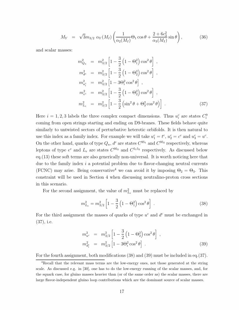
and scalar masses:

m2Qu

= m23/2

[

1 − 3

2

(

1 − Θ21

)

cos2 θ]

,

m2dc = m2

3/2

[

1 − 3

2

(

1 − Θ22

)

cos2 θ]

,

m2uc

i= m2

3/2

[

1 − 3Θ2i cos2 θ

]

,

m2ec = m2

3/2

[

1 − 3

2

(

1 − Θ22

)

cos2 θ]

,

m2Le

= m23/2

[

1 − 3

2

(

sin2 θ + Θ23 cos2 θ

)

]

. (37)

Here i = 1, 2, 3 labels the three complex compact dimensions. Thus uci are states C9

i

coming from open strings starting and ending on D9-branes. These fields behave quite

similarly to untwisted sectors of perturbative heterotic orbifolds. It is then natural to

use this index as a family index. For example we will take uc1 = tc, uc

2 = cc and uc3 = uc.

On the other hand, quarks of type Qu, dc are states C951 and C952 respectively, whereas

leptons of type ec and Le are states C952 and C5152 respectively. As discussed below

eq.(13) these soft terms are also generically non-universal. It is worth noticing here that

due to the family index i a potential problem due to flavor-changing neutral currents

(FCNC) may arise. Being conservative4 we can avoid it by imposing Θ2 = Θ3. This

constraint will be used in Section 4 when discussing neutralino-proton cross sections

in this scenario.

For the second assignment, the value of m2Le

must be replaced by

m2Le

= m23/2

[

1 − 3

2

(

1 − Θ21

)

cos2 θ]

. (38)

For the third assignment the masses of quarks of type uc and dc must be exchanged in

(37), i.e.

m2uc = m2

3/2

[

1 − 3

2

(

1 − Θ22

)

cos2 θ]

,

m2dc

i= m2

3/2

[

1 − 3Θ2i cos2 θ

]

. (39)

For the fourth assignment, both modifications (38) and (39) must be included in eq.(37).

4Recall that the relevant mass terms are the low-energy ones, not those generated at the string

scale. As discussed e.g. in [30], one has to do the low-energy running of the scalar masses, and, for

the squark case, for gluino masses heavier than (or of the same order as) the scalar masses, there are

large flavor-independent gluino loop contributions which are the dominant source of scalar masses.

17

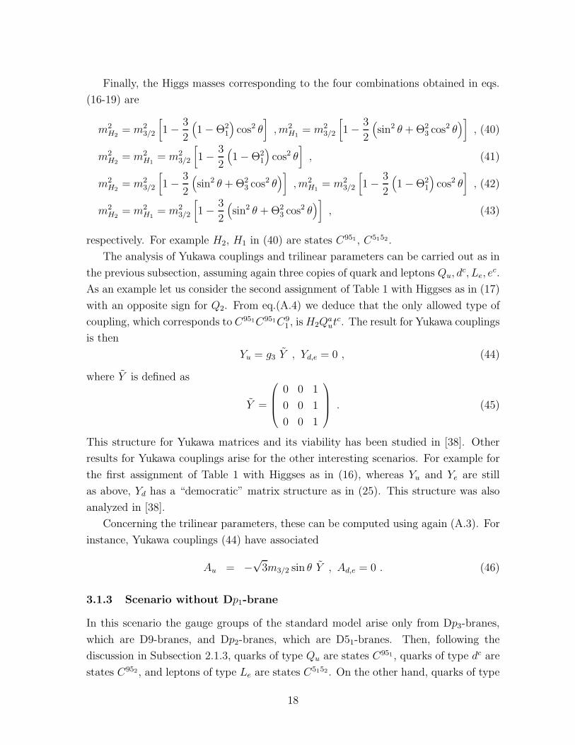
Finally, the Higgs masses corresponding to the four combinations obtained in eqs.

(16-19) are

m2H2

= m23/2

[

1 − 3

2

(

1 − Θ21

)

cos2 θ]

, m2H1

= m23/2

[

1 − 3

2

(

sin2 θ + Θ23 cos2 θ

)

]

, (40)

m2H2

= m2H1

= m23/2

[

1 − 3

2

(

1 − Θ21

)

cos2 θ]

, (41)

m2H2

= m23/2

[

1 − 3

2

(

sin2 θ + Θ23 cos2 θ

)

]

, m2H1

= m23/2

[

1 − 3

2

(

1 − Θ21

)

cos2 θ]

, (42)

m2H2

= m2H1

= m23/2

[

1 − 3

2

(

sin2 θ + Θ23 cos2 θ

)

]

, (43)

respectively. For example H2, H1 in (40) are states C951 , C5152 .

The analysis of Yukawa couplings and trilinear parameters can be carried out as in

the previous subsection, assuming again three copies of quark and leptons Qu, dc, Le, e

c.

As an example let us consider the second assignment of Table 1 with Higgses as in (17)

with an opposite sign for Q2. From eq.(A.4) we deduce that the only allowed type of

coupling, which corresponds to C951C951C91 , is H2Q

aut

c. The result for Yukawa couplings

is then

Yu = g3 Y , Yd,e = 0 , (44)

where Y is defined as

Y =

0 0 1

0 0 1

0 0 1

. (45)

This structure for Yukawa matrices and its viability has been studied in [38]. Other

results for Yukawa couplings arise for the other interesting scenarios. For example for

the first assignment of Table 1 with Higgses as in (16), whereas Yu and Ye are still

as above, Yd has a “democratic” matrix structure as in (25). This structure was also

analyzed in [38].

Concerning the trilinear parameters, these can be computed using again (A.3). For

instance, Yukawa couplings (44) have associated

Au = −√

3m3/2 sin θ Y , Ad,e = 0 . (46)

3.1.3 Scenario without Dp1-brane

In this scenario the gauge groups of the standard model arise only from Dp3-branes,

which are D9-branes, and Dp2-branes, which are D51-branes. Then, following the

discussion in Subsection 2.1.3, quarks of type Qu are states C951 , quarks of type dc are

states C952 , and leptons of type Le are states C5152 . On the other hand, quarks of type

18

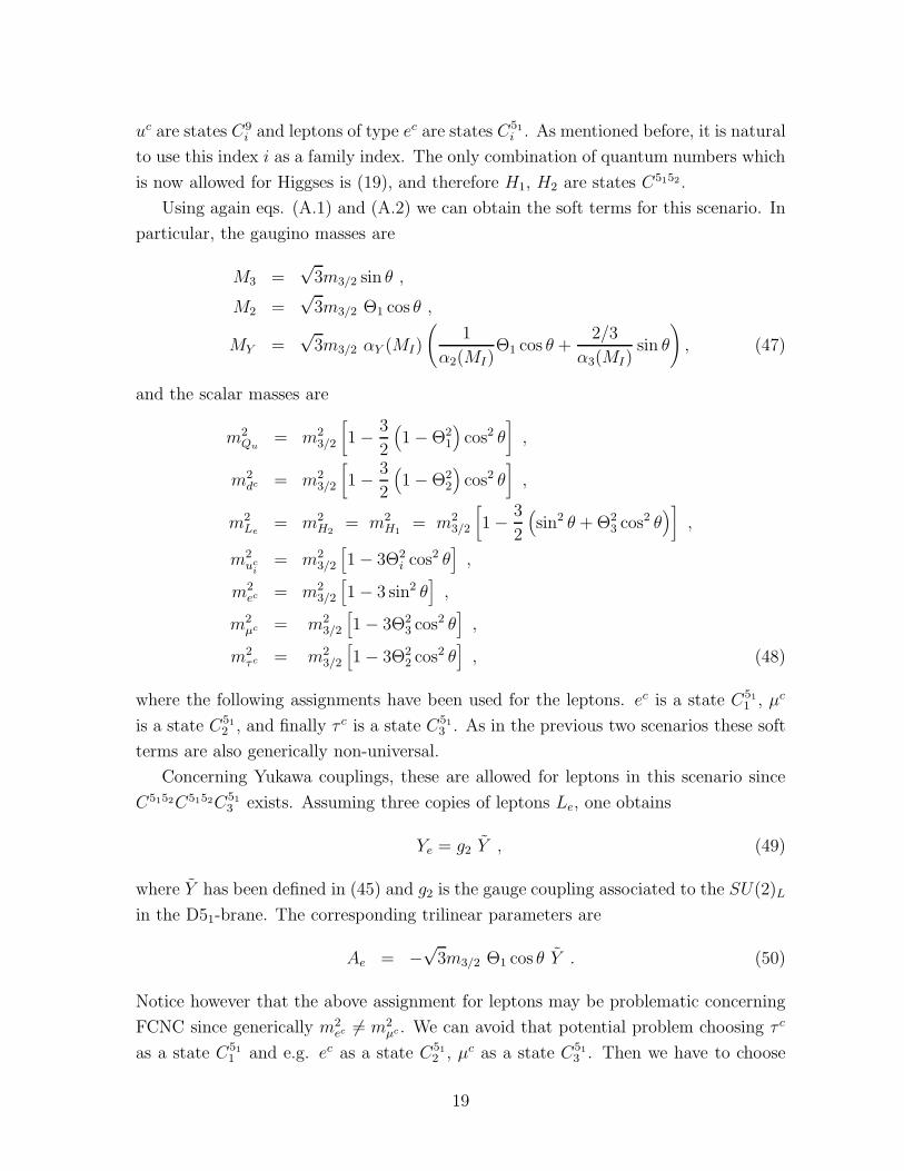
uc are states C9i and leptons of type ec are states C51

i . As mentioned before, it is natural

to use this index i as a family index. The only combination of quantum numbers which

is now allowed for Higgses is (19), and therefore H1, H2 are states C5152 .

Using again eqs. (A.1) and (A.2) we can obtain the soft terms for this scenario. In

particular, the gaugino masses are

M3 =√

3m3/2 sin θ ,

M2 =√

3m3/2 Θ1 cos θ ,

MY =√

3m3/2 αY (MI)

(

1

α2(MI)Θ1 cos θ +

2/3

α3(MI)sin θ

)

, (47)

and the scalar masses are

m2Qu

= m23/2

[

1 − 3

2

(

1 − Θ21

)

cos2 θ]

,

m2dc = m2

3/2

[

1 − 3

2

(

1 − Θ22

)

cos2 θ]

,

m2Le

= m2H2

= m2H1

= m23/2

[

1 − 3

2

(

sin2 θ + Θ23 cos2 θ

)

]

,

m2uc

i= m2

3/2

[

1 − 3Θ2i cos2 θ

]

,

m2ec = m2

3/2

[

1 − 3 sin2 θ]

,

m2µc = m2

3/2

[

1 − 3Θ23 cos2 θ

]

,

m2τc = m2

3/2

[

1 − 3Θ22 cos2 θ

]

, (48)

where the following assignments have been used for the leptons. ec is a state C51

1 , µc

is a state C51

2 , and finally τ c is a state C51

3 . As in the previous two scenarios these soft

terms are also generically non-universal.

Concerning Yukawa couplings, these are allowed for leptons in this scenario since

C5152C5152C51

3 exists. Assuming three copies of leptons Le, one obtains

Ye = g2 Y , (49)

where Y has been defined in (45) and g2 is the gauge coupling associated to the SU(2)L

in the D51-brane. The corresponding trilinear parameters are

Ae = −√

3m3/2 Θ1 cos θ Y . (50)

Notice however that the above assignment for leptons may be problematic concerning

FCNC since generically m2ec 6= m2

µc . We can avoid that potential problem choosing τ c

as a state C51

1 and e.g. ec as a state C51

2 , µc as a state C51

3 . Then we have to choose

19

uc1 = tc. Now, imposing Θ2 = Θ3, FCNC will not be present. This constraint will

be used in Section 4 when discussing neutralino-proton cross sections in this scenario.

Instead of the matrix structure (49) there will be a new matrix with the non-vanishing

entries in the second column.

On the other hand, Yukawa couplings for quarks of type u are vanishing since

couplings C5152C951C9i are forbidden. However, couplings C5152C951C952 are allowed

and therefore Yukawa couplings for quarks of type d exist. The matrix structure is like

in (25). In any case, as discussed for other scenarios in subsection 3.1.1, is difficult to

imagine how this scenario may give rise to the observed fermion mass hierarchies with

masses of quarks of type u arising from non-renormalizable terms.

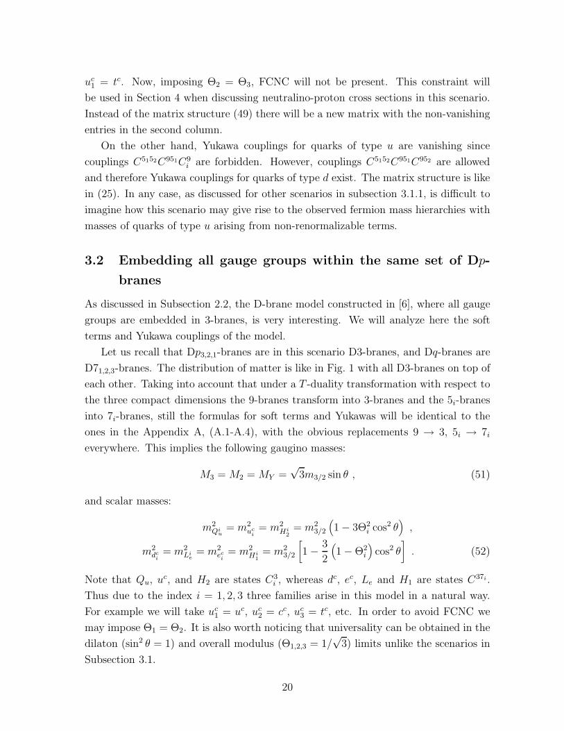
3.2 Embedding all gauge groups within the same set of Dp-

branes

As discussed in Subsection 2.2, the D-brane model constructed in [6], where all gauge

groups are embedded in 3-branes, is very interesting. We will analyze here the soft

terms and Yukawa couplings of the model.

Let us recall that Dp3,2,1-branes are in this scenario D3-branes, and Dq-branes are

D71,2,3-branes. The distribution of matter is like in Fig. 1 with all D3-branes on top of

each other. Taking into account that under a T -duality transformation with respect to

the three compact dimensions the 9-branes transform into 3-branes and the 5i-branes

into 7i-branes, still the formulas for soft terms and Yukawas will be identical to the

ones in the Appendix A, (A.1-A.4), with the obvious replacements 9 → 3, 5i → 7i

everywhere. This implies the following gaugino masses:

M3 = M2 = MY =√

3m3/2 sin θ , (51)

and scalar masses:

m2Qi

u= m2

uci= m2

Hi2

= m23/2

(

1 − 3Θ2i cos2 θ

)

,

m2dc

i= m2

Lie

= m2eci= m2

Hi1

= m23/2

[

1 − 3

2

(

1 − Θ2i

)

cos2 θ]

. (52)

Note that Qu, uc, and H2 are states C3i , whereas dc, ec, Le and H1 are states C37i .

Thus due to the index i = 1, 2, 3 three families arise in this model in a natural way.

For example we will take uc1 = uc, uc

2 = cc, uc3 = tc, etc. In order to avoid FCNC we

may impose Θ1 = Θ2. It is also worth noticing that universality can be obtained in the

dilaton (sin2 θ = 1) and overall modulus (Θ1,2,3 = 1/√

3) limits unlike the scenarios in

Subsection 3.1.

20

Let us now analyze the Yukawa couplings of the model [6]. Couplings of the type

C31C

32C

33 are allowed. Assuming that the physical Higgs H2 corresponds to C3

1 , the

following couplings exist: gH2Qctc and gH2Qtc

c, i.e.

Yu = g Y , (53)

where Y is defined as

Y =

0 0 0

0 0 1

0 1 0

. (54)

The corresponding trilinear parameters are

Au = −√

3m3/2 sin θ Y . (55)

Let us remark that in the presence of discrete torsion gH2Qttc may also be present [6].

On the other hand, couplings of the type C3i C

37iC37i are also allowed. Assuming that

the physical Higgs H1 corresponds to C373 , the coupling gQtbcH1 also exists, i.e.

Yb = g ¯Y , (56)

where ¯Y is defined as

¯Y =

0 0 0

0 0 0

0 0 1

. (57)

The trilinear parameters are

Ab = −√

3m3/2 sin θ ¯Y . (58)

More involved couplings with off-diagonal entries in the matrix for quarks of type d

are possible in some circumstances [6]. Finally, renormalizable Yukawa couplings for

leptons are not present since they are of the type C37C37C37 and these are not allowed.

4 Neutralino-nucleon cross sections in D-brane sce-

narios

Recently there has been some theoretical activity [43]-[49] analyzing the compatibility

of regions in the parameter space of the MSSM with the sensitivity of current (DAMA

[20], CDMS [21], HEIDELBERG-MOSCOW [22], HDMS prototype [23], UKDMC [24],

CANFRANC [25]) and projected (GENIUS [26], DAMA 250 kg. [20], CDMS Soudan

21

[21], etc.) dark matter detectors. In particular, DAMA and CDMS are sensitive to a

neutralino-nucleon cross section σχ0

1−p in the range of 10−6–10−5 pb. Working in the

supergravity framework for the MSSM with universal soft terms, it was pointed out in

[43, 44, 46, 49] that the large tanβ regime allows regions where the above mentioned

range of σχ0

1−p is reached. Besides, working with non-universal soft scalar masses mα,

σχ0

1−p ≈ 10−6 pb was also found for small values of tan β, if mα fulfil some special

conditions [43, 44, 46]. In particular, this was obtained for tanβ >∼ 25 (tan β >∼ 4)

working with universal (non-universal) soft terms in [46]. The case of non-universal

gaugino masses was also analyzed in [47] with interesting results.

The above analyses were performed assuming universality (and non-universality)

of the soft breaking terms at the unification scale, MGUT ≈ 1016 GeV, as it is usually

done in the MSSM literature. However, inspired by superstrings, where the unification

scale may be smaller, it was analyzed in [18] the sensitivity of the neutralino-nucleon

cross section to the value of the initial scale for the running of the soft breaking terms.

Working in the supergravity context with universal soft terms, the result was that

the smaller the scale is, the larger the cross section becomes. In particular, by taking

1010−12 GeV rather than 1016 GeV for the initial scale, the cross section increases

substantially σχ0

1−p ≈ 10−6–10−5 pb.

The natural extension of this analysis is to carry it out with explicit D-brane con-

structions. As mentioned in Subsection 3.1.2, the first attempts to study dark matter

within these constructions were carried out in [39]-[41] for the unification scale as the

initial scale and in [42] for an intermediate scale as the initial scale in the case of dila-

ton dominance. Here we will take into account the crucial issue of the D-brane origin

of the U(1)Y and its consequences on the matter distribution and soft terms in these

scenarios. Thus we will analyze the D-brane scenarios introduced in Section 2, using

their soft terms computed in Section 3. The fact that in these scenarios “intermediate”

initial scales and/or non-universal soft terms are possible allows us to think that large

cross sections, in the small tanβ regime, could be obtained in principle. Let us recall

that this can be understood from the variation in the value of µ, i.e. the Higgs mix-

ing parameter which appears in the superpotential W = µH1H2. Both, “intermediate”

scales and non-universality, can produce a decrease in the value of µ. When this occurs,

the Higgsino components, N13 and N14, of the lightest neutralino

χ01 = N11B

0 + N12W0 + N13H

01 + N14H

02 (59)

increase and therefore the scattering channels through Higgs exchange become impor-

tant. As a consequence the spin independent cross section also increases.

Before entering in details let us remark that we will work with the usual formulas

22

for the elastic scattering of relic LSPs on protons and neutrons that can be found in

the literature [19]. In particular, we will follow the re-evaluation of the rates carried

out in [45], using their central values for the hadronic matrix elements.

Let us discuss now the parameter space of our D-brane scenarios. As usual in

supersymmetric theories, the requirement of correct electroweak breaking leaves us

(modulo the sign of µ) with the following parameters. The soft breaking terms, scalar

and gaugino masses and trilinear parameters, and tanβ. Although formulas for the

soft terms obtained in Section 3 leave us in principle with five parameters, m3/2, θ and

Θi with i = 1, 2, 3, due to relation∑

i |Θi|2 = 1 only four of them are independent. In

our analysis we vary the parameters θ and Θi in the whole allowed range, 0 ≤ θ < 2π,

−1 ≤ Θi ≤ 1. For the gravitino mass we take m3/2 ≤ 300 GeV. Concerning Yukawa

couplings we will fix their values imposing the correct fermion mass spectrum at low

energies, i.e. we are assuming that Yukawa structures of D-brane scenarios give rise to

those values.

We will analyze first the scenario of Subsection 2.1.1 with three different sets of

Dp-branes, where the standard model gauge groups live. Since for the third and fourth

assignments of quantum numbers in Table 1 MI <∼ 3 × 108 GeV, and therefore m3/2

is too low to be phenomenologically interesting, we will consider only the soft masses

associated to the first and second assignments, i.e. the eight possible combinations

given by eqs. (12-14), (20-23). The discussion of the corresponding trilinear parameters

can be found below eq.(23).

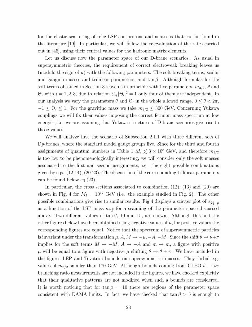
In particular, the cross sections associated to combination (12), (13) and (20) are

shown in Fig. 4 for MI = 1012 GeV (i.e. the example studied in Fig. 2). The other

possible combinations give rise to similar results. Fig 4 displays a scatter plot of σχ0

1−p

as a function of the LSP mass mχ0

1for a scanning of the parameter space discussed

above. Two different values of tan β, 10 and 15, are shown. Although this and the

other figures below have been obtained using negative values of µ, for positive values the

corresponding figures are equal. Notice that the spectrum of supersymmetric particles

is invariant under the transformation µ, A, M → −µ,−A,−M . Since the shift θ → θ+π

implies for the soft terms M → −M , A → −A and m → m, a figure with positive

µ will be equal to a figure with negative µ shifting θ → θ + π. We have included in

the figures LEP and Tevatron bounds on supersymmetric masses. They forbid e.g.

values of m3/2 smaller than 170 GeV. Although bounds coming from CLEO b → sγ

branching ratio measurements are not included in the figures, we have checked explicitly

that their qualitative patterns are not modified when such a bounds are considered.

It is worth noticing that for tan β = 10 there are regions of the parameter space

consistent with DAMA limits. In fact, we have checked that tan β > 5 is enough to

23

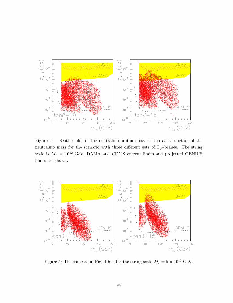
Figure 4: Scatter plot of the neutralino-proton cross section as a function of the

neutralino mass for the scenario with three different sets of Dp-branes. The string

scale is MI = 1012 GeV. DAMA and CDMS current limits and projected GENIUS

limits are shown.

Figure 5: The same as in Fig. 4 but for the string scale MI = 5 × 1015 GeV.

24

Figure 6: The same as in Fig. 4 but for the scenario with Dp1 = Dp3. The string scale

is MI = 8 × 109 GeV.

obtain compatibility with DAMA. Since the larger tanβ is, the larger the cross section

becomes, for tanβ = 15 these regions increase.

As discussed below eq.(6), larger values of the string scale may be obtained with

α1(MI) > 0.1. In particular we show the example where MI = 5 × 1015 GeV, cor-

responding to α1(MI) ≈ 1, in Fig. 5. Since the larger the scale is, the smaller the

cross section becomes, now the cross sections decrease with respect to the previous

case. In particular, tanβ > 10 is necessary in order to have compatibility with DAMA.

On the other hand, as discussed above, in the MSSM with universal soft terms at the

unification scale (which is close to the above MI), tanβ >∼ 20 was needed to obtain

compatibility. Clearly the non-universality of the soft terms in this string scenario

plays a crucial role increasing the cross sections.

Let us finally recall that both figures are obtained taking m3/2 ≤ 300 GeV, which

corresponds to squark masses mq <∼ 500 GeV at low energies. We have checked that

larger values of m3/2 produce cross sections below DAMA limits. In particular, the

right hand side and bottom of the figures will also be filled with points. Cross sections

below projected GENIUS limits will appear in both figures. On the other hand, it is

worth mentioning that the few isolated points in the plots with, in general, very large

values of the cross section correspond to values of the lightest stop mass extremely

close to the mass of the LSP, in particular (mt − mχ0

1

)/mt < 0.01.

25

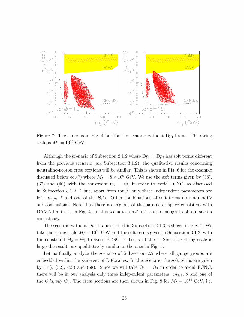
Figure 7: The same as in Fig. 4 but for the scenario without Dp1-brane. The string

scale is MI = 1016 GeV.

Although the scenario of Subsection 2.1.2 where Dp1 = Dp3 has soft terms different

from the previous scenario (see Subsection 3.1.2), the qualitative results concerning

neutralino-proton cross sections will be similar. This is shown in Fig. 6 for the example

discussed below eq.(7) where MI = 8× 109 GeV. We use the soft terms given by (36),

(37) and (40) with the constraint Θ2 = Θ3 in order to avoid FCNC, as discussed

in Subsection 3.1.2. Thus, apart from tan β, only three independent parameters are

left: m3/2, θ and one of the Θi’s. Other combinations of soft terms do not modify

our conclusions. Note that there are regions of the parameter space consistent with

DAMA limits, as in Fig. 4. In this scenario tan β > 5 is also enough to obtain such a

consistency.

The scenario without Dp1-brane studied in Subsection 2.1.3 is shown in Fig. 7. We

take the string scale MI = 1016 GeV and the soft terms given in Subsection 3.1.3, with

the constraint Θ2 = Θ3 to avoid FCNC as discussed there. Since the string scale is

large the results are qualitatively similar to the ones in Fig. 5.

Let us finally analyze the scenario of Subsection 2.2 where all gauge groups are

embedded within the same set of D3-branes. In this scenario the soft terms are given

by (51), (52), (55) and (58). Since we will take Θ1 = Θ2 in order to avoid FCNC,

there will be in our analysis only three independent parameters: m3/2, θ and one of

the Θi’s, say Θ3. The cross sections are then shown in Fig. 8 for MI = 1010 GeV, i.e.

26

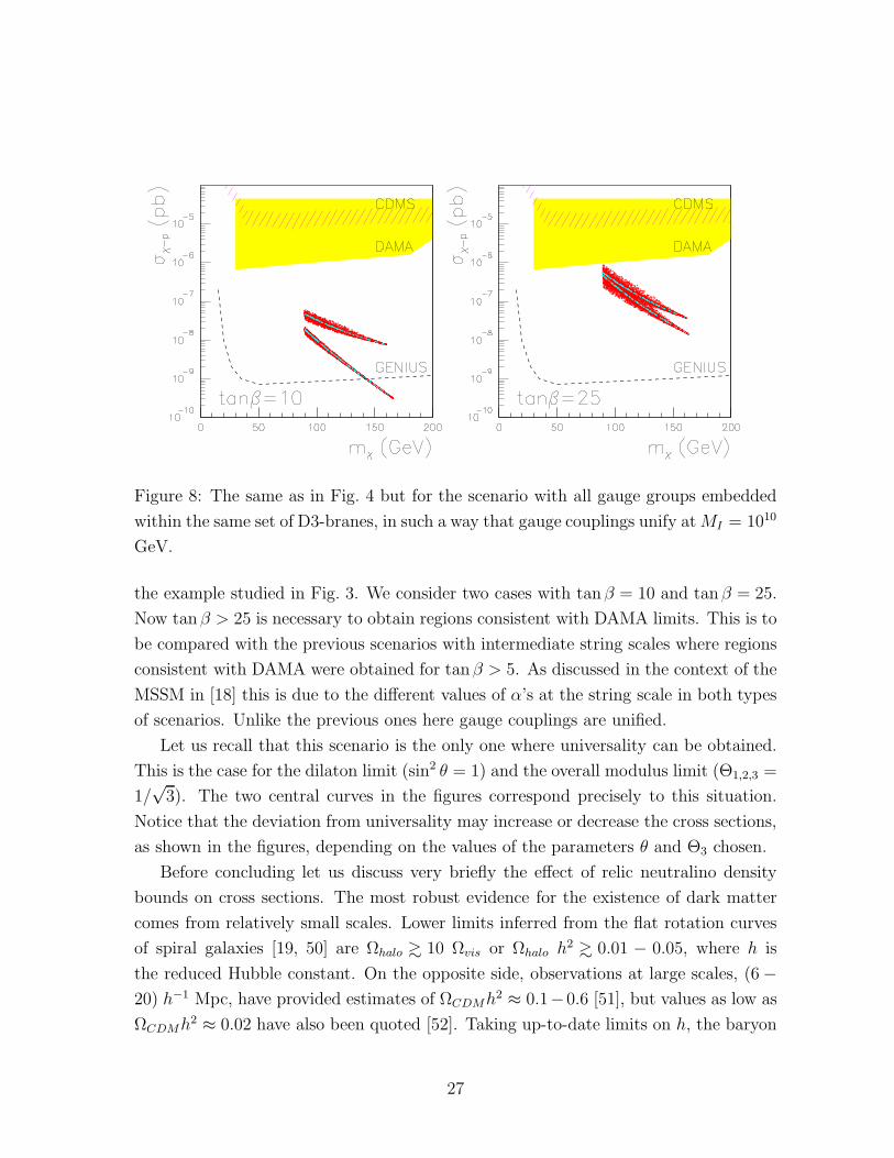
Figure 8: The same as in Fig. 4 but for the scenario with all gauge groups embedded

within the same set of D3-branes, in such a way that gauge couplings unify at MI = 1010

GeV.

the example studied in Fig. 3. We consider two cases with tanβ = 10 and tanβ = 25.

Now tanβ > 25 is necessary to obtain regions consistent with DAMA limits. This is to

be compared with the previous scenarios with intermediate string scales where regions

consistent with DAMA were obtained for tanβ > 5. As discussed in the context of the

MSSM in [18] this is due to the different values of α’s at the string scale in both types

of scenarios. Unlike the previous ones here gauge couplings are unified.

Let us recall that this scenario is the only one where universality can be obtained.

This is the case for the dilaton limit (sin2 θ = 1) and the overall modulus limit (Θ1,2,3 =

1/√

3). The two central curves in the figures correspond precisely to this situation.

Notice that the deviation from universality may increase or decrease the cross sections,

as shown in the figures, depending on the values of the parameters θ and Θ3 chosen.

Before concluding let us discuss very briefly the effect of relic neutralino density

bounds on cross sections. The most robust evidence for the existence of dark matter

comes from relatively small scales. Lower limits inferred from the flat rotation curves

of spiral galaxies [19, 50] are Ωhalo >∼ 10 Ωvis or Ωhalo h2 >∼ 0.01 − 0.05, where h is

the reduced Hubble constant. On the opposite side, observations at large scales, (6 −20) h−1 Mpc, have provided estimates of ΩCDMh2 ≈ 0.1−0.6 [51], but values as low as

ΩCDMh2 ≈ 0.02 have also been quoted [52]. Taking up-to-date limits on h, the baryon

27

density from nucleosynthesis and overall matter-balance analysis one is able to obtain

a favoured range, 0.01 <∼ ΩCDMh2 <∼ 0.3 (at ∼ 2σ CL) [53, 54]. Note that conservative

lower limits in the small and large scales are of the same order of magnitude.

In this work the expected neutralino cosmological relic density has been computed

according to well known techniques (see [19]). Although bounds coming from them

are not included in the above figures we have checked explicitly that their qualitative

patterns are not modified for most of the regions in figs. 4-7 when such a bounds

are considered. However the analysis of regions of the parameter space consistent

with DAMA limits is more delicate. From the general behaviour Ωχh2 ∝ 1/〈σann〉,where σann is the cross section for annihilation of neutralinos, it is expected that such

high neutralino-proton cross sections as those presented above will then correspond to

relatively low relic neutralino densities. We have seen that this is in fact the case. On

these grounds5, most of those points are at the border of the range of validity or below.

On the other hand, it is worth remarking that we are clearly below of the range of

validity for the whole regions in the scenario corresponding to Fig. 8.

5 Conclusions

In this paper we have analyzed different phenomenological aspects of D-brane scenarios.

First, assuming that the SU(3)c, SU(2)L and U(1)Y groups of the standard model come

from different sets of Dp-branes, intermediate values for the string scale MI ≈ 1010−12

GeV are obtained in a natural way. The reason is the following. Due to the D-brane

origin of the U(1)Y gauge group, the hypercharge is a linear combination of different

U(1) charges. Thus, in order to reproduce the low-energy data, i.e. the values of the

gauge couplings deduced from CERN e+e− collider LEP experiments, intermediate

values for MI are necessary. On the other hand, there is also the possibility that

the gauge groups of the standard model come from the same set of Dp-branes. In

fact explicit models with this property can be found in the literature. Again the

U(1)Y gauge group has a D-brane origin and therefore the normalization factor of the

hypercharge is not as the usual one in GUTs. The presence of additional doublets or

triplets allows to obtain intermediate values for the string scale.

Second, taking into account the matter assignment to the different Dp-branes of the

above scenarios, we have derived Yukawa couplings and soft supersymmetry-breaking

terms. The analysis of the soft terms has been carried out under the assumption

5Of course there is always the possibility that not all the dark matter in our Galaxy are neutralinos.

This would modify the analysis since e.g. Ωχ < ΩCDM .

28

of dilaton/moduli supersymmetry breaking, and they turn out to be generically non-

universal.

Finally, we have computed the neutralino-nucleon cross section of these D-brane

scenarios. This computation is extremely interesting since the lightest neutralino is a

natural candidate for dark matter in supersymmetric theories. Using the previously

obtained soft terms, and taking into account that the string scale MI is the initial

scale for their running, we have found regions in the parameter space of the D-brane

scenarios with cross sections in the range of 10−6–10−5 pb. For instance, this can be

obtained for tan β > 5. The above mentioned range is precisely the one where current

dark matter detectors, as e.g. DAMA and CDMS, are sensitive.

Acknowledgments

D.G. Cerdeno acknowledges the financial support of the Comunidad de Madrid through

a FPI grant. The work of S. Khalil was supported by PPARC. The work of C. Munoz

was supported in part by the Ministerio de Ciencia y Tecnologıa, and the European

Union under contract HPRN-CT-2000-00148. The work of E. Torrente-Lujan was

supported in part by the Ministerio de Ciencia y Tecnologıa.

A Appendix

We summarize in this Appendix the formulas for the soft terms [33] and Yukawa

couplings [35] in D-brane constructions, using one set of 9-branes and three sets of

5-branes, 5i. Assuming vanishing cosmological constant and neglecting phases, the

gaugino masses are given by

M9 =√

3m3/2 sin θ ,

M5i=

√3m3/2Θi cos θ , (A.1)

where M9 (M5i) are the masses of gauginos coming from open strings starting and

ending on 9 (5i)-branes. The scalar masses are given by

m2C9

i= m2

C5kj

= m23/2

(

1 − 3Θ2i cos2 θ

)

,

m2

C5ii

= m23/2

(

1 − 3 sin2 θ)

,

m2C95i = m2

3/2

[

1 − 3

2

(

1 − Θ2i

)

cos2 θ]

,

m2C5i5j = m2

3/2

[

1 − 3

2

(

sin2 θ + Θ2k cos2 θ

)

]

, (A.2)

29

where C9i denote matter fields coming from open strings starting and ending on 9-

branes (the index i which labels the three complex compact dimensions is very useful

in order to generate three families as we discuss in the text), C5i

i and C5i

j with i 6= j are

analogous to the previous ones but with 9-branes replaced by 5i-branes, C95i denote

matter fields coming from open strings starting (ending) on a 9-brane and ending

(starting) on a 5i-brane, C5i5j with i 6= j come from open strings starting in one type

of 5i brane and ending on a different type of 5j-brane. Finally the results for the

trilinear parameters are

AC9

1C9

2C9

3= AC9

iC95i C95i = −

√3m3/2 sin θ ,

AC

5i1

C5i2

C5i3

= AC

5ii

C95iC95i= A

C5ij

C5i5kC5i5k= −

√3m3/2Θi cos θ ,

AC5152C5351C5253 =

√3

2m3/2

[

sin θ −(

∑

i

Θi

)

cos θ

]

,

AC5i5j C95iC95j =

√3

2m3/2 [cos θ (Θk − Θi − Θj) − sin θ] , (A.3)

with i, j, k = 1, 2, 3 and i 6= j 6= k 6= i in the above equations. The angle θ and the

Θi with∑

i |Θi|2 = 1, just parameterize the direction of the goldstino in the S, Ti field

space.

On the other hand, the renormalizable Yukawa couplings which are allowed are

given by

LY = g9

(

C91C

92C

93 + C5152C5351C5253 +

3∑

i=1

C9i C95iC95i

)

+3∑

i,j,k=1

g5i

(

C5i

1 C5i

2 C5i

3

+ C5i

i C95iC95i + dijkC5i

j C5i5kC5i5k +1

2dijkC

5j5kC95j C95k

)

, (A.4)

with dijk = 1 if i 6= j 6= k 6= i, otherwise dijk = 0.

References

[1] B. Greene, K. Kirklin, P. Miron and G.G. Ross, Nucl. Phys. B278 (1986) 667,

B292 (1987) 602; J.A. Casas and C. Munoz, Phys. Lett. B209 (1988) 214, Phys.

Lett. B214 (1988) 63; J.A. Casas, E.K. Katehou and C. Munoz, Nucl. Phys. B317

(1989) 171; A. Font, L.E. Ibanez, H.P. Nilles and F. Quevedo, Phys. Lett. B210

(1988) 101; I. Antoniadis, J. Ellis, J. Hagelin and D. Nanopoulos, Phys. Lett. B231

(1989) 65.

[2] Z. Kakushadze, Phys. Lett. B434 (1998) 269; J. Lykken, E. Poppitz, S. Trivedi,

Nucl. Phys. B543 (1999) 105.

30

[3] G. Shiu and S.-H.H. Tye, Phys. Rev. D58 (1998) 106007.

[4] Z. Kakushadze and S.-H.H. Tye, Phys. Rev. D58 (1998) 126001.

[5] M. Cvetic, M. Plumacher, J. Wang, JHEP 0004 (2000) 004; G. Aldazabal, L.E.

Ibanez, F. Quevedo, hep-ph/0001083.

[6] G. Aldazabal, L.E. Ibanez, F. Quevedo and A.M. Uranga, JHEP 0008 (2000) 002.

[7] D. Bailin, G.V. Kraniotis and A. Love, hep-th/0011289.

[8] S.F. King and D.A.J. Rayner, hep-ph/0012076.

[9] J. Lykken, Phys. Rev. D54 (1996) 3693.

[10] N. Arkani-Hamed, S. Dimopoulos and G. Dvali, Phys. Rev. Lett. B249 (1998) 262;

I. Antoniadis, N. Arkani-Hamed, S. Dimopoulos and G. Dvali, Phys. Lett. B436

(1998) 263; I. Antoniadis and C. Bachas, Phys. Lett. B450 (1999) 83.

[11] K. Benakli, Phys. Rev. D60 (1999) 104002.

[12] C. Burgess, L.E. Ibanez and F. Quevedo, Phys. Lett. B447 (1999) 257.

[13] For a review, see e.g.: C. Munoz, hep-ph/9709329, and references therein.

[14] J.A. Casas, A. Lleyda and C. Munoz, Phys. Lett. B380 (1996) 59.

[15] J.A. Casas, A. Lleyda and C. Munoz, Phys. Lett. B389 (1996) 305.

[16] S.A. Abel, B.C. Allanach, F. Quevedo, L.E. Ibanez and M. Klein, JHEP 0012

(2000) 026.

[17] N. Kaloper and A. Linde, Phys. Rev. D59 (1999) 101303.

[18] E. Gabrielli, S. Khalil, C. Munoz and E. Torrente-Lujan, Phys. Rev. D63 (2001)

025008.

[19] For a review, see e.g.: G. Jungman, M. Kamionkowski and K. Griest, Phys. Rept.

267 (1996) 195, and references therein.

[20] R. Bernabei et al., Phys. Lett. B480 (2000) 23.

[21] R. Abusaidi et al., Phys. Rev. Lett. 84 (2000) 5699.

[22] Heidelberg-Moscow Collaboration, Phys. Rev. D59 (1998) 022001.

31

[23] Heidelberg-Moscow Collaboration, Phys. Rev. D63 (2001) 022001.

[24] P.F. Smith et al., Phys. Rep. 307 (1998) 275.

[25] Canfranc Underground Laboratory Collaboration, hep-ph/0011318.

[26] H.V. Klapdor-Kleingrothaus, L. Baudis, G. Heusser, B. Majorovits and H. Paes,

hep-ph/9910205.

[27] For a review, see: A. Brignole, L.E. Ibanez and C. Munoz, in the book ‘Per-

spectives on Supersymmetry’, Ed. G. Kane, (World Scientific, 1998) p. 125; hep-

ph/9707209.

[28] L.E. Ibanez and D. Lust, Nucl. Phys. B382 (1992) 305.

[29] V.S. Kaplunovsky and J. Louis, Phys. Lett. B306 (1993) 269.

[30] A. Brignole, L.E. Ibanez and C. Munoz, Nucl. Phys. B422 (1994) 125, B436 (1995)

747 (E); A. Brignole, L.E. Ibanez, C. Munoz and C. Scheich, Z. Phys. C74 (1997)

157.

[31] I. Antoniadis, E. Kiritsis and T.N. Tomaras, Phys. Lett. B486 (2000) 186.

[32] L.E. Ibanez, hep-ph/9804236.

[33] L.E. Ibanez, C. Munoz and S. Rigolin, Nucl. Phys. B553 (1999) 43.

[34] Particle Data Group, Eur. Phys. J. C15 (2000) 1.

[35] M. Berkooz and R.G. Leigh, Nucl. Phys. B483 (1997) 187.

[36] H. Fritzsch and D. Holtmannspotter, Phys. Lett. B338 (1994) 290; H. Fritzsch and

Z. Xing, Phys. Rev. D61 (2000) 073016.

[37] M. Brhlik, L. Everett, G.L. Kane and J. Lykken, Phys. Rev. D62 (2000) 035005; E.

Accomando, R. Arnowitt and B. Dutta, Phys. Rev. D61 (2000) 075010; T. Ibrahim

and P. Nath, Phys. Rev. D61 (2000) 093004; S. Khalil, T. Kobayashi and O. Vives,

Nucl. Phys. B580 (2000) 275; E. Gabrielli, S. Khalil and E. Torrente-Lujan, Nucl.

Phys. B594 (2001) 3; D. Carvalho, M. Gomez and S. Khalil, hep-ph/0101250.

[38] L. Everett, G.L. Kane and S.F. King, JHEP 0008 (2000) 012.

[39] S. Khalil, Phys. Lett. B484 (2000) 98.

32

[40] A. Corsetti and P. Nath, hep-ph/0003186.

[41] R. Arnowitt, B. Dutta and Y. Santoso, hep-ph/0005154.

[42] D. Bailin, G.V. Kraniotis and A. Love, Phys. Lett. B491 (2000) 161.

[43] A. Bottino, F. Donato, N. Fornengo and S. Scopel, Phys. Rev. D59 (1999) 095004.

[44] R. Arnowitt and P. Nath, Phys. Rev. D60 (1999) 044004.

[45] J. Ellis, A. Ferstl and K. Olive, Phys. Lett. B481 (2000) 304.

[46] E. Accomando, R. Arnowitt, B. Dutta and Y. Santoso, Nucl. Phys. B585 (2000)

124.

[47] A. Corsetti and P. Nath, hep-ph/0003186.

[48] J.L. Feng, K.T. Matchev and F. Wilczek, Phys. Lett. B482 (2000) 388.

[49] M.E. Gomez and J.D. Vergados, hep-ph/0012020.

[50] P. Salucci and M. Persic, astro-ph/9703027, astro-ph/9903432.

[51] see e.g.: W.L. Freedman, astro-ph/9905222, and references therein.

[52] N. Kaiser, astro-ph/9809341.

[53] B. Sadoulet, Rev. Mod. Phys. 71 (1999) 197.

[54] J.R. Primack, astro-ph/0007187; J.R. Primack and M.A.K. Gross, astro-

ph/0007165.

33