Imperial/TP/13/AH/04

KIAS-P14038

Mass-deformed Brane Tilings

Massimo Bianchi,a Stefano Cremonesi,b Amihay Hanany,b Jose Francisco

Morales,a Daniel Ricci Pacifici,c Rak-Kyeong Seongd

aDipartimento di Fisica, Universita di Roma “TorVergata” and I.N.F.N., Sezione di Roma

“TorVergata”, Via della Ricerca Scientifica, 00133 Roma, ItalybTheoretical Physics Group, The Blackett Laboratory, Imperial College London,

Prince Consort Road, London SW7 2AZ, United KingdomcDipartimento di Fisica e Astronomia, Universita degli Studi di Padova and I.N.F.N, Sezione

di Padova, Via Marzolo 8, 35131, Padova, ItalydSchool of Physics, Korea Institute for Advanced Study,

85 Hoegi-ro, Seoul 130-722, South Korea

E-mail: massimo.bianchi, morales@roma2.infn.it,

s.cremonesi, a.hanany@imperial.ac.uk,

daniel.riccipacifici@pd.infn.it, rkseong@kias.re.kr

Abstract: We study renormalization group flows among N = 1 SCFTs realized on

the worldvolume of D3-branes probing toric Calabi-Yau singularities, thus admitting

a brane tiling description. The flows are triggered by masses for adjoint or vector-like

pairs of bifundamentals and are generalizations of the Klebanov-Witten construction of

theN = 1 theory for the conifold starting from theN = 2 theory for the C2/Z2 orbifold.

In order to preserve the toric condition pairs of masses with opposite signs have to be

switched on. We offer a geometric interpretation of the flows as complex deformations

of the Calabi-Yau singularity preserving the toric condition. For orbifolds, we support

this interpretation by an explicit string amplitude computation of the gauge invariant

mass terms generated by imaginary self-dual 3-form fluxes in the twisted sector. In

agreement with the holographic a-theorem, the volume of the Sasaki-Einstein 5-base of

the Calabi-Yau cone always increases along the flow.

arX

iv:1

408.

1957

v1 [

hep-

th]

8 A

ug 2

014

Contents

1 Introduction 1

2 Brane tilings 4

2.1 Example: C2/Z3 × C 8

3 Mass deformations 9

3.1 C2/Z3 × C to SPP (L1,2,1) 10

3.2 Other flows 14

4 R-symmetry, a-maximization and volume minimization 19

4.1 Volume minimization 20

4.2 Volume ratios 23

5 Mass deformations as complex structure deformations

and Hilbert series 24

6 The string amplitude 27

6.1 The RR amplitude 30

7 Conclusions 31

A Details of the flows 32

A.1 C2/Zn × C to Lk,n−k,k 33

A.2 (C2/Zn × C)/Z2 to Lk,n−k,k/Z2 34

A.3 C3/Z2n to Lk,n−k,k/Z′2 35

A.4 PdP4b to PdP4a 36

1 Introduction

A large class of N = 1 superconformal gauge theories in four dimensions can be re-

alized on the worldvolume of a stack of D3-branes probing toric Calabi-Yau threefold

singularities in Type IIB string theory. The field content and interactions of such gauge

theories are elegantly described by a bipartite graph on the 2-torus, known as a dimer

– 1 –

model or brane tiling [1–3]. The faces, edges and nodes of the brane tiling are associ-

ated to U(N) gauge group factors, bifundamental/adjoint matter and superpotential

terms respectively.

A simple class of toric CY singularities consists of orbifolds of the form C3/Γ where

Γ is a finite Abelian subgroup of SU(3) [4–7]. For Abelian Γ, the brane tiling is made

of n = |Γ| hexagonal faces covering the torus. The superpotential, inherited from the

parent N = 4 theory, is cubic in this case and the global symmetry is at least U(1)3,

including the U(1)R R-symmetry of the N = 1 superconformal theory.

When one of the complex planes is invariant under Γ, the singularity is actually of

the form C2/Zn × C and supersymmetry is enhanced to N = 2. These theories admit

mass deformations which break N = 2 supersymmetry down to N = 1. Integrating

out the massive fields, the theory flows to an N = 1 superconformal fixed-point in

the IR with a quartic – in general non-toric – super-potential. As shown by Klebanov

and Witten [8], the conifold singularity can be obtained in this way, by perturbing the

quiver gauge theory on the worldvolume of D3-branes probing the C2/Z2 × C orbifold

singularity with mass terms for the adjoint fields. Toricity is preserved when the two

mass parameters are equal and opposite. The brane tiling of the conifold theory is

made of two square faces covering the torus like a chessboard [2].

This construction admits a natural generalization to RG flows triggered by mass

deformations of N = 2 superconformal theories for D3 branes probing C2/Zn × C[9]. The generalization starts with a quiver gauge theory with n adjoint fields – one

for each U(N) factor – besides the bifundamental matter. By giving masses to any

of the adjoint fields, one generates a flow to a new – in general non-toric – N = 1

superconformal gauge theory. As we will review, toricity can be preserved by choosing

the mass parameters to be all equal with alternating signs in a sequence of k pairs

of adjoints. In addition, a field redefinition is required in the IR to restore the toric

property of the superpotential. The resulting quiver gauge theory is associated to the

toric singularity C(Lk,n−k,k), where C(X) denotes the cone over X, also known as a

generalized conifold.1 Pictorially, the flow may be thought of as the result of squeezing

2k strips of hexagonal faces in the brane tiling down to 2k strips of squares. The case

C2/Z3 ×C leading to the suspended pinch point (SPP) singularity [14] – also denoted

by L1,2,1 – is an example which we consider in this work.

The Type IIA dual description of these models a la Hanany-Witten, i.e. in terms of

D4-branes wrapping a circle and suspended in between n NS5-branes [15–17], suggests

that mass deformations can be interpreted as complex deformations of the singularity.

1To simplify the notation, we drop C(...) in naming Calabi-Yau cones and their corresponding

brane tilings in the rest of this work. Lk,n−k,k are members of a larger class of toric Sasaki-Einstein

5-fold called La,b,c [10], whose dual quiver gauge theories were found in [11–13].

– 2 –

Indeed, when the n NS5-branes are parallel to one another in the directions transverse

to the D4-branes, the configuration enjoys N = 2 supersymmetry. The adjoint chiral

multiplet inside the N = 2 vector multiplet corresponds to moving the D4-branes along

the NS5 brane or turning a Wilson line along the circle wrapped by the D4-branes. If

the NS5-branes are rotated by generic angles, supersymmetry is completely broken.

N = 1 supersymmetry is restored whenever the NS5-branes wrap complex planes in

C3. The masses of the adjoints are the complexified relative angles between NS5-branes.

The flow described above corresponds to the case where k out of the n NS5 branes are

rotated.

In the IIB description in terms of D3-branes on C2/Zn × C, the mass terms can

be realized as imaginary self-dual fluxes of type (2,1) as required by supersymmetry.

Fluxes of this type arise from the twisted sector and are associated to 3-forms ω(1,1)∧dZwith ω(1,1) being one of the twisted (1,1)-forms dual to an exceptional 2-cycle of the

ALE hyperkahler singularity C2/Zn and dZ being the holomorphic one-form on C.

Since one leg is non-compact, the flux is not quantized. While untwisted fluxes do

not discriminate among the various nodes of the quiver, or the various faces of the

brane tiling, twisted fluxes instead allow for different masses for the various fields as

required for the RG flow. Moreover, the counting of twisted sectors, n− 1 in this case,

precisely matches the counting of independent mass deformations or the counting of

relative rotations in the NS5-brane picture. Further evidence for this correspondence

is obtained by computing the string disk amplitude involving the insertions of a 3-form

field strength from the closed string twisted sector and two open string fermions.

Our construction is not limited to flows starting from N = 2 orbifold quivers, but

it applies to more general mass flows connecting two N = 1 superconformal theories.

We consider cases where the starting theory is or is not of orbifold type. The flows in

both cases are triggered by mass terms for bifundamental matter. As for deformations

of N = 2 theories, we show that in order to restore toricity in the IR after integrating

out the massive matter, one has to switch on equal mass parameters opposite in pairs,

each giving mass to two chiral super-fields. We illustrate this construction for the flows

(C2/Zn×C)/Z2 → Lk,n−k,k/Z2, C3/Z2n → Lk,n−k,k/Z′2 and PdP4b → PdP4a.2 A crucial

role in these RG flows is played by accidental symmetries which appear after integrating

out the massive fields and which restore the toric U(1)3 symmetry in the IR.

The plan of the paper is as follows. In section §2, we review brane tilings and

present the brane tiling for C2/Z3 × C as an example. Section §3 then discusses

mass deformations of brane tilings. The focus is on the RG flow C2/Z3 × C → L1,2,1

2Arising from D3-branes probing a non-compact CY 3-fold which is a complex cone over a toric

(pseudo) del Pezzo surface PdP4.

– 3 –

and then on the generalizations to other RG flows: (C2/Zn × C)/Z2 → Lk,n−k,k/Z2,

C3/Z2n → Lk,n−k,k/Z′2 and PdP4b → PdP4a. Section §4 then discusses a-maximization

and volume minimization in order to identify the superconformal R-symmetry at the

IR fixed point and to check that central charges decrease along the RG flows in accor-

dance with the a-theorem. Section §5 discusses the complex structure deformations of

the Calabi-Yau cones under mass deformations and the relation between Hilbert series

of the toric Calabi-Yau cones associated to the UV and the IR theories. Section §6 out-

lines with an explicit computation of the disk amplitudes the correspondence between

mass deformations in the boundary SCFT and the effect of 3-form fluxes in the bulk.

The paper closes with concluding remarks in section §7. The appendix contains details

of the RG flows induced by mass deformations; this includes the UV superpotential,

the mass terms, the IR superpotential, and the field redefinitions, if any, which are

needed to restore toricity.

2 Brane tilings

In this section we review brane tilings, which encode the data defining superconformal

quiver gauge theories on the worldvolume of D3-branes at toric Calabi-Yau cone singu-

larities. Brane tilings lead to a powerful forward algorithm [2, 3, 18–20] for computing

the vacuum moduli spaces of superconformal quiver gauge theories.

Brane tiling dictionary. A brane tiling is a bipartite graph on a 2-torus, i.e. a

covering of the 2-torus by even-sided polygonal faces bounded by edges connecting a

black to a white node. The black or white coloring of nodes corresponding to the

bipartiteness of the graph determines an orientation around vertices, which we take

by convention to be clockwise around white nodes and counter-clockwise around black

nodes. This in turn induces an orientation of the dual graph, the periodic quiver

diagram of the gauge theory.

The brane tiling/gauge theory dictionary is as follows:

• Faces are associated to U(N)i gauge group factors. We use F for the total

number of faces.

• Edges adjacent to faces i and j represent chiral superfields Xi j transforming in

the bifundamental representation of the associated gauge groups U(N)i×U(N)j.

The quiver orientation of the bifundamental field Xi j is given by the orientation

– 4 –

around the black and white nodes at the two ends of the corresponding tiling

edge. We denote by E the total number of edges.

• White (black) nodes correspond to positive (negative) monomial terms in the

superpotential W made of the products of the bifundamental fields associated to

the edges which end on the node and which are ordered in a clockwise (counter-

clockwise) fashion. The bipartite nature of the graph implies that every field

appears in the superpotential precisely once in a positive and once in a negative

term. We call this property the toric condition [18]. We denote by V the total

number of vertices.

The incidence matrix dG×E incorporates the charges of the chiral fields under the

U(1)i factor of the U(N)i = U(1)i × SU(N)i gauge groups. G is the number of gauge

groups, which equals the number of faces F of the tiling. In this work, we will concen-

trate on the Abelian case with N = 1, such that the incidence matrix fully incorporates

the gauge charges of the theory. The ith-entry is −1 for Xi j, +1 for Xj i and zero oth-

erwise. The matrix dG×E has G− 1 linearly independent rows that can be collected in

a separate matrix ∆G−1×E.

The Kasteleyn matrix K is a matrix which encodes information about the con-

nectivity of the bipartite diagram. Rows and columns index black nodes bm and white

wn nodes respectively and the entries of the matrix are associated to edges. An edge

X(m,n) between nodes (bm, wn) has a winding number (ha, hb) associated to the a, b-

cycles and the boundaries of the fundamental domain of the 2-torus. Accordingly,

elements of the Kasteleyn matrix take the following form,

Kmn(z1, z2) =∑

X(m,n)

zha(X(m,n))1 z

hb(X(m,n))2 , (2.1)

where z1, z2 are the fugacities for the winding numbers along the a- and b-cycles of the

2-torus respectively.

The permanent of the Kasteleyn matrix, also known as the characteristic polyno-

mial of the brane tiling,

perm K(z1, z2) =∑ni

cn1,n2zn11 zn2

2 (2.2)

encodes the toric diagram of the singularity. More precisely, the absolute values of the

coefficients |cn1,n2| give the multiplicities of the points (n1, n2) in the toric diagram.

– 5 –

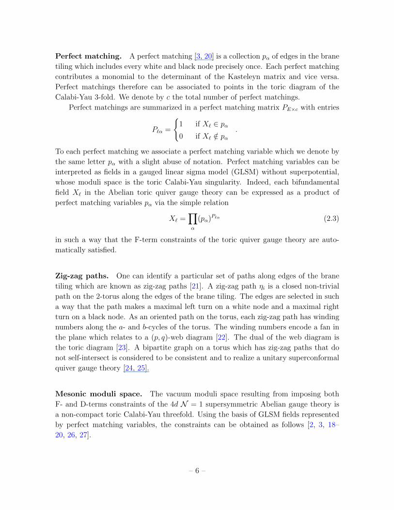
Perfect matching. A perfect matching [3, 20] is a collection pα of edges in the brane

tiling which includes every white and black node precisely once. Each perfect matching

contributes a monomial to the determinant of the Kasteleyn matrix and vice versa.

Perfect matchings therefore can be associated to points in the toric diagram of the

Calabi-Yau 3-fold. We denote by c the total number of perfect matchings.

Perfect matchings are summarized in a perfect matching matrix PE×c with entries

P`α =

1 if X` ∈ pα0 if X` /∈ pα

.

To each perfect matching we associate a perfect matching variable which we denote by

the same letter pα with a slight abuse of notation. Perfect matching variables can be

interpreted as fields in a gauged linear sigma model (GLSM) without superpotential,

whose moduli space is the toric Calabi-Yau singularity. Indeed, each bifundamental

field X` in the Abelian toric quiver gauge theory can be expressed as a product of

perfect matching variables pα via the simple relation

X` =∏α

(pα)P`α (2.3)

in such a way that the F-term constraints of the toric quiver gauge theory are auto-

matically satisfied.

Zig-zag paths. One can identify a particular set of paths along edges of the brane

tiling which are known as zig-zag paths [21]. A zig-zag path ηi is a closed non-trivial

path on the 2-torus along the edges of the brane tiling. The edges are selected in such

a way that the path makes a maximal left turn on a white node and a maximal right

turn on a black node. As an oriented path on the torus, each zig-zag path has winding

numbers along the a- and b-cycles of the torus. The winding numbers encode a fan in

the plane which relates to a (p, q)-web diagram [22]. The dual of the web diagram is

the toric diagram [23]. A bipartite graph on a torus which has zig-zag paths that do

not self-intersect is considered to be consistent and to realize a unitary superconformal

quiver gauge theory [24, 25].

Mesonic moduli space. The vacuum moduli space resulting from imposing both

F- and D-terms constraints of the 4d N = 1 supersymmetric Abelian gauge theory is

a non-compact toric Calabi-Yau threefold. Using the basis of GLSM fields represented

by perfect matching variables, the constraints can be obtained as follows [2, 3, 18–

20, 26, 27].

– 6 –

• The F-terms ∂XW = 0 are solved thanks to the introduction of perfect matching

variables, which are defined modulo an Abelian gauge symmetry which leaves

(2.3) invariant. The charges of the perfect matching variables under this gauge

symmetry are encoded in the charge matrix

QF (c−G−2)×c = ker (PE×c) , (2.4)

• The D-term charge matrix QD (G−1)×c is defined by the relation

∆(G−1)×e = QD (G−1)×c·P tc×e . (2.5)

where ∆(G−1)×e is the matrix formed by the G− 1 independent rows of dG×e.3

• One can combine the F - and D- charges into the total charge matrix of the GLSM,

Qt (c−3)×c =

(QF

QD

). (2.6)

The mesonic moduli space of the Abelian toric quiver gauge theory can be expressed

as a Kahler quotient of the ring of perfect matching variables Cc by the U(1)c−3-action

Qt,

Mmes = Cc//Qt . (2.7)

The integer kernel of Qt,

Gt = ker(Qt) , (2.8)

is a matrix whose rows are the coordinates of the points in the toric diagram associated

to the c perfect matchings.

The Hilbert series. The Hilbert series is a generating function which counts chiral

gauge invariant operators. The Hilbert series of the mesonic moduli space (2.8) counts

the number of U(1)c−3-invariant monomials made out of the c perfect matching variables

pα. It is computed using the Molien integral

g(tα;Mmes) =c−3∏i=1

∮|zi|=1

dzi2πizi

c∏α=1

1

1− tα∏c−3

j=1 z(Qt)jαj

, (2.9)

3The number of incoming and outgoing arrows at each quiver node is the same, ensuring gauge

anomaly cancellation. This results in ∆(G−1)×e which forms the G− 1 independent rows of the quiver

incidence matrix dG×e.

– 7 –

where tα is the fugacity corresponding to the perfect matching variable pα.

The Hilbert series encodes information about the generators of the moduli space

as well as the relations formed amongst them. This information can be extracted from

the so called plethystic logarithm [28, 29] of the Hilbert series g1(yα) defined as

PL[g(tα;Mmes)] =∞∑k=1

µ(k)

klog[g(tkα)

]=∑i

niMi(tα) (2.10)

where µ is the Mobius function, Mi(tα) are monomials made of fugacities tα and niare integers. The Hilbert series can be reconstructed from its plethystic logarithm and

written in the simple product form

g(tα;Mmes) =∏i

1

(1−Mi)ni= PE

[∑i

niMi

], (2.11)

where PE refers to the plethystic exponential.4 In particular, when PL[g(tα;Mmes)]

contains a finite number of terms, the spaceMmes is said to be a complete intersection.5

It is parametrized by the generators corresponding to the monomials Mi(tα);ni > 0satisfying a finite number of relations corresponding to the monomials Mi(tα);ni < 0.

Simple representatives in the class of complete intersections are Abelian orbifolds

of the form C2/Zn × C with the Hilbert series [28]

g(tα;C2/Zn × C) =1

n

n∑h=1

1∏3α=1(1− ωaαhn tα)

=(1− tn1 tn2 )

(1− tn1 )(1− tn2 )(1− t1t2)(1− t3)

(2.12)

with ωn = e2πin and aα = (1,−1, 0). The result in the right hand side shows that the

orbifold can be viewed as a hypersurface xy = wn in C4 with coordinates (x, y, w, z).

2.1 Example: C2/Z3 × C

Let us illustrate the brane tiling tools in the simple case of C2/Z3×C. The associated

quiver, brane tiling and toric diagrams are displayed in Figure 1.

The tiling is made of hexagons (as is always the case for orbifolds of C3) with

F = 3 faces associated to three U(1) nodes in the quiver diagram and E = 9 edges

4The plethystic exponential of a multivariate function f(t1, ..., tn) that vanishes at the origin,

f(0, ..., 0) = 0, is defined as PE [f(t1, t2, . . . , tn)] = exp(∑∞

k=11kf(tk1 , · · · , tkn)

). Its inverse is the

plethystic logarithm PL.5When a complete intersection has only one relation, the corresponding space is called a hypersur-

face.

– 8 –

3 2

1 1

1

13

2 3

2 3 1

2 3 1

2 3 1 2

2 3 1 2

1 2 3

3

3

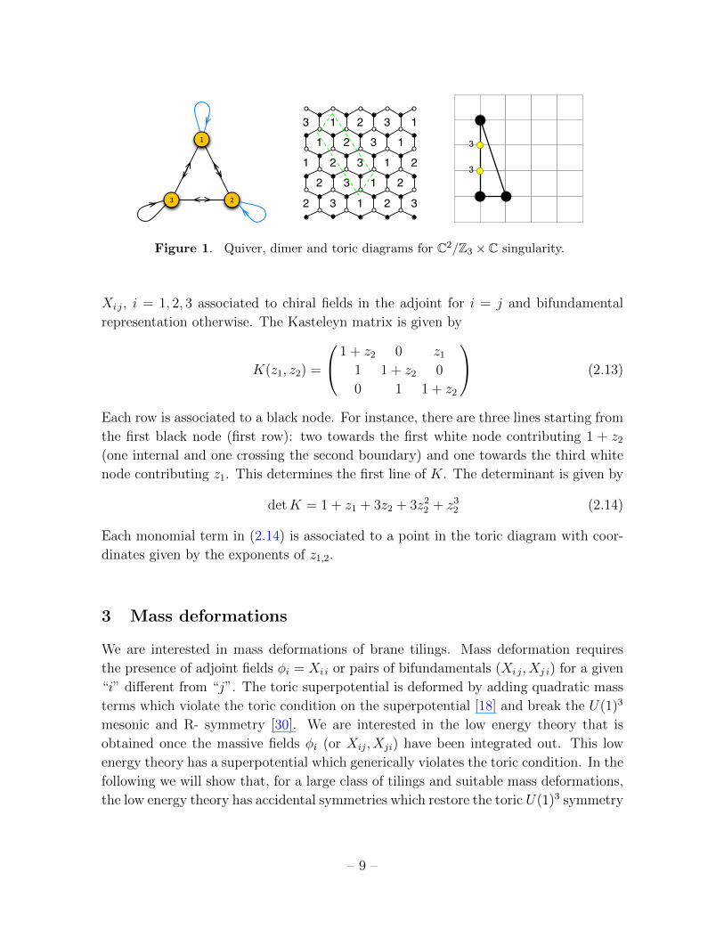
Figure 1. Quiver, dimer and toric diagrams for C2/Z3 × C singularity.

Xi j, i = 1, 2, 3 associated to chiral fields in the adjoint for i = j and bifundamental

representation otherwise. The Kasteleyn matrix is given by

K(z1, z2) =

1 + z2 0 z1

1 1 + z2 0

0 1 1 + z2

(2.13)

Each row is associated to a black node. For instance, there are three lines starting from

the first black node (first row): two towards the first white node contributing 1 + z2

(one internal and one crossing the second boundary) and one towards the third white

node contributing z1. This determines the first line of K. The determinant is given by

detK = 1 + z1 + 3z2 + 3z22 + z3

2 (2.14)

Each monomial term in (2.14) is associated to a point in the toric diagram with coor-

dinates given by the exponents of z1,2.

3 Mass deformations

We are interested in mass deformations of brane tilings. Mass deformation requires

the presence of adjoint fields φi = Xi i or pairs of bifundamentals (Xi j, Xj i) for a given

“i” different from “j”. The toric superpotential is deformed by adding quadratic mass

terms which violate the toric condition on the superpotential [18] and break the U(1)3

mesonic and R- symmetry [30]. We are interested in the low energy theory that is

obtained once the massive fields φi (or Xij, Xji) have been integrated out. This low

energy theory has a superpotential which generically violates the toric condition. In the

following we will show that, for a large class of tilings and suitable mass deformations,

the low energy theory has accidental symmetries which restore the toric U(1)3 symmetry

– 9 –

group. The accidental symmetry is made manifest by certain field redefinitions of the

massless fields which restore the toric condition for the superpotential.

We focus on brane tilings which have at least two adjacent strips of hexagonal faces

and consider the effect of give mass to the hypermultiplets along these strips. A strip

made of a single type of faces leads to adjoint edges while two alternating faces along the

strip leads to bifundamental matter. We collectively label the massive fields X(m) and

the light fields X(l) to highlight their different roles. We consider the mass-deformed

superpotential

Wdeformed(X(m), X(l)) = W (X(m), X(l)) + ∆W (X(m)) (3.1)

where W (X(m), X(l)) is the initial toric superpotential and ∆W (X(m)) is deformation

of one of the following types

• Adjoint: ∆W = m2

(φ2i1− φ2

i2) or

• Bifundamental: ∆W = m(Xi1j1Xj1i1 −Xi2j2Xj2i2),

possibly involving several pairs of mass terms, all with the same mass parameter m.

Integrating out the massive fields X(m), by solving their F-term equations

∂

∂X(m)Wdeformed(X(m), X(l)) = 0 (3.2)

in terms of the light components X(l), one finds a non-toric superpotential Wlow(X(l))

for the light fields. We are able to restore the toric condition by field redefinitions of

the light fields

X ′i j = Xi j +1

m

∑k

c(ij)k Xi kXk j or φ′i = φi +

1

m

∑k

c(ij)k Xi kXk j (3.3)

with some judicious choice of the coefficients c(ij)k . The low energy superpotential

Wlow(X(l)), rewritten in terms of the new variables X(l)′ can be shown to satisfy the

toric condition. As such the IR fixed point of the RG flow is associated to a new brane

tiling. In the following sections we consider some simple examples of mass-deformed

brane tilings.

3.1 C2/Z3 × C to SPP (L1,2,1)

We first illustrate mass deformation of brane tilings in our working example of C2/Z3×C. The starting super-potential is

W = φ1 (X13X31 −X12X21) + φ2 (X21X12 −X23X32) + φ3 (X32X23 −X31X13) (3.4)

– 10 –

3

3

3

1 2

1 2 3

1 2 3

1 2 3

1 2 3

3

3

3

3

2

1 2 3

1 2 3

1 2 3

1 2 3

3

3

3

3

2

1 2 3

1 2 3

1 2 3

1 2 3

3

Figure 2. Flow from C2/Z3 × C to L1,2,1.

3

3 2

Figure 3. Toric diagrams for the C2/Z3 × C case (on the left) and for SPP (on the right)

before and after the mass deformation. Mass deformation amounts to a displacement of an

extremal toric point.

The corresponding brane tiling and quiver diagram are shown in Figure 1. We consider

the mass deformation

∆W =m

2

(φ2

1 − φ22

). (3.5)

In the Type IIA description, this corresponds to rotating the NS5-brane between D4-

branes 1 and 2.

Along the flow, massive fields can be integrated out. The effective superpotential

at the infrared end of the flow is found by solving the mass-deformed F-term conditions

for φ1 and φ2 in favor of the light components

φ1 =1

m(X12X21 −X13X31) , φ2 =

1

m(X21X12 −X23X32) . (3.6)

Substituting this into the deformed superpotential Wdeformed = W + ∆W one finds a

non-toric superpotential. Remarkably, a toric superpotential is recovered under the

– 11 –

1 2 3

4

5

1 2 3

4

5

1

2

3

4

5

Figure 4. Mass deformation for the brane tiling of C2/Z3×C with zig-zag paths. η2 inverts

its direction during the mass deformation while the adjacency of the zig-zag paths is preserved.

field redefinitions

φ3 = φ′3 −1

2m(X31X13 +X32X23)

X12X21 = mX ′12X′21 , (3.7)

Indeed, by plugging (3.6) and (3.7) into Wdeformed, one finds the superpotential

Wfinal = φ3 (X32X23 −X31X13) +X ′12X′21X13X31 −X ′21X

′12X23X32 . (3.8)

The field content and the superpotential in (3.8) are those of the suspended pinch point

theory [18, 27, 31], also known as the theory for L1,2,1.

Interestingly, the result of integrating out the massive fields and shifting the light

fields can be visualized in the brane tiling as squeezing two consecutive strips of hexago-

nal faces into two strips of square faces as illustrated in Figure 2. The left side of Figure

2 shows the brane tiling for C2/Z3 × C. Edges associated to massive fields are drawn

in blue. These fields are aligned along a deformation strip made of two neighboring

arrays of hexagonal faces. The remaining internal edges in the deformation strip are

drawn in red and form a closed cycle on the 2-torus which we call the deformation line.

In order to obtain the brane tiling of the low energy theory, we need to remove the blue

– 12 –

1 2 3

4

5

1

2

3

4

5

3

3 2

1

2

3 4

5

1

3

4

2

5

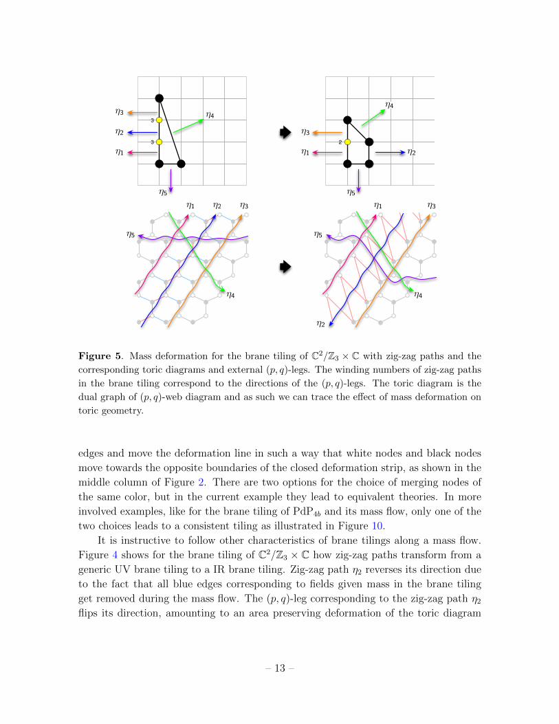
Figure 5. Mass deformation for the brane tiling of C2/Z3 × C with zig-zag paths and the

corresponding toric diagrams and external (p, q)-legs. The winding numbers of zig-zag paths

in the brane tiling correspond to the directions of the (p, q)-legs. The toric diagram is the

dual graph of (p, q)-web diagram and as such we can trace the effect of mass deformation on

toric geometry.

edges and move the deformation line in such a way that white nodes and black nodes

move towards the opposite boundaries of the closed deformation strip, as shown in the

middle column of Figure 2. There are two options for the choice of merging nodes of

the same color, but in the current example they lead to equivalent theories. In more

involved examples, like for the brane tiling of PdP4b and its mass flow, only one of the

two choices leads to a consistent tiling as illustrated in Figure 10.

It is instructive to follow other characteristics of brane tilings along a mass flow.

Figure 4 shows for the brane tiling of C2/Z3 × C how zig-zag paths transform from a

generic UV brane tiling to a IR brane tiling. Zig-zag path η2 reverses its direction due

to the fact that all blue edges corresponding to fields given mass in the brane tiling

get removed during the mass flow. The (p, q)-leg corresponding to the zig-zag path η2

flips its direction, amounting to an area preserving deformation of the toric diagram

– 13 –

as shown in Figure 5. In fact, the new toric diagram is obtained from the old one by

moving a single extremal toric point as illustrated in Figure 3. A few other zig-zag

paths change their directions as well, but do not completely reverse their direction.

This is governed by an overall (p, q)-charge conservation of zig-zag paths in the brane

tiling.

In general, we observe for all examples presented in this work that mass flow of

a brane tiling amounts to the displacement of toric points in the corresponding toric

diagram and the reversal of (p, q)-leg directions in the corresponding dual (p, q)-web

diagram. Furthermore, we remark that the area and hence the number of lattice points

along the perimeter of the toric diagram of the UV and IR toric Calabi-Yau geometries

are invariant because the mass deformation does not alter the number of anomalous

and non-anomalous baryonic symmetries.6

3.2 Other flows

The analysis in the last section can be applied mutatis mutandis to a large class of

brane tilings admitting mass deformations. In Figure 6, we list three infinite sequences

of flows starting from Abelian orbifolds of C3.

• C2/Zn×C→ Lk,n−k,k: These flows are generated by giving identical masses to k

pairs of adjoint chiral multiplets which belong to N = 2 vector multiplets.

• (C2/Zn × C)/Z2 → Lk,n−k,k/Z2: These flows are generated by giving identical

masses to 2k pairs of chiral multiplets in bifundamental representations.

• C3/Z2n → Lk,n−k,k/Z′2: These singularities admit mass deformations for Z2n act-

ing as XI → ωaI XI , with ω2n = 1 and (aI) = (1, n − 1, n) [4–7, 32]. The

flows are generated by giving identical masses to 2k pairs of chiral multiplets in

bifundamental representations.

The results that we find on mass deformations of brane tilings can be extended to non-

orbifold theories obtained via un-higgsing of orbifold theories [27, 33]. As an example,

we present in Figure 6 and Figure 10 the flow starting from the brane tiling of PdP4b.

The explicit form of the toric superpotentials, mass deformations, and the required

field redefinitions for this example and all other examples are collected in appendices

6There are e−3 non-anomalous baryonic symmetries in the quiver, where e is the number of lattice

points along the perimeter of the toric diagram. There are also 2I anomalous baryonic symmetries,

where I is the number of points in the interior of the toric diagram. The number of gauge groups is

(e− 3) + 2I + 1 = e+ 2I − 2, which by Pick’s theorem is equal to twice the area of the toric diagram.

– 14 –

3

3

34

2 1

2 1 n

2 1 n

2 1 n n-1

2 1 n n-1

n n-1 n-2

n-1

n-1

n-2

n-2

n-3

n-2

n-2

n-3

n-3

n-4

3

3

34 n

n

n n-1

n n-1

n n-1 n-2

n-1

n-1

n-2

n-2

n-3

n-2

n-2

n-3

n-3

n-3

21

21

21

21

21

5

5

56

n

n

n

n-1

n

n

n-1

n-1

n-2

43

43

43

43

43

21

21

21

21

21

6

5

58

4 1

4 1 2n

3 2 2n-1

4 1 2n 2n-3

3 2 2n-1 2n-2

2n 2n-3 2n-4

2n-3

2n-1

2n-4

2n-5

2n-7

2n-4

2n-5

2n-7

2n-6

2n-8

6

5

58 2n

2n-1

2n 2n-3

2n-1 2n-2

2n 2n-3 2n-4

2n-3

2n-1

2n-4

2n-5

2n-7

2n-4

2n-5

2n-7

2n-6

2n-8

41

32

41

32

41

10

9

912

2n-4

2n-4

2n-5

2n-7

2n-4

2n-5

2n-7

2n-6

2n-8

85

76

85

76

85

41

32

41

32

41

n

2n

2n2n-1

1 2

1 2 3n+1 n+2 n+3

1 2 3 4n+1 n+2 n+3 n+4

3 4 5

4n+4

5n+5

6

5n+5

6n+6

7

12

n+1n+2

12

n+1n+2

12

n-2

2n-2

2n-22n-3

C2/Zn C L2,n2,2L1,n1,1

(C2/Zn C)/Z2 L1,n1,1/Z2 L2,n2,2/Z2

C3/Z2n L1,n1,1/Z02 L2,n2,2/Z0

2

PdP4b PdP4a

3n+3

3 4n+3 n+4

3 4 5

4n+4

5n+5

6

5n+5

6n+6

7

n

2n

2n2n-1 3n+3

3 4n+3 n+4

3 4 5

12

n+1n+2

12

n+1n+2

12

2n-12n

n-1n

2n-12n

n-1n

2n-12n

6

3

32

4 5

4 5

1 2 3

4 5 1

1 2 3 4

1 2

1

4

2

5

3

2

5

3

4

7

6 7

6 7

6 7

6 7

6

3

32

45

45

12 3

45

1

12 3 4

12

1

4

2

53

2

53

4

7

6 7

6 7

6 7

6 7

...

...

...

,

,

,

Figure 6. Examples of mass flows with four/eight massive chiral multiplets.

§A.1 to §A.4. Figure 7 to Figure 12 show in detail the brane tilings, toric diagrams

and quiver diagrams for the first few examples of mass deformation that are classified

in Figure 6.

– 15 –

2

1

14

4 1

4 1 4

3 2 3

4 1 4 1

3 2 3 2

4 1 4

2

1

1

1

4 1 4

3 2 3

4 1 4

3 2 3 2

4 1 4

22

2

2

2

3 1

2 4

3 1

2 4

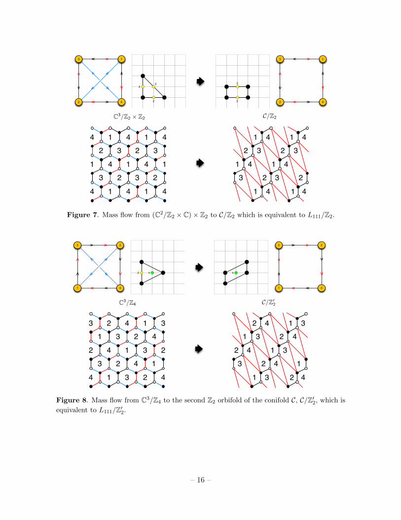
C/Z2C3/Z2 Z2

Figure 7. Mass flow from (C2/Z2 × C)× Z2 to C/Z2 which is equivalent to L111/Z2.

1

2

23

4 1

4 1 3

3 2 4

4 1 3 2

3 2 4 1

3 2 4

1

2

2

1

4 1 3

3 2 4

4 1 3

3 2 4 1

3 2 4

2 4 4

3 2

1 4

3 2

1 4

C3/Z4 C/Z02

Figure 8. Mass flow from C3/Z4 to the second Z2 orbifold of the conifold C, C/Z′2, which is

equivalent to L111/Z′2.

– 16 –

6

5

52

4 1

4 1 6

3 2 5

4 1 6 3

3 2 5 4

6 3 2

6

5

52

1

4 1 6

3 2 5

4 1 6 3

3 2 5 4

6 3

3 6

3

2

2 6

2

C3/Z3 Z2 PdP3c

52

3

1

4

6

52

3

1

4

6

Figure 9. Mass flow from (C2/Z3 × C)× Z2 to L121/Z2 also known as PdP3c.

2

24

3 4

3 4 2

5 6

3 4 2 3

5 6 5

2 3 4

7

71

1

71

2

24

4

3 4 2

5 6

3 4 2 3

5 6 5

2 3

71

71

71

3 6

3

2

3 6

2

PdP4b PdP4a

7

1

2

6

4

3

5

7

1

2

6

4

3

5

Figure 10. Mass flow from PdP4b to PdP4a.

– 17 –

4

8

87

1 2

1 2 3

5 6 7

1 2 3 4

5 6 7 8

3 4 5

4

8

2

1 2 3

5 6 7

1 2 3 4

5 6 7 8

3 4 5

6 8

4

4 8

3 8

3 8

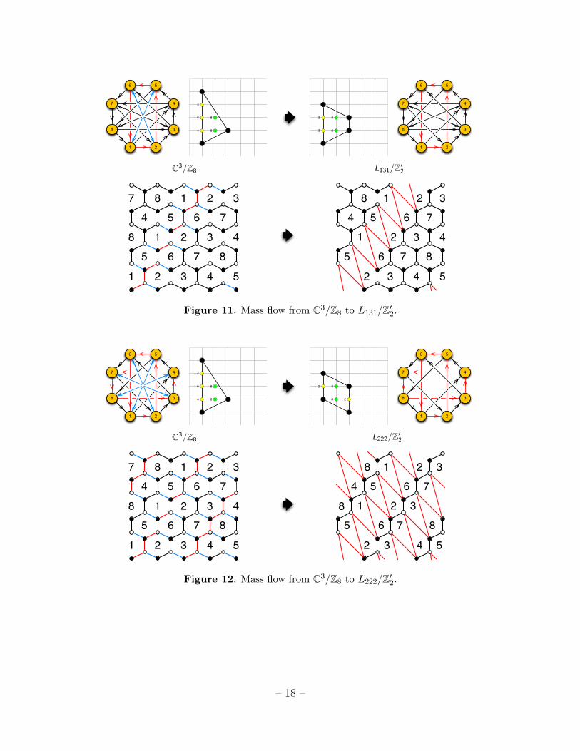
C3/Z8 L131/Z02

8

1

5

2

6

3

7 4

8

1

5

2

6

3

7 4

Figure 11. Mass flow from C3/Z8 to L131/Z′2.

4

8

87

1 2

1 2 3

5 6 7

1 2 3 4

5 6 7 8

3 4 5

4

8

8

2

1 2 3

5 6 7

1 2 3

5 6 7 8

3 4 5

6 8

4

4 8

2 8

8 2

C3/Z8 L222/Z02

8

1

5

2

6

3

7 4

8

1

5

2

6

3

7 4

Figure 12. Mass flow from C3/Z8 to L222/Z′2.

– 18 –

4 R-symmetry, a-maximization and volume minimization

It is well known that the R-symmetry in the SU(2, 2|1) superconformal algebra of any

4d SCFT is exactly and uniquely determined by an extremization procedure [34]. The

exact superconformal R-symmetry maximizes the expression of the central charge a

[35] in terms of ’t Hooft anomalies

a =3

32(3TrR3 − TrR) , (4.1)

where the right-hand side is considered for any non-anomalous U(1) R-symmetry Rtrial

rather than just the superconformal one R.

In practice, one can start from a linear combination Rtrial = R0 +∑

I αiJi of

a fiducial non-anomalous R-symmetry generator R0 with the non-anomalous Abelian

global symmetry generators Ji, compute atrial and maximize with respect to αi. The

maximum of atrial is the central charge a of the SCFT. As a corollary, one can argue

that the central charge a decreases along RG flows. Indeed, relevant deformations

break some of the flavor symmetries so, in the absence of accidental symmetries, the

extermination in the IR under a subset of the αi’s leads to a smaller value aIR < aUV [34].

For theories in this class, a generalization of (4.1) has been introduced by [36] which can

be used away from the endpoints of RG flows. The resulting a-function monotonically

decreases along the entire RG flow if there are no accidental symmetries. However, the

RG flows under consideration in this paper exhibit accidental symmetries in the IR so

we cannot use the a-function to study the RG flow locally in the energy scale.7 We will

content ourselves with checking that aIR < aUV in all RG flows under consideration,

consistently with the a-theorem.

We stress that, to obtain the correct superconformal R-charge and a central charge

of the infrared SCFT, it is essential to take into account the accidental mesonic sym-

metry that is made manifest by the field redefinitions discussed in the previous section.

Maximizing only with respect to the mesonic symmetries that are present all along the

RG flows generically leads to the wrong answer, as expected on general grounds [34].

The connection with toric geometry and volume minimization was first pointed out

in [38], where it is shown that the Reeb vector and the volume of a Sasaki-Einstein

metric on the base of an n-dimensional toric Calabi-Yau cone may be computed by

minimizing a function Z which depends only on the toric data. For toric CY 3-folds,

the Reeb vector and the volume correspond to the superconformal R-symmetry and

the inverse of the central charge c = a of the holographic dual SCFT, respectively.

7One could use the a-function employed in the proof of the a-theorem by [37], but that requires

computing a scattering amplitude rather than a ’t Hooft anomaly.

– 19 –

Agreement between volume minimization and a-maximization for toric SCFT’s was

shown in [39] and later generalized to non-toric cases in [30, 40]. In the present inves-

tigation, we are interested in relevant mass deformations which, despite breaking the

toric condition, lead to RG flows both of whose endpoints are toric SCFT’s. We will

show that for each of the considered flows, VIR > VUV (or equivalently aIR < aUV using

a-maximization).

4.1 Volume minimization

We have already recalled that the mesonic moduli space is a Calabi-Yau cone C(X)

over a Sasaki-Einstein 5-manifold X [12, 41]. Let us compute first the volumes VUVand VIR of X at the two ends of the mass flow. According to holography, the volumes

V and the Reeb vector can be found by extremizing a volume function Z introduced in

[38]. The function Z is encoded in the Hilbert series which counts chiral gauge invariant

operators of the SCFTs. More precisely, introducing a fugacity tα = e−µrα for each of

the GLSM field pα associated to the CY singularity, the volume function Z is defined

as

Z(rα;M) = limµ→0

µ3g(e−µrα ;M) . (4.2)

Note that we are overparametrizing the space of R-charges: the volume function is

invariant under

rα → rα +c−3∑i=1

si(Qt)iα , (4.3)

since the mesonic moduli space is the Kahler quotient (2.8). The freedom (4.3) can

be used to fix c − 3 of the c perfect matching variables. In addition, because each

perfect matching variables appears exactly once in each superpotential term, which

has R-charge 2, the R-charges rα satisfy∑α

rα = 2 . (4.4)

The remaining 2-dimensional subspace corresponds to the mixing of the R-symmetry

with mesonic symmetries. Extremizing Z with respect to rα over this subspace leads

to the volume

V (M) = Ω ·min Z(rα;M) , Ω =

(2π

3

)3

, (4.5)

where we have introduced a suitable normalization factor Ω. The R-charges of the

SCFT are obtained from the values of rα extremizing Z. For example for M = C3

Z =1

r1r2(2− r1 − r2)⇒ VS5 = π3 r1 = r2 =

2

3(4.6)

– 20 –

as expected for the N = 4 theory. In the following paragraphs, we compute the volume

of the SCFTs at the two ends of the mass flows under consideration in this paper.

Volumes for C2/Zn × C→ Lk,n−k,k and their orbifolds

We start by considering the flow starting from C2/Zn × C. The volume of an orbifold

of a manifold M is simply the volume of M divided by the order of the group. For

S5/Zn one then finds

VS5/Zn =π3

n. (4.7)

On the other hand the volume of La,b,a can be obtained by extremizing the volume

function8

ZLa,b,a =br1 + ar2 + ar3 + br4

(br1 + ar2)(ar3 + br4)(r2 + r3)(r1 + r4), (4.8)

with

r1 + r2 + r3 + r4 = 2

(r1, r2, r3, r4) ∼ (r1, r2, r3, r4) + (−a, b,−b, a)s .(4.9)

Extremizing along the 2-dimensional subspace corresponding to mixing with the mesonic

symmetries, one finds

VLa,b,a =4π3

27a2b2

[(2b− a)(2a− b)(a+ b) + 2(a2 + b2 − ab) 3

2

](4.10)

Taking a = k and b = n − k, one can check that VLk,n−k,k > VS5/Zn for all n > 0 and

k = 1, . . . ,[n2

](which covers the entire range because La,b,a = Lb,a,b). As expected, the

volume of the Sasaki-Einstein manifold increases along the RG flow. Similarly, for the

volumes of C3/Zn×Z2 and C3/Z2n one finds half the result (4.7) since the order is twice

as larger. On the other hand, the endpoints of the flows starting on these singularities

are Z2 orbifolds of Lk,n−k,k and therefore the volumes are just half of those of Lk,n−k,k.

Again the volumes increase along the flow as expected.

8This expression follows easily from the toric description for La,b,a: the toric diagram has vertices

w1 = (0, 0), w2 = (1, 0), w3 = (1, a), w4 = (0, b). The charge matrix of the GLSM isQt = (−a, b,−b, a).

The singularity is the hypersurface xy = zawb in C4. The computation here agrees with the results in

[12, 41].

– 21 –

Volumes flow for PdP4b → PdP4a

Finally, for PdP4b one finds9

ZPdP4b=

3r1 + 2r2 + 4r3 + 12r4

(r3 + 3r4)(4r4 + r1)(2r3 + r2)(3r1 + 2r2), (4.11)

with

r1 + r2 + r3 + r4 = 2

(r1, r2, r3, r4) ∼ (r1, r2, r3, r4) + (−4, 6,−3, 1)s .(4.12)

The volume is given by the minimum

VPdP4b' 0.531049 Ω . (4.13)

In comparison, PdP4a has the volume function10

ZPdP4a = (4r21 + 2r2

2 + 6r1r2 + 16r1r3 + 8r1r4 + 12r1r5 + 12r2r3 + 5r2r4 + 8r2r5

+12r23 + 12r3r4 + 2r2

4 + 16r3r5 + 6r4r5 + 4r25)×

1

(2r1 + r2 + 2r3)(2r1 + 2r2 + r4)(r1 + 3r3 + r5)(r2 + 2r4 + 2r5)(2r3 + r4 + 2r5),

(4.14)

with

r1 + r2 + r3 + r4 + r5 = 2

(r1, r2, r3, r4, r5) ∼ (r1, r2, r3, r4, r5) + (2,−2,−1, 0, 1)s1 + (1, 0,−1,−2, 2)s2 ,(4.15)

leading to the volume

VPdP4a ' 0.595008 Ω . (4.16)

The volume of the Sasaki-Einstein manifold increases in agreement with the holographic

a-theorem.

9The toric diagram of PdP4b has vertices w1 = (0, 0), w2 = (1, 0), w3 = (2, 1), w4 = (0, 3). The

charge matrix of the associated GLSM is Qt = (−4, 6,−3, 1). PdP4b is a non-complete intersection.

The computation here agrees with the results in [33].10The toric diagram of PdP4a has vertices w1 = (0, 2), w2 = (1, 2), w3 = (0, 0), w4 = (2, 1) and

w5 = (2, 0). The charge matrix of the associated GLSM is Q =

(2 −2 −1 0 1

1 0 −1 −2 2

). The computation

here agrees with the results in [33].

– 22 –

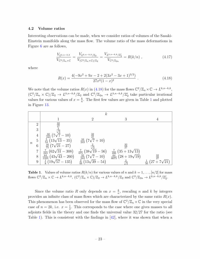
4.2 Volume ratios

Interesting observations can be made, when we consider ratios of volumes of the Sasaki-

Einstein manifolds along the mass flow. The volume ratio of the mass deformations in

Figure 6 are as follows,

VLk,n−k,k

VC2/Zn×C=

VLk,n−k,k/Z2

V(C2/Zn×C)/Z2

=VLk,n−k,k/Z′2VC2/Z2n

= R(k/n) , (4.17)

where

R(x) =4(−9x2 + 9x− 2 + 2(3x2 − 3x+ 1)3/2)

27x2(1− x)2. (4.18)

We note that the volume ratios R(x) in (4.18) for the mass flows C2/Zn×C→ Lk,n−k,k,

(C2/Zn × C)/Z2 → Lk,n−k,k/Z2 and C3/Z2n → Lk,n−k,k/Z′2 take particular irrational

values for various values of x = kn. The first few values are given in Table 1 and plotted

in Figure 13.

k

1 2 3 4

n

2 3227

3 2√3

4 32243

(7√

7− 10)

3227

5 554

(13√

13− 35)

10243

(7√

7 + 10)

6 1675

(7√

21− 27)

2√3

3227

7 7243

(62√

31− 308)

7675

(38√

19− 56)

7486

(35 + 13

√13)

8 641323

(43√

43− 260)

32243

(7√

7− 10)

646075

(28 + 19

√19)

3227

9 18

(19√

57− 135)

249

(13√

39− 54)

2√3

150

(27 + 7

√21)

Table 1. Values of volume ratios R(k/n) for various values of n and k = 1, . . . , [n/2] for mass

flows C2/Zn × C→ Lk,n−k,k, (C2/Zn × C)/Z2 → Lk,n−k,k/Z2 and C3/Z2n → Lk,n−k,k/Z′2.

Since the volume ratio R only depends on x = kn, rescaling n and k by integers

provides an infinite class of mass flows which are characterized by the same ratio R(x).

This phenomenon has been observed for the mass flow of C2/Zn×C in the very special

case of n = 2k, i.e. x = 12. This corresponds to the case where one gives masses to all

adjoints fields in the theory and one finds the universal value 32/27 for the ratio (see

Table 1). This is consistent with the findings in [42], where it was shown that when a

– 23 –

N = 2 SCFT flows to a N = 1 SCFT by masses given to all adjoint fields, the central

charges a and c before and after the flow take the ratio R = 3227

.

Interestingly, the ratio R = 3227

is the maximum value achieved by the flows con-

sidered in this paper. Here we have extended this observation beyond masses given to

adjoints and with the result that there is an infinite number of ‘mass flow classes’

characterized by their ratios R(x) with x ∈ [12, 1). This is shown for mass flows

C2/Zn × C → Lk,n−k,k, (C2/Zn × C)/Z2 → Lk,n−k,k/Z2 and C3/Z2n → Lk,n−k,k/Z′2.

It would be interesting to study this phenomenon further in future work.

5

10

15

20

2

1 10

5

k

n

x

R(x)

0.5 0.6 0.7 0.8 0.9 1.01.00

1.05

1.10

1.15

1.201.20

1.15

1.10

1.05

0.6 0.7 0.8 0.9 1.01.00

0.5

Figure 13. Volume ratio plot for mass flows C2/Zn × C → Lk,n−k,k, (C2/Zn × C)/Z2 →Lk,n−k,k/Z2 and C3/Z2n → Lk,n−k,k/Z′2. Different colors correspond to different values of the

volume ratio R(k/n) in the left plot. The right plot shows the correspondence between the

volume ratio R(x) and the flow parameter x = kn .

5 Mass deformations as complex structure deformations

and Hilbert series

The introduction of masses deforms the superpotential of the toric SCFT and therefore

its F-term relations. In this section, we show how this results into a complex structure

deformation of the underlying singularity by looking directly at the algebraic descrip-

tion of the mesonic moduli space and its Hilbert series, rather than performing field

redefinitions of the microscopic fields.

– 24 –

Let us consider the simplest flow C2/Zn × C → Lk,n−k,k as an illustration of the

general phenomenon. The gauge invariant mesonic operators are given by

x =n∏i=1

Xi,i+1 , y =n∏i=1

Xi,i+1 , wi = Xi,i+1Xi+1,i , φi (5.1)

satisfying

x y =n∏i=1

wi . (5.2)

After the mass deformation the relations among these operators that follow from their

definition and the F-term equations become11

φi = z , ∀i = 1, ..., n

w2i−2 − w2i−1 +mφ2i−1 = w2i−1 − w2i −mφ2i = 0 , i = 1, ..., k

wi−1 − wi +mφi = 0 , i = 2k + 1, ..., n . (5.3)

The solution can be written as

w2i−1 −mz = w2i = w i = 1, ..., k

wi = w i = 2k + 1, ..., n (5.4)

while the relation (5.2) becomes

x y = (w +mz)k wn−k . (5.5)

If m = 0, (5.5) reduces to the algebraic description of C2/Zn in terms of the generators

x, y and w, which is in a product with the C plane generated by z. If m 6= 0, the

equation which describes the singularity is deformed, and the symmetry acting on x,

y, z and w by complex rescalings is broken from C∗3 to C∗2. However, we can change

variable z to z = mz + w in order to recast (5.5) into

x y = zk wn−k . (5.6)

This is nothing but the defining equation of the cone over Lk,n−k,n, which enjoys the

full toric C∗3 symmetry. We see that as soon as the mass parameter is turned on,

the complex structure of the mesonic moduli space becomes that of the cone over

Lk,n−k,n, which is associated to the infrared SCFT. This fact is well known for the

11We restrict to the mesonic branch of the moduli space, where the adjoint fields are equal. This

condition is not satisfied on the branches of the moduli space corresponding to the regular D3-brane

splitting into fractional D3-branes.

– 25 –

flow C2/Zn × C→ Lk,n−k,k [9], although here we have emphasized the choices of mass

parameters that lead to a toric mesonic moduli space for the mass-deformed theory (or

equivalently in the infrared). We claim that this phenomenon, which was studied from

the dual supergravity perspective in [43], applies to all the mass flows described in this

paper even in the cases where the singularities are not complete intersections.

There are two ways to understand why the mesonic moduli space becomes the

toric Calabi-Yau threefold associated to the infrared field theory as soon as the mass

deformation is turned on. The first way is to analyze directly the F -term equations, as

reviewed in section §3 and detailed in Appendix A. Since imposing F -term equations ef-

fectively integrates out massive fields, the mesonic moduli spaces of the mass-deformed

UV theory and of the low energy theory obtained by integrating out the massive fields

coincide. Using the light matter fields of the UV theory only manifests a U(1)2 sym-

metry in the mesonic moduli space, because the mass deformation explicitly breaks a

U(1) factor of the toric U(1)3 of the UV CFT. However a change of variables (3.3)

recasts the low energy superpotential in toric form, making it clear that the mesonic

moduli space of the IR CFT (or, equivalently, of the mass-deformed UV CFT) is a toric

Calabi-Yau threefold.

An alternative and more general perspective on this point, even though it misses

the accidental symmetry, is offered by the Hilbert series of the mesonic moduli space of

the Abelian quiver gauge theory [28, 29]. In this section we work with the matter fields

of the quiver gauge theory subject to F -term equations, rather than with the perfect

matching variables appearing in (2.9), that are associated to the GLSM description

of the toric Calabi-Yau, which has a larger gauge group and no superpotential. The

Hilbert series of the mesonic moduli space counts gauge invariant chiral operators,

weighted according to their charges under the global symmetry. It is given by a Molien

formula similar to (2.9), but now the integral is over the gauge group of the quiver

gauge theory. Chiral multiplets Φ in the quiver contribute to the integrand factors

(1 − tΦ)−1, where tΦ is the weight of Φ under the global and gauge symmetry group,

whereas F -term equations contribute to the numerator. To proceed, we note that the

F -term equations for the massive fields are linear in the massive fields and can be solved

independently of the other equations. So the F -term of a massive field X contributes

a factor (1− t ∂W∂X

) to the numerator of the integrand.

We start from the Hilbert series of the mesonic moduli space of the toric UV theory,

which depends on three fugacities associated to the U(1)3 non-baryonic symmetry. All

the weights above are monomials in such fugacities and the fugacities for the gauge

group. The first effect of the mass deformation on the Hilbert series of the mesonic

moduli space of the UV theory is to unrefine it with respect to the non-baryonic sym-

metry which is broken by the mass terms: the fugacity associated to the broken U(1)

– 26 –

symmetry is set to 1. Secondly, in the Molien integrand the F -term of a field X ap-

pearing in a superpotential mass term mXY exactly cancels the contribution of the

partner field Y ,1− t ∂W

∂X

1− tY= 1 , (5.7)

because ∂W∂X

and Y are forced by the mass term to have the same quantum numbers

under the unbroken symmetries.

Since massive fields and their F -term equations cancel out in the Hilbert series,

we conclude that the Hilbert series of the mass-deformed UV theory coincides with the

Hilbert series of the IR theory, unrefined with respect to the accidental symmetry. In

particular, a necessary condition for two toric Calabi-Yau threefolds (complete inter-

sections or not) to be related by a mass flow is that their Hilbert series coincide under

a certain unrefinement. This is a restrictive constraint, because it implies a bijection

between spectra of holomorphic functions.

As an example, let us return to the flows C2/Zn × C → Lk,n−k,k. For C2/Zn × C,

parametrized by (x, y, w, z) subject to xy = wn, the refined Hilbert series is

g(t;C2/Zn × C) = PE [tx + ty + tw + tz − tnw] , with txty = tnw . (5.8)

Unrefining with respect to the broken U(1) symmetry sets tz = tw and yields

g(t;C2/Zn × C)|tz=tw = PE[tx + ty + 2tw − tnw] , with txty = tnw . (5.9)

For the cone over Lk,n−k,k, parametrized by (X, Y,W,Z) subject to XY = ZkW n−k,

the refined Hilbert series is

g(T ;Lk,n−k,k) = PE[tX + tY + tW + tZ − tkZtn−kW

], with tXtY = tkZt

n−kW . (5.10)

Unrefining with respect to the accidental U(1) symmetry sets tZ = tW and yields

g(T ;Lk,n−k,k)|tZ=tW = PE [tX + tY + 2tW − tnW ] , with tXtY = tnW , (5.11)

which indeed coincides with (5.9) if (tX , tY , tW ) = (tx, ty, tw).

6 The string amplitude

In the last section we give some evidence for the interpretation of mass deformations

as complex deformations of the UV Calabi-Yau cone. This suggests that mass defor-

mations can be realized in String Theory by turning on 3-form NSNS and RR fluxes.

Here we support this identification, by computing the mass couplings of 3-form fluxes

– 27 –

to open string fermion bilinears. The mass couplings will be extracted from the three

point functions on a disk involving the insertion of two open and one closed string

vertex operators.12

We focus on the C2/Zn×C case. The generalization to the other orbifold theories

under consideration here is straightforward since the orbifold groups always contain an

N = 2 element, i.e. an element leaving invariant one complex plane, let us say X3.

Turning on a flux belonging to this sector will give mass to the scalar field Φ3. The only

difference with the N = 2 setup is that for N = 1 orbifold theories, the orbifold group

acts non-trivially on Φ3 and therefore Chan-Paton indices should be taken off-diagonal

leading to bifundamental rather than adjoint representations.

Open string vertices can be chosen among the gaugino and the fermions in the

bifundamental matter

VΛ0 = Λ0α e−ϕ

2 Sα Σ0 (x)

VΛI = ΛIα e−ϕ

2 Sα ΣI (x) . (6.1)

The gaugino field is described by block diagonal matrix Λ0α while matter fermions are

given by off-diagonal matrices ΛIα with non-trivial Na×Na+aI block components. There

are two choices for the closed string fields depending on whether we consider fluxes

coming from the untwisted or twisted sectors. The result in the untwisted sector can

be borrowed from that in flat space-time [44] after Chan-Paton matrices are properly

projected. For convenience of the reader, we review the results here. The closed string

vertices for RR and NSNS 3-form fluxes in the untwisted sector are given by

VF = (FR0)AB e−ϕ

2 Sα ΣA(z) e−ϕ2 Sα ΣB(z) + (FR0)AB e−

ϕ2C α ΣA(z) e−

ϕ2 Cα ΣB(z)

VH = ∂m(BR0)np ψmψn(z)e−ϕψp(z) (6.2)

with A = 0, . . . 3 upper and lower indices labeling the L- and R-moving spinor rep-

resentations of the R-symmetry group SO(6), and R0 = −1, R0 = Γ4 . . .Γ9 are the

reflection matrices relating left to right moving modes of the strings. Explicitly

(FR0)AB = ∗Fmnp(Σmnp)AB (BR0)np = −Bnp (6.3)

where m = 1, ..6 runs over the vector of SO(6). Finally internal spin fields can be

written in the bosonized form

Σ0 = ei2

(ϕ1+ϕ2+ϕ3) ΣI = e−i2

(ϕ1+ϕ2+ϕ3−2ϕI) Sα = e±i2

(ϕ4+ϕ5) Cα = e±i2

(ϕ4−ϕ5)

(6.4)

12M. B, J. F. M. and D. R. P. would like to acknowledge stimulating discussions on this issue with

G. Inverso and L. Martucci.

– 28 –

and upper indices are given by their complex conjugates. Collecting all pieces and

plugging them into the disk amplitudes 〈VF,HΛAΛB〉, one finds the three point couplings

[44]

L3−form = 2π3!GIASDmnp (Σmnp)AB TrΛαA ΛB

α + h.c. (6.5)

where GIASD = ∗F − τH is the imaginary anti self-dual part of the three-form field13

G = F − τH . (6.6)

In components, after keeping only Zn-invariant components of the fluxes, one finds

12πLuntw = G(3,0)TrΛα0 Λ0

α +G(1,2)TrΛα3 Λ3α . (6.7)

Notice that the first term breaks supersymmetry since it gives mass to the gaugino. On

the other hand, a flux of (1,2) type generates a supersymmetric mass for the adjoint

fermions Λ3.

Now, let us consider the twisted closed string spectrum. Denoting by θI = (θ, 1−θ, 0), θ ∈ 1

nZ, the bosonic twists, the relevant vertex for NSNS and RR field strengths

can be written as

VH,tw = H e−ϕ2∏I=1

σθIeiϕIθI (z)e−iϕ3

2∏I=1

σθIe−iϕIθI (z)

VF,tw = F e−ϕ2 e−

iϕ32 Sα

2∏I=1

σθIeiϕI( 1

2−θI)(z)e−

ϕ2 e−

iϕ32 Sα

2∏I=1

σθIe−iϕI( 1

2−θI)(z) (6.8)

with σθI the bosonic twist fields. The vertices (6.8) are massless for any choice of θ

since left and right moving conformal dimensions add up to one.14 Terms combine

again into imaginary anti-self-dual combinations generating the bilinear couplings

12πLΘh−tw = G(1,2),hTr

(ΘhΛα3 Λ3

α

). (6.9)

Comparing (6.9) with (6.7), one notices that an untwisted 3-form flux produces identical

masses for all the adjoint hypermultiplets while fluxes from the twisted sector can be

used to tune mass differences. The flows studied in this paper are then induced by

NSNS/RR 3-form fluxes coming from twisted sectors localized at the singularities.

In the following we present the derivation of this coupling for the RR vertex. A

similar computation can be performed for the NSNS field.

13We take τ = igs

.14The dimensions of the various fields are [e−ϕ/2] = 3

8 , [e−ϕ] = 12 , [eiqϕi ] = q2

2 , [σθI ] = θI2 (1 − θI),

[eiθ] = θ2

2 .

– 29 –

6.1 The RR amplitude

Let us compute the coupling FΛα3Λ3α. The relevant disk amplitude (at zero momenta)

is ∫dz2 〈VΛ3(z1)VΛ3(z2)VF (z3, z4)〉 = FΛ3

α1Λ3α2εα3α4 Aα1α2α3α4 (6.10)

with

Aα1α2α3α4 =

∫dz2

⟨ce−

ϕ2 Sα1 Σ3 (z1)e−

ϕ2 Sα2 Σ3 (z2)

× ce−ϕ2 e−iϕ32 Sα3

2∏I=1

σθIeiϕI( 1

2−θI)(z3)ce−

ϕ2 e−iϕ3

2 Sα4

2∏I=1

σθIe−iϕI( 1

2−θI)(z4)

⟩.

The various contributions are

〈e−ϕ2 (z1)e−ϕ2 (z2)e−

ϕ2 (z3)e−

ϕ2 (z4)〉 = (z12z13z14z23z24z34)−1/4

〈e iϕ32 (z1)eiϕ32 (z2)e−

iϕ32 (z3)e−

iϕ32 (z4)〉 =

(z12z34

z13z24z14z23

)1/4

〈e i2 (ϕ1+ϕ2)(z1)ei2

(ϕ1+ϕ2)(z2)2∏I=1

σθIeiϕI( 1

2−θI)(z3)

2∏I=1

σθIe−iϕI( 1

2−θI)(z4)〉 =

(1

z12z34

) 12

〈Sα1(z1)Sα2(z2)Sα3(z3)Sα4(z4)〉 =

(z14z23z13z24

z12z34

)1/2 [εα1α3εα2α4

z13z24

+εα1α4εα2α3

z14z23

]〈c(z1)c(z3)c(z4)〉 = z13z34z41 . (6.11)

Contracting with εα3α4 , one finds15

εα3α4Aα1α2α3α4 = εα1α2

∫|w|=1

dw

w= 2πi εα1α2 (6.12)

with w = z24z13z14z23

the complex cross ratio. Plugging (6.12) into (6.10) one finds the

F-contribution to the coupling (6.9).

A similar computation can be performed for untwisted R-R fluxes. The relevant

disk amplitude (at zero momenta) reads

AKLIJ =

∫dz2

⟨ce−

ϕ2 Sα ΣI (z1)e−

ϕ2 Sα ΣJ (z2)ce−

ϕ2 e−iϕ3

2 C α ΣK (z3)ce−ϕ2 e−iϕ3

2 Cα ΣL (z4)⟩

= δ(I(Kδ

J)L)

∫|w|=1

dw

w= 2πi δ

(I(Kδ

J)L) (6.13)

leading to (6.7).

15 Here we write dz2z34z23z24

= dww with |w| = 1.

– 30 –

7 Conclusions

In this paper we have shown that brane tiling methods can be used to efficiently study

RG flows between toric quiver gauge theories triggered by mass terms. Even though

mass terms break the U(1)3 toric symmetry of the UV superconformal field theory and

cannot be described by nodes in a brane tiling, for judicious choices of the masses with

pairs of equal and opposite mass parameters it is possible to flow to another supercon-

formal toric quiver gauge theory in the IR. The IR toric U(1)3 non-baryonic symmetry

involves an accidental mesonic symmetry which appears once the massive fields are

integrated out. The accidental symmetry is manifested by a change of variables for

the light fields which recasts the superpotential in toric form. The endpoints of such

renormalization group flows can be easily visualized by performing a certain move on

the brane tiling associated to the UV fixed point. The effect of this move is to reverse

the winding numbers of a particular zig-zag path made of those massless fields which

appear in two toric superpotential terms with massive fields.

Although the mass-deformed theory does not have a U(1)3 non-baryonic symmetry

along the RG flow, its mesonic moduli space is actually a toric Calabi-Yau cone: this

is nothing but the Calabi-Yau cone associated to the IR fixed point, since the U(1)

charges of F -terms are independent of the RG scale. We have shown that the volumes

of the Sasaki-Einstein bases of the singularity cones always increase along the flows

from UV to IR, in agreement with the holographic a-theorem. Interestingly, for flows

starting from an orbifold singularity the ratio between IR and UV volumes depends

only on the order of the group and the number of massive deformations with maximum

value 32/27 matching the universal value explained in [42] for flows from N = 2 to

N = 1 SCFT where all adjoint fields get masses. This universal value is also achieved

for flows involving massive bifundamental matter.

The toric Calabi-Yau cones associated to the UV and IR fixed points are related

by a complex deformation. We have shown the relation between UV and IR toric

Calabi-Yau cones in a simple class of examples, in terms of the algebraic description

of the singularity and its Hilbert series. The introduction of a mass term has the net

effect of partially unrefining the Hilbert series of the mesonic moduli space of the UV

theory with respect to the global symmetry broken by the mass term, and the Hilbert

series of the mass-deformed UV theory coincides with that of the Hilbert series of the

IR theory, unrefined with respect to the accidental symmetry.

The mass deformation is induced by the presence of an imaginary-self-dual 3-form

fluxes in the twisted sector. We supported this identification by an explicit computation

of the disk amplitude involving a closed 3-form vertex from the twisted sector and two

open string fermions.

– 31 –

Analogously to our study of mass deformations, it would be interesting to analyze

the effect of other relevant or marginal deformations [30] and identify the source of the

deformation from the bulk point of view. The results of this paper relate gauge the-

ories on non-orbifold singularities like Laba (or orbifolds of them) to orbifold theories.

In orbifold theories, one has complete control of the dynamics from the world-sheet

vantage point. One can not only compute mass terms generated by twisted bulk fluxes,

as done in section §6, but also superpotentials and other interactions in the effective

action dynamically generated by ‘gauge’ or ‘exotic’ instantons [45–51]. It would be

interesting to extend the results of this paper to superconformal unoriented theories

that emerge from D3-branes at orientifold singularities [52] and exploit the worldsheet

description in the UV to learn about the strong coupling dynamics of the non-orbifold

theories in the IR. Given their possible role in embedding (supersymmetric) extensions

of the Standard Model, configurations of unoriented D-branes at Calabi-Yau singular-

ities certainly deserve a systematic analysis starting from the toric case along the lines

of [53–56].

Acknowledgements

We kindly acknowledge discussions with A. Amariti, C. Bachas, M. Bertolini, S. Franco,

A. Mariotti, D. Orlando, G. Inverso and L. Martucci. We thank the following institutes

for their kind hospitality during the completion of this work: the Theoretical Physics

groups at Imperial College London (MB, JFM, DRP, R-KS), Queen Mary University

of London (MB), Padua University (R-KS), the University of Rome Tor Vergata (SC,

DRP) and the Mathematical Institute of the University of Oxford (JFM); the Simons

Center of Geometry and Physics in Stony Brook (AH, R-KS), the Galileo Galilei Insti-

tute in Florence (SC), the Royal Society at Chicheley Hall (MB, SC, AH, R-KS) and

the ICMS in Edinburgh (MB, SC, AH, JFM, R-KS). The work of MB and JFM is par-

tially supported by the ERC Advanced Grant n. 226455 “Superfields” and was initiated

while MB was visiting Imperial College and largely carried on while MB was holding

a Leverhulme Visiting Professorship at QMUL. The work of JFM is also supported by

the Engineering and Physical Sciences Research Council, grant numbers EP/I01893X/1

and EP/K034456/1. The research of DRP was supported by the Padova University

Project CPDA119349 and by the MIUR-PRIN contract 2009-KHZKRX.

A Details of the flows

In this appendix we collect the details of the mass flows described in section §2. For

each case we list the starting and end superpotentials, the mass deformation, the F-

– 32 –

term conditions and the field redefinitions.

A.1 C2/Zn × C to Lk,n−k,k

Superpotentials and mass terms:

WC2/Zn×C =n∑i=1

φi (Xi,i−1Xi−1,i −Xi,i+1Xi+1,i)

∆W =m

2

k∑i=1

(φ2

2i−1 − φ22i

)(A.1)

WLk,n−k,k =k∑i=1

(X ′2i−1,2iX

′2i,2i−1X2i−1,2i−2X2i−2,2i−1 −X ′2i,2i−1X

′2i−1,2iX2i,2i+1X2i+1,2i

)+

n∑i=k+1

φ′i (Xi,i−1Xi−1,i −Xi,i+1Xi+1,i)

where subscripts i are understood modulo n.

F-term and field redefinitions:

φ2i−1 =1

m(X2i−1,2iX2i,2i−1 −X2i−1,2i−2X2i−2,2i−1)

φ2i =1

m(X2i,2i−1X2i−1,2i −X2i,2i+1X2i+1,2i)

φj = φ′j −1

2m(Xj,j+1Xj+1,j +Xj,j−1Xj−1,j)

X2i−1,2iX2i,2i−1 = mX ′2i−1,2iX′2i,2i−1 (A.2)

with i = 1, . . . , k and j = 2k + 1, . . . , n.

– 33 –

A.2 (C2/Zn × C)/Z2 to Lk,n−k,k/Z2

The superpotential of the (C2/Zn × C)/Z2 model is given by

W(C2/Zn×C)/Z2=

n∑i=1

[X2i−1,2i (X2i,2i+2X2i+2,2i−1 −X2i,2i−3X2i−3,2i−1)

+X2i,2i−1 (X2i−1,2i+1X2i+1,2i −X2i−1,2i−2X2i−2,2i)]

∆W = m2k∑i=1

(−1)iX2i−1,2iX2i,2i−1 (A.3)

WLk,n−k,k/Z2=

n∑i=2k+1

[X ′2i−1,2i (X2i,2i+2X2i+2,2i−1 −X2i,2i−3X2i−3,2i−1)

+ X ′2i,2i−1 (X2i−1,2i+1X2i+1,2i −X2i−1,2i−2X2i−2,2i)]

+k∑i=1

X ′4i−3,4i−1 (X4i−1,4i+1X4i+1,4iX4i,4i−3 −X4i−1,4i−2X4i−2,4i−5X4i−5,4i−3)

+k∑i=1

X ′4i−2,4i (X4i,4i+2X4i+2,4i−1X4i−1,4i−2 −X4i,4i−3X4i−3,4i−4X4i−4,4i−2)

where subscripts i are now understood modulo 2n.

F-terms and field redefinitions:

X2i−1,2i = (−1)i+1 1

m(X2i−1,2i+1X2i+1,2i −X2i−1,2i−2X2i−2,2i)

X2i,2i−1 = (−1)i+1 1

m(X2i,2i+2X2i+2,2i−1 −X2i,2i−3X2i−3,2i−1)

X2j−1,2j = X ′2j−1,2j −1

2m(X2j−1,2j−2X2j−2,2j +X2j−1,2j+1X2j+1,2j)

X2j,2j−1 = X ′2j,2j−1 −1

2m(X2j,2j+2X2j+2,2i−1 +X2j,2j−3X2j−3,2j−1)

X4l−3,4l−1 = mX ′4l−3,4l−1 , X4l−2,4l = mX ′4l−2,4l , (A.4)

with i = 1, . . . , 2k, j = 2k + 1, . . . , n and l = 1, . . . , k.

– 34 –

A.3 C3/Z2n to Lk,n−k,k/Z′2Superpotentials and mass terms:

WC3/Z2n=

2n∑i=1

Xi,i+1 (Xi+1,i+n+1Xi+n+1,i −Xi+1,i+nXi+n,i)

∆W = m

k∑i=1

(X2i−1,2i−1+nX2i−1+n,2i−1 −X2i,2i+nX2i+n,2i) (A.5)

WLk,n−k,k/Z′2 =n∑

i=2k+1

X ′i,i+n (Xi+n,i−1Xi−1,i −Xi+n,i+n+1Xi+n+1,i) +

+n∑

i=2k+1

X ′i+n,i (Xi,i+n−1Xi+n−1,i+n −Xi,i+1Xi+1,i+n) +

+k∑i=1

X ′2i−1,2i (X2i,2i−1+nX2i−1+n,2i−2X2i−2,2i−1 −X2i,2i+1X2i+1,2i+nX2i+n,2i−1) +

+k∑i=1

X ′2i−1+n,2i+n

(X2i+n,2i−1X2i−1,2i−2+nX2i−2+n,2i−1+n +

−X2i+n,2i+1+nX2i+1+n,2iX2i,2i−1+n

)(A.6)

with the subscripts understood modulo 2n.

F-terms and field redefinitions:

X2i−1,2i−1+n =1

m(X2i−1,2iX2i,2i−1+n −X2i−1,2i−2+nX2i−2+n,2i−1+n)

X2i−1+n,2i−1 =1

m(X2i−1+n,2i+nX2i+n,2i−1 −X2i−1+n,2i−2X2i−2,2i−1)

X2i,2i+n =1

m(X2i,2i+n−1X2i+n−1,2i+n −X2i,2i+1X2i+1,2i+n)

X2i+n,2i =1

m(X2i+n,2i−1X2i−1,2i −X2i+n,2i+1+nX2i+1+n,2i)

Xj,j+n = X ′j,j+n −1

2m(Xj,j+1Xj+1,j+n +Xj,j+n−1Xj+n−1,j+n)

Xj+n,j = X ′j+n,j −1

2m(Xj+n,j+n+1Xj+n+1,j +Xj+n,j−1Xj−1,j)

X2i−1,2i = mX ′2i−1,2i , X2i−1+n,2i+n = mX ′2i−1+n,2i+n , (A.7)

for i = 1, . . . , k and j = 2k + 1, . . . , n.

– 35 –

A.4 PdP4b to PdP4a

Superpotentials and mass terms:

WPdP4b= X12X25X51 +X13X34X41 +X14X47X71 +X24X45X52 +X35X56X63

− X12X24X41 −X13X37X71 −X14X45X51 −X23X35X52 −X25X56X62

+ X23X37X76X62 −X34X47X76X63

∆W = m (X14X41 −X25X52)

WPdP4a = X ′45 (X51X13X34 −X56X62X24) +X ′12 (X24X47X71 −X23X35X51) +

+ X ′63 (X35X56 −X34X47X76) +X ′37 (X76X62X23 −X71X13) . (A.8)

F-terms and field redefinitions:

X14 = +1

m(X12X24 −X13X34) , X41 = +

1

m(X45X51 −X47X71) ,

X25 =1

m(X24X45 −X23X35) , X52 = − 1

m(X51X12 −X56X62) , (A.9)

X37 = X ′37 −X34X47 , X63 = X ′63 −X62X23 , X12 = mX ′12 , X45 = mX ′45 .

References

[1] A. Hanany and A. Zaffaroni, On the realization of chiral four-dimensional gauge

theories using branes, JHEP 9805 (1998) 001, [hep-th/9801134].

[2] A. Hanany and K. D. Kennaway, Dimer models and toric diagrams, hep-th/0503149.

[3] S. Franco, A. Hanany, K. D. Kennaway, D. Vegh, and B. Wecht, Brane Dimers and

Quiver Gauge Theories, JHEP 01 (2006) 096, [hep-th/0504110].

[4] J. Davey, A. Hanany, and R.-K. Seong, Counting Orbifolds, JHEP 06 (2010) 010,

[arXiv:1002.3609].

[5] J. Davey, A. Hanany, and R.-K. Seong, An Introduction to Counting Orbifolds, Fortsch.

Phys. 59 (2011) 677–682, [arXiv:1102.0015].

[6] A. Hanany and R.-K. Seong, Symmetries of Abelian Orbifolds, JHEP 01 (2011) 027,

[arXiv:1009.3017].

[7] A. Hanany, V. Jejjala, S. Ramgoolam, and R.-K. Seong, Calabi-Yau Orbifolds and

Torus Coverings, JHEP 09 (2011) 116, [arXiv:1105.3471].

[8] I. R. Klebanov and E. Witten, Superconformal field theory on three-branes at a

Calabi-Yau singularity, Nucl.Phys. B536 (1998) 199–218, [hep-th/9807080].

[9] S. Gubser, N. Nekrasov, and S. Shatashvili, Generalized conifolds and 4-Dimensional

N=1 SuperConformal Field Theory, JHEP 9905 (1999) 003, [hep-th/9811230].

– 36 –

[10] M. Cvetic, H. Lu, D. N. Page, and C. Pope, New Einstein-Sasaki spaces in five and

higher dimensions, Phys.Rev.Lett. 95 (2005) 071101, [hep-th/0504225].

[11] S. Benvenuti and M. Kruczenski, From Sasaki-Einstein spaces to quivers via BPS

geodesics: L**p,q—r, JHEP 0604 (2006) 033, [hep-th/0505206].

[12] S. Franco et. al., Gauge theories from toric geometry and brane tilings, JHEP 01

(2006) 128, [hep-th/0505211].

[13] A. Butti, D. Forcella, and A. Zaffaroni, The Dual superconformal theory for L**pqr

manifolds, JHEP 0509 (2005) 018, [hep-th/0505220].

[14] D. R. Morrison and M. R. Plesser, Nonspherical horizons. 1., Adv.Theor.Math.Phys. 3

(1999) 1–81, [hep-th/9810201].

[15] A. M. Uranga, Brane configurations for branes at conifolds, JHEP 9901 (1999) 022,

[hep-th/9811004].

[16] K. Dasgupta and S. Mukhi, Brane constructions, conifolds and M theory, Nucl.Phys.

B551 (1999) 204–228, [hep-th/9811139].

[17] R. von Unge, Branes at generalized conifolds and toric geometry, JHEP 9902 (1999)

023, [hep-th/9901091].

[18] B. Feng, A. Hanany, and Y.-H. He, D-brane gauge theories from toric singularities and

toric duality, Nucl. Phys. B595 (2001) 165–200, [hep-th/0003085].

[19] B. Feng, A. Hanany, and Y.-H. He, Phase structure of D-brane gauge theories and toric

duality, JHEP 08 (2001) 040, [hep-th/0104259].

[20] S. Franco and D. Vegh, Moduli spaces of gauge theories from dimer models: Proof of

the correspondence, JHEP 0611 (2006) 054, [hep-th/0601063].

[21] A. Hanany and D. Vegh, Quivers, tilings, branes and rhombi, JHEP 10 (2007) 029,

[hep-th/0511063].

[22] O. Aharony, A. Hanany, and B. Kol, Webs of (p,q) 5-branes, five dimensional field

theories and grid diagrams, JHEP 01 (1998) 002, [hep-th/9710116].

[23] B. Feng, Y.-H. He, K. D. Kennaway, and C. Vafa, Dimer models from mirror symmetry

and quivering amoebae, Adv.Theor.Math.Phys. 12 (2008) 3, [hep-th/0511287].

[24] R. Bocklandt, Consistency conditions for dimer models, ArXiv e-prints (Apr., 2011)

[arXiv:1104.1592].

[25] N. Broomhead, Dimer models and Calabi-Yau algebras, ArXiv e-prints (Jan., 2009)

[arXiv:0901.4662].

[26] B. Feng, S. Franco, A. Hanany, and Y.-H. He, Symmetries of toric duality, JHEP 12

(2002) 076, [hep-th/0205144].

– 37 –

[27] B. Feng, S. Franco, A. Hanany, and Y.-H. He, Unhiggsing the del Pezzo, JHEP 08

(2003) 058, [hep-th/0209228].

[28] S. Benvenuti, B. Feng, A. Hanany, and Y.-H. He, Counting BPS operators in gauge

theories: Quivers, syzygies and plethystics, JHEP 11 (2007) 050, [hep-th/0608050].

[29] B. Feng, A. Hanany, and Y.-H. He, Counting Gauge Invariants: the Plethystic

Program, JHEP 03 (2007) 090, [hep-th/0701063].

[30] A. Butti, A. Zaffaroni, and D. Forcella, Deformations of conformal theories and

non-toric quiver gauge theories, JHEP 0702 (2007) 081, [hep-th/0607147].

[31] A. Hanany, P. Kazakopoulos, and B. Wecht, A new infinite class of quiver gauge

theories, JHEP 08 (2005) 054, [hep-th/0503177].

[32] A. Hanany, D. Orlando, and S. Reffert, Sublattice Counting and Orbifolds, JHEP 06

(2010) 051, [arXiv:1002.2981].

[33] A. Hanany and R.-K. Seong, Brane Tilings and Reflexive Polygons, Fortsch.Phys. 60

(2012) 695–803, [arXiv:1201.2614].

[34] K. A. Intriligator and B. Wecht, The Exact superconformal R symmetry maximizes a,

Nucl.Phys. B667 (2003) 183–200, [hep-th/0304128].

[35] D. Anselmi, D. Freedman, M. T. Grisaru, and A. Johansen, Nonperturbative formulas

for central functions of supersymmetric gauge theories, Nucl.Phys. B526 (1998)

543–571, [hep-th/9708042].

[36] D. Kutasov, New results on the ’a theorem’ in four-dimensional supersymmetric field

theory, hep-th/0312098.

[37] Z. Komargodski and A. Schwimmer, On Renormalization Group Flows in Four

Dimensions, JHEP 1112 (2011) 099, [arXiv:1107.3987].

[38] D. Martelli, J. Sparks, and S.-T. Yau, The geometric dual of a-maximisation for toric

Sasaki- Einstein manifolds, Commun. Math. Phys. 268 (2006) 39–65,

[hep-th/0503183].

[39] A. Butti and A. Zaffaroni, R-charges from toric diagrams and the equivalence of a-

maximization and Z-minimization, JHEP 11 (2005) 019, [hep-th/0506232].

[40] R. Eager, Equivalence of A-Maximization and Volume Minimization, JHEP 1401

(2014) 089, [arXiv:1011.1809].

[41] S. Benvenuti, S. Franco, A. Hanany, D. Martelli, and J. Sparks, An infinite family of

superconformal quiver gauge theories with Sasaki-Einstein duals, JHEP 06 (2005) 064,

[hep-th/0411264].

[42] Y. Tachikawa and B. Wecht, Explanation of the Central Charge Ratio 27/32 in

– 38 –

Four-Dimensional Renormalization Group Flows between Superconformal Theories,

Phys.Rev.Lett. 103 (2009) 061601, [arXiv:0906.0965].

[43] N. Halmagyi, K. Pilch, C. Romelsberger, and N. P. Warner, The Complex geometry of

holographic flows of quiver gauge theories, JHEP 0609 (2006) 063, [hep-th/0406147].

[44] M. Billo, L. Ferro, M. Frau, F. Fucito, A. Lerda, et. al., Non-perturbative effective

interactions from fluxes, JHEP 0812 (2008) 102, [arXiv:0807.4098].

[45] L. Ibanez and A. Uranga, Neutrino Majorana Masses from String Theory Instanton

Effects, JHEP 0703 (2007) 052, [hep-th/0609213].

[46] B. Florea, S. Kachru, J. McGreevy, and N. Saulina, Stringy Instantons and Quiver

Gauge Theories, JHEP 0705 (2007) 024, [hep-th/0610003].

[47] M. Cvetic, R. Richter, and T. Weigand, Computation of D-brane instanton induced

superpotential couplings: Majorana masses from string theory, Phys.Rev. D76 (2007)

086002, [hep-th/0703028].

[48] R. Argurio, M. Bertolini, G. Ferretti, A. Lerda, and C. Petersson, Stringy instantons at

orbifold singularities, JHEP 0706 (2007) 067, [arXiv:0704.0262].

[49] M. Bianchi, F. Fucito, and J. F. Morales, D-brane instantons on the T**6 / Z(3)

orientifold, JHEP 0707 (2007) 038, [arXiv:0704.0784].

[50] M. Bianchi and E. Kiritsis, Non-perturbative and Flux superpotentials for Type I

strings on the Z(3) orbifold, Nucl.Phys. B782 (2007) 26–50, [hep-th/0702015].

[51] M. Bianchi, F. Fucito, and J. F. Morales, Dynamical supersymmetry breaking from

unoriented D-brane instantons, JHEP 0908 (2009) 040, [arXiv:0904.2156].

[52] M. Bianchi, G. Inverso, J. F. Morales, and D. R. Pacifici, Unoriented Quivers with

Flavour, JHEP 1401 (2014) 128, [arXiv:1307.0466].

[53] R. Blumenhagen, M. Cvetic, P. Langacker, and G. Shiu, Toward realistic intersecting

D-brane models, Ann.Rev.Nucl.Part.Sci. 55 (2005) 71–139, [hep-th/0502005].

[54] R. Blumenhagen, B. Kors, D. Lust, and S. Stieberger, Four-dimensional String

Compactifications with D-Branes, Orientifolds and Fluxes, Phys.Rept. 445 (2007)

1–193, [hep-th/0610327].

[55] M. Bianchi and M. Samsonyan, Notes on unoriented D-brane instantons,

Int.J.Mod.Phys. A24 (2009) 5737–5763, [arXiv:0909.2173].

[56] L. E. Ibanez and A. M. Uranga, String theory and particle physics: An introduction to

string phenomenology, .

– 39 –