arX

iv:h

ep-p

h/05

1208

1v2

18

Jan

2006

DAMTP-2005-119hep-th/0512081

Low-Energy Supersymmetry Breaking

from String Flux Compactifications:

Benchmark Scenarios

Benjamin C. Allanach, Fernando Quevedo and Kerim Suruliz

DAMTP, Centre for Mathematical Sciences,Wilberforce Road, Cambridge, CB3 0WA, UK

Abstract

Soft supersymmetry breaking terms were recently derived for type IIBstring flux compactifications with all moduli stabilised. Depending onthe choice of the discrete input parameters of the compactification suchas fluxes and ranks of hidden gauge groups, the string scale was foundto have any value between the TeV and GUT scales. We study thephenomenological implications of these compactifications at low en-ergy. Three realistic scenarios can be identified depending on whetherthe Standard Model lies on D3 or D7 branes and on the value of thestring scale. For the MSSM on D7 branes and the string scale be-tween 1012 GeV and 1017 GeV we find that the LSP is a neutralino,while for lower scales it is the stop. At the GUT scale the results ofthe fluxed MSSM are reproduced, but now with all moduli stabilised.For the MSSM on D3 branes we identify two realistic scenarios. Thefirst one corresponds to an intermediate string scale version of splitsupersymmetry. The second is a stringy mSUGRA scenario. Thisrequires tuning of the flux parameters to obtain the GUT scale. Phe-nomenological constraints from dark matter, (g−2)µ and BR(b → sγ)are considered for the three scenarios. We provide benchmark pointswith the MSSM spectrum, making the models suitable for a detailedphenomenological analysis.

Contents

1 Introduction 2

2 Moduli Stabilisation, Masses and Scales 4

3 Matter on D7 branes 8

3.1 Generalised Fluxed MSSM . . . . . . . . . . . . . . . . . . . . 8

4 Matter on D3 branes 14

4.1 Intermediate Scale Split SUSY . . . . . . . . . . . . . . . . . 144.2 Stringy mSUGRA . . . . . . . . . . . . . . . . . . . . . . . . 20

5 Other possibilities 22

6 Conclusions 22

A Appendix: Gaugino Masses in No-Scale Models 24

1 Introduction

The minimal supersymmetric standard model (MSSM) has been subjectto a vast amount of study during the past decades. Our ignorance of themechanism of supersymmetry (SUSY) breaking as well as the messengermechanism allows for a large number of free parameters and therefore dif-ferent experimental signatures of supersymmetric models (for a review see[1]) .

Detailed studies regarding the concrete low energy spectrum and interac-tions have to be performed on very specific models. A handful of benchmarkpoints were chosen [2, 3] in order to extract low energy implications that canbe eventually contrasted with experiment. It is however desirable to have atop-down derivation of soft supersymmetry breaking terms, obtained from afundamental theory such as string theory. This would provide a more robusttheoretical motivation for selecting particular benchmark points.

Until recently this task was not fully possible because there were no ex-plicit derivations of soft SUSY breaking terms from string theory (see, forexample, [4]). Even though some general scenarios were identified, such asdilaton and moduli domination, there were no proper models in which allmoduli were stabilised after SUSY breaking. Dramatic progress has beenachieved in recent years regarding moduli stabilisation in flux compactifica-tions. In the type IIB context these have been investigated in detail, withthe result that a large class of moduli are stabilised by turning on fluxes ofantisymmetric tensor fields. The remaining moduli, including the volume ofthe compact space, can be stabilised by nonperturbative effects, such as inthe KKLT mechanism [5] and related generalisations.

2

Studies of soft SUSY breaking terms from fluxes were performed recentlyby several groups [6]. The phenomenological implications were explored inref. [7]. However, these studies, while fixing all the complex structure mod-uli and the dilaton, did not stabilise the volume-like moduli. In the KKLTscenario the rest of the moduli are stabilised but the effect of SUSY break-ing by fluxes is washed out by nonperturbative effects. The source of SUSYbreaking is then the least understood part of the scenario corresponding tothe introduction of explicit soft breaking from anti D3 branes. Furthermore,in this scenario, it has not been possible to perform a proper analysis of softterms in concrete models due to technical complications in the stabilisa-tion process. A phenomenological analysis of models inspired by the KKLTscenario was recently performed in [8, 9, 10, 11, 12].

Fortunately, a generalisation of the KKLT scenario was constructed re-cently [13], henceforth referred to as the large volume scenario, in which,for half of the Calabi-Yau compactifications, all moduli are stabilised. Thesalient feature of these models is that the Calabi-Yau volume is genericallyexponentially large, allowing for a range of values for the string scale (fromTeV to the GUT scale). This is to be contrasted with the KKLT case inwhich the volume has only a logarithmic dependence on flux parameters andit is difficult to obtain a weakly coupled (large volume) model. Another im-portant feature is that only one of the Kahler moduli is stabilised at a largevalue, whereas all others are1 >∼ 1. In ref. [14], masses of both bulk and branemoduli were explicitly computed. The moduli masses are dependent on twoparameters - the Calabi-Yau volume, V, which is expected to be large, andthe flux superpotential W0 which is generically O(1). Furthermore, unlikethe original KKLT version, the 1/V expansion allows for explicit control ofthe calculation of the soft breaking terms. These were derived in ref. [14] forthe Calabi-Yau compactifications that admit the exponentially large volumeminimum.

In this article we make a study of the phenomenological implications ofthe different scenarios that emerge from this general class of string compact-ifications. We will identify three semi-realistic scenarios as follows.

1. Generalised Fluxed MSSM. If the Standard Model lies on D7 branes,the discrete input parameters allow for string scales between the in-termediate 109GeV and the GUT scales. The models generically suf-fer from the cosmological moduli problem and smaller string scales(< 1011GeV) tend to lead to a stop lightest supersymmetric particle(LSP) instead of a neutralino. To leading order in 1/V expansion, theGUT scale case reproduces the fluxed MSSM [15].

2. Intermediate Scale Split SUSY. If the Standard Model lives on a setof D3 branes, the scalar masses are naturally many orders of magni-

1Unless units are explicitly specified, we use string-scale units ms = 1.

3

tude heavier than gaugino masses and for an intermediate string scalegaugino masses are of order TeV. Standard fine tuning is then neededto keep the Higgs light as in the split supersymmetry scenario. Thuswe provide a stringy realisation of split SUSY.

3. Stringy mSUGRA. Tuning the value of the flux superpotential W0 itis possible to obtain a string scale of order the GUT scale and allsoft-breaking terms of the same order as in the standard mSUGRAscenario. Again, this provides a stringy realisation of this popularscenario.

In each case we perform an RG flow to low energies and impose phe-nomenological constraints from dark matter, (g − 2)µ and BR(b → sγ).Since the third scenario has been largely explored, we only provide detailedanalysis for models within the first two scenarios, selecting benchmark pointsin which the full low-energy spectrum is computed. In the rest of the articlewe describe each of these scenarios, starting with a brief overview of theresults in [14].

2 Moduli Stabilisation, Masses and Scales

Here we will mention the relevant properties of the KKLT/large volumecompactifications that will be needed for the analysis of soft breaking terms.

Type IIB string models have the following bosonic spectrum of mass-less fields in 10d: the metric gMN , two rank-two antisymmetric tensorsBMN , CMN , a complex dilaton/axion scalar S = e−φ + ia and a rank-fourantisymmetric tensor with self-dual field strength. A typical string com-pactification is determined by the following procedure:

• First turn on a background value of the metric to split the spacetimeinto our 4d spacetime and six extra compact dimensions which aretaken to be a Calabi-Yau orientifold in order to preserve N = 1 super-symmetry in 4d. The Calabi-Yau space is characterised by the numberof two-cycles and their dual four-cycles, as well as the number of three-cycles. The sizes of these cycles are in general arbitrary. They definethe Kahler structure moduli T for the size of the four and two cyclesand complex structure moduli U for the size of the three cycles. Thesemoduli correspond to the internal components of the metric which inthe 4d effective field theory appear as a set of massless scalar fields,clearly in contradiction with experiment. Fixing the vacuum expecta-tion value of these fields while providing them a mass is the problemof moduli stabilisation in string theory.

• Turning on the other bosonic fields in the spectrum helps stabilisethe complex structure moduli by the standard requirement of flux

4

quantisation of the field strength of rank-two antisymmetric tensors.This also fixes the vacuum expectation values of the dilaton/axionfield. Fluxes modify the geometry but in type IIB string theory theremnant space is a warped Calabi-Yau which is conformally equivalentto a Calabi-Yau. Therefore the usual properties of Calabi-Yau spacescan still be used in flux compactifications. This is not the case for theother string theories, such as the type IIA or heterotic string.

• These models generically have D-branes. D3 and D7 branes can beintroduced while preserving supersymmetry. These play an impor-tant role because it is on the D-branes that the Standard Model canlive. Branes cannot be introduced arbitrarily because of consistency(tadpole cancellation) conditions requiring the total charge of a givenD-brane type to vanish due to the compactness of the internal man-ifold. We can consider the Standard Model matter being on eitherthe D7 or D3 branes. There can also be hidden sector D3/D7 branes.These can induce non-perturbative superpotentials for the Ta fields(Wnp ∼ e−aT ), completing the geometric moduli stabilisation process.Other moduli, corresponding to the position of the D7 branes withinthe Calabi-Yau manifold, can also be determined by the combined fluxand non-perturbative superpotentials.

• The previous procedure usually fixes the moduli with a negative valueof the cosmological constant. There are several proposals for lifting theminimum of the scalar potential to a zero or positive vacuum energy,such as the inclusion of anti D3 branes [5], D-terms [16], IASD fluxes[17], etc.

Only after all moduli have been stabilised is a vacuum obtained for whichthe physical properties of the particles (in particular the soft SUSY break-ing terms) in the spectrum may be analysed. Therefore, phenomenologicalanalysis relies heavily on moduli stabilisation. In the past, it was simplyassumed that moduli were stabilised, without providing a mechanism.

In the KKLT scenario and recent modifications moduli stabilisation ispossible. We will consider the large volume scenario described in the intro-duction since it allows for explicit minima of the scalar potential at largeenough volumes to trust the effective field theory treatment. An importantproperty of this scenario is that, contrary to the KKLT case, the main sourceof supersymmetry breaking are the fluxes and not the ad hoc introductionof anti D3 branes or D-terms.

The input parameters are:

1. The flux superpotential W0. It depends on combinations of integersdetermined by the fluxes. Statistically it can take any value but very

5

Quantity Order of magnitude

Scalar masses mig2

s

(V)7/6W0MP

Gaugino masses MD3g2

s(V)2

W0MP

Scalar trilinear coupling A g2s

(V)4/3W0MP

µ-term µ g2s

(V)4/3W0MP

B term µB g2s

(V)7/3W0MP

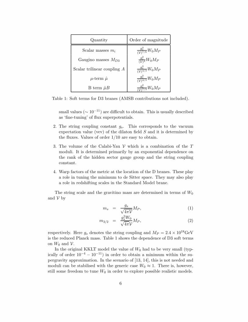
Table 1: Soft terms for D3 branes (AMSB contributions not included).

small values (∼ 10−11) are difficult to obtain. This is usually describedas ‘fine-tuning’ of flux superpotentials.

2. The string coupling constant gs. This corresponds to the vacuumexpectation value (vev) of the dilaton field S and it is determined bythe fluxes. Values of order 1/10 are easy to obtain.

3. The volume of the Calabi-Yau V which is a combination of the Tmoduli. It is determined primarily by an exponential dependence onthe rank of the hidden sector gauge group and the string couplingconstant.

4. Warp factors of the metric at the location of the D branes. These playa role in tuning the minimum to de Sitter space. They may also playa role in redshifting scales in the Standard Model brane.

The string scale and the gravitino mass are determined in terms of W0

and V by

ms =gs√4πV

MP , (1)

m3/2 =g2sW0√4πV

MP , (2)

respectively. Here gs denotes the string coupling and MP = 2.4 × 1018GeVis the reduced Planck mass. Table 1 shows the dependence of D3 soft termson W0 and V.

In the original KKLT model the value of W0 had to be very small (typ-ically of order 10−4 − 10−11) in order to obtain a minimum within the su-pergravity approximation. In the scenario of [13, 14], this is not needed andmoduli can be stabilised with the generic case W0 ≈ 1. There is, however,still some freedom to tune W0 in order to explore possible realistic models.

6

String scale ms complex structure, τs τb (lightest bulk modulus)

103GeV 1.5 × 10−11 2.2 × 10−25

105GeV 1.5 × 10−7 2.2 × 10−19

107GeV 1.5 × 10−4 2.2 × 10−13

109GeV 15 2.2 × 10−7

1011GeV 1.5 × 105 0.22

1013GeV 1.5 × 109 2.2 × 105

1015GeV 1.5 × 1013 2.2 × 1011

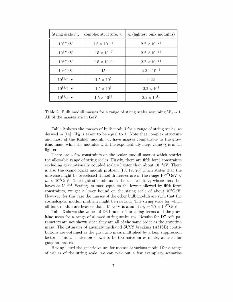
Table 2: Bulk moduli masses for a range of string scales assuming W0 ∼ 1.All of the masses are in GeV.

Table 2 shows the masses of bulk moduli for a range of string scales, asderived in [14]. W0 is taken to be equal to 1. Note that complex structureand most of the Kahler moduli, τs, have masses comparable to the grav-itino mass, while the modulus with the exponentially large value τb is muchlighter.

There are a few constraints on the scalar moduli masses which restrictthe allowable range of string scales. Firstly, there are fifth force constraintsexcluding gravitationally coupled scalars lighter than about 10−4eV. Thereis also the cosmological moduli problem [18, 19, 20] which states that theuniverse might be overclosed if moduli masses are in the range 10−7GeV <m < 104GeV. The lightest modulus in the scenario is τb whose mass be-haves as V−3/2. Setting its mass equal to the lowest allowed by fifth forceconstraints, we get a lower bound on the string scale of about 108GeV.However, for this case the masses of the other bulk moduli are such that thecosmological moduli problem might be relevant. The string scale for whichall bulk moduli are heavier than 104 GeV is around ms = 7.7 × 1012GeV.

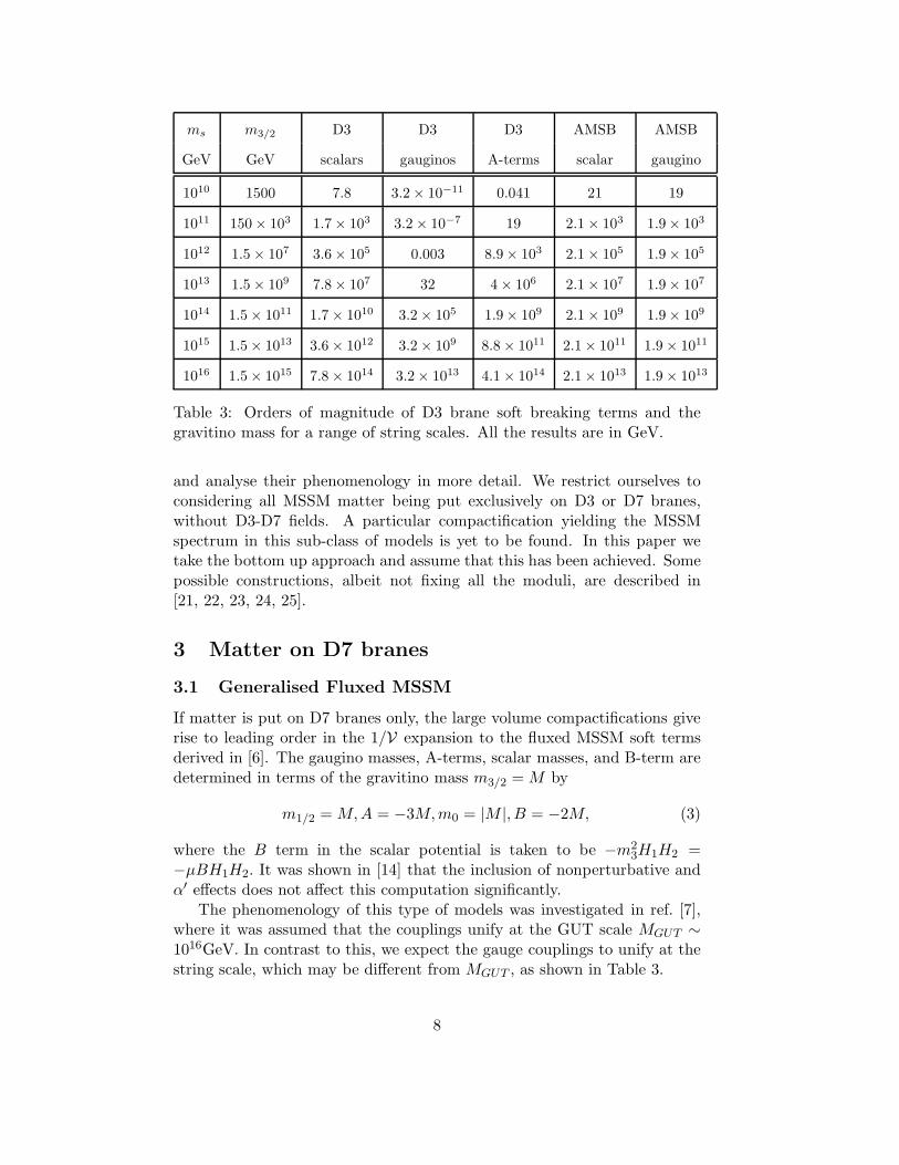
Table 3 shows the values of D3 brane soft breaking terms and the grav-itino mass for a range of allowed string scales ms. Results for D7 soft pa-rameters are not shown since they are all of the same order as the gravitinomass. The estimates of anomaly mediated SUSY breaking (AMSB) contri-butions are obtained as the gravitino mass multiplied by a loop suppressionfactor. This will later be shown to be too naive an estimate, at least forgaugino masses.

Having listed the generic values for masses of various moduli for a rangeof values of the string scale, we can pick out a few exemplary scenarios

7

ms m3/2 D3 D3 D3 AMSB AMSB

GeV GeV scalars gauginos A-terms scalar gaugino

1010 1500 7.8 3.2 × 10−11 0.041 21 19

1011 150 × 103 1.7 × 103 3.2 × 10−7 19 2.1 × 103 1.9 × 103

1012 1.5 × 107 3.6 × 105 0.003 8.9 × 103 2.1 × 105 1.9 × 105

1013 1.5 × 109 7.8 × 107 32 4 × 106 2.1 × 107 1.9 × 107

1014 1.5 × 1011 1.7 × 1010 3.2 × 105 1.9 × 109 2.1 × 109 1.9 × 109

1015 1.5 × 1013 3.6 × 1012 3.2 × 109 8.8 × 1011 2.1 × 1011 1.9 × 1011

1016 1.5 × 1015 7.8 × 1014 3.2 × 1013 4.1 × 1014 2.1 × 1013 1.9 × 1013

Table 3: Orders of magnitude of D3 brane soft breaking terms and thegravitino mass for a range of string scales. All the results are in GeV.

and analyse their phenomenology in more detail. We restrict ourselves toconsidering all MSSM matter being put exclusively on D3 or D7 branes,without D3-D7 fields. A particular compactification yielding the MSSMspectrum in this sub-class of models is yet to be found. In this paper wetake the bottom up approach and assume that this has been achieved. Somepossible constructions, albeit not fixing all the moduli, are described in[21, 22, 23, 24, 25].

3 Matter on D7 branes

3.1 Generalised Fluxed MSSM

If matter is put on D7 branes only, the large volume compactifications giverise to leading order in the 1/V expansion to the fluxed MSSM soft termsderived in [6]. The gaugino masses, A-terms, scalar masses, and B-term aredetermined in terms of the gravitino mass m3/2 = M by

m1/2 = M,A = −3M,m0 = |M |, B = −2M, (3)

where the B term in the scalar potential is taken to be −m23H1H2 =

−µBH1H2. It was shown in [14] that the inclusion of nonperturbative andα′ effects does not affect this computation significantly.

The phenomenology of this type of models was investigated in ref. [7],where it was assumed that the couplings unify at the GUT scale MGUT ∼1016GeV. In contrast to this, we expect the gauge couplings to unify at thestring scale, which may be different from MGUT , as shown in Table 3.

8

The large volume models impose a relationship between the gravitinomass M and the string scale ms. The string scale required for obtainingTeV size scalar masses, without any fine tuning in W0, is of the order 109 −1010GeV. However, it is well known that with the MSSM spectrum alone,the gauge couplings unify at approximately 1016GeV. In order to obtaingauge unification at a lowered scale, extra matter at a certain scale mustexist to modify the running of the gauge couplings 2. We choose this scale tobe 1TeV in order to avoid introducing a new hierarchy. Since the vector-likerepresentation of the additional matter allows for explicit mass terms, theyare expected to be of the order of the string scale and must therefore belowered to 1TeV by some mechanism. We will also assume that the Yukawacouplings of the extra matter to MSSM matter are negligible. To find outwhat extra matter needs to be added in order to achieve gauge unification,we may use the 1-loop RGEs for the MSSM including extra matter, foundin the Appendix of [26]. The relevant equations are

16π2 dg1

dt= g3

1

(

33

5+

nQ

5+

8nU

5+

2nD

5+

nS

10+

3

5n2 +

6

5nE

)

(4)

16π2 dg2

dt= g3

2 (1 + 3nQ + n2) (5)

16π2 dg3

dt= g3

3 (−3 + 2nQ + nU + nD + nS) . (6)

Here g1, g2, g3 are the gauge couplings for U(1), SU(2) and SU(3), respec-tively (g1 being GUT normalised), while t = ln µ with µ the DR renormal-isation scale. n2 is the number of additional vector-like lepton superfielddoublets L + L and nE the number of right handed lepton singlets E + E.nQ, nU , nD, nS are the numbers of Q + Q, U + U ,D + D and exotic “sex-tons” S which are colour triplets, electroweak singlets and have Y = 1/6.It is straightforward to see that lowering the string scale is easily achievedby using nonzero values only for n2, nE . A one loop analysis shows thatthe choice n2 = 4, nE = 6 unifies the couplings at approximately 1.2 × 109

GeV. To study the renormalisation group behaviour, we use SoftSUSY1.9

[27] modified so that RGEs with extra matter are used above the scale of1TeV. A 1-loop analysis is performed, giving a sufficient level of accuracyfor our needs. The values used for Standard Model input parameters arethe current central values: mt = 172.7GeV [28], mb(mb)

MS = 4.25GeV,

αs(MZ) = 0.1187, α−1(MZ)MS = 127.918, MZ = 91.1187GeV [29].For ms ∼ 109GeV, the RGE analysis results in the stop being the LSP.

This did not occur in the scenario with GUT scale unification. The reasonis that the scalar masses do not evolve sufficiently for a lowered string scale.

2For certain types of branes at singularities, gauge unification is not necessary. Simi-

larly this is true of models with intersecting or magnetised D-branes. We will investigate

this possibility later in the text.

9

0

100

200

300

400

500

600

102

104

106

108

1010

1012

1014

1016

1018

GeV

GeV

mtχ0

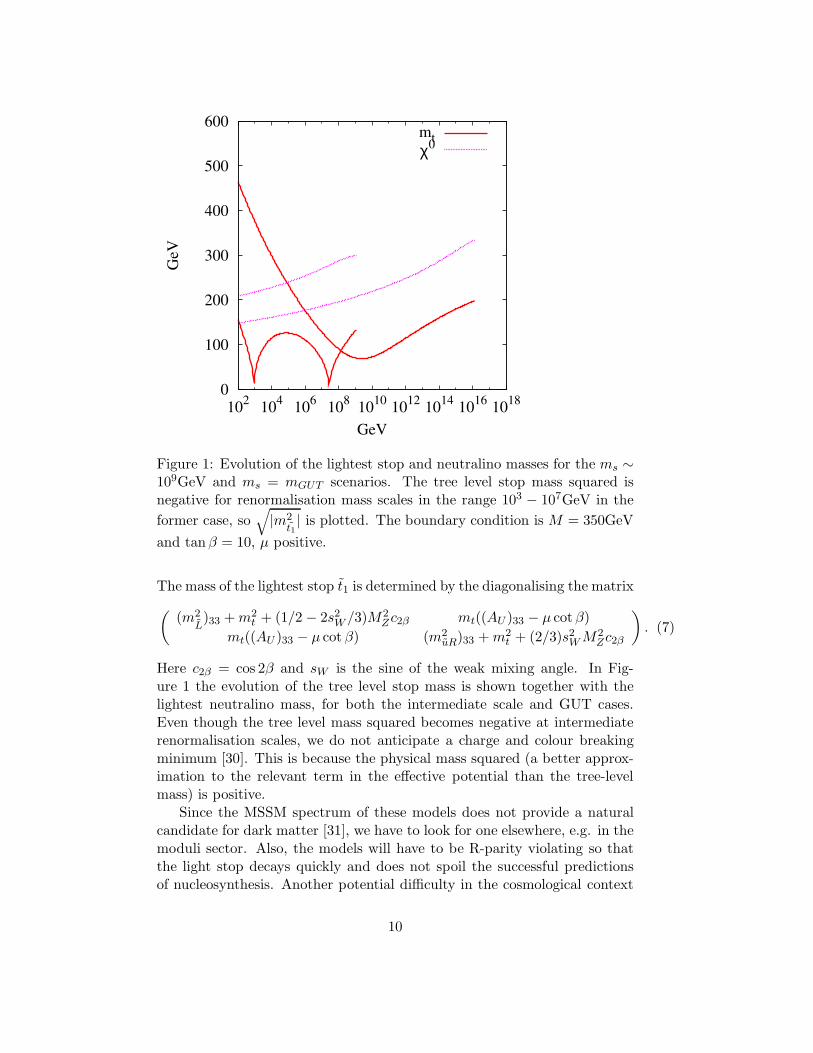
Figure 1: Evolution of the lightest stop and neutralino masses for the ms ∼109GeV and ms = mGUT scenarios. The tree level stop mass squared isnegative for renormalisation mass scales in the range 103 − 107GeV in the

former case, so√

|m2t1| is plotted. The boundary condition is M = 350GeV

and tan β = 10, µ positive.

The mass of the lightest stop t1 is determined by the diagonalising the matrix

(

(m2L)33 + m2

t + (1/2 − 2s2W /3)M2

Zc2β mt((AU )33 − µ cot β)

mt((AU )33 − µ cot β) (m2uR)33 + m2

t + (2/3)s2W M2

Zc2β

)

. (7)

Here c2β = cos 2β and sW is the sine of the weak mixing angle. In Fig-ure 1 the evolution of the tree level stop mass is shown together with thelightest neutralino mass, for both the intermediate scale and GUT cases.Even though the tree level mass squared becomes negative at intermediaterenormalisation scales, we do not anticipate a charge and colour breakingminimum [30]. This is because the physical mass squared (a better approx-imation to the relevant term in the effective potential than the tree-levelmass) is positive.

Since the MSSM spectrum of these models does not provide a naturalcandidate for dark matter [31], we have to look for one elsewhere, e.g. in themoduli sector. Also, the models will have to be R-parity violating so thatthe light stop decays quickly and does not spoil the successful predictionsof nucleosynthesis. Another potential difficulty in the cosmological context

10

could be posed by the light bulk moduli for the string scale of order 109GeV,as pointed out in Section 2.

The models can still be subjected to other experimental constraints, suchas the ones coming from precision measurements of the b → sγ branchingratio and the anomalous magnetic moment of the muon.

The most recent average measurement of the b → sγ branching ratio maybe obtained from [32] and is (3.39±0.30)×10−4 . The theoretical uncertaintyin this result is [33] 0.30 × 10−4; adding the two errors in quadrature, weobtain the 1σ bound, BR(b → sγ) = (3.4 ± 0.4) × 10−4.

We also impose limits on the new physics contribution to aµ = (gµ−2)/2.The experimental value of aµ is (11659208 ± 6) × 10−10 [34]. The StandardModel computation yields [35, 36] (11659189 ± 6) × 10−10 for the samequantity. This results in the 1σ bound on the non-SM contribution to aµ,δaµ = (19± 9)× 1010. It is important to note that δaµ usually has the samesign as µ, so µ > 0 is preferred by experiment.

We also impose bounds on the Higgs mass obtained by the LEP2 col-laborations [37]. The lower bound is 114.4 GeV at the 95% CL. The errorin theoretical predictions is estimated to 3GeV so we require mh > 111GeVon the SoftSUSY1.9 prediction.

One can consider a simple modification of this scenario with a raisedstring scale, by allowing some fine tuning in W0. Namely, one can decreaseV while decreasing W0, hence increasing ms but also decreasing the amountof SUSY breaking. Let us consider the cases ms ∼ 1012GeV and ms ∼1014GeV 3. In the former case, to make the gauge couplings unify at thestring scale, we add n2 = 2, nE = 3. In the ms ∼ 1014GeV case, we needto add n2 = 1, nE = 1. Interestingly, already in the ms ∼ 1012GeV case,the LSP becomes a neutralino. We can then apply the hypothesis that theneutralino constitutes all of the cold dark matter relic density. The WMAP[38, 39] constraint on the relic density of dark matter particles (at the 3σlevel) is

0.084 < Ωh2 < 0.138. (8)

However, the B = −2M condition cannot be satisfied for any valuesof ms,M with µ > 0 and can only be satisfied for µ < 0 for string scales1014GeV and above. To see this, one notes that the EWSB conditions

µ2 =−m2

H1tan2 β + m2

H1

tan2 β − 1− 1

2M2

Z , (9)

µB =1

2sin 2β(m2

H1+ m2

H2+ 2µ2) (10)

determine the values of B and µ at the scale MSUSY =√

mt1mt2

in termsof tan β and the soft breaking masses mH1

,mH2. One then needs to evolve

3It should be noted that lifting the string scale does not remove the cosmological

problems associated with light bulk moduli, since masses of some of these are proportional

to W0.

11

0

0.2

0.4

0.6

0.8

1

1.2

1.4

0 5 10 15 20 25 30 35 40

-B/(

2M

)

tan β

m=109, M=350GeV

m=109, M=1300GeV

m=1012

. M=350GeVm=10

12, M=1300GeV

m=1014

. M=350GeVm=10

14, M=1300GeV

0

0.2

0.4

0.6

0.8

1

1.2

1.4

0 5 10 15 20 25 30 35 40

-B/(

2M

)

tan β

m=109, M=350GeV

m=109, M=1300GeV

m=1012

. M=350GeVm=10

12, M=1300GeV

m=1014

. M=350GeVm=10

14, M=1300GeV

(a) (b)

Figure 2: Ratio B(ms)/2M for (a) µ > 0 and (b) µ < 0, M = 350GeV andM = 1300GeV.

back to the string scale to check whether the condition B = −2M can besatisfied.

The dependence of the ratio |B|/(2M) on tan β is displayed in Figure 2,for various choices of string scale. Solutions to B = −2M exist only for thelow tan β region and µ < 0. However, it can be verified that in this region,the Higgs is too light compared to the LEP2 bound.

Therefore we will neglect for the time being the boundary condition B =−2M , assuming that the values for the µ and B-terms required for correctelectroweak symmetry breaking (EWSB) are generated by some unknownmechanism.

There are then two free parameters, the mass scale M and tan β. The b →sγ branching ratio, δaµ and Ωh2 are computed using the micrOmegas1.3

package [40] interfaced with SoftSUSY1.9 via the SUSY Les Houches Accord[41]. The results are plotted in Figure 3 for ms ∼ 109GeV and in Figure 4for ms ∼ 1012GeV. Although the dark matter relic density computation issensitive to the details of the low energy spectrum, the allowed region in theM−tan β plane should not shift significantly when two-loop RGE equationsare used instead of one-loop ones. Note that for tan β greater than around40 one cannot obtain correct EWSB and those values are not included inthe graphs. Because the LSP is the stop for ms ∼ 109GeV, we do not plotΩh2 in Figure 3.

MSSM spectra for a few sample points in the parameter space for whichboth the δaµ and BR(b → sγ) constraints are satisfied are shown in Table 4.

12

5

10

15

20

25

30

35

40

45

200 400 600 800 1000 1200

tan

β

M/GeV

2.5x10-4

111 GeV

2x10-10

allowedtachyons

A

δµb->sγ

mh

5

10

15

20

25

30

35

40

45

200 400 600 800 1000 1200

tan

β

M/GeV

4.8x10-4

111 GeV

-6x10-10

allowed

tachyons

B

δµb->sγ

mh

(a) (b)

Figure 3: Contour plots of δaµ and BR(b → sγ) on tan β and M for (a)µ > 0 and (b) µ < 0 and ms ∼ 109 GeV. 2σ bounds are used for µ > 0 while3σ ones are used for µ < 0.

5

10

15

20

25

30

35

40

45

200 400 600 800 1000 1200

tan

β

M/GeV

36x10-10

2.0x10-10

2.5x10-4

111 GeV

allowed

C

δµb->sγ

mhΩ h2

5

10

15

20

25

30

35

40

45

200 400 600 800 1000 1200

tan

β

M/GeV

4.8x10-4

111 GeV

-6x10-10

allowed

D

δµb->sγ

mhΩ h2

(a) (b)

Figure 4: Contour plots of δaµ, BR(b → sγ) and Ωh2 on tan β and M for(a) µ > 0 and (b) µ < 0 and ms ∼ 1012 GeV. 2σ bounds are used for µ > 0while 3σ ones are used for µ < 0.

13

The points chosen are denoted by A,B in Figure 3 and C,D in Figure 4. PointC satisfies all the constraints, including the χ0

1 cold dark matter hypothesis.The other points satisfy the BR(b → sγ) and (g − 2)µ constraints. In thems ∼ 1012GeV, µ < 0 case, it is not possible to satisfy the dark matterconstraint.

As mentioned before, it is also possible to construct models where gaugeunfication does not take place at the string scale. We investigate that possi-bility for completeness, using the standard MSSM RGEs without any extramatter. In this case, two loop RGEs are used rather than one loop RGEs.The results, however, turn out not to differ significantly from the unificationat ms scenario.

4 Matter on D3 branes

Let us now investigate the semi-realistic scenarios that can be constructedassuming the Standard Model lives on a set of D3 branes. For this we haveto consider the spectrum in Table 3. Notice that there is a hierarchy betweenthe scalar and the gaugino masses. The difference between the two massesdecreases when the string scale is increased. At the GUT scale they tendto be of the same size but apparently too heavy. For any other scale thescalars are much heavier than the gauginos. At an intermediate string scalethe scalar masses are of order 1 TeV but the gauginos are too light. Atfirst sight we might conclude that anomaly mediation contribution to thegaugino masses would be dominant but the no-scale nature of our models issuch that this contribution is also negligible.

Loop corrections are not large enough to lift the gaugino masses to re-alistic values. Only for A terms of order ∼ 107GeV loop corrections inducegaugino masses of order TeV but at that scale scalar masses are very heavy(∼ 107GeV). We then would have to argue that fine-tuning similar to splitsupersymmetry is at work to keep the Higgs light.

A second alternative is to consider the case in which the scalar andgaugino masses are of the same order, which in Table 3 corresponds to theGUT scale. Again, the value of W0 can be fine tuned to lower the effectivemasses of scalars and gauginos to the TeV range. We will consider next eachof these two scenarios.

4.1 Intermediate Scale Split SUSY

We choose the string scale to be ∼ 1013GeV, with the scalar masses of order107GeV. One might worry that the gauginos will be extremely heavy as welldue to the AMSB contribution. However, it was shown in [42] that in no-scale type models the AMSB contribution to the gaugino mass is vanishing(see the Appendix).

14

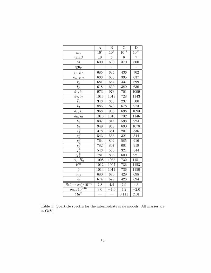
A B C D

ms 109 109 1012 1012

tan β 10 5 6 7

M 600 600 370 600

sgnµ + - + -

eL, µL 685 684 436 702

eR, µR 633 633 395 637

τL 681 684 437 699

τR 618 630 389 630

u1, c1 973 973 701 1099

u2, c2 1013 1013 728 1143

t1 343 385 237 500

t2 885 873 678 973

d1, s1 968 968 698 1093

d2, s2 1016 1016 732 1146

b1 807 814 593 924

b2 949 958 690 1078

χ01 378 381 201 336

χ02 543 556 321 544

χ03 764 802 585 916

χ04 782 807 601 919

χ±1 543 556 321 544

χ±2 781 808 600 921

A0,H0 1008 1065 732 1151

H± 1012 1067 736 1153

g 1014 1014 736 1150

ν1,2 680 680 429 698

ν3 674 679 428 694

B(b → sγ)/10−4 2.8 4.4 2.9 4.3

δaµ/10−10 3.0 −1.6 4.2 −2.0

Ωh2 — — 0.111 2.01

Table 4: Sparticle spectra for the intermediate scale models. All masses arein GeV.

15

There are two kinds of corrections to this result in our models - firstly,we include perturbative α′ corrections in the Kahler potential, and secondly,we include nonperturbative contributions to the superpotential W. At treelevel, the gaugino masses are set by the size of FS , which is induced bynonzero mixing between the dilaton and Kahler moduli once α′ correctionsare included. However, FS is proportional to 1/V2 and is very small forlarge volume. As seen above, the one loop anomaly-induced contributionalso vanishes in the no-scale approximation.

In the two Kahler modulus model investigated in [14], we have ∂sK ∼1V

and ∂bK ∼ 1V2/3

with s, b denoting the small and large Kahler moduli,

respectively. The nonperturbative contributions to the F-terms are Fnps ∼ 1

V

and Fnpb ∼ 1

V4/3. Therefore, the contributions KiF

inp to the gaugino mass

in formula (23) in the Appendix scale like 1/V2. Similarly, the contributionto gaugino masses from FS is of the same form. Therefore the anomalycontribution is not as large as would follow from the naive estimate basedon just including the superconformal anomaly contribution proportional tom3/2.

Hence we arrive at a scenario with the string scale at around 1013GeV,the scalar masses at m ∼ 107GeV and gaugino masses approximately van-ishing at the string scale. The first question to be considered is whether it ispossible to generate gaugino masses sufficiently large to pass experimentallower bounds through RG evolution to lower scales. To answer this, onemust consider the two-loop MSSM RGEs for gaugino masses (as found in[43]):

d

dtMa =

2g2a

16π2baMa+ (11)

2g2a

(16π2)2

∑

b

Babg2b (Ma + Mb) +

∑

α=u,d,e

Cαa (tr(Y α†hα) − Matr(Y

α†

Y α))

.

The SUSY breaking trilinear scalar couplings hα (defined in terms of themore familiar A notation via hα

ij = AαijY

αij , Y α being the Yukawa couplings)

enter the two loop renormalisation; if they are large enough it might bepossible to generate sufficient gaugino masses in the running between thestring scale and the scalar mass scale.

We will have to assume that the Higgs mass squared is fine-tuned at thescalar mass scale to be negative and of order −m2

ew. Given this assumption,below scale m, the effective field theory spectrum is that of split super-symmetry [44, 45]: all the SM particles including one light Higgs doubletH, together with gauginos B, W , g and higgsinos Hu, Hd. The Lagrangianconsists of kinetic terms and

m2H†H − λ

2(H†H)2 −

(

Y uij qjuiǫH

∗ + Y dij qjdiH + Y e

ij ljeiH

16

+M3

2gAgA +

M2

2W aW a +

M1

2BB + µHT

u ǫHd

+H†

√2(guσaW a + g′uB)Hu +

HT ǫ√2

(−gdσaW a + g′dB)Hd + h.c.

)

, (12)

where σa are the Pauli matrices and ǫ = iσ2. Below the scale of the scaleof the scalar masses, we use the RGEs of split supersymmetry, listed in theAppendix of [45].

The simplest experimental constraint to impose is the one on the Higgsmass. The Higgs quartic coupling λ is matched at the scalar mass scale bythe formula

λ(m) =g2(m) + g′2(m)

4cos2 2β. (13)

g and g′ are the values of the SU(2) and U(1)Y gauge couplings, and therelation between the GUT normalised g1 and g′ is g1 =

√

5/3g′. Equation(13) can be obtained by matching the split SUSY Lagrangian (12) with theusual SUSY Lagrangian valid above the scalar mass m. It receives finitethreshold corrections of order A2/m2, but this is negligible in our models.The boundary conditions for gu,d, g

′u,d are similarly given at scale m in terms

of g, g′ and tan β. The values of g, g′ at the scale m are found by a simpleone-loop evolution from their experimentally determined values at MZ ; afterthat one evolves λ down to MZ using the split SUSY RGEs.

The renormalisation effects on λ are large and it is natural to obtaina Higgs significantly heavier than the LEP2 bound. The Higgs mass isestimated as mH =

√λv with v = 246.22GeV. mH ranges from ∼ 142

GeV to ∼ 163 GeV depending on the values of tan β, the top mass and thescalar masses m. The principal dependency is through the value of the topYukawa, i.e. the top mass. The tree level formula for the Yukawa coupling ismpole

t

√2 = yt(mt)v(mt), giving yt = 0.99 for mt = 172.7 GeV. The dominant

one loop corrections to this are [47]

mpolet

√2 = yt(mt)v(mt)

(

1 +g23(mt)

3π2− y2

t (mt)

8π2

)

, (14)

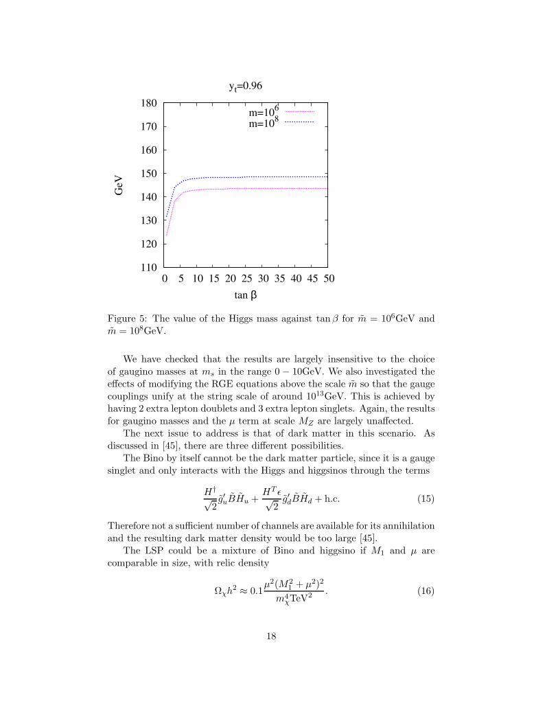
giving yt(mt) = 0.96. We use the 1-loop corrected value for greater accuracy.As can be seen in Figure 5, the Higgs mass is essentially independent of tan βfor large values of tan β.

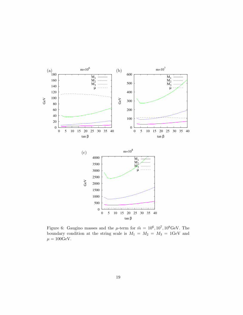
Next we study the RGE evolution of gaugino masses and the µ-term. Weassume that the gaugino masses at the high scale are close to 0GeV and thatthe magnitude of the µ-term is tuned to 100GeV. The A-terms are taken tobe negative and between 104 and 107 GeV in magnitude. With these initialconditions at the string scale ms we evolve down to the scalar mass scalem. The results for gaugino masses and the µ-term at the scale of MZ areshown in Figure 6. The salient features are a heavy gluino, a slight changein the µ-term, a small increase in M1, and a moderate one in M2.

17

110

120

130

140

150

160

170

180

0 5 10 15 20 25 30 35 40 45 50

GeV

tan β

yt=0.96

m=106

m=108

Figure 5: The value of the Higgs mass against tan β for m = 106GeV andm = 108GeV.

We have checked that the results are largely insensitive to the choiceof gaugino masses at ms in the range 0 − 10GeV. We also investigated theeffects of modifying the RGE equations above the scale m so that the gaugecouplings unify at the string scale of around 1013GeV. This is achieved byhaving 2 extra lepton doublets and 3 extra lepton singlets. Again, the resultsfor gaugino masses and the µ term at scale MZ are largely unaffected.

The next issue to address is that of dark matter in this scenario. Asdiscussed in [45], there are three different possibilities.

The Bino by itself cannot be the dark matter particle, since it is a gaugesinglet and only interacts with the Higgs and higgsinos through the terms

H†

√2g′uBHu +

HT ǫ√2

g′dBHd + h.c. (15)

Therefore not a sufficient number of channels are available for its annihilationand the resulting dark matter density would be too large [45].

The LSP could be a mixture of Bino and higgsino if M1 and µ arecomparable in size, with relic density

Ωχh2 ≈ 0.1µ2(M2

1 + µ2)2

m4χTeV2 . (16)

18

0

500

1000

1500

2000

2500

3000

3500

4000

0 5 10 15 20 25 30 35 40

GeV

tan β

m=108

M1M2M3

µ

0

20

40

60

80

100

120

140

160

180

0 5 10 15 20 25 30 35 40

GeV

tan β

m=106

M1M2M3

µ

0

100

200

300

400

500

600

0 5 10 15 20 25 30 35 40

GeV

tan β

m=107

M1M2M3

µ

(c)

(a) (b)

Figure 6: Gaugino masses and the µ-term for m = 106, 107, 108GeV. Theboundary condition at the string scale is M1 = M2 = M3 = 1GeV andµ = 100GeV.

19

Particle Mass

χ01 123

χ02 204

χ03 240

χ04 407

χ+1 212

χ+2 383

g 1033

Ωh2 0.11

Table 5: Supersymmetric particle spectrum for m = 107GeV, µ = 200GeVand tan β = 22.

We consider the m = 107GeV scenario, with µ = 200GeV at the stringscale. The relic density is computed using formula (16) and its dependenceon tan β is shown in Figure 7. Also included is the graph of the relic densityfor m = 108GeV and µ = 500GeV at the string scale. It is clear thatwith appropriately chosen values of µ and tan β it is possible to obtainan acceptable dark matter relic density. The particle spectrum for m =107GeV, µ = 200GeV and tan β = 22, satisfying the dark matter hypothesis,is shown in Table 5.

The second case is that of a heavy higgsino being the LSP. In this casethe relic abundance is

ΩHh2 = 0.09( µ

TeV

)2. (17)

Scenarios with m slightly above 108GeV can realise this possibility,since then the Bino has mass above 700GeV. With a µ-term chosen to be1 − 1.2TeV at the string scale ms, it is possible to obtain the correct relicabundance. For example, with A = −3 × 106GeV and tan β = 40 we have(at scale MZ) M1 ∼ 2200GeV, M2 ∼ 5600GeV, M3 ∼ 12000GeV whereasµ = 1006GeV.

The last possibility is that of a Wino LSP and relic abundance

ΩW h2 = 0.02

(

M2

TeV

)2

. (18)

However, this cannot be realised in our scenarios, since the Wino is alwaysheavier than the Bino.

4.2 Stringy mSUGRA

We note that the string scale is independent of the flux superpotential pa-rameter W0, whereas all the soft terms are directly proportional to it. There-fore we can take ms ∼ 1016GeV, put all the matter on D3 branes and lower

20

0

0.2

0.4

0.6

0.8

1

0 5 10 15 20 25 30 35 40 45

Ω h

2

tan β

allowed

m=107, µ=200

m=108, µ=500

Figure 7: The dark matter relic density Ωh2 in the heavy scalar scenario,for m = 107GeV, µ = 200GeV and m = 108GeV, µ = 500GeV.

the value of W0 to obtain realistic values for the scalar masses and othersoft parameters. Note that the gravitino mass will also be lowered in thisprocess, and its size will be roughly just one order of magnitude above thescalar masses. We must be careful for a number of reasons, since loweringW0 means lowering the magnitude of supersymmetry breaking in the non-SUSY AdS minimum of [14]. Therefore the D-term contribution to SUSYbreaking might become significant compared to the F-term contributions.However, this is not the case since both D and F-terms are proportional tothe value of W0.

Therefore, we have two parameters to control - V and W0. IncreasingV decreases the string scale, while decreasing W0 decreases the soft termsonly (since the amount of supersymmetry breaking is reduced). However,the only reasonable scenarios with scalar masses of O(1TeV) will arise fromthe scenario with string scale 1016GeV and appropriately reduced W0. Thestring scale cannot be reduced any further, since that would entail increasingV significantly and the ratio of gaugino to scalar masses would become verysmall, leading back to the split SUSY scenario.

21

5 Other possibilities

One could also consider D3 or D7 branes in a warped region, so that thewarp factor reduces the scalar masses to a small value. This however alsoreduces the value of the string scale to a smaller value. The resulting smallgap between the scalar mass scale and the string scale makes it difficult toachieve unification at the string scale - one needs a large amount of extramatter. For example, if the string scale is lowered to 106 GeV, one needsat least 14 new multiplets, and with the string scale at 104GeV, one needs51. The construction of string models in which this type of scenarios can berealised is open.

6 Conclusions

We have presented three distinctive scenarios of low-energy supersymmetrybreaking which were derived from string compactifications. It is very ap-pealing to be able go such a long way - from a string theory compactificationwith fluxes to computing the spectrum at low energy of specific models. Itis also illustrative to see how difficult it is to obtain fully realistic scenariosgiven the many cosmological and phenomenological constraints.

The three scenarios we studied have several interesting properties andrepresent a progress in the right direction to close the gap between stringtheory and low-energy physics. In particular the detailed spectrum of su-persymmetric particles was obtained at low-energies for representative ex-amples.

Each of the scenarios has potential problems which illustrate the difficul-ties that can be expected in general. The generalised fluxed MSSM scenario,despite its interesting features, has to face the cosmological moduli problemwhich appears at every value of the string scale, as mentioned in the text.We would have to rely on a solution of this problem in order to considerthis scenario to be fully realistic. Notice that this potential problem couldnot have been envisioned in the original discussion of soft supersymmetrybreaking induced by fluxes since there was no mechanism to fix the Kahlerstructure moduli. Also, for scales lower than 1012GeV the stop is the LSPinstead of a neutralino. Barring these problems we found that the parameterspace is greatly reduced by the standard phenomenological constraints. Thecase µ > 0 is not compatible with the boundary condition for the B term,while for µ < 0,ms < 1016GeV only low tan β solutions exist and the Higgsmass is below the LEP2 bound. This problem may be alleviated by relaxingthe B term boundary condition, e.g. by considering the Higgs coming fromD3-D7 strings. Our lack of control of the Kahler potential for these fieldsdoes not allow us to make a concrete statement about this possibility.

The intermediate scale split supersymmetry scenario needs the usual fine

22

tuning in order to keep the Higgs light. Again the D3-D7 particles couldalleviate this problem if their masses were under control. Furthermore,despite sharing with the split supersymmetry scenario the property that thescalars are hierarchically heavier than the gauginos, it has to be pointed outthat in our scenario the string scale is intermediate and therefore we do notexpect the standard MSSM gauge coupling unification to work.

The stringy mSUGRA scenario requires a tuning of the flux superpoten-tial in order to achieve a GUT string scale. This tuning however may beargued to be less severe than the tuning of the split supersymmetry thatneeds to be made at the spectrum level, although both rely on the existenceof many flux vacua. Notice that in the stringy mSUGRA scenario, with-out knowing any relationship among the relative coefficients, we can onlyestimate the order of magnitude of the soft breaking terms.

It is fair to say also that each of the phenomenological constraints wehave used may be relaxed and the parameter space of realistic models canbe substantially enhanced. For example, non-universal flavour structure inthe soft SUSY breaking terms can cancel the supersymmetric contributionto BR(b → sγ). Also, evidence for a non-Standard Model component of(g − 2)µ is controversial and may turn out to not be relevant. Similarly,dark matter could all reside in the hidden sector and the LSP could beunstable.

It is interesting to compare our results with the phenomenology of KKLT-type scenarios. The essential difference is that the large volume minima wefound are non-supersymmetric even before the lifting term is added. InKKLT scenarios, supersymmetry is restored after fixing the Kahler moduli,so it is precisely the anti D3 brane term which is responsible for supersym-metry breaking. Of course, the uplift gives non-zero values to F-terms aswell, but these will be parametrised in terms of the uplift potential. In factit turns out [8, 9] that they are significantly suppressed with respect to theno-scale model values. This implies that, for example, the moduli mediatedcontribution to the D7 scalar masses is suppressed with respect to m3/2 andwill generically compete with the AMSB contribution. The same is true forgaugino masses, where it turns out that it is possible to obtain a ‘mirageunification’ at the intermediate or even TeV scale by combining the two con-tributions [10, 11, 12]. There were no realistic scenarios for D3 soft termsin that scenario.

Finally, it is worth pointing out that what we have analysed here aregeneral scenarios assuming that the Standard Model is on D3 or D7 branes.In order to be more concrete it would be desirable to carry out this kind ofanalysis on explicit D-brane models, taking into account potential matterand gauge fields beyond the MSSM, etc. There are clearly many things tobe done in this direction. Explicit model building may become more focusedafter data from the Large Hadron Collider (LHC) arrives.

23

Acknowledgments

We would like to thank Cliff Burgess, Joseph Conlon and Luis Ibanez foruseful conversations. We also thank Gordon Kane and Piyush Kumar forcomments on an earlier version of the paper. This research is partiallyfunded by PPARC. FQ is also funded by a Royal Society Wolfson award.KS is grateful to Trinity College, Cambridge for financial support.

A Appendix: Gaugino Masses in No-Scale Models

Let us consider the general formula for the gaugino mass in models withboth moduli and anomaly mediated SUSY breaking, as derived in [42]:

mG = − g2

16π2

(

(3TG − TR)m3/2 + (TG − TR)KiFi +

2TR

dR(log det K|′′R),iF

i

)

(19)Here TG is the Dynkin index for the adjoint representation, 3TG −TR is theone-loop gauge beta function coefficient and TR is the Dynkin index associ-ated with the representation R of dimension dR, equal to 1/2 for the SU(N)fundamental; a sum over all the matter representations R is understood ineach term with the R subindex. K is the Kahler potential, K ′′|R its secondderivatives with respect to matter fields projected onto the correspondingrepresentation of G, and the F-terms are defined as4

F i = −eK/2Ki DjW, (20)

with W the superpotential. The first term in equation (19) is the usualsuper-Weyl anomaly induced term present in any supergravity theory. Thesecond and third terms arise from Kahler and sigma-model anomalies.

For simplicity let us consider the case of a single Kahler modulus model.Let us assume that the Kahler potential is of the no-scale form,

K = −3 log

(

T + T ∗ − 1

3φφ∗

)

(21)

where φ is the matter field. Taking derivatives with respect to matter fields,one gets the result for a particular representation R

1

dRlog detK|′′R =

1

3K, (22)

assuming that the vevs of visible matter vanish. Hence from formula (19)we get

mG = − g2

16π2

(

(3TG − TR)m3/2 + (TG − TR)KiFi +

2

3TRKiF

i

)

(23)

4The minus sign is inserted to make the definition agree with the global supersymmetry

one in the limit MP → ∞.

24

= − g2

48π2(3TG − TR)(3m3/2 + KiF

i). (24)

In no-scale models SUSY breaking corresponds to nonzero values of theauxiliary field corresponding to T. The gravitino mass is equal to

m3/2 = eK/2W. (25)

Also

F T = −eK/2KT T DT W = −eK/2 (T + T ∗)2

3(∂T K)W = eK/2(T + T ∗)W.

(26)assuming that T is absent from the superpotential. Therefore we have

KT F T + 3m3/2 = −3eK/2W + 3eK/2W = 0. (27)

It can easily be checked that this result generalises to the n-Kahler moduluscase, due to the no-scale property Ki∂iK∂K = 3 with i, j ranging over allKahler moduli. It follows from equation (23) that the AMSB contributionto gaugino masses is vanishing.

References

[1] D. J. H. Chung, L. L. Everett, G. L. Kane, S. F. King, J. D. Lykken andL. T. Wang, “The soft supersymmetry-breaking Lagrangian: Theoryand applications,” Phys. Rept. 407, 1 (2005) [arXiv:hep-ph/0312378].

[2] B. C. Allanach et al., “The Snowmass points and slopes: Bench-marks for SUSY searches,” in Proc. of the APS/DPF/DPB Sum-mer Study on the Future of Particle Physics (Snowmass 2001) ed.N. Graf, Eur. Phys. J. C 25, 113 (2002) [eConf C010630, P125 (2001)][arXiv:hep-ph/0202233].

[3] M. Battaglia et al., “Proposed post-LEP benchmarks for supersymme-try,” Eur. Phys. J. C 22, 535 (2001) [arXiv:hep-ph/0106204].

[4] A. Brignole, L. E. Ibanez and C. Munoz, “Soft supersymmetry-breaking terms from supergravity and superstring models,”arXiv:hep-ph/9707209.

[5] S. Kachru, R. Kallosh, A. Linde and S. P. Trivedi, “De Sitter vacua instring theory,” Phys. Rev. D 68, 046005 (2003) [arXiv:hep-th/0301240].

[6] M. Grana, “MSSM parameters from supergravity backgrounds,” Phys.Rev. D 67, 066006 (2003) [arXiv:hep-th/0209200];

25

P. G. Camara, L. E. Ibanez and A. M. Uranga, “Flux-inducedSUSY-breaking soft terms,” Nucl. Phys. B 689, 195 (2004)[arXiv:hep-th/0311241];

M. Grana, T. W. Grimm, H. Jockers and J. Louis, “Soft supersymmetrybreaking in Calabi-Yau orientifolds with D-branes and fluxes,” Nucl.Phys. B 690, 21 (2004) [arXiv:hep-th/0312232];

D. Lust, S. Reffert and S. Stieberger, “Flux-induced soft supersymme-try breaking in chiral type IIb orientifolds with D3/D7-branes,” Nucl.Phys. B 706, 3 (2005) [arXiv:hep-th/0406092];

P. G. Camara, L. E. Ibanez and A. M. Uranga, “Flux-induced SUSY-breaking soft terms on D7-D3 brane systems,” Nucl. Phys. B 708, 268(2005) [arXiv:hep-th/0408036].

A. Font and L. E. Ibanez, “SUSY-breaking soft terms in aMSSM magnetized D7-brane model,” JHEP 0503, 040 (2005)[arXiv:hep-th/0412150].

[7] B. C. Allanach, A. Brignole and L. E. Ibanez, “Phenomenology of afluxed MSSM,” JHEP 0505, 030 (2005) [arXiv:hep-ph/0502151].

[8] K. Choi, A. Falkowski, H. P. Nilles and M. Olechowski, “Soft supersym-metry breaking in KKLT flux compactification,” Nucl. Phys. B 718, 113(2005) [arXiv:hep-th/0503216].

[9] A. Falkowski, O. Lebedev and Y. Mambrini, “SUSY phenomenology ofKKLT flux compactifications,” arXiv:hep-ph/0507110.

[10] K. Choi, K. S. Jeong and K. i. Okumura, “Phenomenology of mixedmodulus-anomaly mediation in fluxed string compactifications andbrane models,” JHEP 0509, 039 (2005) [arXiv:hep-ph/0504037].

[11] M. Endo, M. Yamaguchi and K. Yoshioka, “A bottom-up approachto moduli dynamics in heavy gravitino scenario: Superpotential, softterms and sparticle mass spectrum,” Phys. Rev. D 72, 015004 (2005)[arXiv:hep-ph/0504036].

[12] O. Lebedev, H. P. Nilles and M. Ratz, “A note on fine-tuning in miragemediation,” arXiv:hep-ph/0511320.

[13] V. Balasubramanian, P. Berglund, J. P. Conlon and F. Quevedo, “Sys-tematics of moduli stabilisation in Calabi-Yau flux compactifications,”JHEP 0503, 007 (2005) [arXiv:hep-th/0502058].

[14] J. P. Conlon, F. Quevedo and K. Suruliz, “Large-volume flux compact-ifications: Moduli spectrum and D3/D7 soft JHEP 0508, 007 (2005)[arXiv:hep-th/0505076].

26

[15] L. E. Ibanez, “The fluxed MSSM,” Phys. Rev. D 71, 055005 (2005)[arXiv:hep-ph/0408064].

[16] C. P. Burgess, R. Kallosh and F. Quevedo, “de Sitter stringvacua from supersymmetric D-terms,” JHEP 0310 (2003) 056[arXiv:hep-th/0309187]; G. Villadoro and F. Zwirner, “de Sitter vacuavia consistent D-terms,” arXiv:hep-th/0508167.

[17] A. Saltman and E. Silverstein, “The scaling of the no-scale po-tential and de Sitter model building,” JHEP 0411 (2004) 066[arXiv:hep-th/0402135].

[18] T. Banks, D. B. Kaplan and A. E. Nelson, “Cosmological implicationsof dynamical supersymmetry breaking,” Phys. Rev. D 49, 779 (1994)[arXiv:hep-ph/9308292].

[19] B. de Carlos, J. A. Casas, F. Quevedo and E. Roulet, “Model in-dependent properties and cosmological implications of the dilatonand moduli sectors of 4-d strings,” Phys. Lett. B 318, 447 (1993)[arXiv:hep-ph/9308325].

[20] G. D. Coughlan, W. Fischler, E. W. Kolb, S. Raby and G. G. Ross,“Cosmological Problems For The Polonyi Potential,” Phys. Lett. B 131,59 (1983).

[21] G. Aldazabal, L. E. Ibanez, F. Quevedo and A. M. Uranga, “D-branesat singularities: A bottom-up approach to the string embedding ofthe standard model,” JHEP 0008, 002 (2000) [arXiv:hep-th/0005067];G. Aldazabal, L. E. Ibanez and F. Quevedo, “Standard-like models withbroken supersymmetry from type I string vacua,” JHEP 0001 (2000)031 [arXiv:hep-th/9909172]; “A D-brane alternative to the MSSM,”JHEP 0002 (2000) 015 [arXiv:hep-ph/0001083].

[22] J. F. G. Cascales, M. P. Garcia del Moral, F. Quevedo andA. M. Uranga, “Realistic D-brane models on warped throats: Fluxes,hierarchies and moduli stabilization,” JHEP 0402, 031 (2004)[arXiv:hep-th/0312051].

[23] D. Berenstein, V. Jejjala and R. G. Leigh, “The standard model on aD-brane,” Phys. Rev. Lett. 88, 071602 (2002) [arXiv:hep-ph/0105042].

[24] H. Verlinde and M. Wijnholt, “Building the standard model on a D3-brane,” arXiv:hep-th/0508089.

[25] J. F. G. Cascales, F. Saad and A. M. Uranga, “Holographic dual of thestandard model on the throat,” arXiv:hep-th/0503079.

27

[26] B. C. Allanach and S. F. King, “String unification, spaghetti di-agrams and infra-red fixed points,” Nucl. Phys. B 507, 91 (1997)[arXiv:hep-ph/9703293].

[27] B. C. Allanach, “SOFTSUSY: A C++ program for calculating su-persymmetric spectra,” Comput. Phys. Commun. 143, 305 (2002)[arXiv:hep-ph/0104145].

[28] [CDF Collaboration], “Combination of CDF and D0 results on the top-quark mass,” arXiv:hep-ex/0507091.

[29] S. Eidelman et al. [Particle Data Group], “Review of particle physics,”Phys. Lett. B 592, 1 (2004).

[30] J. A. Casas, A. Lleyda and C. Munoz, “Strong constraints on the pa-rameter space of the MSSM from charge and color breaking minima,”Nucl. Phys. B 471, 3 (1996) [arXiv:hep-ph/9507294].

[31] P. F. Smith, J. R. J. Bennett, G. J. Homer, J. D. Lewin, H. E. Walfordand W. A. Smith, “A Search For Anomalous Hydrogen In Enriched D-2 O, Using A Time-Of-Flight Spectrometer,” Nucl. Phys. B 206, 333(1982).

[32] Heavy Flavour Averaging Group Collaboration.http://www.slac.stanford.edu/xorg/hfag

[33] P. Gambino, U. Haisch and M. Misiak, “Determining the sign ofthe b → s gamma amplitude,” Phys. Rev. Lett. 94, 061803 (2005)[arXiv:hep-ph/0410155].

[34] G. W. Bennett et al. [Muon g-2 Collaboration], Phys. Rev. Lett. 92,161802 (2004) [arXiv:hep-ex/0401008].

[35] M. Passera, “The standard model prediction of the muon anomalousmagnetic moment,” J. Phys. G 31, R75 (2005) [arXiv:hep-ph/0411168].

[36] J. F. de Troconiz and F. J. Yndurain, “The hadronic contributionsto the anomalous magnetic moment of the muon,” Phys. Rev. D 71,073008 (2005) [arXiv:hep-ph/0402285].

[37] R. Barate et al. [ALEPH Collaboration], “Search for the stan-dard model Higgs boson at LEP,” Phys. Lett. B 565, 61 (2003)[arXiv:hep-ex/0306033].

[38] D. N. Spergel et al. [WMAP Collaboration], “First Year WilkinsonMicrowave Anisotropy Probe (WMAP) Observations: Astrophys. J.Suppl. 148, 175 (2003) [arXiv:astro-ph/0302209].

28

[39] C. L. Bennett et al., “First Year Wilkinson Microwave AnisotropyProbe (WMAP) Observations: Astrophys. J. Suppl. 148, 1 (2003)[arXiv:astro-ph/0302207].

[40] G. Belanger, F. Boudjema, A. Pukhov and A. Semenov, “Mi-crOMEGAs: Version 1.3,” arXiv:hep-ph/0405253.

[41] P. Skands et al., “SUSY Les Houches accord: Interfacing SUSY spec-trum calculators, decay packages, and event generators,” JHEP 0407,036 (2004) [arXiv:hep-ph/0311123].

[42] J. A. Bagger, T. Moroi and E. Poppitz, “Anomaly mediation in super-gravity theories,” JHEP 0004, 009 (2000) [arXiv:hep-th/9911029].

[43] S. P. Martin and M. T. Vaughn, “Two loop renormalization group equa-tions for soft supersymmetry breaking Phys. Rev. D 50, 2282 (1994)[arXiv:hep-ph/9311340].

[44] N. Arkani-Hamed and S. Dimopoulos, “Supersymmetric unificationwithout low energy supersymmetry and signatures JHEP 0506, 073(2005) [arXiv:hep-th/0405159].

[45] G. F. Giudice and A. Romanino, “Split supersymmetry,” Nucl.Phys. B 699, 65 (2004) [Erratum-ibid. B 706, 65 (2005)][arXiv:hep-ph/0406088].

[46] A. Arvanitaki, C. Davis, P. W. Graham and J. G. Wacker, “One looppredictions of the finely tuned SSM,” Phys. Rev. D 70, 117703 (2004)[arXiv:hep-ph/0406034].

[47] H. E. Haber, R. Hempfling and A. H. Hoang, “Approximating the ra-diatively corrected Higgs mass in the minimal supersymmetric model,”Z. Phys. C 75, 539 (1997) [arXiv:hep-ph/9609331].

29