A solar mean field dynamo benchmark

A&A 483, 949–960 (2008)DOI: 10.1051/0004-6361:20078351c© ESO 2008

Astronomy&

Astrophysics

A solar mean field dynamo benchmark

L. Jouve1, A. S. Brun1, R. Arlt2, A. Brandenburg3, M. Dikpati4, A. Bonanno5, P. J. Käpylä3,7,D. Moss6, M. Rempel4, P. Gilman4, M. J. Korpi7, and A. G. Kosovichev8

1 Laboratoire AIM, CEA/DSM-CNRS-Université Paris Diderot, DAPNIA/SAp, 91191 Gif sur Yvette, Francee-mail: [email protected]

2 Astrophysikalisches Institut Potsdam, An der Sternwarte 16, 14482 Potsdam, Germany3 Nordita, AlbaNova University Center, Roslagstullsbacken 23, 10691 Stockholm, Sweden4 High Altitude Observatory, National Center for Atmospheric Research, 3080 Center Green, Boulder, CO 80301, USA5 INAF Osservatorio Astrofisico di Catania, via S.Sofia 78, 95123 Catania, Italy6 School of Mathematics, University of Manchester, Manchester M13 9PL, UK7 Observatory, PO Box 14, 00014 University of Helsinki, Finland8 W.W. Hansen Experimental Physics Laboratory, Stanford University, USA

Received 25 July 2007 / Accepted 29 February 2008

ABSTRACT

Context. The solar magnetic activity and cycle are linked to an internal dynamo. Numerical simulations are an efficient and accuratetool to investigate such intricate dynamical processes.Aims. We present the results of an international numerical benchmark study based on two-dimensional axisymmetric mean field solardynamo models in spherical geometry. The purpose of this work is to provide reference cases that can be analyzed in detail and thatcan help in further development and validation of numerical codes that solve such kinematic problems.Methods. The results of eight numerical codes solving the induction equation in the framework of mean field theory are comparedfor three increasingly computationally intensive models of the solar dynamo: an αΩ dynamo with constant magnetic diffusivity, anαΩ dynamo with magnetic diffusivity sharply varying with depth and an example of a flux-transport Babcock-Leighton dynamowhich includes a non-local source term and one large single cell of meridional circulation per hemisphere. All cases include a realisticprofile of differential rotation and thus a sharp tachocline.Results. The most important finding of this study is that all codes agree quantitatively to within less than a percent for the αΩ dynamocases and within a few percent for the flux-transport case. Both the critical dynamo numbers for the onset of dynamo action and thecorresponding cycle periods are reasonably well recovered by all codes. Detailed comparisons of butterfly diagrams and specific cutsof both toroidal and poloidal fields at given latitude and radius confirm the good quantitative agreement.Conclusions. We believe that such a benchmark study will be a very useful tool since it provides detailed standard cases for compar-ison and reference.

Key words. Sun: magnetic fields – Sun: activity – Sun: interior – methods: numerical

1. Introduction

The Sun is an active star whose magnetism has a direct impacton the Earth and our technological society. Being able to under-stand and anticipate this magnetic activity is crucial and has thusbeen the subject of intense research. It is currently believed thatthe Sun operates an internal dynamo to generate, sustain and or-ganize magnetic fields on both small and large scales. Given thecomplexity of the problem, i.e. the self-generation of magneticfields by a turbulent rotating plasma and the non-linear interac-tions which yield this wide range of dynamical phenomena, nu-merical models of the magnetohydrodynamics of the Sun havebeen developed (Gilman 1983; Glatzmaier 1987; Cattaneo 1999;Brun et al. 2004). One class of such models is called mean fieldsolar dynamo models and rely on the mean field theory devel-oped mainly in the 1960 s and 1970 s (Steenbeck et al. 1966;Steenbeck & Krause 1969; Roberts 1972; Stix 1976; Moffatt1978; Krause & Rädler 1980). In this framework, we seek tomodel the large scale mean field and use a simplified closurerelationship in modeling the electromotive force (such as theα-effect). Recently 2-D mean field models have made significantprogress in modeling the characteristic magnetic features that the

Sun possesses, such as its butterfly diagram, its 11-yr cycle pe-riod, the phase relationship between poloidal and toroidal fieldsand the mainly dipolar polarity observed (Bonanno et al. 2002;Dikpati et al. 2004; Küker et al. 2001). They are even being usedto predict the next solar cycle (cycle 24) (e.g. Dikpati & Gilman2006).

However, as of today, no systematic comparison of the nu-merical programs used by the various groups involved in under-standing the solar dynamo and magnetism has been performed.We here propose to start such a comparison by defining a ref-erence benchmark for the two dimensional solar dynamo prob-lem. This benchmark is intended to be used by any scientistwho wishes to calibrate and validate his or her code or to de-velop a new one. It is based on a set of simple and well-definedtest cases, representative of what has been done in the kine-matic approach of mean field theory so far. This benchmark isnot intended to be exhaustive and to include a test case for alltypes of mean field dynamo models that have been performedover the last four decades. For instance, non-linear models ofMalkus-Proctor type (see e.g. Brandenburg et al. 1991; Moss& Brooke 2000; Bushby 2006) will not be considered since weonly want to focus on solving the induction equation and not the

Article published by EDP Sciences

http://dx.doi.org/10.1051/0004-6361:20078351

http://www.aanda.org

http://www.edpsciences.org

950 L. Jouve et al.: A solar mean field dynamo benchmark

Navier-Stokes equation. We thus compute 2D axisymmetricmean field models of αΩ and of flux-transport Babcock-Leighton (BL) type (Babcock 1961; Leighton 1969; Wanget al. 1991; Choudhuri et al. 1995; Durney 1995; Dikpati &Charbonneau 1999), in which we progressively introduce phys-ical ingredients thought to play a key role in the solar dynamo.These ingredients are magnetic diffusivity sharply varying withdepth, realistic large scale flows (differential rotation and merid-ional circulation) and a non-local source term for poloidal field.Moreover, we check the influence of imposing two differenttypes of boundary conditions at the top of the domain. Wechoose here to study for these models the dynamo threshold andthe temporal evolution of the magnetic field in cases called “crit-ical cases” and we will present a more precise quantitative studyof some cases in which the dynamo action is well-established,the “supercritical cases”.

The paper is organized in the following manner. In Sect. 2,we present the equations, the initial and boundary conditions, theingredients of the model and we present the test cases; Sect. 3lists the numerical techniques used by the various groups tosolve the induction equation. In Sect. 4, we discuss the resultsof our study and compare the solutions provided by the differentcodes and we conclude in Sect. 5.

2. The solar dynamo model

2.1. Mean field equations

To investigate the global solar cycle features produced by so-lar dynamo models, we start from the hydromagnetic inductionequation, governing the evolution of the magnetic field B in re-sponse to advection by a flow field U and resistive dissipationdue to the microscopic magnetic diffusivity ηm.

∂B∂t= ∇ × (U × B) − ∇ × (ηm∇ × B). (1)

As we are working in the framework of mean field theory, weexpress both magnetic and velocity fields as the sum of largescale (that corresponds to the mean field) and small scale (asso-ciated with hydrodynamic turbulence) contributions. Averagingover some suitably chosen intermediate scales makes it possibleto write two distinct induction equations for the mean and thefluctuating parts of the magnetic field. The mean field equationreads

∂〈B〉∂t= ∇ × (〈U〉 × 〈B〉) + ∇ × 〈u′ × b′〉 − ∇ × (ηm∇ × 〈B〉), (2)

where 〈B〉 and 〈U〉 refer to the mean parts of the magnetic andvelocity fields and u′ and b′ to the fluctuating components. Aclosure relation is then used to express the electromotive force〈u′ × b′〉 in terms of the mean magnetic field 〈B〉

〈u′ × b′〉i = αi j〈B〉 j + βi jk∂〈B〉 j

∂xk(3)

= α〈B〉i − β (∇ × 〈B〉)i if isotropic.

This leads to the simplified mean field equation1

∂〈B〉∂t= ∇ × (〈U〉 × 〈B〉) + ∇ × (α〈B〉) − ∇ × (η∇ × 〈B〉), (4)

1 When they are isotropic, the pseudo-tensor αi j = αδi j where δi j isthe Kroenecker symbol and the tensor βi jk = βεi jk where εi jk is the Levi-Civita symbol.

where η = ηm + β is now the effective magnetic diffusivity. ForBabcock-Leighton models, a surface term S eφ is used instead ofthe α-effect term α〈B〉which is involved only in our αΩmodels.

Quantities will be considered henceforth as mean values sothat we will omit the 〈.〉. Working in spherical coordinates andunder the assumption of axisymmetry, we write the total meanmagnetic field B and the velocity field U as

B(r, θ, t) = ∇ × (Aφ(r, θ, t)eφ) + Bφ(r, θ, t)eφ, (5)

U(r, θ) = up(r, θ) + r sin θΩ(r, θ)eφ. (6)

We then introduce this poloidal/toroidal decomposition inEq. (4). We obtain two coupled partial differential equations, oneinvolving the poloidal potential Aφ and the other concerning thetoroidal field Bφ. In order to write these equations in a dimen-sionless form, we choose as the length scale the solar radius Rand as time scale the diffusion time R2/ηt based on the turbulentdiffusivity in the envelope ηt = 1011 cm2s−1,

∂Aφ

∂t= ηD2Aφ − Re

up

· ∇(Aφ) + CααBφ +CsS , (7)

∂Bφ

∂t= ηD2Bφ +

1

∂(Bφ)

∂r∂η

∂r− Reup · ∇

(Bφ

)

+CΩ(∇ ×

(Aφeφ

))· ∇Ω, (8)

with D2 =(∇2 − 1

2

), = r sin θ and η the normalized magnetic

diffusivity.Four adimensional numbers characterize the intensity of

the various ingredients and enable all the quantities to be di-mensionless. The intensity of the rotation Ω is characterizedby CΩ = ΩeqR2/ηt where the rotation rate at the equator isΩeq/2π = 456 nHz. The intensity of the meridional circula-tion up is characterized by Re = u0R/ηt where the peak am-plitude of the meridional flow is u0 = 10 ms−1.

The α-effect is characterized by Cα = α0R/ηt and theBL source term by Cs = s0R/ηt. In the critical cases, the in-tensity α0 of the α-effect or s0 of the BL source term are deter-mined by looking for the threshold for dynamo action whereasin the supercritical cases, α0 and s0 are fixed to a value aboutten times higher than the threshold. Moreover, we note that anα-effect is considered only for the regeneration of the poloidalfield and not for the toroidal field so that we choose to studyonly αΩ or Babcock-Leighton flux-transport dynamos.

2.2. Initial and boundary conditions

Equations (7) and (8) are solved in a segment of the meridionalplane with the colatitude θ ∈ [0, π] and the normalized radiusr ∈ [0.65, 1] i.e. from slightly below the tachocline (e.g. r = 0.7)up to the solar surface. At θ = 0 and θ = π boundaries, weimpose regularity conditions, i.e. both Aφ and Bφ are set to 0. Atr = 0.65, we use a perfect conductor condition

Aφ = 0 and∂(rBφ)

∂r= 0. (9)

At the upper boundary, we can implement either of two differenttypes of boundary conditions: we smoothly match our solutionto an external potential field, i.e. we have a vacuum region forr ≥ 1,

Bφ = 0 at r = 1 and D2Aφ = 0 for r ≥ 1, (10)

L. Jouve et al.: A solar mean field dynamo benchmark 951

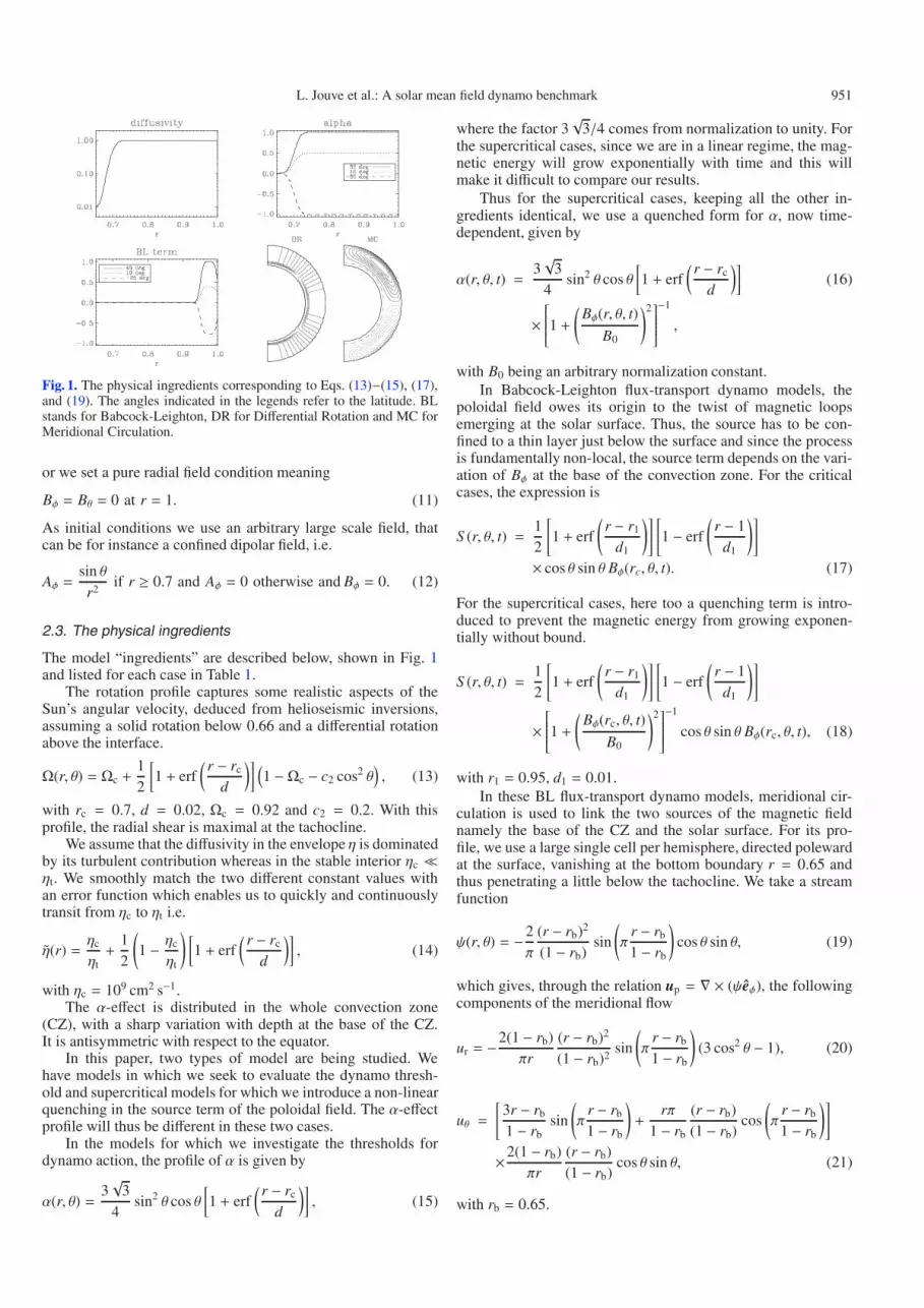
Fig. 1. The physical ingredients corresponding to Eqs. (13)−(15), (17),and (19). The angles indicated in the legends refer to the latitude. BLstands for Babcock-Leighton, DR for Differential Rotation and MC forMeridional Circulation.

or we set a pure radial field condition meaning

Bφ = Bθ = 0 at r = 1. (11)

As initial conditions we use an arbitrary large scale field, thatcan be for instance a confined dipolar field, i.e.

Aφ =sin θr2

if r ≥ 0.7 and Aφ = 0 otherwise and Bφ = 0. (12)

2.3. The physical ingredients

The model “ingredients” are described below, shown in Fig. 1and listed for each case in Table 1.

The rotation profile captures some realistic aspects of theSun’s angular velocity, deduced from helioseismic inversions,assuming a solid rotation below 0.66 and a differential rotationabove the interface.

Ω(r, θ) = Ωc +12

[1 + erf

( r − rc

d

)] (1 − Ωc − c2 cos2 θ

), (13)

with rc = 0.7, d = 0.02, Ωc = 0.92 and c2 = 0.2. With thisprofile, the radial shear is maximal at the tachocline.

We assume that the diffusivity in the envelope η is dominatedby its turbulent contribution whereas in the stable interior ηc ηt. We smoothly match the two different constant values withan error function which enables us to quickly and continuouslytransit from ηc to ηt i.e.

η(r) =ηc

ηt+

12

(1 − ηc

ηt

) [1 + erf

( r − rc

d

)], (14)

with ηc = 109 cm2 s−1.The α-effect is distributed in the whole convection zone

(CZ), with a sharp variation with depth at the base of the CZ.It is antisymmetric with respect to the equator.

In this paper, two types of model are being studied. Wehave models in which we seek to evaluate the dynamo thresh-old and supercritical models for which we introduce a non-linearquenching in the source term of the poloidal field. The α-effectprofile will thus be different in these two cases.

In the models for which we investigate the thresholds fordynamo action, the profile of α is given by

α(r, θ) =3√

34

sin2 θ cos θ[1 + erf

(r − rc

d

)], (15)

where the factor 3√

3/4 comes from normalization to unity. Forthe supercritical cases, since we are in a linear regime, the mag-netic energy will grow exponentially with time and this willmake it difficult to compare our results.

Thus for the supercritical cases, keeping all the other in-gredients identical, we use a quenched form for α, now time-dependent, given by

α(r, θ, t) =3√

34

sin2 θ cos θ[1 + erf

(r − rc

d

)](16)

×⎡⎢⎢⎢⎢⎢⎣1 +

(Bφ(r, θ, t)

B0

)2⎤⎥⎥⎥⎥⎥⎦−1

,

with B0 being an arbitrary normalization constant.In Babcock-Leighton flux-transport dynamo models, the

poloidal field owes its origin to the twist of magnetic loopsemerging at the solar surface. Thus, the source has to be con-fined to a thin layer just below the surface and since the processis fundamentally non-local, the source term depends on the vari-ation of Bφ at the base of the convection zone. For the criticalcases, the expression is

S (r, θ, t) =12

[1 + erf

(r − r1

d1

)] [1 − erf

(r − 1

d1

)]

× cos θ sin θ Bφ(rc, θ, t). (17)

For the supercritical cases, here too a quenching term is intro-duced to prevent the magnetic energy from growing exponen-tially without bound.

S (r, θ, t) =12

[1 + erf

(r − r1

d1

)] [1 − erf

(r − 1

d1

)]

×⎡⎢⎢⎢⎢⎢⎣1 +

(Bφ(rc, θ, t)

B0

)2⎤⎥⎥⎥⎥⎥⎦−1

cos θ sin θ Bφ(rc, θ, t), (18)

with r1 = 0.95, d1 = 0.01.In these BL flux-transport dynamo models, meridional cir-

culation is used to link the two sources of the magnetic fieldnamely the base of the CZ and the solar surface. For its pro-file, we use a large single cell per hemisphere, directed polewardat the surface, vanishing at the bottom boundary r = 0.65 andthus penetrating a little below the tachocline. We take a streamfunction

ψ(r, θ) = −2π

(r − rb)2

(1 − rb)sin

(π

r − rb

1 − rb

)cos θ sin θ, (19)

which gives, through the relation up = ∇ × (ψeφ), the followingcomponents of the meridional flow

ur = −2(1 − rb)πr

(r − rb)2

(1 − rb)2sin

(π

r − rb

1 − rb

)(3 cos2 θ − 1), (20)

uθ =

[3r − rb

1 − rbsin

(π

r − rb

1 − rb

)+

rπ1 − rb

(r − rb)(1 − rb)

cos

(π

r − rb

1 − rb

)]

×2(1 − rb)πr

(r − rb)(1 − rb)

cos θ sin θ, (21)

with rb = 0.65.

http://dexter.edpsciences.org/applet.php?DOI=10.1051/0004-6361:20078351&pdf_id=1


Table 1. Summary of the test cases, the cases followed by a prime have radial field boundary conditions (BC) at the top and the cases precededby S are supercritical (computed with a value of Cα or Cs well above the dynamo threshold).

Case Ω-effect Poloidal source term Diffusivity Meridional flow CΩ Cα Cs Re Top BC

A Eq. (13) α: Eq. (15) η = 1 (ηc = ηt in Eq. (14)) NO 1.40 × 105 Ccritα (A) 0 0 Potential

A′ Eq. (13) α: Eq. (15) η = 1 (ηc = ηt in Eq. (14)) NO 1.40 × 105 Ccritα (A′) 0 0 Radial

SA′ Eq. (13) α: Eq. (16) η = 1 (ηc = ηt in Eq. (14)) NO 1.40 × 105 3.5 0 0 RadialB Eq. (13) α: Eq. (15) Eq. (14) NO 1.40 × 105 Ccrit

α (B) 0 0 PotentialB′ Eq. (13) α: Eq. (15) Eq. (14) NO 1.40 × 105 Ccrit

α (B′) 0 0 RadialSB′ Eq. (13) α: Eq. (16) Eq. (14) NO 1.40 × 105 3.5 0 0 RadialC Eq. (13) BL: Eq. (17) Eq. (14) Eq. (19) 1.40 × 105 0 Ccrit

s (C) 700 PotentialC′ Eq. (13) BL: Eq. (17) Eq. (14) Eq. (19) 1.40 × 105 0 Ccrit

s (C′) 700 RadialSC′ Eq. (13) BL: Eq. (18) Eq. (14) Eq. (19) 1.40 × 105 0 35 700 Radial

2.4. Description of the test cases

Cases A and B are 2 different cases of pure αΩ dynamos, allusing the conical differential rotation profile (13) with a sharptachocline and an α-effect distributed in the whole convectionzone. Case A involves a constant diffusivity whereas in cases Band C, we introduce a diffusivity gradient between the core andthe envelope.

Case C is a Babcock-Leighton flux-transport dynamo, inwhich the source term for the poloidal field is due to the twistednature of active regions observed at the solar surface. The merid-ional circulation (MC) is introduced as one large single cell di-rected poleward at the surface, in accordance with solar obser-vations. In this model, we keep the magnetic diffusivity gradientand a solar-like differential rotation.

Cases A, B, C (A′, B′, C′) are computed with potential (ver-tical) field boundary conditions at the surface. Introducing thesetwo types of boundary condition will enable researchers who arenew to the field to test their codes with BCs whose implementa-tion can demand careful work.

In addition to these cases seeking to assess the dynamothreshold, we perform a more detailed comparison of the mag-netic field behaviour when the dynamo number has a value wellabove the dynamo threshold. These computations are also per-formed with radial field boundary conditions at the surface andwith a fixed resolution of 101×101 grid points. Since these casesare the supercritical cases of A′, B′ and C′, they are denotedas SA′, SB′ and SC′.

3. The codes involved

Eight different codes based on various numerical techniques areused to solve the mean field induction equation presented in thepreceding section. The main methods are finite differences, finiteelements and spectral decomposition. This enables this bench-mark to compare very different techniques representative of whathas been done as of today in the community to solve Eqs. (7)and (8). The codes are described briefly in this section and de-tailed descriptions can be found in the references given.

3.1. STELEM code

The STELEM (STellar ELEMemts) code uses a finite elementmethod in space and a third order scheme in time (Burnett 1987;Jouve & Brun 2007). The code solves Eqs. (7) and (8) by seek-ing the approximate solutions Aφ and Bφ as linear combinationsof trial functions ζi(r, θ) (Lagrange interpolating polynomials ofdegree 1 associated with the grid points (linear functions) for

1st order interpolation). The coefficients of the two linear com-binations are dependent on time only.

The main steps of the method are the following:

– Our domain (defined by rb ≤ r ≤ 1, 0 ≤ θ ≤ π) is di-vided into smaller regions called elements. These elementsare quadrilaterals with a node at each corner when the trialfunctions are 1st order Lagrange polynomials.

– In each element, the PDEs are transformed into ordinary dif-ferential equations in time involving the coefficients of thelinear combinations.

– The terms in the element equations are numerically evalu-ated for each element in the mesh. The resulting numbersare assembled into a much larger set of equations called thesystem equations.

– The boundary conditions are taken into account. They areimplemented here as Dirichlet type conditions: the topboundary condition is a potential field or purely radial field.We assume a perfectly conducting bottom boundary.

The temporal scheme that we use is adapted from Spalart et al.(1991). The 3 steps of this explicit scheme enable us to get anerror as small as O(∆t3) (see Jouve & Brun 2007; Charbonneau2005).

3.2. NDYND code

NDYND is a nonlinear dynamo code with density evolu-tion (the density does not evolve in our present calculations)(Brandenburg et al. 1992). It is an explicit code that solves themean field dynamo equations on a uniform mesh in r and θto second order. Advection-type terms are solved to fourth or-der. For mesh points on the boundaries, one-sided second orderderivative formulae are used whilst on the axis appropriate sym-metry conditions are used. Following Proctor (1977), the equa-tions are stepped forward in time using a second order Dufort-Frankel scheme that treats the diffusion operator semi-implicitly.The potential field boundary condition is implemented by calcu-lating the value of Aφ on the boundary through matrix multi-plication in terms of the values of two mesh points inside thedomain (Jepps 1975). The matrices are calculated prior to thesimulation for a given mesh. For case C described below, thevalue of Bφ(r = 0.7) is obtained by linear interpolation betweentwo neighbouring mesh points.

3.3. MBRK (Moss Brooke Runge-Kutta) code

This code integrates the dynamo equations over rb ≤ r ≤ 1,0 ≤ θ ≤ π, on a uniform 2-D grid. Spatial derivatives are sec-ond order, and time-stepping is by a second order Runge-Kutta


method (in tests, a fourth order Runge-Kutta scheme gave in-distinguishable results). When vacuum boundary conditions areused at the outer boundary, r = 1, a non-local matrix multipli-cation method is used (as in NDYND above). On other bound-aries, when needed, derivatives on the boundaries are evaluatedby their one-sided second order representations. In case C, thecoefficient Bφ(rc, θ) occurring in the source term is obtained bylinear interpolation from the neighbouring values. The code isbasically that of Moss & Brooke (2000).

3.4. MEFISTO (MEan FIeld STellar simulatiOn) code

The MEFISTO code solves the induction equation in a sphericalshell from rb to 1 and 0 ≤ θ ≤ π in radius and latitude, respec-tively (Käpylä et al. 2006). The grid is uniformly spaced andspatial derivatives are computed using explicit second order ac-curate finite differences. As time-stepping methods, either first-order Euler, or second order Adams–Bashforth schemes can beused. The boundary conditions are implemented using one-sidedexpressions of the first derivatives to yield the boundary value.For case C described above, the value of Bφ(rc, θ) is obtainedfrom linear interpolation between the adjacent grid points.

3.5. HAO Dynamo code1

The dynamo code of M. Rempel uses a fully explicit finite dif-ference scheme, which is second order in time and space (the ad-vection terms are discretized using a MacCormack scheme). Inits current version the code only supports a vertical field bound-ary condition at the surface. The code has been used recently byRempel (2006) to study non-linear Lorentz-force feedback ondifferential rotation and meridional flow. For the purpose of thisbenchmark study, the non-linear terms were switched off and thecode was used in a purely kinematic way. The results presentedin this paper were computed in only one hemisphere with sym-metry imposed through the equatorial boundary condition.

3.6. HAO Dynamo code2

The dynamo code of M. Dikpati numerically solves the two cou-pled partial differential equations of advection-diffusion type byusing a semi-implicit scheme, namely the Peaceman-Rachford-Alternating-Direction-Implicit scheme (Ames 1992; Press et al.1992). Writing the equations in operator notation as

∂Bφ

∂t= [Lr + Lθ] Bφ + S 1, (22)

∂A∂t= [Lr + Lθ] A + S 2, (23)

in which Lr contains all the operators in r and Lθ in θ and S 1and S 2 denote the cross-terms, the first half of the time-step isadvanced by treating the r-direction explicitly and θ-directionimplicitly, the next half time-step in the reverse manner. Thetime-step is determined by satisfying the CFL condition. Sincethe diffusive terms are parabolic, whereas the advective termsare hyperbolic, a space-centered finite differencing scheme forthe diffusive terms and a Lax-Wendroff scheme for the advectiveterms have been applied in order to maintain the second order ac-curacy in these mixed systems (see Dikpati 1996; and Dikpati &Charbonneau 1999 for more details regarding the calculations ofthe tridiagonal elements, initialization and boundary conditions).

3.7. CTDYN (Catania Dynamo) code

The dynamo code used for the benchmark is a pseudospectraleigenvalue code.

The induction equation is solved with a finite-differencescheme for the radial dependence and a Legendre polynomialexpansion for the angular dependence. In particular, the follow-ing expansions for the field is used

A(x, θ) = eλt∑

n

an(x) P(1)n (cos θ), (24)

B(x, θ) = eλt∑

m

bm(x) P(1)m (cos θ), (25)

where λ is the (complex) eigenvalue, n = 1, 3, 5, . . . and m =2, 4, 6, . . . for antisymmetric modes, and n ↔ m for symmet-ric modes. Vacuum boundary conditions at the surface and per-fectly conducting conditions at x = xi = 0.65 are then translatedinto simple ordinary differential equations involving the coeffi-cients an and bm.

By substituting (24) and (25) in the induction equation, aninfinite set of ODEs is obtained, that can be conveniently trun-cated in n when the desired accuracy is achieved. The systemis in fact solved by means of a second order accurate finite dif-ference scheme and the basic computational task is thus to nu-merically compute eigenvalues and eigenvectors of a block-banddiagonal real matrix of dimension M×n, M being the number ofmesh points and n the number of harmonics, M(α)v = λv and vis in general a complex eigenvector.

This basic algorithm is embedded in a bisection procedurein order to determine the critical dynamo number needed to finda purely oscillatory solution, for which e(λ) = 0 Numericallya zero is accepted when the dimensionless quantity e(λ)R2/ηt

is no greater than 10−3 in the following calculations. Greater ac-curacy usually requires a more refined spatial grid; see Bonanno(2004) for further details about the code.

3.8. HOLLERBACH code

The MHD code developed by Hollerbach (2000) is an incom-pressible, spherical, spectral scheme which solves the momen-tum equation, the induction equation, and the temperature equa-tion in the Boussinesq approximation. The dynamo benchmarkperformed by R. Arlt employs only the induction equation. FullMHD computations of the magnetorotational instability withthis code are given in Arlt et al. (2003).

The magnetic field is decomposed into two scalar potentials,g and h, defined by

B = ∇ × (ger) + ∇ × ∇ × (her), (26)

where er is the radial unit vector. The potentials depend on r,θ, and φ. The actual equations being solved are the radial com-ponent of the induction equation and the radial component ofthe curled induction equation. The potentials g and h are usedin their spectral representation with spherical harmonics for theazimuthal and latitudinal structure, such that

g(r, θ, φ) =±M∑m=0

L∑l=m′

glm(r, t)P|m|l (cos θ)eimφ, (27)

where m′ = max(m, 1) and L and M are the truncations of thespectral expansion. In this paper, we set M = 0 for all com-putations because of axisymmetry. Finally, these expressions


are reintroduced in the induction equation which is integratednumerically.

The radial dependence of g and h is further expanded inChebyshev polynomials which have a high density of zeros nearthe radial boundaries, hence providing very good resolution inthe boundary layers. Two additional modes are used to imple-ment the radial boundary conditions for the magnetic field. Thephysical condition for a boundary with vacuum is ∇ × B = 0for the exterior and leads to particular conditions for g and h andlikewise for the conditions for perfectly conducting boundaries.

The diffusive part of the system is solved implicitly. Thetime-stepping is a Runge-Kutta integration with a second orderpredictor and corrector steps. While the determination of criti-cal dynamo numbers of α-type dynamos is a linear problem, wehave kept the scheme in order to be able to add nonlinearitiessuch as quenching functions or nonlocality to the source term S .

The non-linear routine consists of a transformation of thespectral potentials into a real-space B, the computation of U×B+S , and the curling and back-transformation into spectral space.The velocity field U and the source term S are only defined inreal space.

4. Results

The goal of this benchmark is to publish a detailed analysis ofthe results obtained by 8 different codes running on well-definedtest cases and to quantitatively assess the agreement between thecodes. It aims at providing the community with precise standardsolar dynamo cases to which to refer. In order to compare ourresults both qualitatively and quantitatively, we indicate in ta-bles for each case the critical dynamo number Ccrit

α above whichthe solution is growing exponentially, and the corresponding fre-quency ω, defined by ω = 2π/T with the magnetic cycle pe-riod T (i.e. twice the period of the sunspot cycle) in terms ofthe diffusive time R2/ηt. In addition to these quantitative results,we provide the butterfly diagrams and the evolution of the fieldlines in a meridional plane for each case, in order to follow thebehaviour of the magnetic field configuration over time. For thesupercritical cases, since the intensity of the magnetic field issaturated through the quenching term, we can perform a detailedcomparison of the field intensity at selected points in the compu-tational domain during a part of the cycle. We can then see thedeviation of each curve obtained by the different codes from themean curve, which will be considered to be the “optimal solu-tion”. Finally, to confirm that all codes converge to the same so-lution, we run convergence tests for 2 particular cases (B and C′),which allow us to follow the evolution of the values of Cα or Csand ω as the spatial resolution is increased.

4.1. Case A

4.1.1. Critical cases

Table 2 shows the results for the critical dynamo numbers andperiods for cases A and A′. The results are in good agreementwith each other, the relative standard deviation reaching only thevalue of 0.006 for Cα in both cases, meaning that the values areall gathering close to the mean. The agreement on the period isalso quite satisfactory, the relative standard deviation being againof the order of a few parts in a thousand.

In these cases, we find that only relatively low spatial res-olution is needed for convergence and close agreement. Eventhough the error function representations of α and Ω imply rel-atively rapid changes in these functions, they are smooth and

Table 2. Critical values of dynamo numbers and frequencies for caseA (with potential boundary conditions) and case A′ (with radial fieldconditions) with the spatial and temporal resolution for each code. Weindicate the mean value, the standard deviation and the relative standarddeviation (R.S.D) (standard deviation divided by the mean value) foreach case. Asterisks indicate particular cases: for HOLLERBACH, theresolution is given in terms of the number of spectral modes and forCTDYN in terms of grid points in r and spectral modes in θ. CTDYNdoes not evolve the system in time, which is why we do not indicate anytime-step for this code.

Case Code Resolution ∆t Ccritα ω

A STELEM 65 × 65 10−5 0.385 157A NDYND 81 × 81 5 × 10−6 0.385 158A MBRK 81 × 81 5 × 10−6 0.390 159A CTDYN 70 × 70 * – 0.388 160A HAO2 101 × 101 10−5 0.388 156A HOLLER 60 × 60 * 5 × 10−5 0.385 159

Mean val 0.387 158.1Std Dev. 0.002 1.472R. S. D. 0.006 0.009

A′ STELEM 65 × 65 10−5 0.366 158A′ NDYND 81 × 81 5 × 10−6 0.369 156A′ MBRK 81 × 81 5 × 10−6 0.372 158A′ MEFISTO 121 × 121 10−6 0.368 158A′ HAO1 128 × 128 3 × 10−6 0.368 157


t=0.115 t=0.118 t=0.122

t=0.125 t=0.130 t=0.135

CASE A

Fig. 2. Results for case A: pure αΩ dynamo with constant magneticdiffusivity. The results are shown for Cα = Ccrit

α . The figure shows theevolution of the contours of the poloidal potential (left panel) and ofthe toroidal field (right panel) during half a magnetic cycle. Red (blue)colours indicate positive (negative) toroidal field and plain (dotted) linesindicate clockwise (anticlockwise) poloidal field lines.

the models do not produce strong radial or latitudinal gradi-ents in the induced toroidal or poloidal fields. Instead, the mag-netic fields are organized in very large structures that smoothlymatch the boundary conditions. Since these solutions occur fordynamo numbers only slightly above critical, no strong gradientsin toroidal or poloidal fields should arise at later times either. Wesee that the solutions satisfying radial field boundary conditionsat r = 1 are excited at lower dynamo numbers than for the po-tential field boundary conditions. But the dynamo frequency isnearly the same for both boundary conditions, about 158 (cor-responding to a period of 30.9 years in dimensional units, com-pared to 11 years for the solar cycle). Figures 2 and 3 show the



Fig. 3. Case A: butterfly diagram i.e. time-latitude cut of the toroidalfield at 0.7 R (upper panel) and of the radial field at the surface (lowerpanel). Red (blue) colours indicate positive (negative) values of thefield.

Fig. 4. Same as case A but for case SA′.

behaviour of the solution over time. Figure 2 shows the evolutionof the field lines in the meridional plane in the northern hemi-sphere during half a magnetic cycle and Fig. 3 shows a time-latitude cut of the toroidal field at the base of the convectionzone (r = 0.7) and of the radial field at the surface in both hemi-spheres. In this case the solution produces a butterfly diagramwhose “wings” for the toroidal field slope toward the poles withincreasing time, opposite to the solar case.

4.1.2. Supercritical case

We have previously discussed models A and A′ in the case whereCα was at its critical value, i.e. in the case of a quasi-stationarymagnetic energy. We now compare the various codes for a su-percritical case of model A′ (with vertical field conditions at thesurface). We thus choose for this case a value of Cα of 3.5, al-most 10 times the critical value of Cα in this case.

Figure 4 represents the butterfly diagram obtained in caseSA′. The evolution of the magnetic field is close to what wefound for the critical case. We can nevertheless notice that thehigh latitude polar branch is reduced in this case compared tocase A but, in the latitudinal band where the sunspots appear, weagain see that the toroidal field is moving poleward, contrary towhat is observed in the Sun. We also see that increasing the Cα

decreases the cycle period in this case.Figure 5 shows the deviation from the mean value of cuts

at various radii and latitudes of the toroidal and radial fields inthe magnetic energy-saturated regime for the different codes. Allcurves were adjusted so that Bφ at the base of the convection

Fig. 5. Case SA′: comparison between the values of Bφ(r =0.7, latitude = 60) and Br(r = 1, latitude = 30) normalized by B0

obtained by the different codes during a cycle. The right panels show azoom on the first maximum of the field and on the first time the field re-turns to zero after one cycle period. The thick line represents the meanvalue of the field and the coloured lines represent the curves obtained bythe different codes. The colour coding is the following: HAO1 in blue,MBRK in red, STELEM in green, NDYND in black dashed, HAO2 inblack and MEFISTO in black dotted.

zone is exactly 0 at t = 0. We show for each curve a zoom on thefirst maximum of Bφ at the base of the convection zone and of Brat the solar surface and on the crossing of zero after one cycleperiod. This procedure enables us to compare both the amplitudeshift and the phase shift caused by the various codes.

We first see that the deviations between the codes are moresignificant for Br at the surface. This could be due to various ef-fects such as the imposition of the boundary conditions or thesharper profile of Br close to its maximum compared to Bφ.Nevertheless, the deviation from the mean curve stays under 7%of the maximum value of the field and this deviation drops toabout 1.2% for Bφ. The agreement on the field maxima is thusvery satisfactory.

Looking at the instant where Bφ and Br return to zero afterone period enables us to see the significance of the phase shiftbetween the various solutions. Again the differences are morepronounced for the curves for the radial field. The curves allcross zero in the very small time interval [0.0444, 0.0450] whichis about 1.6% of the cycle period. The length of this time intervalis the same for the curves for the toroidal field.

This pure αΩ dynamo model includes a constant magneticdiffusivity. This ingredient of the model is one of the most poorlyknown but we can reasonably assume that the net diffusivityshould be much lower in the convection-free radiative core thanin the turbulent envelope and thus that the diffusivity should varywith depth in our computational domain. In the following case,we refine our model to test the influence of applying a gradientof magnetic diffusivity in a pure αΩ model and how the variouscodes cope with this more challenging computation.




Table 3. Same as for Table 2, for cases B and B′.


B STELEM 129 × 129 10−6 0.410 172B NDYND 81 × 81 10−5 0.405 172B MBRK 128 × 128 10−6 0.411 172B CTDYN 70 × 70 * – 0.411 172B HAO2 101 × 101 10−5 0.403 171B HOLLER 60 × 60 * 5 × 10−5 0.408 173

Mean val 0.408 172Std Dev. 0.003 0.632R. S. D. 0.008 0.004

B′ STELEM 65 × 65 10−5 0.387 169B′ NDYND 81 × 81 10−5 0.385 168B′ MBRK 128 × 128 10−6 0.391 169B′ MEFISTO 121 × 121 10−6 0.387 169B′ HAO1 128 × 128 3 × 10−6 0.387 169


4.2. Case B

In this case, the magnetic diffusivity is no longer constant, as in-dicated by Eq. (14). This refinement enables us to test how thevarious codes cope with a non constant diffusivity profile inthe model. Here again, the comparison is made by looking atthe critical Cα, at the periods, and at the strength of the magneticfield during one cycle.


As Table 3 shows, the agreement of all codes on the critical val-ues of Cα is quite good, even at low resolution. We note that thediffusivity gradient makes it more difficult for the dynamo to beexcited and produces shorter cycles (see Table 2 for a close com-parison with case A), indeed the frequency is now close to 170,which corresponds to a sunspot period of 28.7 years, given ourchoice of ηt.

We note again that in this case the dynamo is more easilyexcited when radial BCs are imposed, and that the period of thedynamo waves is slightly increased in case B′. Moreover, theagreement on the value of the critical dynamo number is betterin case B′, showing that the imposition of potential boundaryconditions can induce some divergence between codes. We thenconclude that, even in this simple αΩ model the choice and im-plementation of boundary conditions can already be a delicateissue.

Figure 6 indicates the convergence behaviour of each codetoward the values quoted in Table 3 for case B with potentialBCs. Note that for each quantity (Ccrit

α and ω), the spread of thevalues in the converged part of the diagram is less than 1% ofthe absolute value. That is, all results that fall in the diagramagree within better than 1%, as we can already see in Table 3.All results seem to converge approximately towards the samepoint, especially for the frequency, where the agreement is ex-tremely good. We note that in this case, most codes have alreadyconverged with a resolution of 80 × 80, confirming that this cal-culation does not require a very high resolution in spite of thesharp diffusivity profile and the imposition of potential bound-ary conditions. We note that the convergence is very fast for thepseudospectral code CTDYN, since the values at a resolution of40 × 40 are already close to the converged value.

Fig. 6. Convergence test for case B: evolution of the values of Ccritα andω

as functions of the spatial resolution. The colour coding is the follow-ing: HAO2 in black, CTDYN in blue, STELEM in green, MBRK inred, HOLLER in light green for which the resolution is the number ofcollocation points, twice the number of Chebyshev polynomials.

CASE B

t=0.115 t=0.118 t=0.122

t=0.125 t=0.130 t=0.133

Fig. 7. Same as Fig. 2 but for case B: pure αΩ dynamo with a jumpof magnetic diffusivity from 0.01ηt below the tachocline to ηt in theconvection zone. The results are shown for Cα = Ccrit

α .

As we can see in Figs. 7 and 8, the magnetic field be-haviour is close to what was found in the constant diffusivitycase (case A) except that the poloidal field lines seem to be lessdiffuse in the tachocline due to the presence of the sharp diffu-sivity gradient in this zone. In the meridional plane, the regionsof generation and destruction of the magnetic structures are thesame and the directions of rise and migration of the field areidentical to case A. However, we notice in the butterfly diagramthat the regions of strongest magnetic intensity are confined ina much smaller region around 30 latitude approximately in theregion of strongest α-effect. The polar branch at high latitudes(above 60) of the toroidal field is more stretched in time andless intense compared to the regions of strongest intensity thanin case A. The addition of variable diffusivity and thus of diffu-sivity gradients have some impact on the field location and itsorganization in finer structures.




Fig. 8. Same as Fig. 3 but for case B.

Fig. 9. Same as Fig. 4 but for case SB′: supercritical case of pure αΩdynamo with variable diffusivity: butterfly diagram i.e. time-latitude cutof the toroidal field at 0.7 (upper panel) and of the radial field at thesurface (lower panel).


Figure 9 shows the butterfly diagram obtained in case SB′. Itis again very similar to case SA′ shown in Fig. 4; we indeedrecover the poleward migration of the toroidal field, with a pole-ward branch at high latitudes being a little more pronounced thanin case SA′. This was also one of the main differences betweencase A and case B.

Figure 10 shows the comparison between the values of thetoroidal and radial fields at a specific latitude and radius. Theagreement is again very reasonable between all codes. Indeed,the difference between the various curves is hardly distinguish-able if we do not zoom in on particular areas of the graphs.Zooming on the maximum of Bφ indicates that the deviationsfrom the mean curve do not exceed 1.5% of the maximum valueof the field. The phase shift is also very small, all curves recoverthe instant of zero-crossing quite well. If we do not take into ac-count the extreme curve, which is a little further from the meancurve, we find the deviation does not exceed 0.6% of the meanvalue. This extremely small value indicates that the codes canreproduce very precisely the cycle period.

The agreement between all codes for the radial field at lati-tude= 30 at the surface is reduced compared to the toroidal fieldat latitude= 60 at the base of the convection zone. Nevertheless,the deviation from the mean curve stays under 3%, despite thevery sharp profile of Br when it reaches its maximum. The de-viations at the instant where Br vanishes after one cycle do notexceed 3.5% of the cycle period. Most of the curves are locatedso close to each other that it is difficult to distinguish them even

Fig. 10. Same as Fig. 5 but for case SB′.

on the zoomed frame, where the range represents only about 9%of the cycle period.

The agreement in cases A and B of αΩ dynamos are thusvery satisfactory, despite the strong gradients of α, Ω and ofmagnetic diffusivity in case B. We now compare a completelydifferent solar dynamo model which includes the meridional cir-culation, the large scale flow which is observed in the Sun andwhich may play a role in the dynamo loop.

4.3. Case C

Case C is a Babcock-Leighton flux-transport dynamo which in-corporates a solar-like differential rotation, magnetic diffusivitysharply varying with depth, meridional circulation and a non-local Babcock-Leighton source term for the poloidal field. Thismodel thus takes into account two observed solar features whichmay play a role in dynamo action: meridional flow and thetwist of active regions at the surface. As we wish to be in theadvection-dominated regime, we want an efficient connectionbetween the magnetic field source regions (the base of the CZand the surface) by means other than magnetic diffusion, i.e. themeridional circulation (see Eq. (19)). Moreover, in this model,the poloidal field owes its origin to the twisted nature of activeregions at the solar surface due to the Coriolis force, which isagain an observed feature of the solar magnetic activity. Thismechanism is modeled by the non-local surface source term S ofEq. (17) which appears in the equation for the evolution of Aφ.


Looking at Table 4, we notice that cases C and C′ require morespatial and temporal resolution for convergence than the αΩcases. A high resolution is needed to obtain a reasonably goodagreement between all codes.

The imposition of radial field boundary conditions in caseC′ can partly explain the high resolution needed. At the surface,the poloidal field and consequently Bθ is created and the outerboundary conditions force the component Bθ to be zero. Thelatitudinal component of B thus has to move smoothly from anon-zero value in a thin layer below the surface to zero at the



Table 4. Same as for Table 2, for cases C and C′.


C STELEM 129 × 129 10−6 2.520 542C NDYND 81 × 81 10−6 2.513 525C HAO2 101 × 101 10−5 2.515 546C MBRK 151 × 151 10−6 2.540 532C HOLLER 100 × 100 * 5 × 10−8 2.355 538


C′ STELEM 129 × 129 10−6 2.460 544C′ NDYND 321 × 321 5 × 10−7 2.469 534C′ MBRK 256 × 256 5 × 10−7 2.473 537C′ MEFISTO 201 × 201 10−6 2.463 539C′ HAO1 128 × 128 3 × 10−6 2.450 537


Fig. 11. Same as Fig. 6 but for case C′. The colour coding is now thefollowing: STELEM in green, NDYND in black dashed, MBRK in red,HAO1 in blue and MEFISTO in black dotted.

surface, which requires the resolution to be sufficient to handlethis strong gradient.

The dispersion of the values for Ccrits in case C is higher than

in the previous cases but the relative standard deviation is de-creased from 3% to 0.5% if we remove the value of 2.355 of theHOLLERBACH code, which is quite far from the other results.The cycle frequency is also sensitive to the numerical methodused, although all codes agree to within less than 2%. We notethat the agreement is increased in case C′, when radial boundaryconditions are used.

This more sophisticated flux-transport model (in compari-son to the previous αΩ models) leads to a higher though stillreasonable dispersion of the values. This higher dispersion is tobe expected, since this case includes a meridional flow and anon-local source term for the poloidal field and is therefore nu-merically more challenging.

Figure 11 shows the convergence behaviour of each code to-ward the values quoted in Table 4 for case C′. Again, the agree-ment among the various codes is very satisfactory, the spread ofthe values in the converged part of the diagrams is less than 1%

CASE C

t=0.116 t=0.117 t=0.118

t=0.119 t=0.120 t=0.122

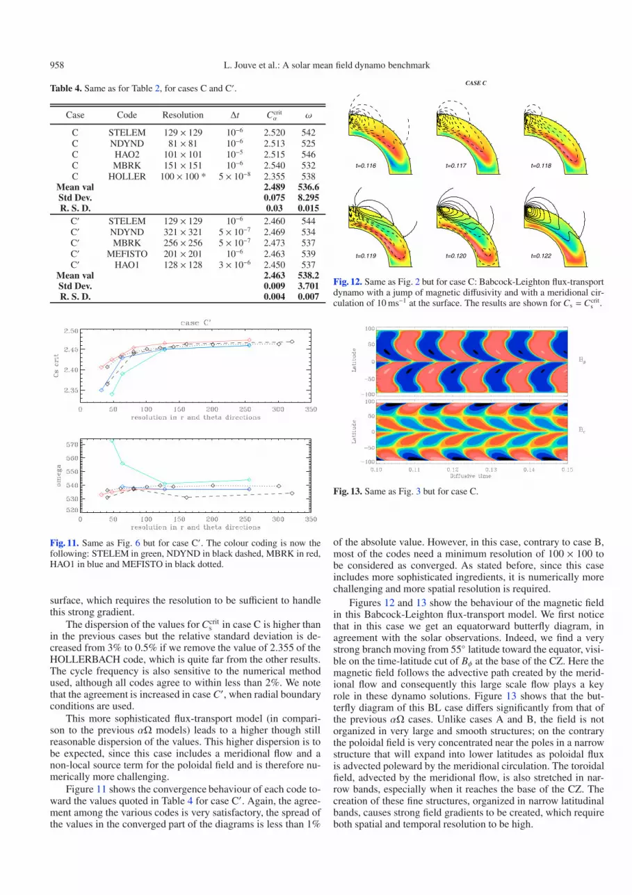
Fig. 12. Same as Fig. 2 but for case C: Babcock-Leighton flux-transportdynamo with a jump of magnetic diffusivity and with a meridional cir-culation of 10 ms−1 at the surface. The results are shown for Cs = Ccrit

s .

Fig. 13. Same as Fig. 3 but for case C.

of the absolute value. However, in this case, contrary to case B,most of the codes need a minimum resolution of 100 × 100 tobe considered as converged. As stated before, since this caseincludes more sophisticated ingredients, it is numerically morechallenging and more spatial resolution is required.

Figures 12 and 13 show the behaviour of the magnetic fieldin this Babcock-Leighton flux-transport model. We first noticethat in this case we get an equatorward butterfly diagram, inagreement with the solar observations. Indeed, we find a verystrong branch moving from 55 latitude toward the equator, visi-ble on the time-latitude cut of Bφ at the base of the CZ. Here themagnetic field follows the advective path created by the merid-ional flow and consequently this large scale flow plays a keyrole in these dynamo solutions. Figure 13 shows that the but-terfly diagram of this BL case differs significantly from that ofthe previous αΩ cases. Unlike cases A and B, the field is notorganized in very large and smooth structures; on the contrarythe poloidal field is very concentrated near the poles in a narrowstructure that will expand into lower latitudes as poloidal fluxis advected poleward by the meridional circulation. The toroidalfield, advected by the meridional flow, is also stretched in nar-row bands, especially when it reaches the base of the CZ. Thecreation of these fine structures, organized in narrow latitudinalbands, causes strong field gradients to be created, which requireboth spatial and temporal resolution to be high.




Fig. 14. Same as Fig. 4 but for case SC′.

Fig. 15. Same as Fig. 5 but for case SC′.


Increasing Cs to 35 (about 14 times supercritical for dynamoaction) enables us to see the fields in the regime of a well-established flux-transport dynamo.

Figure 14 shows that the associated butterfly diagram for thetoroidal field is similar to case C shown in Fig. 13. Some differ-ences are nevertheless visible in the evolution of the radial fieldat the surface, like the appearance of finer structures close to theequator.

In this flux-transport model, the physical ingredients aremore sophisticated and thus the uncertainty on the critical Cs andon the cycle period seems to be more significant. Nevertheless,as Fig. 15 shows, the agreement on the values of the toroidal andradial field at specific points is again very good. The deviationfrom the mean curve is of the order of 1% for both the maximain the toroidal fields and for the differences in phase.

This time, the agreement on the behaviour of the radial fieldin one cycle period is as good as the agreement in the toroidalfield. Both the maximum of the field and the instant where Brvanishes are very well reproduced and are very close to the mean“optimal” solution.

5. Conclusions

Understanding the activity and magnetic cycle of the Sun is cru-cial since its variability has a direct impact on our technologicalsociety by disturbing high frequency signals, impairing satellitesand damaging power grids. For decades the scientific communityhas developed observational, theoretical and numerical tools inorder to be able to understand the inner workings of the Sun,while at the same time aiming to be able to predict its activity.The current accepted scenario states that this surface magnetismis linked to an internal dynamo. Two dimensional mean field dy-namo models have proved to be very useful tools to test and val-idate ideas and distinguish among scenarios of the solar dynamosuch as αΩ, α2 or flux-transport and to progress in our effort tounderstand the Sun as a whole.

The inclusion of the meridional circulation in the dynamotheory of the solar cycle turns out to be essential in reproducingthe most important features of the 11-yr cycle. On the other handif the eddy diffusivity ηt is as low as 1011 cm2 s−1, the magneticReynolds number Re = u0R/ηt reaches values of the order of103 for a flow of about 10 ms−1.

How robust then are the predictions of dynamo codes forpurely kinematic models? In this paper eight different codes,based on finite differences, finite elements and spectral decom-position, have been considered in order to solve the 2D inductionequation in spherical geometry in the presence of strong gradi-ents of the turbulent diffusivity, a realistic differential rotationprofile and high magnetic Reynolds numbers. Again, the casesdiscussed in this paper are not intended to exhaustively coverall the solar dynamo models that have been published in the lit-erature so far, such as non-linear Malkus-Proctor models (seee.g. Brandenburg et al. 1991; Moss & Brooke 2000; or Bushby2006). However, we believe that the cases chosen are represen-tative of typical mean field kinematic dynamo models.

By defining three standard solar dynamo cases, namelycases A, B and C that are made increasingly more sophisticatedby introducing well defined physical ingredients, we hope tohave been able to provide useful test models easily reproducibleby anyone seeking to validate their code. Cases A, B and Chave potential boundary conditions on top of the domain. Similarcases are computed using radial field boundary conditions (casesA′, B′ and C′) since the imposition of BCs are known to bea delicate issue and is consequently a phase of code develop-ment that also needs to be carefully validated. For each case welist in summary tables the ingredients used, the critical dynamonumber for the onset of dynamo action, and the resulting cycleperiod for each code. Moreover, we display typical realizationsof the poloidal and toroidal fields in the meridional plane overhalf a cycle and butterfly diagrams of the toroidal field at thebase of the convection zone as well as the radial field at thesurface. In order to show that the solutions of these test casesare confirmed by several independent codes and are convergedto high accuracy, we show convergence plots for two particularcases B and C′. Further, for each set of parameters chosen, wecompute supercritical cases (SA′, SB′ and SC′) including non-linear quenching of the poloidal source term (the α effect forcases A and B and the Babcock-Leighton term for case C) at afixed resolution of 101 × 101 and display the butterfly diagramobtained in that high dynamo number regime. In order to facil-itate a more quantitative analysis of the results of the variouscodes, we plot for six of the eight codes used in this study spe-cific cuts of the toroidal and radial fields at fixed latitude andradius. Given the quite good agreement between the differentsolutions obtained with the various numerical codes, these later


figures serve two purposes: a) they help in determining the in-trinsic deviation among all codes and b) they allow a quantitativecomparison of the prediction made by the codes for the strengthof the radial and toroidal fields in the numerical domain.

The key point to be extracted from our analysis is that theagreement between the different codes used in this benchmarkstudy is indeed quite good, being of the order of (or even lessthan) 1% for the reference αΩ dynamo cases A and B, in spiteof the non-trivial pattern of differential rotation and for case Bthe presence of a strong gradient of the turbulent diffusivity. Itis also important to note that in the search for critical values ofthe dynamo numbers, the eigenvalue code and the time-evolvingcodes agree rather well.

When the meridional flow is present as in case C, the agree-ment is still reasonably good but with a dispersion of the or-der of a few percent in the values of the critical dynamo num-ber and in the periods. This case includes meridional flow, asolar-like differential rotation, a sharp tachocline, a gradient ofmagnetic diffusivity and a non-local source term for the poloidalfield. It is thus numerically more challenging and requires moreresolution to converge, whatever the numerical technique used.Nevertheless the values of the toroidal field at the base of theconvection zone and the butterfly diagrams are very well repro-duced by all the codes for all the cases considered.

We anticipate that the well-documented benchmark casespresented here will be a useful tool for any researcher who in-tends to develop/validate his/her code, since they provide stan-dard cases to which to refer and detailed tables and figures for aquantitative comparison.

Acknowledgements. We wish to thank the International Space Science Institute(ISSI) for supporting our international team with the program: observations andmodels of the solar cycle. M.D. acknowledges financial support from NASAgrant NNH05AB521 and the NCAR Director’s opportunity fund.

References

Ames, W. F. 1992, Numerical Methods for Partial Differential Equations,3rd edn. (San Diego: Academic), Chap. 3

Arlt, R., Hollerbach, R., & Rüdiger, G. 2003, A&A, 401, 1087

Babcock, H. W. 1961, ApJ, 133, 572Bonanno, A. 2004, Mem. Soc. Astron. It., 4, 17Bonanno, A., Elstner, D., Rüdiger, G., & Belvedere, G. 2002, A&A, 390,

673Brandenburg, A., Moss, D., Rüdiger, G., & Tuominen, I. 1991, Geophys.

Astrophys. Fluid Dyn., 61, 179Brandenburg, A., Moss, D., & Tuominen, I. 1992, A&A, 265, 328Browning, M. K., Miesch, M. S., Brun, A. S., & Toomre, J. 2006, ApJ, 648,

L157Brun, A. S., Miesch, M. S., & Toomre, J. 2004, ApJ, 614, 1073Burnett, D. S., 1987, Finite Element Analysis (Addison-Wesley)Bushby, P. J. 2006, MNRAS, 371, 772Cattaneo, F. 1999, ApJ, 515, L39Charbonneau, P. 2005, Liv. Rev. Sol. Phys., 2, 2Choudhuri, A. R., Schüssler, M., & Dikpati, M. 1995, A&A, 303, L29Dikpati, M. 1996, Ph.D. Thesis, Indian Ins. Sci., BangaloreDikpati, M., & Charbonneau, P. 1999, ApJ, 518, 508Dikpati, M., & Gilman, P. A. 2006, ApJ, 649, 498Dikpati, M., de Toma, G., Gilman, P. A., Arge, C. N., & White, O. R. 2004, ApJ,

601, 1136Durney, B. R. 1995, Sol. Phys., 160, 213Gilman, P. A. 1983, ApJS, 53, 243Glatzmaier, G. A. 1987, The Internal Solar Angular Velocity, ed. B. R. Durney,

& S. Sofia (Dordrecht: D. Reidel), 263Hollerbach, R. 2000, Int. J. Numer. Meth. Fluids, 32, 773Jepps, S. A. 1975, J. Fluid Mech., 67, 625Jouve, L., & Brun, A. S. 2007, A&A, 474, 239Käpylä, P. J., Korpi, M. J., & Tuominen, I. 2006, AN, 327, 884Krause, F., & Rädler, K. H. 1980, Mean Field Magnetohydrodynamics and

Dynamo Theory (Oxford: Pergamon Press)Küker, M., Rüdiger, G., & Schultz, M. 2001, A&A, 374, 301Leighton, R. B. 1969, ApJ, 156, 1Moffatt, H. K. 1978, Magnetic field Generation in Electrically Conducting Fluids

(Cambridge University Press)Moss, D., & Brooke, J. 2000, MNRAS, 315, 521Press, W. H., Teukolsky, S. A., Vetterling, W. T., & Flannery, B. P. 1992,

Numerical Recipes, 2nd edn. (Cambridge: Cambridge Univ.)Proctor, M. R. E. 1977, J. Fluid Mech., 80, 769Rempel, M. 2006, ApJ, 647, 662Roberts, P. H. 1972, Phil. Trans. R. Soc. London, 272, 663Spalart, P. R., Moser, R. D., & Rogers, M. M. 1991, Comp. Phys., 96, 297Steenbeck, M., & Krause, F. 1969, AN, 291, 49Steenbeck, M., Krause, F., & Rädler, K. H. 1966, Z. Naturforsch. Teil A, 21,

369Stix, M. 1976, A&A, 47, 243Wang, Y.-M., Sheeley, N. R., Jr., & Nash, A. G. 1991, ApJ, 383, 431

A solar mean field dynamo benchmark

Documents

Transcript of A solar mean field dynamo benchmark