SPECTROSCOPIC MEASUREMENT OF THE MHD DYNAMO

IN THE MST REVERSED FIELD PINCH

by

James Tharp Chapman

A dissertation submitted in partial fulllment of the

requirements for the degree of

Doctor of Philosophy

(Physics)

at the

University of WisconsinMadison

1998

i

SPECTROSCOPIC MEASUREMENT OF THE MHD DYNAMO

IN THE MST REVERSED FIELD PINCH

James Tharp Chapman

Under the supervision of Professor Stewart C. Prager

At the University of WisconsinMadison

Abstract

We have directly observed the coupling of ion velocity uctuations and magnetic

eld uctuations to produce an MHD dynamo electric eld in the interior of the MST

reversed eld pinch. Chord averaged ion velocity uctuations were measured with a fast

spectroscopic diagnostic which collects line radiation from intrinsic carbon impurities

simultaneously along two lines of sight. The chords employed for our measurements re-

solved long wavelength velocity uctuations of several km/s at 820 kHz as tiny, fast

Doppler shifts in the emitted line prole. During discrete dynamo events the veloc-

ity uctuations, like the magnetic uctuations, increase dramatically. The toroidal and

poloidal chords with impact parameters of 0:3 a and 0:6 a respectively, resolved uctua-

tion wavenumbers with resonance surfaces near or along the lines of sight indicating a

radial velocity uctuation width for each mode which spans only a fraction of the plasma

radius. The phase between the measured toroidal velocity uctuations and the magnetic

uctuations matches the predictions of resistive MHD while the poloidal velocity uctua-

tions exhibit a phase consistent with the superposition of MHD eects and the advection

of a mean ow gradient past the poloidal line of sight. Radial velocity uctuations re-

ii

solved by a chord through the center of the plasma were small compared to the poloidal

and toroidal uctuations and exhibited low coherence with the magnetic uctuations.

The ensembled nonlinear product of the ion velocity uctuations and uctuations in the

magnetic eld indicates a substantial dynamo electric eld which peaks during the pe-

riods of spontaneous ux generation. During these periods our measurements indicate

poloidal dynamo eld of 147 Volts/m near the plasma core in the direction to generate

toroidal ux and a small toroidal dynamo eld in the edge region of 1.00:3 Volts/m in

the direction to drive parallel current. While the absolute magnitudes of the observed

dynamo elds are consistent with estimates from equilibrium modeling, discrepancies

which remain indicate the need for additional dynamo measurements to demonstrate the

numerical balance of parallel Ohm's law by a dynamo electric eld the the reversed eld

pinch.

iii

Acknowledgments

Through the course of my graduate studies I have been supported by the faculty,

sta and students of the MST group. I acknowledge below the contributions of those who

have enabled the work presented in this thesis and enriched the environment in which it

was produced.

Prof. Prager helped me extract interesting physics from the tangled web of diagnos-

tic, analysis, and computational issues and provided a careful reading and editing of this

thesis. Dan Den Hartog brought me into this group six years ago by requesting an Na-

tional Undergraduate Fellow and has since provided mentoring in the careful techniques

of experimental physics, willing consideration of research results and plans, opportunities

to present work in papers and talks, exibility in responding to personal requests, and a

remarkable diagnostic described in some detail in Chapter 2 of this thesis. The rest of

the MST faculty and scientic sta has never failed to open their doors to my questions

and ideas: John Sar helped iron out the technical minutiae of mode analysis and equi-

librium modeling; Abdul Almagri provided his magnetic probe, good humor, and skills

as a butcher; Gennady Fiksel oered creative experimental ideas many of which actually

worked; and Prof. Cary Forest provided a fresh critical perspective which induced some

reworking and some rethinking and ultimately contributed to a better piece of research.

The MST technical and engineering sta have been unselsh with their time and

expertise: Tom Lovell, Mark Thomas, and Steve Oliva gave assistance back when I

was building stu and/or putting stu on the machine; John Laufenberg answered the

phone on the weekends when we couldn't gure out what was wrong with the MST;

Bill Zimmerman, Tom Krajewski, Doug Drescher, and Mikhail Reyfman helped me nd

the little things I was always looking for; and Roch Kendrick proofread my drawings

so they would become neither a source of amusement nor a cause of annoyance in the

machine shop. The volume data analysis involved in my research occasionally taxed

the computational resources and possibly the patience of Larry Smith and Paul Wilhite

although both maintained their sense of humor and appeased me (nally!) with a really

iv

nice computer. Dale Schutte got the orders out on time when I purchased several times

my personal net worth in parts from Digi-Key and Newark. Kay Shatrawka graciously

helped me get through the details and postpone the days work a few minutes with

conversation over coee.

The MST graduate students and post-docs provided a fantastic work and social

environment. They include: Jay Anderson, who killed my Frankenstein and conquered

the world from Australia; Ted Biewer, my partner in crime through the S-scale run;

Brett Chapman, who withstood my repeated attempts to log into his VAX account;

(Lt.) Ching-Shih Chiang, the nicest guy to ever violate MST vacuum protocol; Darren

Craig, who demonstrates the potential we all might have if we only applied ourselves;

Neal Crocker, a Ph.D. physicist for the new millennium; Eduardo Fernandez, a rare

instance of a theoretician with sweet moves on the court; Paul Fontana, the last man

in the midwest who generates actual laughter through the use of puns; Alex Hansen,

who publicly embraced my public codes; Nick Lanier, my oce mate, political foil and

condant in all matters MST; Kevin Mirus, who demonstrated, in plain sight, how to

write a Ph.D. thesis while maintaining a sense of humor; Carl Sovinec who politely

answered my MHD simulation questions from remote desert regions; Matt Stoneking

who gured out many useful things and wrote them neatly in a notebook; and John

Wright who came just in time to run DEBS for me. I will be lucky to work again with a

set of comparably congenial and supportive peers.

I am blessed with a remarkable and supportive family which has always encouraged

my genetically inexplicable pursuit of physics. My Mom and Dad bought me science

books as a kid because I seemed to read them and listened carefully later on when I tried

to explain my research. I could rely on their excitement and praise at times of success

and their concern and support at times of stress. Finally, Lizzie dated me before I took

my rst college physics course, was my partner through the eight years of undergraduate

and graduate work that followe, and married me in time to support and encourage me

in the nal stages of my thesis research.

v

Contents

Abstract . . . . . . . . . . . . . . . . . . . . . . . . . . . . . . . . . . . . . . . . . i

Acknowledgements . . . . . . . . . . . . . . . . . . . . . . . . . . . . . . . . . . . iii

Table of Contents . . . . . . . . . . . . . . . . . . . . . . . . . . . . . . . . . . . . v

List of Tables . . . . . . . . . . . . . . . . . . . . . . . . . . . . . . . . . . . . . . x

List of Figures . . . . . . . . . . . . . . . . . . . . . . . . . . . . . . . . . . . . . xi

1 Introduction 1

1.1 RFP Equilibrium and Ohm's Law . . . . . . . . . . . . . . . . . . . . . . 2

1.1.1 Taylor's Model of Plasma Relaxation . . . . . . . . . . . . . . . . 2

1.1.2 Equilibrium Field Proles . . . . . . . . . . . . . . . . . . . . . . 4

1.1.3 Imbalance of Mean-eld Ohm's Law in the RFP . . . . . . . . . . 6

1.2 Dynamos . . . . . . . . . . . . . . . . . . . . . . . . . . . . . . . . . . . . 7

1.2.1 Kinematic Dynamo . . . . . . . . . . . . . . . . . . . . . . . . . . 8

1.2.2 MHD Dynamo . . . . . . . . . . . . . . . . . . . . . . . . . . . . 11

1.2.3 Kinetic Dynamo . . . . . . . . . . . . . . . . . . . . . . . . . . . . 13

1.3 Evidence for the MHD Dynamo in the RFP . . . . . . . . . . . . . . . . 14

1.3.1 MHD Simulation . . . . . . . . . . . . . . . . . . . . . . . . . . . 14

1.3.2 Edge Measurements . . . . . . . . . . . . . . . . . . . . . . . . . . 15

vi

1.4 Overview of this Thesis . . . . . . . . . . . . . . . . . . . . . . . . . . . . 16

References . . . . . . . . . . . . . . . . . . . . . . . . . . . . . . . . . . . . . . 17

2 Ion Dynamics Spectrometer 19

2.1 A Fast Duo-Spectrometer . . . . . . . . . . . . . . . . . . . . . . . . . . 20

2.1.1 Lines of Sight . . . . . . . . . . . . . . . . . . . . . . . . . . . . . 21

2.1.2 Optics . . . . . . . . . . . . . . . . . . . . . . . . . . . . . . . . . 23

2.1.3 Electronics . . . . . . . . . . . . . . . . . . . . . . . . . . . . . . . 26

2.2 Calibration . . . . . . . . . . . . . . . . . . . . . . . . . . . . . . . . . . 26

2.2.1 Phase and Amplitude Response . . . . . . . . . . . . . . . . . . . 27

2.2.2 Triangular Transfer Function . . . . . . . . . . . . . . . . . . . . 30

2.2.3 Intensity Gain . . . . . . . . . . . . . . . . . . . . . . . . . . . . . 31

2.3 Data Analysis Techniques . . . . . . . . . . . . . . . . . . . . . . . . . . 35

2.3.1 Nonlinear Curve-Fit Routine . . . . . . . . . . . . . . . . . . . . . 35

2.3.2 Calibration of Unshifted Emission Line Position . . . . . . . . . . 39

2.3.3 Deconvolution of Transfer Function from f() . . . . . . . . . . . 41

2.3.4 Doppler Formula . . . . . . . . . . . . . . . . . . . . . . . . . . . 43

2.3.5 Error Propagation . . . . . . . . . . . . . . . . . . . . . . . . . . 44

2.4 Minority Species Dynamics . . . . . . . . . . . . . . . . . . . . . . . . . . 46

2.4.1 Perpendicular Flow for Dierent Species . . . . . . . . . . . . . . 46

2.4.2 Energy and Momentum Relaxation . . . . . . . . . . . . . . . . . 48

2.4.3 Impurity Emission Proles . . . . . . . . . . . . . . . . . . . . . . 50

2.4.4 Flow and Temperature Proles . . . . . . . . . . . . . . . . . . . 52

2.5 Passive Chord Averaging . . . . . . . . . . . . . . . . . . . . . . . . . . . 53

vii

2.5.1 Integrated Emission Proles . . . . . . . . . . . . . . . . . . . . . 54

2.5.2 IDS Instrument Functions . . . . . . . . . . . . . . . . . . . . . . 58

2.5.3 Toroidal Chord Instrument Functions . . . . . . . . . . . . . . . . 61

2.5.4 Poloidal and Radial Chord Instrument Functions . . . . . . . . . 66

2.5.5 Concluding Remarks on Chord Averaging . . . . . . . . . . . . . 70

References . . . . . . . . . . . . . . . . . . . . . . . . . . . . . . . . . . . . . . 71

3 Sawtooth Ensemble Analysis 72

3.1 Sawtooth Relaxations in MST . . . . . . . . . . . . . . . . . . . . . . . . 72

3.1.1 The Sawtooth Cycle . . . . . . . . . . . . . . . . . . . . . . . . . 72

3.1.2 Denition of the Sawtooth Window . . . . . . . . . . . . . . . . . 76

3.2 Sawtooth Ensembling Techniques . . . . . . . . . . . . . . . . . . . . . . 79

3.2.1 Sawtooth Signal Components . . . . . . . . . . . . . . . . . . . . 80

3.2.2 Sawtooth Ensemble Software . . . . . . . . . . . . . . . . . . . . . 83

3.2.3 Time Series and Fourier Ensemble Analysis . . . . . . . . . . . . 88

3.2.4 Wavelet Analysis . . . . . . . . . . . . . . . . . . . . . . . . . . . 91

3.3 Sawtooth Ensembles in this Thesis . . . . . . . . . . . . . . . . . . . . . 94

3.3.1 Lundquist Number Scaling Ensembles . . . . . . . . . . . . . . . . 95

3.3.2 Radial Scan of Magnetic Fluctuations . . . . . . . . . . . . . . . . 96

3.3.3 MHD Simulation Ensemble . . . . . . . . . . . . . . . . . . . . . 98

References . . . . . . . . . . . . . . . . . . . . . . . . . . . . . . . . . . . . . . 98

4 Magnetic Fluctuations 100

4.1 Magnetic Pickup Coils . . . . . . . . . . . . . . . . . . . . . . . . . . . . 102

4.1.1 The insertable magnetic probe . . . . . . . . . . . . . . . . . . . . 102

viii

4.1.2 Edge coil arrays . . . . . . . . . . . . . . . . . . . . . . . . . . . . 103

4.1.3 Standard Fourier analysis of edge magnetics . . . . . . . . . . . . 105

4.2 Fluctuation Geometry and Boundary Conditions . . . . . . . . . . . . . . 106

4.2.1 The sign of m and n . . . . . . . . . . . . . . . . . . . . . . . . . 106

4.2.2 Edge Boundary Conditions . . . . . . . . . . . . . . . . . . . . . . 109

4.3 Magnetic Fluctuation Measurements . . . . . . . . . . . . . . . . . . . . 112

4.3.1 Measured magnetic uctuation proles . . . . . . . . . . . . . . . 113

4.3.2 Toroidal Magnetic Modes . . . . . . . . . . . . . . . . . . . . . . 118

4.3.3 \Average m" Calculation . . . . . . . . . . . . . . . . . . . . . . . 121

4.3.4 Poloidal Phase Measurement . . . . . . . . . . . . . . . . . . . . . 122

4.3.5 Lundquist Number Scaling . . . . . . . . . . . . . . . . . . . . . . 124

References . . . . . . . . . . . . . . . . . . . . . . . . . . . . . . . . . . . . . . 127

5 Ion Velocity Fluctuations 128

5.1 Velocity Fluctuation Power . . . . . . . . . . . . . . . . . . . . . . . . . . 129

5.1.1 Power spectra . . . . . . . . . . . . . . . . . . . . . . . . . . . . . 130

5.1.2 Power distribution over a sawtooth . . . . . . . . . . . . . . . . . 134

5.2 Coherence of Velocity and Magnetic Fluctuations . . . . . . . . . . . . . 137

5.2.1 Coherence with Individual Modes | Description . . . . . . . . . 138

5.2.2 Coherence with Individual Modes | Interpretation . . . . . . . . 142

5.3 Fluctuation Phase . . . . . . . . . . . . . . . . . . . . . . . . . . . . . . . 149

5.3.1 Measured chord-averaged phase versus time and frequency . . . . 149

5.3.2 Determination of local phase . . . . . . . . . . . . . . . . . . . . . 151

5.3.3 Poloidal velocity uctuation phase . . . . . . . . . . . . . . . . . . 154

ix

5.3.4 Toroidal velocity uctuation phase . . . . . . . . . . . . . . . . . 156

5.4 Radial Velocity Fluctuations . . . . . . . . . . . . . . . . . . . . . . . . . 158

5.4.1 A low noise measurement of ~vr . . . . . . . . . . . . . . . . . . . . 159

5.4.2 Modest, incoherent radial velocity uctuations . . . . . . . . . . . 161

5.4.3 Equilibrium radial velocity and temperature . . . . . . . . . . . . 163

5.5 Lundquist Number Scaling . . . . . . . . . . . . . . . . . . . . . . . . . . 164

References . . . . . . . . . . . . . . . . . . . . . . . . . . . . . . . . . . . . . . 168

6 The Balance of Ohm's Law 169

6.1 Mean Field Dynamics . . . . . . . . . . . . . . . . . . . . . . . . . . . . . 171

6.1.1 Cylindrical Modeling of the Equilibrium Magnetic Field . . . . . . 172

6.1.2 Mean Field Electrodynamics . . . . . . . . . . . . . . . . . . . . . 178

6.1.3 Resistive Current Dissipation . . . . . . . . . . . . . . . . . . . . 188

6.1.4 Mean Field Estimate of the Dynamo . . . . . . . . . . . . . . . . 192

6.2 Core Dynamo Electric Field . . . . . . . . . . . . . . . . . . . . . . . . . 196

6.2.1 Measured Dynamo Products . . . . . . . . . . . . . . . . . . . . . 197

6.2.2 Estimation of Core Dynamo Products . . . . . . . . . . . . . . . . 201

6.2.3 Comparison with mean-eld predictions . . . . . . . . . . . . . . 205

References . . . . . . . . . . . . . . . . . . . . . . . . . . . . . . . . . . . . . . 206

7 Summary and Conclusions 208

A Toroidal Calculation of Magnetic Boundary 213

B Computer Code Listings 215

B.1 IDS Data Processing . . . . . . . . . . . . . . . . . . . . . . . . . . . . . 215

x

B.1.1 IDS Fitting Engine . . . . . . . . . . . . . . . . . . . . . . . . . . 215

B.1.2 Nonlinear Fit Routine . . . . . . . . . . . . . . . . . . . . . . . . 230

B.1.3 Flow and Temperature Calculation . . . . . . . . . . . . . . . . . 234

B.2 Calculation of IDS Instrument Function . . . . . . . . . . . . . . . . . . 238

B.3 Sawtooth Listings . . . . . . . . . . . . . . . . . . . . . . . . . . . . . . . 241

B.3.1 Shot List . . . . . . . . . . . . . . . . . . . . . . . . . . . . . . . . 242

B.3.2 Sawtooth List . . . . . . . . . . . . . . . . . . . . . . . . . . . . . 242

B.3.3 Typed Sawtooth List . . . . . . . . . . . . . . . . . . . . . . . . . 243

B.3.4 Bounding File . . . . . . . . . . . . . . . . . . . . . . . . . . . . . 244

B.4 Sawtooth Ensemble Analysis . . . . . . . . . . . . . . . . . . . . . . . . . 245

B.4.1 Signal Routine . . . . . . . . . . . . . . . . . . . . . . . . . . . . 245

B.4.2 Averaging Routine . . . . . . . . . . . . . . . . . . . . . . . . . . 249

B.4.3 Wavelet Analysis Routine . . . . . . . . . . . . . . . . . . . . . . 256

B.5 Magnetic Mode Analysis . . . . . . . . . . . . . . . . . . . . . . . . . . . 268

xi

List of Tables

2.1 Calibrated system gain and noise level . . . . . . . . . . . . . . . . . . . 34

2.2 Minority species relaxation rates . . . . . . . . . . . . . . . . . . . . . . . 48

2.3 Four observed impurities . . . . . . . . . . . . . . . . . . . . . . . . . . . 49

3.1 Equillibrium quantities for three S regimes. . . . . . . . . . . . . . . . . 95

xii

List of Figures

1.1 Typical toroidal and poloidal magnetic eld proles. . . . . . . . . . . . . 5

1.2 Imbalance in mean eld Ohm's law. . . . . . . . . . . . . . . . . . . . . . 6

1.3 "Stretch-Twist-Fold" Dynamo. . . . . . . . . . . . . . . . . . . . . . . . . 8

2.1 Overview of IDS system. . . . . . . . . . . . . . . . . . . . . . . . . . . . 20

2.2 Toroidal line of sight. . . . . . . . . . . . . . . . . . . . . . . . . . . . . . 21

2.3 Poloidal line of sight. . . . . . . . . . . . . . . . . . . . . . . . . . . . . . 22

2.4 Radial line of sight. . . . . . . . . . . . . . . . . . . . . . . . . . . . . . . 23

2.5 Entrance and exit planes for spectrometer. . . . . . . . . . . . . . . . . . 24

2.6 Analog processing for a single IDS channel. . . . . . . . . . . . . . . . . . 25

2.7 Schematic of phase calibration . . . . . . . . . . . . . . . . . . . . . . . . 27

2.8 Analysis of phase calibration data . . . . . . . . . . . . . . . . . . . . . . 28

2.9 Calibrated system phase and amplitude response. . . . . . . . . . . . . . 30

2.10 Transfer function of three adjacent channels. . . . . . . . . . . . . . . . . 31

2.11 Calibrated channel positions. . . . . . . . . . . . . . . . . . . . . . . . . . 32

2.12 Intensity calibration from single channel. . . . . . . . . . . . . . . . . . . 33

2.13 Five parameter model of emission line. . . . . . . . . . . . . . . . . . . . 37

2.14 Representative ts over 2 ms. . . . . . . . . . . . . . . . . . . . . . . . . 38

xiii

2.15 Line broadening due to nite width transfer functions. . . . . . . . . . . 42

2.16 Simulations results of noise propagation. . . . . . . . . . . . . . . . . . . 45

2.17 Impurity emission proles . . . . . . . . . . . . . . . . . . . . . . . . . . 51

2.18 Impurity ow and temperature sawtooth dynamics . . . . . . . . . . . . 52

2.19 Toroidal geometry used for calculations. . . . . . . . . . . . . . . . . . . 58

2.20 Toroidal view. . . . . . . . . . . . . . . . . . . . . . . . . . . . . . . . . . 61

2.21 wT; for m = n = 0. . . . . . . . . . . . . . . . . . . . . . . . . . . . . . . 63

2.22 wT;, wT;, and wT;r for m=1, n=5 8. . . . . . . . . . . . . . . . . . . 64

2.23 wT;k and wT;^ for m=1, n=5 8. . . . . . . . . . . . . . . . . . . . . . . 66

2.24 Poloidal view. . . . . . . . . . . . . . . . . . . . . . . . . . . . . . . . . . 67

2.25 wP;j for j 2 f; rg. . . . . . . . . . . . . . . . . . . . . . . . . . . . . . . 68

2.26 wP;j for j 2 fk;^g. . . . . . . . . . . . . . . . . . . . . . . . . . . . . . . 69

2.27 Radial view. . . . . . . . . . . . . . . . . . . . . . . . . . . . . . . . . . . 69

3.1 Toroidal ux during sawtoothing discharge. . . . . . . . . . . . . . . . . . 73

3.2 Equilibrium quantities averaged over a sawtooth cycle. . . . . . . . . . . 74

3.3 Phenomenology of cyclic relaxation. . . . . . . . . . . . . . . . . . . . . . 75

3.4 Determination of the sawtooth period. . . . . . . . . . . . . . . . . . . . 77

3.5 F- trajectories for three current settings. . . . . . . . . . . . . . . . . . 78

3.6 Sawtooth scaling with Lundquist number. . . . . . . . . . . . . . . . . . 79

3.7 Components of sawtooth signal. . . . . . . . . . . . . . . . . . . . . . . . 81

3.8 Sawtooth selection software. . . . . . . . . . . . . . . . . . . . . . . . . . 84

3.9 Selection and constraint of sawtooth ensemble. . . . . . . . . . . . . . . . 86

3.10 Frequency and time resolution of wavelets. . . . . . . . . . . . . . . . . . 91

xiv

3.11 Mother wavelet in real and Fourier space. . . . . . . . . . . . . . . . . . . 92

3.12 Eect of probe on plasma as function of insertion. . . . . . . . . . . . . . 97

4.1 Insertable magnetic probe. . . . . . . . . . . . . . . . . . . . . . . . . . . 102

4.2 Toroidal and poloidal array of ~b. . . . . . . . . . . . . . . . . . . . . . . 104

4.3 Geometry for magnetic uctuation calculations. . . . . . . . . . . . . . . 107

4.4 MST boundary conditions . . . . . . . . . . . . . . . . . . . . . . . . . . 108

4.5 Three components of ~b measured near the edge. . . . . . . . . . . . . . . 110

4.6 Modeled uctuation amplitude and phase proles. . . . . . . . . . . . . . 114

4.7 Measured amplitude of ~b 15 cm into plasma. . . . . . . . . . . . . . . . . 115

4.8 Radial correlation lengths for n=6 magnetic perturbation. . . . . . . . . 116

4.9 Radial prole of uctuation phase. . . . . . . . . . . . . . . . . . . . . . 117

4.10 Typical q proles and island widths. . . . . . . . . . . . . . . . . . . . . . 118

4.11 Magnetic uctuation power in time and frequency. . . . . . . . . . . . . . 119

4.12 Wavelet power spectra of dominant m=1 modes over a sawtooth. . . . . 120

4.13 m for n=115 over a sawtooth. . . . . . . . . . . . . . . . . . . . . . . . 121

4.14 Relative phase of poloidal array coils. . . . . . . . . . . . . . . . . . . . . 123

4.15 j~bj for three S settings. . . . . . . . . . . . . . . . . . . . . . . . . . . . 124

4.16 Three point S scaling for j~bj . . . . . . . . . . . . . . . . . . . . . . . . . 125

4.17 Scaling exponent vs. n . . . . . . . . . . . . . . . . . . . . . . . . . . . . 126

4.18 Mode dispersion before and after sawtooth crash. . . . . . . . . . . . . . 126

5.1 Velocity uctuation power spectra. . . . . . . . . . . . . . . . . . . . . . 130

5.2 MHD simulated proles of ~v(r). . . . . . . . . . . . . . . . . . . . . . . . 133

5.3 Velocity uctuations over a sawtooth crash. . . . . . . . . . . . . . . . . 134

xv

5.4 Local ~v(t) and ~v(t) estimated. . . . . . . . . . . . . . . . . . . . . . . . 135

5.5 Wavelet power spectra of velocity uctuations. . . . . . . . . . . . . . . . 136

5.6 Coherence of ~v with edge coil. . . . . . . . . . . . . . . . . . . . . . . . . 137

5.7 Wavelet coherence spectra of ~v and ~b;n. . . . . . . . . . . . . . . . . . . 140

5.8 Wavelet coherence spectra of ~v and ~b;n. . . . . . . . . . . . . . . . . . . 141

5.9 Averaged coherence of chord averaged ~v and ~v with ~b;n versus n. . . . 145

5.10 Toroidal mode resolution of ~v and ~v. . . . . . . . . . . . . . . . . . . . 147

5.11 Measured phase and coherence for h~vb;n=9i and h~vb;n=7i vs. time. . . . 150

5.12 Measured phase and coherence for h~vb;n=9i and h~vb;n=7i vs. frequency. 151

5.13 Measured phase of h~vb;ni for n=5 15. . . . . . . . . . . . . . . . . . . 152

5.14 Local phase of ~v and ~b;n for n=5 13 . . . . . . . . . . . . . . . . . . . 154

5.15 Local phase of ~v and ~b;n for n=5 13 . . . . . . . . . . . . . . . . . . . 156

5.16 ~v phase with poloidal array coils. . . . . . . . . . . . . . . . . . . . . . . 157

5.17 Light level and for ~vr measurement. . . . . . . . . . . . . . . . . . . . . 160

5.18 Power spectra of ~vr and ~v. . . . . . . . . . . . . . . . . . . . . . . . . . 161

5.19 Coherence of ~vr and ~v with edge coil. . . . . . . . . . . . . . . . . . . . 162

5.20 Mean vr(t) and Tr(t). . . . . . . . . . . . . . . . . . . . . . . . . . . . . . 163

5.21 Velocity uctuations for the three S settings. . . . . . . . . . . . . . . . . 165

5.22 Scaling of ~v with S. . . . . . . . . . . . . . . . . . . . . . . . . . . . . . . 166

5.23 Coherence of resolved mode vs. S. . . . . . . . . . . . . . . . . . . . . . . 167

6.1 Static Ohm's law in RFP . . . . . . . . . . . . . . . . . . . . . . . . . . . 171

6.2 (r) for -model and MBFM . . . . . . . . . . . . . . . . . . . . . . . . 173

6.3 Normalized pressure prole models. . . . . . . . . . . . . . . . . . . . . . 174

xvi

6.4 Experimental inputs for equilibrium models . . . . . . . . . . . . . . . . 176

6.5 Output parameters of current prole modeling. . . . . . . . . . . . . . . 177

6.6 Mean magnetic eld evolution . . . . . . . . . . . . . . . . . . . . . . . . 179

6.7 Sawtooth evolution of magnetic ux distribution. . . . . . . . . . . . . . 182

6.8 Integrated ux dynamics . . . . . . . . . . . . . . . . . . . . . . . . . . . 183

6.9 Geometry for calculation of induced electric eld. . . . . . . . . . . . . . 184

6.10 Induced electric elds vs. time. . . . . . . . . . . . . . . . . . . . . . . . 185

6.11 Induced electric elds vs. radius. . . . . . . . . . . . . . . . . . . . . . . 186

6.12 Estimated spitzer resistivity over the sawtooth. . . . . . . . . . . . . . . 189

6.13 Jk(0; t) . . . . . . . . . . . . . . . . . . . . . . . . . . . . . . . . . . . . 191

6.14 Jk(r) during and away from the crash. . . . . . . . . . . . . . . . . . . . 191

6.15 Estimated parallel dynamo electric eld. . . . . . . . . . . . . . . . . . . 193

6.16 Circuit analogy to mean eld behavior. . . . . . . . . . . . . . . . . . . . 195

6.17 Measured h ~v~b;ni and h ~v~b;ni products. . . . . . . . . . . . . . . . . . . 198

6.18 S scaling of h ~v~b;ni and h ~v~b;ni products. . . . . . . . . . . . . . . . . . 200

6.19 Estimated core h ~v ~bri and h ~v ~bri products. . . . . . . . . . . . . . . . . . 201

6.20 Mapping ~b(a)! ~br(r) . . . . . . . . . . . . . . . . . . . . . . . . . . . . 203

6.21 Model predictions compared to h ~v ~bri and h ~v ~bri measurement. . . . . . . 205

1

1

Introduction

We have directly measured the coupling of uctuations in the ion ow and magnetic eld

in the MST Reversed-Field Pinch (RFP) consistent with an MHD dynamo electric eld

in the core and edge regions of the plasma. The MHD dynamo mechanism has long been

proposed to explain the maintenance of the resistively unstable RFP equilibrium eld by

balancing parallel Ohm's Law as,

hEik + h~v ~bik = hJik; (1.1)

where ~v and ~b are uctuations in the uid ow and magnetic eld, respectively, h i

indicates a ux surface average, and (k) subscript indicates alignment with the mean

magnetic eld. MHD simulations and recent edge measurements in several RFP's have

corroborated this hypothesis observing substantial dynamo elds in agreement with Eq.

1.1. Our measurements, conducted with a fast spectroscopic diagnostic, give further

evidence for the existence of the h~v ~bi dynamo, providing the rst direct experimental

observation of components of the h~v ~bi dynamo product in the core region of an RFP.

This thesis reports on the methods and results of these measurements.

This introductory chapter seeks to provide the context for our measurements rel-

2

ative to the physics of the dynamo and previous observations. First we review Taylor's

model of the RFP equilibrium and demonstrate the imbalance of Eq. 1.1 in this model

without the h~v ~bi term. We then describe the dynamo in the strong magnetic eld

limit relevant to the RFP and relate it to the much-studied, low magnetic eld limit of

the kinematic dynamo. Next we summarize existing computational and experimental

evidence for a h~v~bi dynamo electric eld in the RFP. The introduction concludes with

an outline of this thesis which highlights the key novel experimental results which have

been obtained.

1.1 RFP Equilibrium and Ohm's Law

In the RFP a dynamo electric eld is needed to explain the maintenance of the

equilibrium eld proles over the observed time scales. Below we summarize Taylor's

theory of plasma relaxation which predicts many features of the RFP equilibrium. We

then discuss the h~v ~bi dynamo eld necessary to balance Eq. 1.1 for the observed

equilibrium elds. For an excellent review of the RFP physics presented brie y here the

reader is referred to Chapter 3 of Ortlani and Schnack (1993).

1.1.1 Taylor's Model of Plasma Relaxation

Taylor (1974) conjectured that the magnetic helicity integrated over the entire

volume of a turbulent laboratory pinch plasma, K0, would be conserved,

d

dtK0 =

d

dt

ZV0

A B dV 0: (1.2)

From this hypothesis Taylor employed the method of Lagrange multipliers to minimize

the magnetic energy of the conguration relative to K0, yielding the well known \Taylor

3

state",

rB = B; (1.3)

where is a constant. In contradiction to Eq. 1.2 for which it may be shown that the

global helicity dissapated by the mean currents decays in the same order of as the

global magnetic energy,

dK0

dt= 2

ZV0

SJ B dV; (1.4)

dE

dt=

ZV0

SJ2 dV: (1.5)

However, decay rates should be dominated by dissipation due to uctuating components

which we may approximate by Fourier transforming Eqs. 1.41.5 to obtain,

dK0

dt 2

S

Xk

kb2k; (1.6)

dE

dt

S

Xk

k2b2k; (1.7)

which indicates that high k uctuations preferentially dissipate energy. A more careful

analysis (Bhattacharjee and Hameiri,1986; Boozer, 1986) demonstrates that this conser-

vation holds for the long-wavelength uctuations which dominate the RFP. In addition,

the conservation of helicity relative to magnetic energy has been observed in both nu-

merical simulations and in experiment (Ji, Prager, and Sar, 1995). Thus, provided that

sucient separation exists between the energy and helicity decay times Taylor's conjec-

ture should be applicable over time scales short compared to the decay times for K0,

during which we would expect the plasma to decay to a state consistent with Eq. 1.3.

4

1.1.2 Equilibrium Field Proles

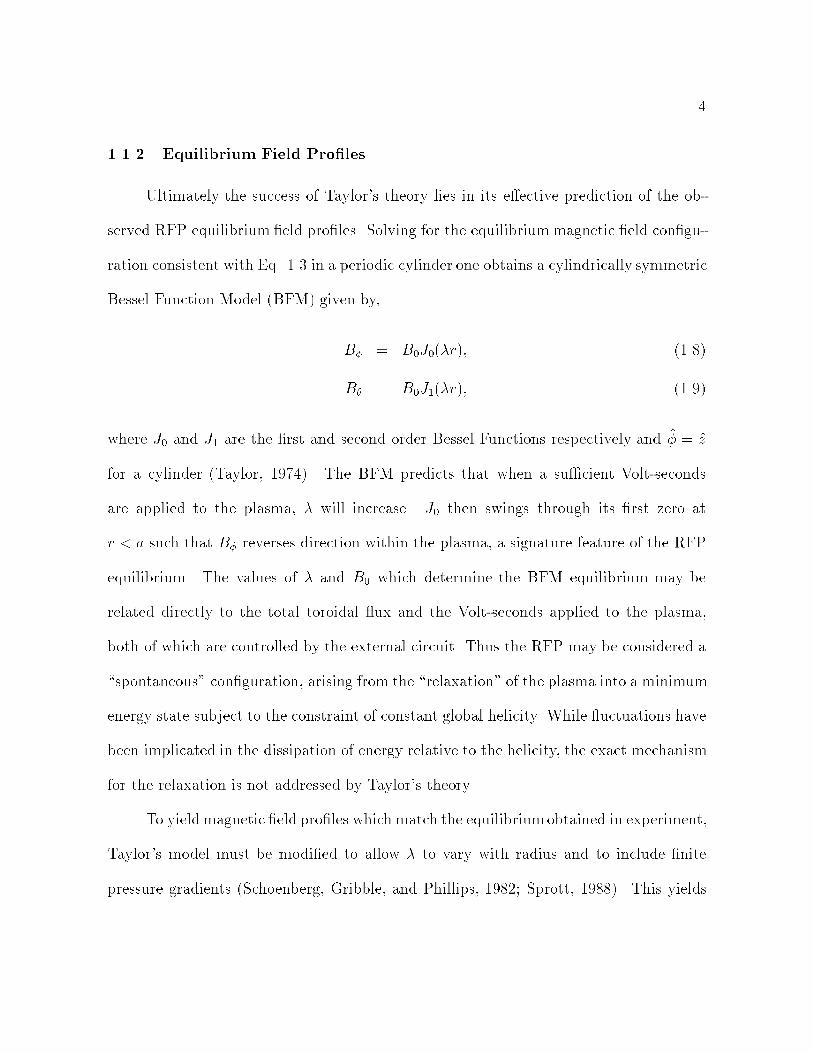
Ultimately the success of Taylor's theory lies in its eective prediction of the ob-

served RFP equilibrium eld proles. Solving for the equilibriummagnetic eld congu-

ration consistent with Eq. 1.3 in a periodic cylinder one obtains a cylindrically symmetric

Bessel Function Model (BFM) given by,

B = B0J0(r); (1.8)

B = B0J1(r); (1.9)

where J0 and J1 are the rst and second order Bessel Functions respectively and = z

for a cylinder (Taylor, 1974). The BFM predicts that when a sucient Volt-seconds

are applied to the plasma, will increase. J0 then swings through its rst zero at

r < a such that B reverses direction within the plasma, a signature feature of the RFP

equilibrium. The values of and B0 which determine the BFM equilibrium may be

related directly to the total toroidal ux and the Volt-seconds applied to the plasma,

both of which are controlled by the external circuit. Thus the RFP may be considered a

\spontaneous" conguration, arising from the \relaxation" of the plasma into a minimum

energy state subject to the constraint of constant global helicity. While uctuations have

been implicated in the dissipation of energy relative to the helicity, the exact mechanism

for the relaxation is not addressed by Taylor's theory.

To yield magnetic eld proles which match the equilibriumobtained in experiment,

Taylor's model must be modied to allow to vary with radius and to include nite

pressure gradients (Schoenberg, Gribble, and Phillips, 1982; Sprott, 1988). This yields

5

r/a

Tesla

0.25

0.20

0.15

0.10

0.05

0.00

-0.05

-0.10

-0.150.0 0.2 0.4 0.6 0.8 1.0

Bφ

Bθ

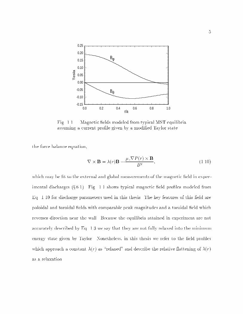
Fig. 1.1.| Magnetic elds modeled from typical MST equilibriaassuming a current prole given by a modied Taylor state.

the force balance equation,

rB = (r)B orP (r)B

B2; (1.10)

which may be t to the external and global measurements of the magnetic eld in exper-

imental discharges (x 6.1). Fig. 1.1 shows typical magnetic eld proles modeled from

Eq. 1.10 for discharge parameters used in this thesis. The key features of this eld are

poloidal and toroidal elds with comparable peak magnitudes and a toroidal eld which

reverses direction near the wall. Because the equilibria attained in experiment are not

accurately described by Eq. 1.3 we say that they are not fully relaxed into the minimum

energy state given by Taylor. Nonetheless, in this thesis we refer to the eld proles

which approach a constant (r) as \relaxed" and describe the relative attening of (r)

as a relaxation.

6

-2.0

-1.5

-1.0

-0.5

0.0

0.5

0.0 0.2 0.4 0.6 0.8 1.0

current over-driven

r/a

Volts/m ηJ||

E||

current under-driven

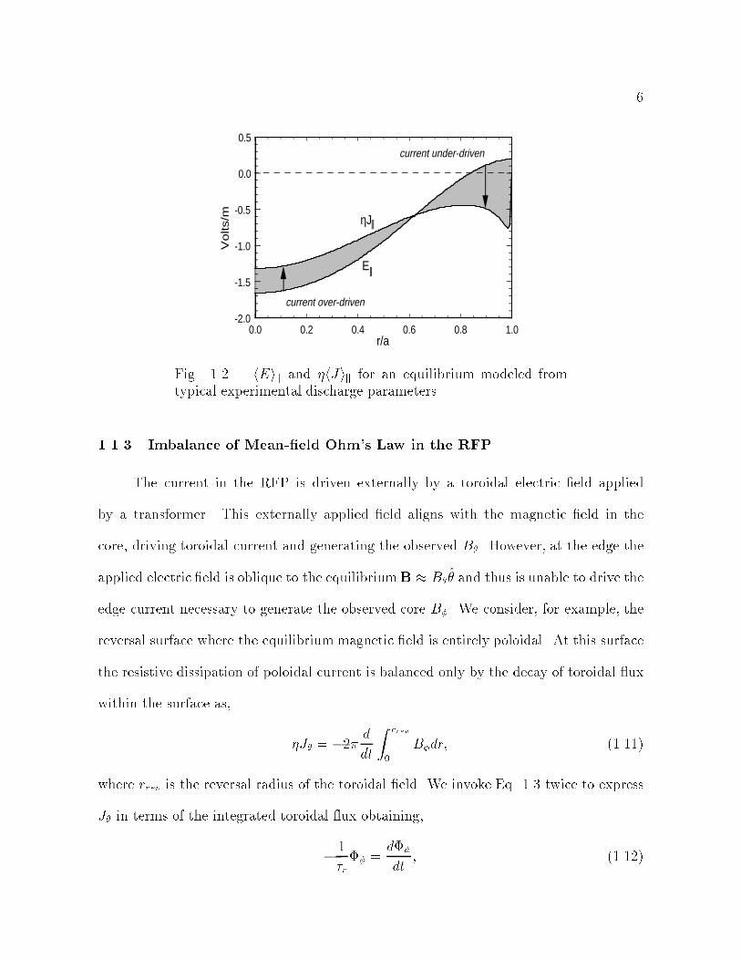
Fig. 1.2.| hEik and hJik for an equilibrium modeled fromtypical experimental discharge parameters.

1.1.3 Imbalance of Mean-eld Ohm's Law in the RFP

The current in the RFP is driven externally by a toroidal electric eld applied

by a transformer. This externally applied eld aligns with the magnetic eld in the

core, driving toroidal current and generating the observed B. However, at the edge the

applied electric eld is oblique to the equilibriumB B and thus is unable to drive the

edge current necessary to generate the observed core B. We consider, for example, the

reversal surface where the equilibrium magnetic eld is entirely poloidal. At this surface

the resistive dissipation of poloidal current is balanced only by the decay of toroidal ux

within the surface as,

J = 2 ddt

Z rrev

0

Bdr; (1.11)

where rrev is the reversal radius of the toroidal eld. We invoke Eq. 1.3 twice to express

J in terms of the integrated toroidal ux obtaining,

1

r =

d

dt; (1.12)

7

where r is a resistive diusion time. However, in experiments this decay is not observed,

rather the toroidal ux is maintained for as long as an electric eld is applied by the

transformer. Thus we presume the existence of an auxiliary current drive mechanism

which drives current in the edge.

To quantify the approximate imbalance in Ohm's Law over the plasma radius we

may overplot hEik and hJik (Fig. 1.2). Using estimated values for we obtain the

expected imbalance at the edge where the applied parallel electric eld is too small or in

the wrong direction to account for the driven current. In addition we obtain an imbalance

in the core where the applied eld over drives the necessary current. Thus, the applied

eld acts to peak the current, pushing the equilibrium away from the constant relaxed

state predicted by Taylor. Clearly, an anomalous drive term is needed to atten the

current prole, suppressing current in the core and driving it in the edge. We must move

beyond Taylor's theory to nd candidates for that term.

1.2 Dynamos

It has been long proposed that the parallel Ohm's law may be balanced in the

RFP by retaining the nonlinear product of uctuations in the ion velocity and magnetic

eld averaged over a ux surface (Eq. 1.1). The nonlinear h~v ~bi term would act to

drive parallel current in the edge and suppress it in the core to maintain a magnetic eld

prole characteristic of the relaxed Taylor state. This generation of magnetic ux from

ow uctuations in a conducting uid is an example of a general class of phenomena

called dynamos. The existence and properties of dynamos have been the subject of

extensive theoretical eorts and numerical studies with interest stemming in large part

from evidence of naturally occurring geophysical and astrophysical dynamos. In this

8

section we begin with a brief description of kinematic dynamo theory which has been

historically employed to describe dynamos occurring in systems dominated by the kinetic

energy of the uid. Extensive monographs exist on this subject including the classic text

by Moat (1978), and the more recent book by Childress (1995). We then outline a

nonlinear theory of the MHD dynamo which is applicable to the strong-eld regime of

the RFP and demonstrate how this theory relates (or fails to relate) to the traditional

kinematic dynamo. We end by mentioning an alternative kinetic theory for the relaxation

of the RFP current prole and discuss the status of that theory in RFP studies.

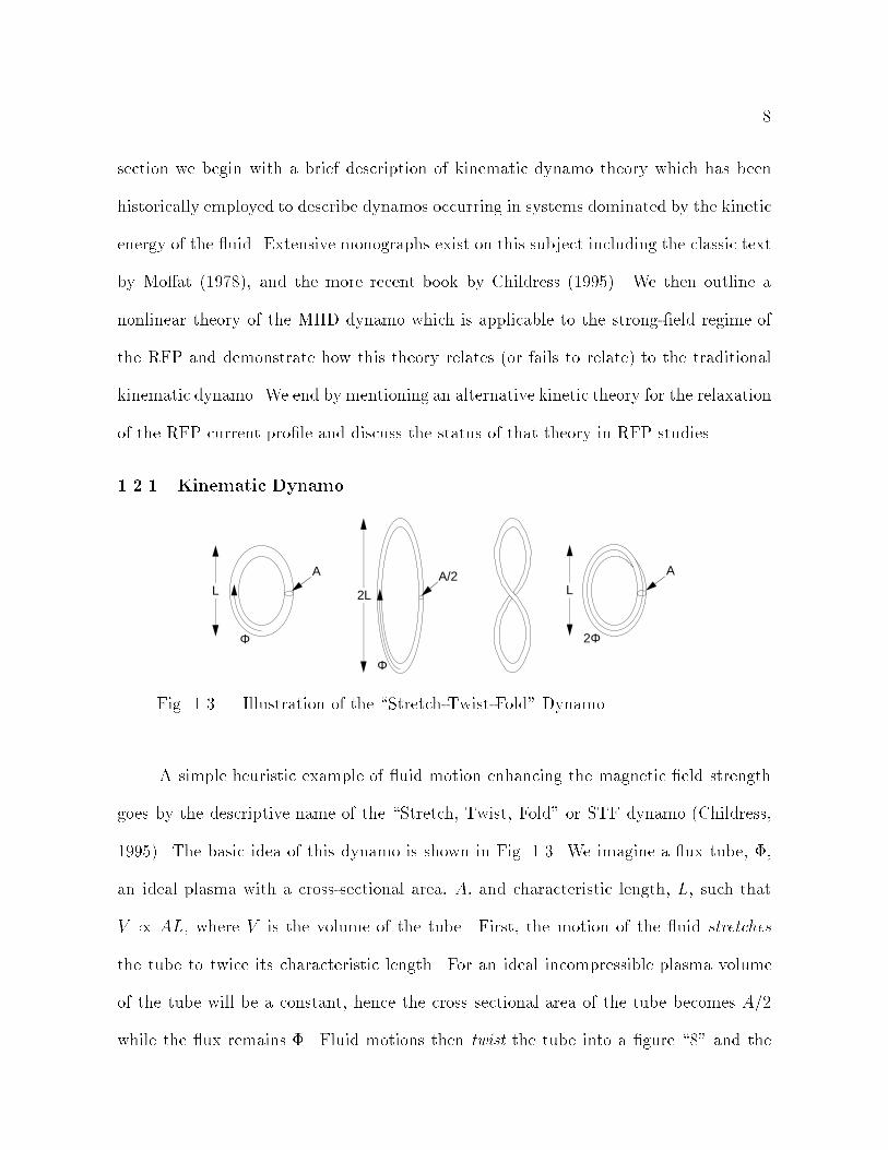
1.2.1 Kinematic Dynamo

A

Φ

L 2L

Φ

A/2 A

L

2Φ

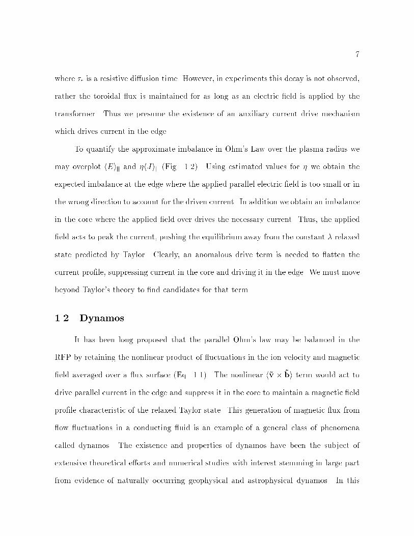
Fig. 1.3.| Illustration of the \Stretch-Twist-Fold" Dynamo.

A simple heuristic example of uid motion enhancing the magnetic eld strength

goes by the descriptive name of the \Stretch, Twist, Fold" or STF dynamo (Childress,

1995). The basic idea of this dynamo is shown in Fig. 1.3. We imagine a ux tube, ,

an ideal plasma with a cross-sectional area, A, and characteristic length, L, such that

V / AL, where V is the volume of the tube. First, the motion of the uid stretches

the tube to twice its characteristic length. For an ideal incompressible plasma volume

of the tube will be a constant, hence the cross sectional area of the tube becomes A=2

while the ux remains . Fluid motions then twist the tube into a gure \8" and the

9

fold two halves over each other such that the loop occupies its original volume. However,

now there is double the ux through A. In principle the STF motion may be repeated

to create an arbitrarily strong ux loop. This assumes that the Lorentz force associated

with the growing eld strength of the loop remain much weaker than the ux enhancing

motion of the conducting medium.

The STF is a simple example of a kinematic dynamo mechanism in which the energy

of the uid motion is assumed to dominate the energy of the growing magnetic eld. A

general approach to the dynamo problem begins with the magnetic induction equation,

@B

@t= rE = r (vB) + r2B; (1.13)

By separating each quantity x into a mean, x0, and uctuating, ~x, such that hxi = x0

and h~xi = 0, we may linearize Eq. 1.13 into its mean and uctuating components,

@B0

@t= r

v0 B0 + h~v ~bi

+ r2B0; (1.14)

@~b

@t= r

~v B0 + v0 ~b

+ r2~b: (1.15)

Kinematic dynamo theory neglects the JB back-reaction of the magnetic eld onto the

uid motion making Eqs. 1.141.15 linear in ~b. One is then free to specify a ~v, solve for

the resulting ~b from Eq. 1.15, and calculate the resulting h~v ~bi to see if it overcomes

the eects of resistive dissipation to generate B0. Such solutions are known to exist and

their properties have been extensively studied.

The statistical properties of ~v in an isotropic, homogenous turbulent mediumwhich

are consistent with h~v~bi > 0 may be determined through expansion of h~v~bi in terms

of the mean eld B0 and its derivatives. This yields the well known result (Moat, 1978;

10

Parker, 1979; Krause and Radler, 1980; Zeldovich et al., 1983),

Ef h~v ~bi = 0B0 0J0: (1.16)

The 0 and 0 coecients are given by the statistical properties of the uid uctuation,

0 = 3h~w ~vi; (1.17)

0 =

3h j~vj2i; (1.18)

where is a typical eddy-turnover time and ~w = r ~v is the uctuating uid vorticity.

Substituting the Ef from Eq. 1.16 back into Eq. 1.14 we obtain,

@B0

@t= r (v0 B0 + 0B0) + ( + 0)r2B0: (1.19)

We see here that the presence of uid uctuations act through 0 to enhance the resistive

dissipation of B0. However, if 0 drives current parallel to the eld with the proper

geometry the uid uctuations may generate B0. The generation of eld through this

term is called the -eect dynamo.

The kinematic description of the dynamo will eventually break down as the mag-

netic energy grows in magnitude relative to the uid energy. Eventually the back-reaction

of the magnetic eld on the uid uctuations must be considered. In the weak magnetic

eld limit these eects are included through the modication (Vainshtein, 1980; Zeldovich

et al., 1983; Gruzinov and Diamond, 1994) of Eq. 1.17 to include the Lorentz force,

= 0 +

3h~j ~bi: (1.20)

When the the h~j ~bi balances the 0 term the dynamo is said to have saturated. The

behavior of these saturated dynamos is a topic of both considerable interest and debate

11

as the dynamos which may exist in astrophysical or geophysical systems are presumed to

exist in this state. Recent numerical work (e.g. Cattaneo and Hughes, 1996) suggests that

the behavior of dynamos in these saturated regimes diers qualitatively from what might

be extrapolated from the kinematic growth phase. Furthermore, as we discuss below, in

the strong-eld limit applicable to laboratory plasmas the kinematic description breaks

down altogether and a physically distinct dynamo mechanism emerges.

1.2.2 MHD Dynamo

The RFP plasma exists in a strong magnetic eld regime for which the kinematic

description fails to apply. In this limit the uid velocity and magnetic eld uctuations

are inextricably linked such that the magnetic induction equation cannot be linearized.

To understand the dynamo in this strong eld limit we may start with the generalized

Ohm's law which includes the JB Lorentz force (Spitzer, 1962),

me

e2ne

@J

@t+E+ vB 1

eneJB+

rPeene

= J; (1.21)

where me and e are the electron mass and charge respectively, ne is the electron density,

and Pe is the electron pressure. We may take the parallel component of Eq. 1.21 averaged

over a ux surface obtaining (Ji, et. al., 1995),

Jk;0 Ek;0 = h~v ~bik 1

eneh~j ~bik

= h(~v ~j=ene) ~bik

h~ve? ~b?ik (1.22)

where we have neglected parallel uctuations in pressure and current and made use of

J = ene(vi ve) and the approximation v vi. To determine the contributions to ~ve?

12

we may take the perpendicular component of Eq. 1.21 yielding,

~ve? = ~v? ~j?=ene

=~E? B

B2+r?

~Pe B

eneB2 me

e2ne

@~j?@t

+ ~j?

!B=B2: (1.23)

We expect the electron inertial and uctuating Hall term to be negligible. This leaves a

single uid MHD contribution in the form of a uctuating ~E? B0 uid velocity, and

a diamagnetic contribution from the uctuating electron pressure gradient. The MHD

contribution to ~ve will appear identically in ~vi which was measured in the work described

in this thesis. By substituting our expression for ~ve into Eq. 1.22 we obtain the following

form for parallel Ohm's law,

Jk;0 Ek;0 = h~E? ~b?i=B0 + hr?~Pe ~b?i=B0ene: (1.24)

In this expression the uctuating velocity is eliminated altogether and the dynamo is

expressed entirely as a product of the uctuating magnetic eld with uctuating electric

eld and electron pressure terms.

To compare this dynamo mechanism to the kinematic dynamo we examine a more

general expression for the -coecient derived by Bhattacharjee and Yuan (1995) for the

MHD dynamo,

=0 + (=3)(J0 B0 + h~E ~bi)

1 + (=3)B2; (1.25)

where 0 is the kinematic -coecient. In the weak eld limit this reduces to 0

recovering the kinematic expression. However, in the strong eld (or high conductivity)

limit, (=3)B20 1 this reduces to,

(J0 B0 + h~E ~bi)=B2; (1.26)

13

We may substitute this expression back into Eq. 1.16 to obtain the strong eld expression

for the uctuation induced electric eld,

h~v ~bi =J0 B0 + h~E ~bi

B0=B

2 J0

= J0;? + h~E ~biB0=B2: (1.27)

Taking the parallel component of this expression we obtain,

h~v ~bik = h~E ~bi=B; (1.28)

This matches the MHD term derived above from the generalized Ohm's law. Thus

the dynamo mechanism in the strong eld limit of the RFP is a completely distinct

mechanism from that responsible for the kinematic dynamo. This is brought about by

the domination of 0 by the MHD terms in the numerator of Eq. 1.25 and the subsequent

cancellation of the parallel -eect with the remaining, non-MHD term in the numerator.

1.2.3 Kinetic Dynamo

A completely dierent mechanism for the attening of the current prole has been

proposed by Jacobson and Moses (1984). It is known that the large magnetic uctuations

and overlapping island structure in the RFP induce stochasticity in the mean magnetic

eld such that a eld line followed about the machine will wander randomly in radius.

This eld line wander yields high particle and energy diusivity (Rechester and Rosen-

bluth, 1978) as hot core particles stream rapidly parallel to the stochastic elds out of

the plasma. This eld line diusion is predicted to exceed the diusion of the particles

due to classical collisional cross-eld transport. Jacobson and Moses propose that par-

allel electron momentum driven by the applied electric eld in the core streams along

the magnetic eld to the edge region where the eld is predominantly poloidal. Such

14

a mechanism would act to atten the parallel current prole in accordance to Taylor's

theory without a h~v ~bi dynamo mechanism.

Recent Fokker-Plank simulation of electron distributions in the RFP with a paral-

lel momentum diusion set to be consistent with Rechester-Rosenbluth diusivity sug-

gest that the kinetic dynamo mechanism could produce the observed RFP equilibrium

(Giruzzi and Martines, 1994; Martines and Vallone, 1997). However, a self-consistent

theoretical treatment of the problem by Terry and Diamond (1990) indicated electron

diusion rates far below those needed to explain the observed attening of the current

prole. Furthermore, experimental measurements of the electron momentumdistribution

at the edge of MST do not appear to be consistent with the streaming of fast electrons

from the core to the edge (Stoneking, PhD Thesis, 1994). While measurements described

below and the results reported in this thesis provide strong evidence for MHD dynamo

activity in the edge and core region of the MST, detailed commentary on the validity of

the kinetic dynamo for the MST falls outside the scope of the present work.

1.3 Evidence for the MHD Dynamo in the RFP

1.3.1 MHD Simulation

The inherently nonlinear nature of the dynamo in the RFP make computational

eorts to simulate dynamo eects invaluable. The original numerical simulations of the

RFP performed by Sykes and Wesson (1977) employed a periodic 14 14 13 grid and

exhibited strong dynamo activity. Since that time extensive numerical eorts have been

devoted to simulation of dynamics in the RFP. For a thorough review of these eorts

the reader is again referred to Ortlani and Schnack (1993). These simulations have con-

15

sistently demonstrated relaxation of the current prole by a dynamo electric eld with

the RFP equilibrium maintained indenitely with a constant applied electric eld. The

dynamo eld was observed in linear codes which contained only m=1 resonant modes,

while in fully developed nonlinear codes the m = 1 contribution still dominated. The

inclusion of multiple modes did aect the dynamics of the observed equilibrium with

oscillations in the current prole becoming evident. Such eects were more pronounced

as the simulations approached Lundquist number regimes similar to those achieved in ex-

periment, with the oscillations approaching the discrete relaxation phenomena observed

in experiment. Recent work has employed these simulations to predict low uctuation

regimes which have then been realized in experiment (Sovinec, 1995). Thus far, the nu-

merical work has successfully demonstrated the consistency of the RFP dynamo within

the framework of resistive MHD and demonstrated the orgin and characteristics of the

uctuations observed in the RFP. As these simulations continue to approach experimen-

tal regimes with advances in algorithms and computational resolution, we expect an

increasingly detailed and realistic picture of the dynamo action in the RFP to emerge.

1.3.2 Edge Measurements

Recent experiments by Ji, et.al. (1995) have successfully observed the dynamo in

the edge of several RFP's. These experiments employed a complex Langumiur probe to

measure ~E?, r?~Pe and ~b?. Calculating h~E? ~b?i and hr?

~Pe ~b?i over an ensemble of

discrete dynamo events, Ji demonstrated the balance of Eq. 1.24. In relatively collision-

less plasmas like those obtained in MST it was found that the h~E? ~b?i term dominated

the dynamo contribution while the diamagnetic term was found to dominate for the

higher collisionality plasmas in the TPE-1RM20 device. Edge measurements continue to

16

constrain the edge dynamo on MST. However, measurement of dynamo activity in the

core has required the development of non-perturbing techniques like those described in

this thesis.

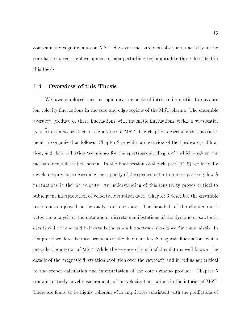
1.4 Overview of this Thesis

We have employed spectroscopic measurements of intrinsic impurities to measure

ion velocity uctuations in the core and edge regions of the MST plasma. The ensemble

averaged product of these uctuations with magnetic uctuations yields a substantial

h~v ~bi dynamo product in the interior of MST. The chapters describing this measure-

ment are organized as follows. Chapter 2 provides an overview of the hardware, calibra-

tion, and data reduction techniques for the spectroscopic diagnostic which enabled the

measurements described herein. In the nal section of the chapter (x 2.5) we formally

develop expressions describing the capacity of the spectrometer to resolve passively low-k

uctuations in the ion velocity. An understanding of this sensitivity proves critical to

subsequent interpretation of velocity uctuation data. Chapter 3 describes the ensemble

techniques employed in the analysis of our data. The rst half of the chapter moti-

vates the analysis of the data about discrete manifestations of the dynamo or sawtooth

events while the second half details the ensemble software developed for the analysis. In

Chapter 4 we describe measurements of the dominant low-k magnetic uctuations which

pervade the interior of MST. While the essence of much of this data is well known, the

details of the magnetic uctuation evolution over the sawtooth and in radius are critical

to the proper calculation and interpretation of the core dynamo product. Chapter 5

contains entirely novel measurements of ion velocity uctuations in the interior of MST.

These are found to be highly coherent with amplitudes consistent with the predictions of

17

MHD. In addition the radial uctuation prole of the ion velocity uctuations is found to

be signicantly limited in contrast to the extended prole of the magnetic uctuations.

Chapter 6 consists of two parts. The rst part details dynamic modeling of the RFP

equilibrium quantities in an eort to predict the magnitude and direction of the dynamo

eld necessary to balance Ohm's law. The second part presents the measured dynamo

products in the interior of the plasma and compares them to the predictions of the mod-

eling. The observations reported here of substantial dynamo eld in the core, peaking to

several Volts/m at the sawtooth crash, constitute the central result of this thesis. How-

ever, comparison with predictions of the model suggests that substantial improvements

in measurement and modeling techniques are needed to demonstrate numerical balance

of Eq. 1.1 in the interior of MST.

References

Bhattacharjee, A. and E. Hameiri (1986). Self-consistent dynamolike activity in turbulentplasmas. Phys. Rev. Lett. 57(2), 206209.

Bhattacharjee, A. and Y. Yuan (1995). Self-consistency constraints on the dynamo mech-anism. ApJ 449, 739744.

Boozer, A. H. (1986). Phys. Fluids 29, 4123.

Cattaneo, F. and D. W. Hughes (1996). Nonlinear saturation of the turbulent eect.Phys. Rev. E 54(5), R4532R4535.

Childress, S. and A. D. Gilbert (1995). Stretch, twist, fold : the fast dynamo. New York:Springer.

Giruzzi, G. and E. Martines (1994). Kinetic modeling of fast electron dynamics and self-consistent magnetic elds in a reversed eld pinch. Phys. Plasmas 1(8), 26532660.

Gruzinov, A. V. and P. H. Diamond (1994). Phys. Rev. Lett. 72, 1651.

Jacobson, A. R. and R. W. Moses (1984). Nonlocal dc electrical conductivity of a lorentzplasma in a stochastic magneic eld. Phys. Rev. A 29(6), 33353342.

18

Ji, H., A. F. Almagri, S. C. Prager, and J. S. Sar (1995). Measurement of the dynamoeect in a plasma. Phys. Plasmas 3(5), 19351942.

Ji, H., S. C. Prager, and J. S. Sar (1995). Conservation of magnetic helicity duringplasma relaxation. Phys. Rev. Lett. 74(15), 29452948.

Krause, F. and K.-H. Radler (1980). Mean-Field Magnetohydrodynamics and DynamoTheory. Oxford: Pergamon.

Martines, E. and F. Vallone (1997). Ohm's law for plasmas in reversed eld pinchconguration. Phys. Rev. E 56(1), 957962.

Moat, H. K. (1978). Magnetic Field Generation in Electrically Conducting Fluids.Cambridge, U. K.: Cambridge U. P.

Ortlani, S. and D. D. Schnack (1993). Magnetohydrodynamics of Plasma Relaxation.Singapore: World Scientic.

Parker, E. N. (1979). Cosmic Magnetic Fieds, Their Orgin and Activity. Oxford: Claren-don.

Rechester, A. B. and M. N. Rosenbluth (1978). Electron heat transport in a tokamakwith destroyed magnetic surfaces. Phys. Rev. Lett. 40(1), 3841.

Schoenberg, K. F., R. F. Gribble, and J. A. Phillips (1982). Zero-dimensional simulationsof reversed-eld pinch experiments. Nuclear Fusion 22(11), 14331441.

Sovinec, C. R. (1995). Magnetohydrodynamic simulations of noninductive helicity in-jection in the reversed-eld pinch and tokamak. PhD dissertation, University ofWisconsin Madison, Department of Physics.

Spitzer, Jr., L. (1962). Physics of Fully Ionized Gases. New York: Interscience Publishers.

Sprott, J. C. (1988). Electrical circuit modeling of reversed eld pinches. Phys. Flu-ids 31(8), 22662275.

Stoneking, M. R. (1993). Fast electron generation and transport in a turbulent magnetizedplasma. PhD dissertation, University of Wisconsin Madison, Department ofPhysics.

Sykes, A. and J. A. Wesson (1977). Proc. 8th European Conf. on Cont. Fusion andPlasma Physics, Prague, pp. 80. Czechoslavak Acadamy of Sciences.

Taylor, J. B. (1974). Relaxation of toroidal plasma and generation of reverse magneticelds. Phys. Rev. Lett. 33(19), 11391141.

Terry, P. W. and P. H. Diamond (1990). A self-consistent theory of radial transport ofeld-aligned current by microturbulence. Phys. Fluids B 2(6), 11281137.

Vainshtein, S. I. (1980). Magnetohydrodynamics 16, 111.

Zeldovich, Y. B., A. A. Ruzmaikin, and D. D. Sokolo (1983). Magnetic Fields inAstrophysics. New York: Gordon & Breach.

19

2

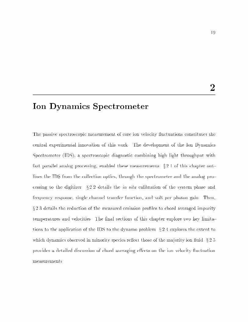
Ion Dynamics Spectrometer

The passive spectroscopic measurement of core ion velocity uctuations constitutes the

central experimental innovation of this work. The development of the Ion Dynamics

Spectrometer (IDS), a spectroscopic diagnostic combining high light throughput with

fast parallel analog processing, enabled these measurements. x 2.1 of this chapter out-

lines the IDS from the collection optics, through the spectrometer and the analog pro-

cessing to the digitizer. x 2.2 details the in situ calibration of the system phase and

frequency response, single channel transfer function, and volt per photon gain. Then,

x 2.3 details the reduction of the measured emission proles to chord averaged impurity

temperatures and velocities. The nal sections of this chapter explore two key limita-

tions to the application of the IDS to the dynamo problem. x 2.4 explores the extent to

which dynamics observed in minority species re ect those of the majority ion uid. x 2.5

provides a detailed discussion of chord averaging eects on the ion velocity uctuation

measurements.

20

FocusingMirror

Exit Plane

Cze

rny-

Tur

ner

Duo

-Spe

ctro

met

er

F.O. Bundles

PMT Array

Entrance Slit

Grating

Bulk Ion Flow

Mirror

MST Vacuum Vessel

Lens4.5'' Port

Filter Monochrometer

Fiber OpticBundles

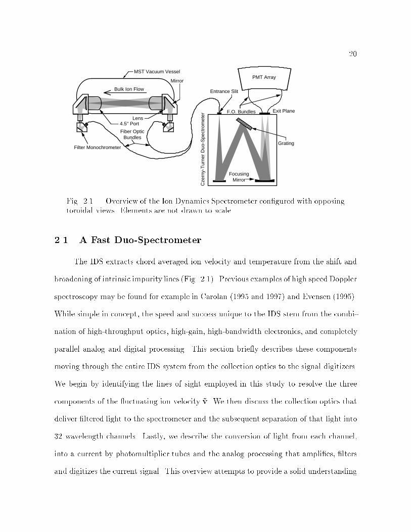
Fig. 2.1.| Overview of the Ion Dynamics Spectrometer congured with opposingtoroidal views. Elements are not drawn to scale.

2.1 A Fast Duo-Spectrometer

The IDS extracts chord averaged ion velocity and temperature from the shift and

broadening of intrinsic impurity lines (Fig. 2.1). Previous examples of high speed Doppler

spectroscopy may be found for example in Carolan (1995 and 1997) and Evensen (1995).

While simple in concept, the speed and success unique to the IDS stem from the combi-

nation of high-throughput optics, high-gain, high-bandwidth electronics, and completely

parallel analog and digital processing. This section brie y describes these components

moving through the entire IDS system from the collection optics to the signal digitizers.

We begin by identifying the lines of sight employed in this study to resolve the three

components of the uctuating ion velocity ~v. We then discuss the collection optics that

deliver ltered light to the spectrometer and the subsequent separation of that light into

32 wavelength channels. Lastly, we describe the conversion of light from each channel,

into a current by photomultiplier tubes and the analog processing that amplies, lters

and digitizes the current signal. This overview attempts to provide a solid understanding

21

222T138T

0P

-19P

+19P

Fig. 2.2.| Toroidal line of sight. Opposing and up-downsymmetric views shown.

of the IDS system while omitting many of the technical details. Subsequent sections

address some of these details which are specically relevant to this thesis while design

specications may be found in (Den Hartog and Fonck, 1994).

2.1.1 Lines of Sight

The IDS collects light along two lines of sight oriented to maximize sensitivity to

particular components of ~v. The mean toroidal velocity v is measured through the 412

inch ports at poloidal and toroidal angles of -19P, 138T and -19P, 222T, by opposing

the two views along the same toroidal chord.1 This chord (shown to scale in Fig. 2.2)

subtends a toroidal angle of 84o about 180T, approximately 17 cm (0:33 a) below the

midplane of the torus. The midpoint of the chord falls almost directly below the major

radius of the torus yielding a radial impact parameter for the chord roughly equal to

its vertical displacement from the midplane. By employing the opposing views we may

1Throughout this thesis the convention |P, |T will be used to indicate poloidal and toroidal anglesof ports and diagnostics in machine coordinates measured relative to the poloidal and toroidal gaps inthe shell.

22

to compare red shifted and blue shifted emission lines to obtain an absolute measure-

ment of the ion velocity. Alternatively, the views may provide an in situ calibration

of the unshifted line position, allowing subsequent measurements of ion velocity with

non-opposing views (x 2.3). Measurements of toroidal velocity uctuation, ~v require no

calibration of the mean ow making the two chords redundant. For ~v measurements

we look through the 412inch ports at -19P, 222T and +19P, 222T along toroidal chords

which mirror each other about the midplane. The up-down symmetry of this congura-

tion allows the extraction of the local velocity uctuation phase from the chord averaged

quantity (x 2.5). Most ~v measurements reported in this study employed the up-down

toroidal conguration.

-22.5P

0.62

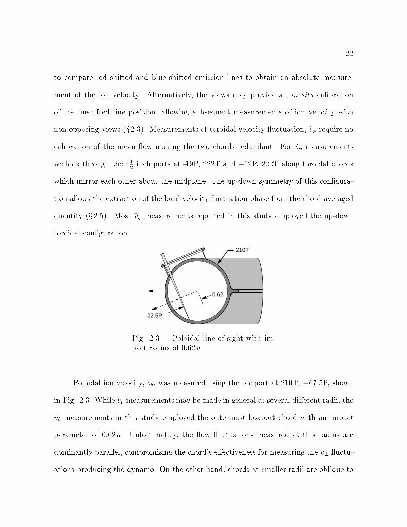
210T

Fig. 2.3.| Poloidal line of sight with im-pact radius of 0:62 a

Poloidal ion velocity, v, was measured using the boxport at 210T, +67.5P, shown

in Fig. 2.3. While v measurements may be made in general at several dierent radii, the

~v measurements in this study employed the outermost boxport chord with an impact

parameter of 0:62 a. Unfortunately, the ow uctuations measured at this radius are

dominantly parallel, compromising the chord's eectiveness for measuring the v? uctu-

ations producing the dynamo. On the other hand, chords at smaller radii are oblique to

23

except near the core making any resolution of v dicult. We explore this issue further

in our discussion of the ~v measurement results.

138T

+19P

Fig. 2.4.| Radial line of sight.

Radial ows were measured through the 412 inch port at 138T, +19P along a line

of sight passing through the center of the torus (Fig. 2.4). While mean radial ows

cancel out from one half of the chord to the other, radial uctuations with poloidal mode

number m = 1, which \turn around" as they reach the second half of the chord, are

resolved perfectly. This, combined with a direct view through the large port provided a

near optimal measurement of radial velocity uctuations, ~vr.

2.1.2 Optics

UV-grade fused silica lenses collect the radiation from each chord. For the toroidal

views 4 inch lenses look through 412inch ports with their aperture constricted by an

oblique viewing angle and the 5 cm thick vessel wall. The lenses focus onto the face of the

opposing lens in order to reduce the collection of re ected light. This produces a conical

collection volume that, according to etendue calculations and ray tracing simulations,

collects light from an extended plasma volume with uniform optical weighting along the

line of sight. The poloidal view looks directly through a 112 inch aperture with a 2 inch

lens. Likewise, the radial view looks directly through a 412inch aperture with an large

24

7inch

lens.

For

thetoroid

alandpoloid

alview

sthelen

sform

sthevacu

um

sealfor

the

system

while

therad

ialview

looksthrou

ghalarge

fused

silicawindow

which

formsthe

seal.Ligh

tcollected

bythelen

sfocu

seson

theentran

ceslit

ofsm

allmonoch

romators

that

lter

brigh

toutly

inglines

capableofcon

taminatin

gtheselected

emission

line.The

width

ofthemonoch

romator

transfer

function

greatlyexceed

stheim

purity

linewidth

andthusdoes

not

alterthewavelen

gthdistrib

ution

oftheem

ittedrad

iation.

Ch. 1-16

Ch. 17-32

entrance slit

exit plane

exit image

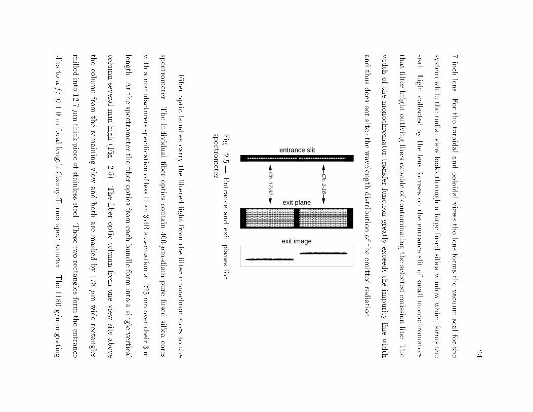
Fig.

2.5.|Entran

ceandexitplan

esfor

spectrom

eter.

Fiber

optic

bundles

carrytheltered

lightfrom

thelter

monoch

romators

tothe

spectrom

eter.Theindividual

ber

optics

contain

400-m-diam

pure

fused

silicacores

with

amanufactu

rersspeci

cationofless

than

3dBatten

uation

at225

nmover

their

3m

length

.Atthespectrom

etertheber

optics

fromeach

bundleform

into

asin

glevertical

columnseveral

mm

high

(Fig.

2.5).Theber

optic

columnfrom

oneview

sitsabove

thecolu

mnfrom

therem

ainingview

andboth

aremasked

by178

m

widerectan

gles

milled

into

12.7mthick

piece

ofstain

lesssteel.

These

tworectan

glesform

theentran

ce

slitsto

af/10

1.0m

focallen

gthCzern

y-Turner

spectrom

eter.The1180

g/mm

grating

25

110001011000101100011001101001110100010001000001010101011101010110100010110011010101110010110101011110101

+

- +

-

+

-

PMT

I-V Pre-Amp

Four-Pole Chebychev Filter

Buffer Amplifer

1 MHzDigitizer

1100 V1000 V

900 V

High VoltagePower Supply

IDS

Fig. 2.6.| Cartoon of analog processing for a single IDS channel.

of the spectrometer yields a reciprocal dispersion of 0.12 nm/mm in fth order at 227

nm. Two sets of 16 tightly packed ber optic columns form the spectrometer exit plane.

The ber optics in each column contain 200-m-diam pure fused silica cores yielding

single ber transfer functions approximately 0.024 nm wide. Each column then forms

into a single ber optic bundle carrying the light for that wavelength channel a nal

0.5 m to a photomultiplier tube. Before reaching the exit plane light from each view is

processed almost identically along parallel optical paths. Now leaving the exit plane the

light from each view separates into 16 overlapping wavelength channels to be processed

subsequently along a total of 32 nearly identical analog paths.

26

2.1.3 Electronics

The analog processing components for a single IDS channel are shown schematically

in Fig. 2.6. The light for each channel leaves the exit plane ber optic bundle in an f / 10

cone before striking a fused silica window photomultiplier tube (PMT) which converts

each photon into a cascade of photoelectrons. Calibrations presented in the following

section indicate that for typical plasmas, the PMTs typically operate in counting mode,

meaning simply that the cascade from one incident photon usually ceases before the next

begins. The PMT power supply is typically set to 900 Volts for bright dirty plasmas

to 1100 Volts for clean plasmas with little impurity radiation. Individual PMTs biases

are set by voltage dividers to roughly half that value. While the PMTs may in principle

withstand higher biasing voltages the underlying lack of photon statistics in such cases

makes amplication of the individual photoelectron pulses pointless. Current pulses from

the PMT enter directly into high-gain I/V ampliers. These ampliers contain two very

fast operational ampliers operated in series to convert the small current pulses into

measurable signals of several Volts. This voltage travels via BNC cable to a four-pole,

low-pass Chebychev lter with a relatively at response out to 250 kHz. The ltered

signal passes through a unity gain buer amplier to an Aurora 14 digitizer that digitizes

the signal with 12-bit resolution at 1 Mhz.

2.2 Calibration

Three calibrations quantied the performance characteristics of the IDS system.

First, an in situ calibration of the system phase and frequency response demonstrated

the wide bandwidth, non-dispersive character of the analog processing. Second, position,

transfer function, and gain of each channel was swept out by a Cd II line, provided by

27

a Cadmium lamp. This revealed overlapping triangular transfer functions with 0.24 A

FWHM in fth order, meeting the design specications. Finally, illumination with an

integrating sphere of known intensity provided estimates of the system's Volt per pho-

ton gain and overall optical eciency. These estimates indicate that while sensitive and

ecient, the IDS operates in a regime dominated by photon noise, producing inherently

noisy signals which may be improved only at the expense of time resolution. This sec-

tion provides details of the calibration procedure and results in a condensed version of

(Chapman and Den Hartog, 1996).

2.2.1 Phase and Amplitude Response

QuatechWSB-100

Ion Dynam

ics Spectrom

eter

PMT's

Amplifiers

Filters

Czerny-TurnerTTL ÷20

Aurora 14Digitizers

SIGX32REFCLK

32 Channels

Ion DynamicsSpectrometer

in situPhase Calibration

F.O.10

1K9

Fig. 2.7.| Schematic of the in situ calibration of theIDS response amplitude and phase. The Quatech WSB-100 provides the clock for both the driving signal and theAurora 14 digitizers.

We performed a highly resolved in situ calibration of the entire IDS system phase

response from 5 to 500 kHz (Fig. 2.7). The Quatech WSB-100 programmable D/A

board, the key component of the calibration, generates an arbitrary function with 12 bit

vertical resolution and a 20 MHz clock rate. The signal generator drove a bright LED

producing an oscillating light signal that the ber optics collected and passed through

28

the full IDS system.

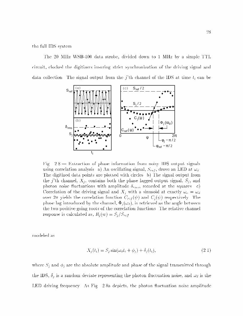
The 20 MHz WSB-100 data strobe, divided down to 1 MHz by a simple TTL

circuit, clocked the digitizers insuring strict synchronization of the driving signal and

data collection. The signal output from the j'th channel of the IDS at time ti can be

δ rms

Sj

Sref

(b)

(a)

Φ j (ωd )

(c)

Cref ( ψ)

C j(ψ )

Sref / 2

Sj / 2

ψ

φref − π/ 2

φj − π / 20 2π

ti

Fig. 2.8.| Extraction of phase information from noisy IDS output signalsusing correlation analysis. a) An oscillating signal, Sref , drove an LED at !d.The digitized data points are plotted with circles. b) The signal output fromthe j'th channel, Xj , contains both the phase lagged output signal, Sj , andphoton noise uctuations with amplitude rms, recorded at the squares. c)Correlation of the driving signal and Xj with a sinusoid at exactly !o = !dover 2 yields the correlation function Cref ( ) and Cj( ) respectively. Thephase lag introduced by the channel, j(!d), is retrieved as the angle betweenthe two positive going roots of the correlation functions. The relative channelresponse is calculated as, Rj(w) = Sj=Sref .

modeled as

Xj(ti) = Sj sin(!dti + j) + j(ti); (2.1)

where Sj and j are the absolute amplitude and phase of the signal transmitted through

the IDS, j is a random deviate representing the photon uctuation noise, and !d is the

LED driving frequency. As Fig. 2.8a depicts, the photon uctuation noise amplitude

29

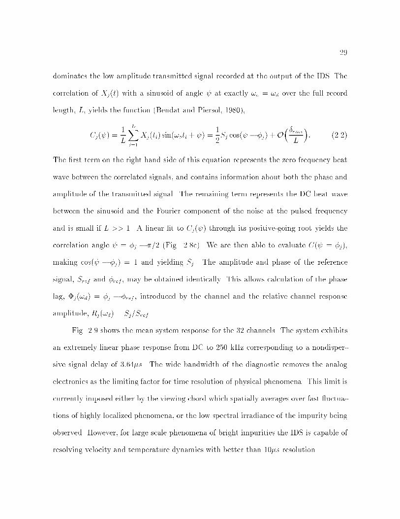
dominates the low amplitude transmitted signal recorded at the output of the IDS. The

correlation of Xj(t) with a sinusoid of angle at exactly !o = !d over the full record

length, L, yields the function (Bendat and Piersol, 1980),

Cj( ) =1

L

LXi=1

Xj(ti) sin(!oti + ) =1

2Sj cos( j) +O

rms

L

: (2.2)

The rst term on the right hand side of this equation represents the zero frequency beat

wave between the correlated signals, and contains information about both the phase and

amplitude of the transmitted signal. The remaining term represents the DC beat wave

between the sinusoid and the Fourier component of the noise at the pulsed frequency

and is small if L >> 1. A linear t to Cj( ) through its positive-going root yields the

correlation angle = j =2 (Fig. 2.8c). We are then able to evaluate C( = j),

making cos( j) = 1 and yielding Sj . The amplitude and phase of the reference

signal, Sref and ref , may be obtained identically. This allows calculation of the phase

lag, j(!d) = j ref , introduced by the channel and the relative channel response

amplitude, Rj(!d) = Sj=Sref .

Fig. 2.9 shows the mean system response for the 32 channels. The system exhibits

an extremely linear phase response from DC to 250 kHz corresponding to a nondisper-

sive signal delay of 3:64s. The wide bandwidth of the diagnostic removes the analog

electronics as the limiting factor for time resolution of physical phenomena. This limit is

currently imposed either by the viewing chord which spatially averages over fast uctua-

tions of highly localized phenomena, or the low spectral irradiance of the impurity being

observed. However, for large scale phenomena of bright impurities the IDS is capable of

resolving velocity and temperature dynamics with better than 10s resolution.

30

0 100 200 300 400 500

0

-π

-2π

-3π

frequency (kHz)

Φ(ω

) (r

ad)

0

-5

-10

-15

-20

-25

R(ω

) (dB)

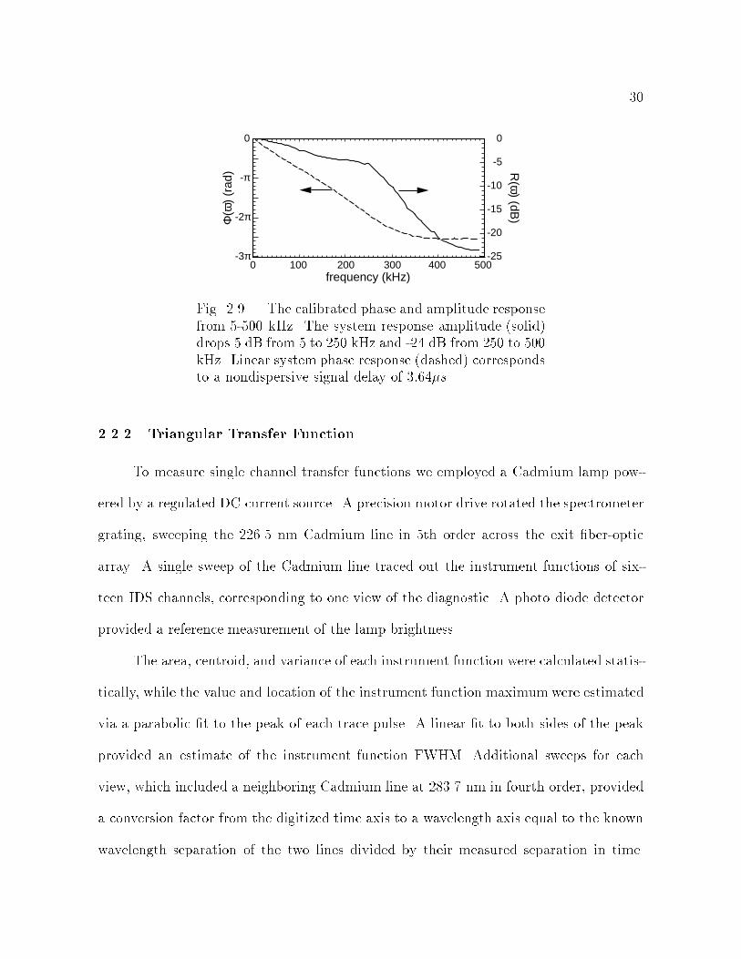
Fig. 2.9.| The calibrated phase and amplitude responsefrom 5-500 kHz. The system response amplitude (solid)drops 5 dB from 5 to 250 kHz and -24 dB from 250 to 500kHz. Linear system phase response (dashed) correspondsto a nondispersive signal delay of 3:64s.

2.2.2 Triangular Transfer Function

To measure single channel transfer functions we employed a Cadmium lamp pow-

ered by a regulated DC current source. A precision motor drive rotated the spectrometer

grating, sweeping the 226.5 nm Cadmium line in 5th order across the exit ber-optic

array. A single sweep of the Cadmium line traced out the instrument functions of six-

teen IDS channels, corresponding to one view of the diagnostic. A photo diode detector

provided a reference measurement of the lamp brightness.

The area, centroid, and variance of each instrument function were calculated statis-

tically, while the value and location of the instrument function maximumwere estimated

via a parabolic t to the peak of each trace pulse. A linear t to both sides of the peak

provided an estimate of the instrument function FWHM. Additional sweeps for each

view, which included a neighboring Cadmium line at 283.7 nm in fourth order, provided

a conversion factor from the digitized time axis to a wavelength axis equal to the known

wavelength separation of the two lines divided by their measured separation in time.

31

sweep time (seconds)

position (Angstroms)

measured intensity (V

olts)norm

aliz

ed in

tens

ity (

a.u.

)

2.2 1.41.61.82.02.0

1.5

1.0

0.5

0.08580757065

0.0

0.2

0.4

0.6

0.8

1.0

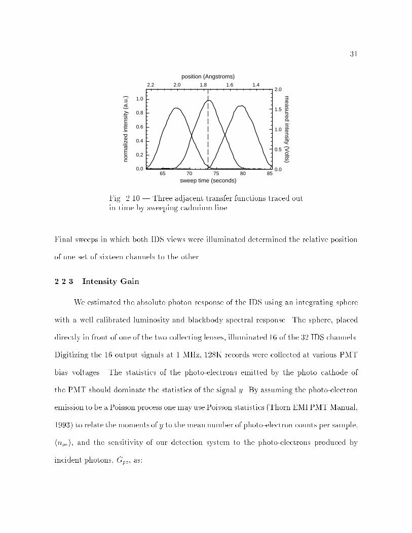
Fig. 2.10.| Three adjacent transfer functions traced outin time by sweeping cadmium line.

Final sweeps in which both IDS views were illuminated determined the relative position

of one set of sixteen channels to the other.

2.2.3 Intensity Gain

We estimated the absolute photon response of the IDS using an integrating sphere

with a well calibrated luminosity and blackbody spectral response. The sphere, placed

directly in front of one of the two collecting lenses, illuminated 16 of the 32 IDS channels.

Digitizing the 16 output signals at 1 MHz, 128K records were collected at various PMT

bias voltages. The statistics of the photo-electrons emitted by the photo cathode of

the PMT should dominate the statistics of the signal y. By assuming the photo-electron

emission to be a Poisson process one may use Poisson statistics (Thorn EMI PMTManual,

1993) to relate the moments of y to the mean number of photo-electron counts per sample,

hnpei, and the sensitivity of our detection system to the photo-electrons produced by

incident photons, Gpe, as:

32

42005

1015

2025

30channel num

ber

position (Angstroms)

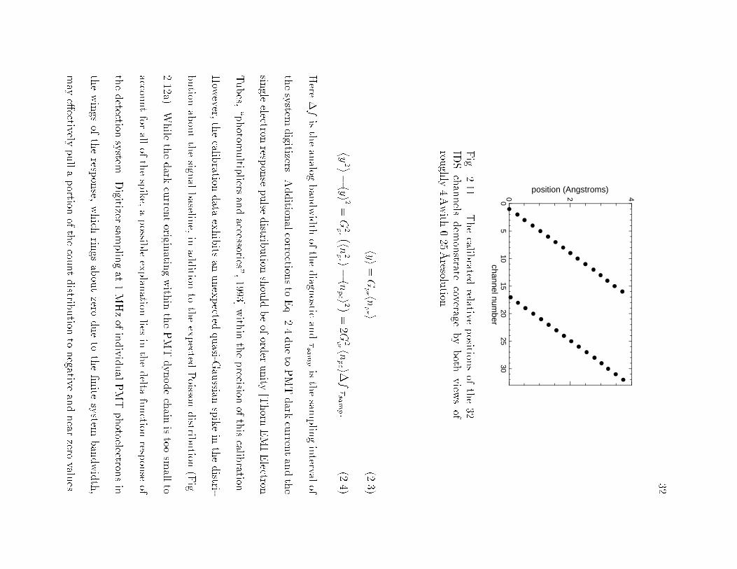
Fig.

2.11.|Thecalib

ratedrelativ

eposition

sof

the32

IDSchannels

dem

onstrate

coveragebyboth

view

sof

roughly

4Awith

0.25Aresolu

tion.

hyi=Gpe hn

pe i

(2.3)

y2

hyi2=G

2pe hn

2pe i

hnpe i2

=2G

2pe hn

pe i

fsamp :

(2.4)

Here

fistheanalog

bandwidth

ofthediagn

osticandsampisthesam

plinginterval

of

thesystem

digitizers.

Addition

alcorrection

sto

Eq.2.4

dueto

PMTdark

curren

tandthe

single

electronresp

onse

pulse

distrib

ution

should

beoford

erunity

[Thorn

EMIElectron

Tubes,

\photom

ultip

liersandaccessories",

1993]with

intheprecision

ofthiscalib

ration.

How

ever,thecalib

rationdata

exhibits

anunexpected

quasi-G

aussian

spikein

thedistri-

bution

aboutthesign

albaselin

e,in

addition

totheexpected

Poisson

distrib

ution

(Fig.

2.12a).While

thedark

curren

torigin

atingwith

inthePMTdynodechain

istoo

small

to

accountfor

allof

thespike,apossib

leexplan

ationlies

inthedelta

function

response

of

thedetection

system

.Digitizer

samplingat

1MHzofindividualPMTphotoelectron

sin

thewings

oftheresp

onse,

which

rings

aboutzero

dueto

thenite

system

bandwidth,

may

eectively

pullaportion

ofthecou

ntdistrib

ution

tonegative

andnear

zerovalu

es.

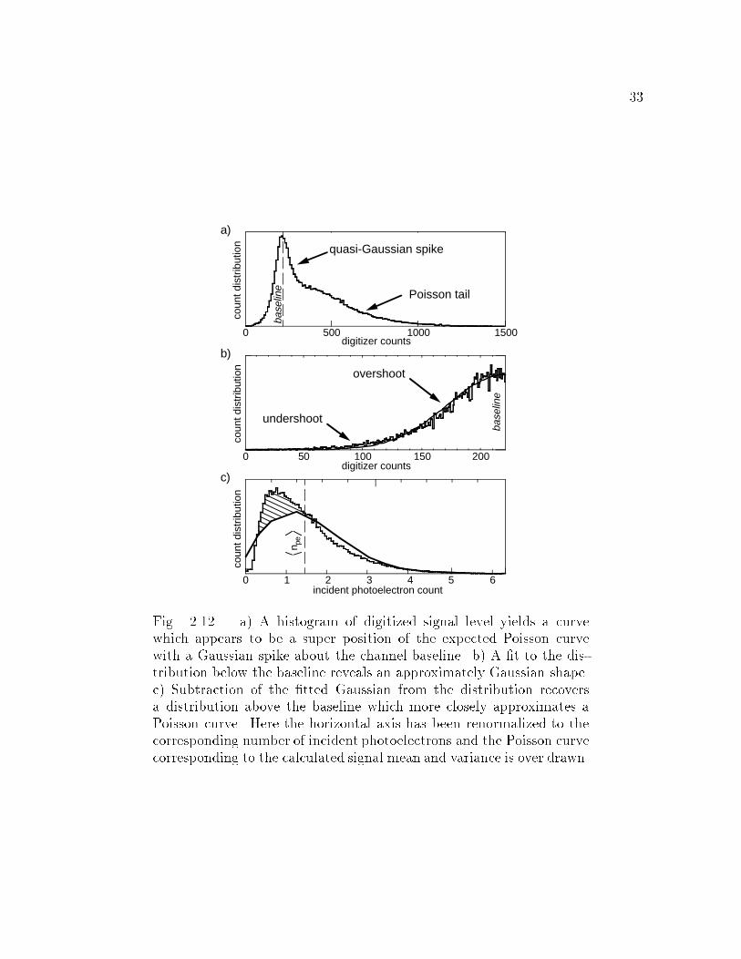
33

0 1000500 1500

500 100 150 200

digitizer counts

digitizer counts

incident photoelectron count

coun

t dis

trib

utio

n

base

line

overshoot

undershoot

coun

t dis

trib

utio

nco

unt d

istr

ibut

ion

a)

b)

c)

base

line

quasi-Gaussian spike

Poisson tailn p

e

0 51 2 3 4 6

Fig. 2.12.| a) A histogram of digitized signal level yields a curvewhich appears to be a super position of the expected Poisson curvewith a Gaussian spike about the channel baseline. b) A t to the dis-tribution below the baseline reveals an approximately Gaussian shape.c) Subtraction of the tted Gaussian from the distribution recoversa distribution above the baseline which more closely approximates aPoisson curve. Here the horizontal axis has been renormalized to thecorresponding number of incident photoelectrons and the Poisson curvecorresponding to the calculated signal mean and variance is over drawn.

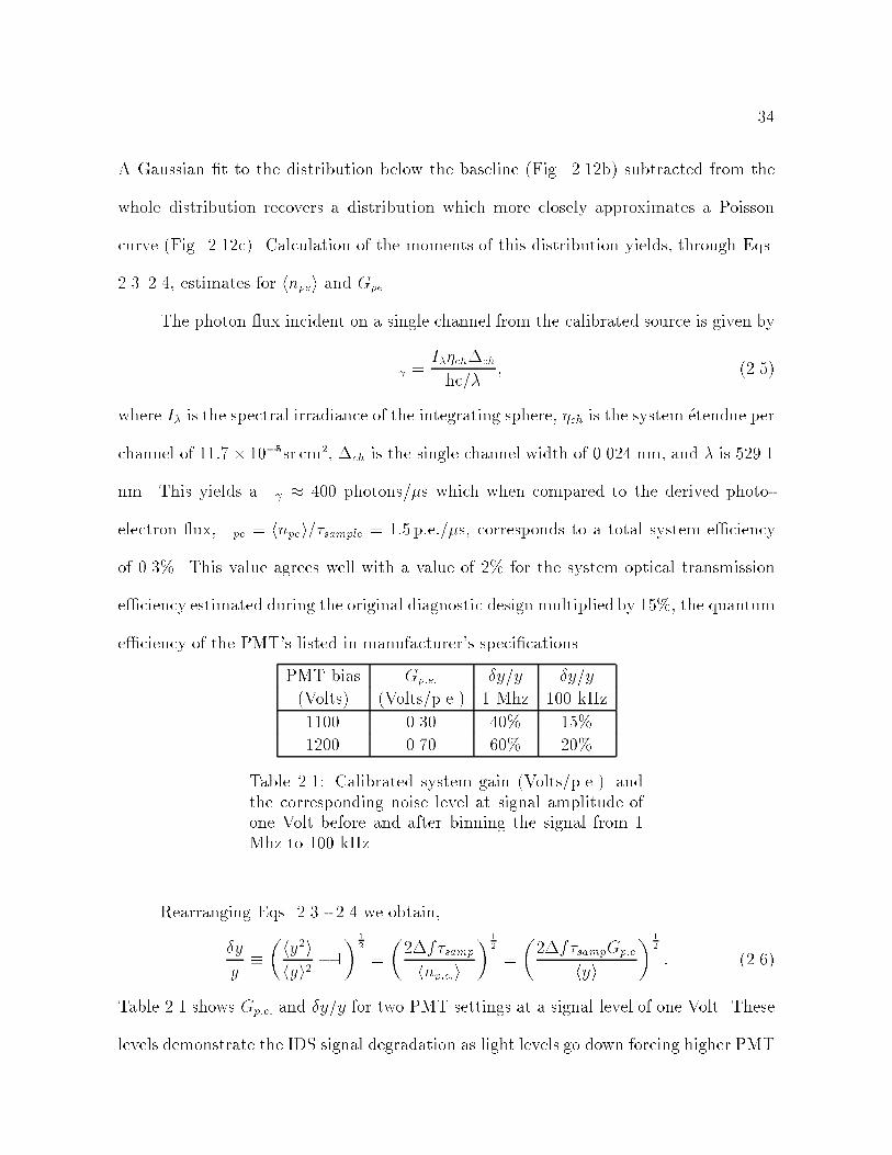
34

A Gaussian t to the distribution below the baseline (Fig. 2.12b) subtracted from the

whole distribution recovers a distribution which more closely approximates a Poisson

curve (Fig. 2.12c). Calculation of the moments of this distribution yields, through Eqs.

2.32.4, estimates for hnpei and Gpe.

The photon ux incident on a single channel from the calibrated source is given by

=Ichch

hc=; (2.5)

where I is the spectral irradiance of the integrating sphere, ch is the system etendue per

channel of 11:7 105sr cm2, ch is the single channel width of 0.024 nm, and is 529.1

nm. This yields a 400 photons=s which when compared to the derived photo-

electron ux, pe = hnpei=sample = 1:5 p:e:=s, corresponds to a total system eciency

of 0.3%. This value agrees well with a value of 2% for the system optical transmission

eciency estimated during the original diagnostic design multiplied by 15%, the quantum

eciency of the PMT's listed in manufacturer's specications.

PMT bias Gp:e: y=y y=y

(Volts) (Volts/p.e.) 1 Mhz 100 kHz

1100 0.30 40% 15%

1200 0.70 60% 20%

Table 2.1: Calibrated system gain (Volts/p.e.) andthe corresponding noise level at signal amplitude ofone Volt before and after binning the signal from 1Mhz to 100 kHz.

Rearranging Eqs. 2.3 - 2.4 we obtain,

y

yhy2ihyi2 1

1

2

=

2fsamp

hnp:e:i1

2

=

2fsampGp:e

hyi 1

2

: (2.6)

Table 2.1 shows Gp:e: and y=y for two PMT settings at a signal level of one Volt. These

levels demonstrate the IDS signal degradation as light levels go down forcing higher PMT

35

bias settings. We have generally found signal levels to be dominated by noise above a

setting of 1100 V. By binning nbin adjacent samples together one eectively increases

np:e: by nbin and decreases y=y by 1=sqrt(nbin). Of course this enhanced signal quality

comes at the cos of reduced time resolution. For uctuation measurements we typically

choose nbin = 10 retaining all uctuation power below 50 kHz. For equilibrium ow

measurements we may bin to even lower frequencies.

2.3 Data Analysis Techniques

The reduction of the raw emission proles into ion velocities and temperature occurs

in two stages. In the rst stage an automated routine ts a Gaussian prole to the

measured line shape and writes the moments of that prole to the MST database. x 2.3.1

describes the implementation of this stage. The second stage (x 2.3.4) converts these

moments into temperatures and velocities through an application of the Doppler formula.

x 2.3.2 and x 2.3.3 describe two intermediate calculations: the calibration of the unshifted

line position and the compensation for broadening of the prole by the single channel

transfer function. Finally, x 2.3.5 discusses the propagation of photon noise from the raw

signal to the derived quantities.

2.3.1 Nonlinear Curve-Fit Routine

The IDS digitizes a voltage proportional to the emission intensity of the plasma

about 16 wavelengths for each view. A robust processing engine, fit.pro, has been

developed to convert this data into physically meaningful parameters characterizing the

broadened, shifted emission line (xB.1.1). A public front-end, fit.com, denes several

variables specic to the given run (i.e. emission wavelength, PMT Voltage) before ac-

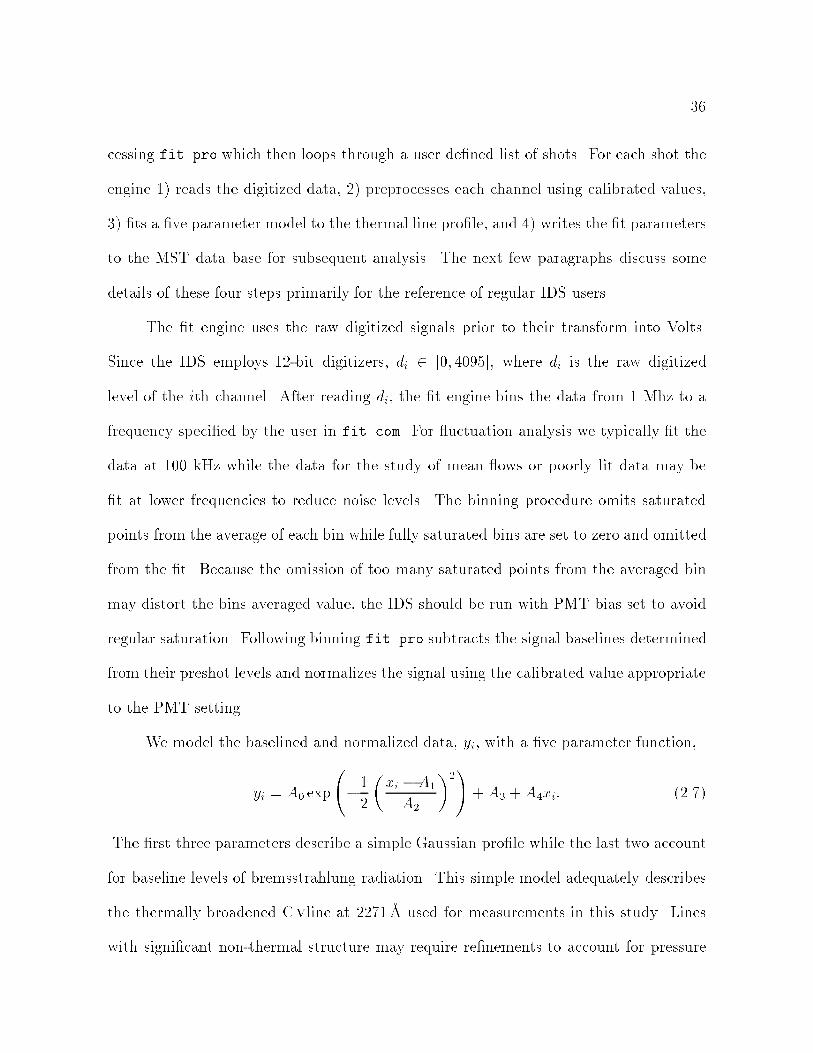
36

cessing fit.pro which then loops through a user dened list of shots. For each shot the

engine 1) reads the digitized data, 2) preprocesses each channel using calibrated values,

3) ts a ve parameter model to the thermal line prole, and 4) writes the t parameters

to the MST data base for subsequent analysis. The next few paragraphs discuss some

details of these four steps primarily for the reference of regular IDS users.

The t engine uses the raw digitized signals prior to their transform into Volts.

Since the IDS employs 12-bit digitizers, di 2 [0; 4095], where di is the raw digitized

level of the ith channel. After reading di, the t engine bins the data from 1 Mhz to a

frequency specied by the user in fit.com. For uctuation analysis we typically t the

data at 100 kHz while the data for the study of mean ows or poorly lit data may be

t at lower frequencies to reduce noise levels. The binning procedure omits saturated

points from the average of each bin while fully saturated bins are set to zero and omitted

from the t. Because the omission of too many saturated points from the averaged bin

may distort the bins averaged value, the IDS should be run with PMT bias set to avoid

regular saturation. Following binning fit.pro subtracts the signal baselines determined

from their preshot levels and normalizes the signal using the calibrated value appropriate

to the PMT setting.

We model the baselined and normalized data, yi, with a ve parameter function,

yi = A0 exp

1

2

xi A1

A2

2!+A3 +A4xi: (2.7)

The rst three parameters describe a simple Gaussian prole while the last two account

for baseline levels of bremsstrahlung radiation. This simple model adequately describes

the thermally broadened Cvline at 2271A used for measurements in this study. Lines

with signicant non-thermal structure may require renements to account for pressure

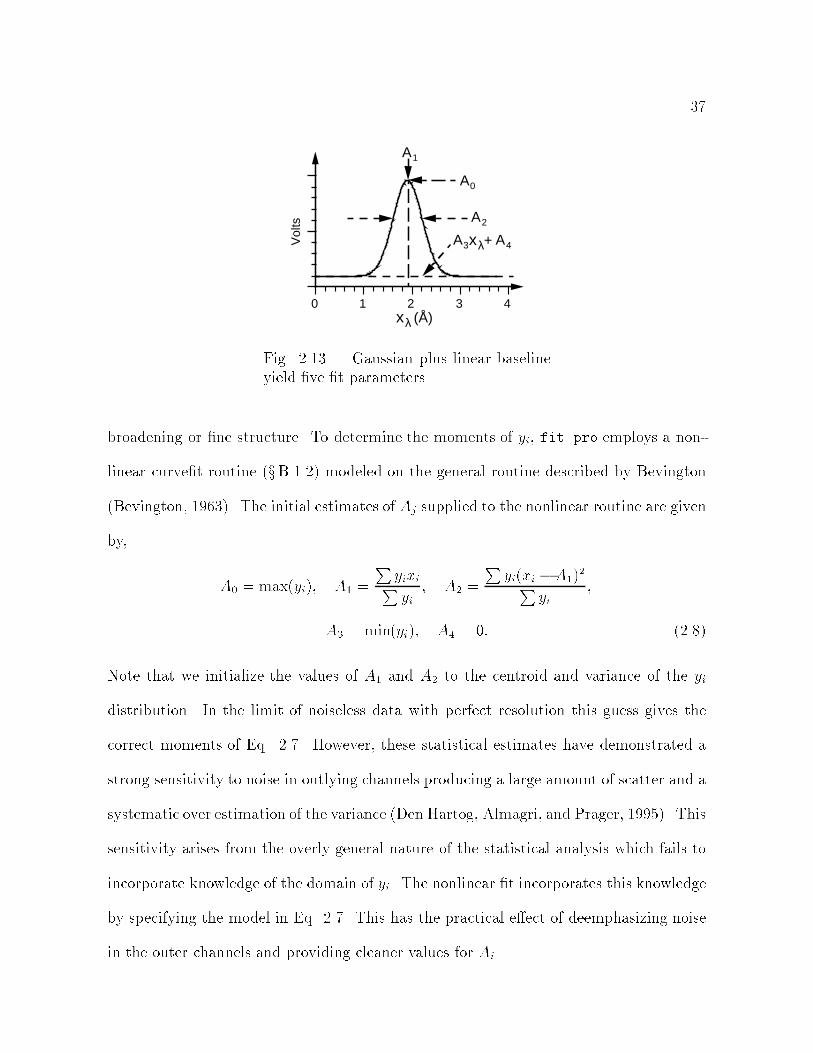
37

Vol

ts0 1 2 3 4

A0

A2

A1

xλ (Å)

A3 A4xλ+

Fig. 2.13.| Gaussian plus linear baselineyield ve t parameters

broadening or ne structure. To determine the moments of yi, fit.pro employs a non-

linear curvet routine (xB.1.2) modeled on the general routine described by Bevington

(Bevington, 1963). The initial estimates of Aj supplied to the nonlinear routine are given

by,

A0 = max(yi); A1 =

PyixiPyi

; A2 =

Pyi(xi A1)2P

yi;

A3 = min(yi); A4 = 0: (2.8)

Note that we initialize the values of A1 and A2 to the centroid and variance of the yi

distribution. In the limit of noiseless data with perfect resolution this guess gives the

correct moments of Eq. 2.7. However, these statistical estimates have demonstrated a

strong sensitivity to noise in outlying channels producing a large amount of scatter and a

systematic over estimation of the variance (Den Hartog, Almagri, and Prager, 1995). This

sensitivity arises from the overly general nature of the statistical analysis which fails to

incorporate knowledge of the domain of yi. The nonlinear t incorporates this knowledge

by specifying the model in Eq. 2.7. This has the practical eect of deemphasizing noise

in the outer channels and providing cleaner values for Ai.

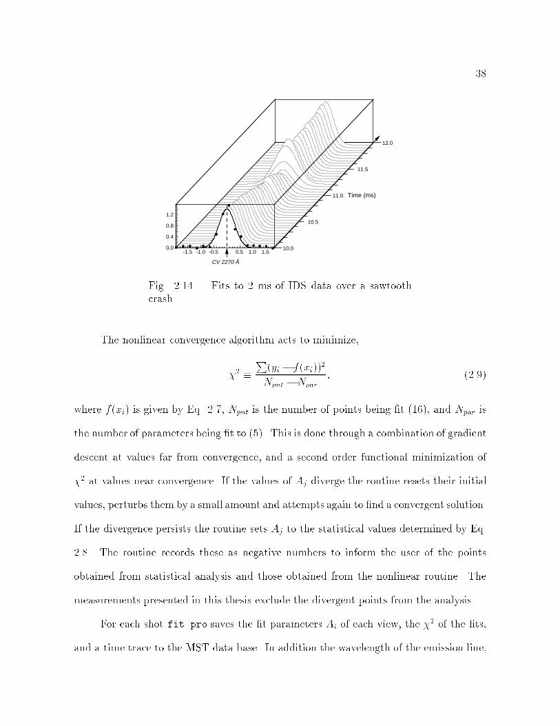
38

-1.5 -1.0 -0.5 0.5 1.0 1.5

CV 2270 Å

0.0

0.4

0.8

1.2

10.0

11.0

12.0

11.5

10.5

Time (ms)

Fig. 2.14.| Fits to 2 ms of IDS data over a sawtoothcrash.

The nonlinear convergence algorithm acts to minimize,

2 P(yi f(xi))2

Npnt Npar; (2.9)

where f(xi) is given by Eq. 2.7, Npnt is the number of points being t (16), and Npar is

the number of parameters being t to (5). This is done through a combination of gradient

descent at values far from convergence, and a second order functional minimization of

2 at values near convergence. If the values of Aj diverge the routine resets their initial

values, perturbs them by a small amount and attempts again to nd a convergent solution.

If the divergence persists the routine sets Aj to the statistical values determined by Eq.

2.8. The routine records these as negative numbers to inform the user of the points

obtained from statistical analysis and those obtained from the nonlinear routine. The

measurements presented in this thesis exclude the divergent points from the analysis.

For each shot fit.pro saves the t parameters Ai of each view, the 2 of the ts,

and a time trace to the MST data base. In addition the wavelength of the emission line,

39

the mass of the impurity ion and the calibrated position of the unshifted wavelength are

stored as scalars. Fig. 2.14 shows data t at 20 kHz spanning 2 ms. The data yi for the

rst time point shown is plotted over the tted Gaussian to illustrate typical t quality.

Note the sawtooth crash near 11 ms which broadens the distribution and increases its

amplitude. Physically this corresponds to a sharp spike in the C+4 temperature and

emissivity. Less visibly the centroids shift to the left at the crash indicating a sharp

deceleration of the plasma. The normalized 2 varies little over the sawtooth, rising only

slightly following the crash.

2.3.2 Calibration of Unshifted Emission Line Position

The Gaussian centroid, A1, is calculated in Angstroms with respect to the cali-

brated, relative positions of the 32 single channel transfer functions (Fig. 2.11). To

calculate an absolute velocity one needs to calibrate the position on that axis, x, which

corresponds to the unshifted wavelength, 0, of the observed impurity species. Knowl-

edge of x allows the user to calculate the true wavelength of the shifted centroid, 1,

as,

1 = A1 x + 0: (2.10)

The IDS facilitates the calibration of x by providing for simultaneous measurement of ion

velocity along a single toroidal chord from opposing directions. For such a measurement

one expects the red/blue shift of the line measured with one view to be equal and opposite

to the blue/red shift of the line measured with the opposing view,

Ar=b1 x = Ab=r

1 + x: (2.11)

40

This allows for the straight forward calculation of x as,

x =1

2(Ab=r

1 +Ar=b1 ): (2.12)

The engine fit.pro performs this calibration once for the shot at the beginning of the

run, reducing the noise in the calculation by averaging Eq. 2.12 over the shot,

x =1

2hAb=r

1 +Ar=b1 ishot: (2.13)

This value is written with the moments to the database for this and all subsequent shots

of the run for use in calculating the ow. The calibration may be further improved by

performing a weighted average,

x =

P(Ab=r

1 +Ar=b1 )w

2Pw

; (2.14)

where,

w =

vuut Ab=r0

b=r

!2

+

Ar=b0

r=b

!2

(2.15)

By performing the sums in Eq. 2.14 over an ensemble of several shots one may obtain a

calibration of x providing single view resolution of the ow to within a few m/s.

Several practical comments concerning the calculation of x are included here for

the benet of future IDS users. First, in performing an ensemble calculation of x or in

applying a calibration of x from one point in the run to a dierent point in the run one

must insure that the value of x is truly stationary over the shots in question. At higher

A/turn gearings of the IDS dial, a mechanical drift of the dial position has been observed

to produce a slow shot to shot drift in the position of x which can accumulate to an

equivalent ow drift of several km/s. This drift may be minimized by setting the gearing

41

of the IDS dial to a lower A/turn setting prior to the run, by positioning the IDS dial such

that its handle points down, and by avoiding bumps to the IDS spectrometer housing

during the course of the run. Even with the above precautions separate x calibrations

should be made throughout the run to check for drift. Second, for runs employing only

the opposing toroidal view setup with both views similarly illuminated calibration of x

is unnecessary. For calculation of the ion ow one must calculate,

b=r = b=r1 0 = A

b=r1 x; or

r=b = r=b1 0 = A

r=b1 x: (2.16)

However, with opposing toroidal views we may combine these expressions with Eq. 2.11

to obtain,

b=r = r=b = 1

2(Ab=r

1 Ar=b1 ): (2.17)

This expression which includes only the separation of the two centroids improves the

noise statistics of Eq. 2.16 by a factor of 1=p2 while eliminating the need for x. Eq.

2.16 should only be used when nonopposing views are employed or when light levels

(hence noise levels) of the two views dier by a large amount due to lens coatings.

Finally, uctuation studies require no calibration of x as we typically lter mean ow

contributions from the signal.

2.3.3 Deconvolution of Transfer Function from f()

The roughly triangular transfer function of each IDS channel exhibits a FWHM

approximately equal to the separation between the channels. The measured intensity

distribution is actually a convolution of the thermal distribution and this transfer func-

tion. This convolution broadens the measured distribution producing tted values of A2

42

205

50

100

200

500

1000

2000

2000

1000

500

20010050205

01

23

4Å

1.0

0.8

0.6

0.4

0.2

0.00.00.2

0.40.6

0.81.0

actual variance (Å)

measured variance (Å)

Fig.

2.15.|Finite

width

transfer

function

sact

tosligh

tlybroad

entherm

allines.

Show

n(left)

aresim

ulated

(gray)andtted

(black

)lines

ofCvat

20eV

,100

eV,

and500

eV.Mappingof

tted

values

(right)isaccom

plish

edwith

poly

nom

ialtto

simulated

values.

Broad

eningbecom

esinsign

ican

tat

high

temperatu

res.

which

aresystem

aticallylarger

than

thetru

edistrib

ution

variance .

Fig.

2.15ashow

s

thetran

sferfunction

sfor

therst

16IDSchannels

plotted

versuswavelen

gth.Three

sets

ofdistrib

ution

sare

plotted

overthetran

sferfunction

scorresp

ondingto

Cvtem

peratu

res

of20

eV,100

eV,and500

eV.Thegrey

curve

ineach

setcorresp

ondsto

theorigin

al

simulated

distrib

ution

s.These

distrib

ution

swere

then

convolved

numerically

with

the

transfer

function

toobtain

asim

ulated

sixteen

poin

tmeasu

rement.

Thismeasu

rement

was

then

tas

describ

edabove

toobtain

atheGaussian

distrib

ution

plotted

inblack

.

For

eachcase

thetted

distrib

ution

isbroad

erthan

theorigin

although

thedieren

ce

atthetwohigh

ertem

peratu

resisbarely

visib

le.Tocorrect

forthisbroad

eningweneed

amappingfrom

themeasu

redvarian

ceto

theactu

alvarian

ceof

thedistrib

ution

.Fig.

2.15bshow

sthree

mappings

forA2valu

escorresp

ondingto

Cvtem

peratu

resfrom

5eV

to2keV

where

thedash

edlinecorresp

ondsto

theidentity

map,

=A2 :

(2.18)

43

By approximating the transfer functions with Gaussians we may analytically calculate

this mapping to be, since the convolution of two Gaussians is a Gaussian,

=qA22 2t:f:; (2.19)

where t:f: is the typical variance of a Gaussian t to the measured transfer functions.

This mapping is shown with the grey line in Fig. 2.15b for a t:f: 0:2. Note, this

curve would map an apparent temperature of 100 eV down to an actual temperature

of 10 eV though the eect becomes less dramatic at higher temperatures. To test Eq.

2.19 we performed simulated measurement over the range of variances shown to obtain

an empirical mapping. Surprisingly, this mapping, shown in black, is much closer to the

identity map of Eq. 2.18 than the quadratic map of Eq. 2.19. This result currently

lacks a satisfactory explanation although suspicion centers on the discrete sampling of

the convolved Gaussian by the 16 channels. By tting a third order polynomial to the

simulated points we are able to apply this mapping to A2 before converting those values

to temperatures

2.3.4 Doppler Formula

After calculating and from A1 and A2 as described above, we may describe

the distribution of radiated light as,

f() / exp

( 0 )2

22

!: (2.20)

To convert Eq. 2.20 into a velocity distribution we employ the Doppler formula,

v =

00

c; (2.21)

44

to rewrite Eq. 2.20 as,

f(v) / exp

0B@

v c

0

22c 0

21CA : (2.22)

We may use this distribution to solve for the expectation value of v,

hvi =Rdv v f(v)Rdv f(v)

=c

0; (2.23)

and the expectation value of v2,

hv2i =Rdv v2 f(v)Rdv f(v)

=

c 0

2

: (2.24)

Thus, and yield our impurity velocity and temperature respectively as,

vZ =c

0 3:0 105

0

km=s; (2.25)

TZ = mZ

c 0

2

9:3 108mZ

0

2

eV; (2.26)

where all wavelengths are in Angstroms andmion is in amu. These calculations performed

in the post-processing routine [jchapman.public.flow]flow.pro (xB.1.3).

2.3.5 Error Propagation

Optical noise in the raw IDS signal propagates through the nonlinear t routine to

produce substantial noise levels in the the centroid and variance returned by the routine.

We have relied on montecarlo simulation techniques to observe the behavior of the error

propagation. For these simulations we generated thermal distributions corresponding

to Cvdistributions with temperatures from 50 eV to 500 eV and random velocities of

several km/s. To these distributions we added white Poisson noise of various levels to

simulate the optical noise in the input channels. We discovered that dened as,

p2

A0; (2.27)

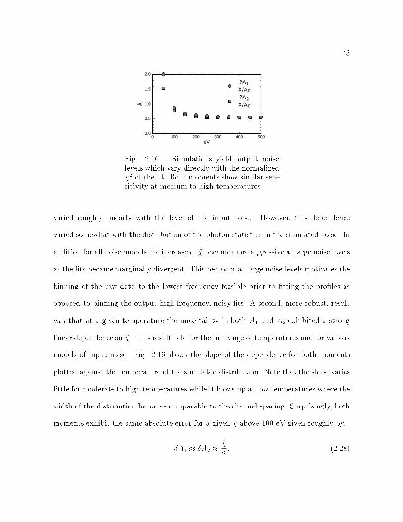
45

0 100 200 300 400 500

δA1χ /A0

δA2χ /A0

0.0

0.5

1.0

1.5

2.0

ÅeV

Fig. 2.16.| Simulations yield output noiselevels which vary directly with the normalized2 of the t. Both moments show similar sen-sitivity at medium to high temperatures.

varied roughly linearly with the level of the input noise. However, this dependence

varied somewhat with the distribution of the photon statistics in the simulated noise. In

addition for all noise models the increase of became more aggressive at large noise levels

as the ts became marginally divergent. This behavior at large noise levels motivates the

binning of the raw data to the lowest frequency feasible prior to tting the proles as

opposed to binning the output high frequency, noisy ts. A second, more robust, result

was that at a given temperature the uncertainty in both A1 and A2 exhibited a strong

linear dependence on . This result held for the full range of temperatures and for various

models of input noise. Fig. 2.16 shows the slope of the dependence for both moments

plotted against the temperature of the simulated distribution. Note that the slope varies

little for moderate to high temperatures while it blows up at low temperatures where the

width of the distribution becomes comparable to the channel spacing. Surprisingly, both

moments exhibit the same absolute error for a given above 100 eV given roughly by,

A1 A2

2: (2.28)

46

When one then propagates A1 and A2 through Eqs. 2.25Eq. 2.26, one obtains a

relative sensitivity of ion velocity to input noise which is far stronger than the sensitivity

of temperature as . In practice these simulation results have led us to measure

the noise oor of the ion velocity power spectrum to characterize the overall noise power,

and then to distribute that power in time proportional to (t) (Eq. 2.27).

2.4 Minority Species Dynamics

Diculties stemming from Hydrogen's 13.6 eV ionization potential impede direct

spectroscopic measurements of the majority species. Almost all of the Hydrogen ionizes

in the cool plasma edge producing an intensity distribution dominated by a large cold

spike. Charge exchange of core ions does produce a hot secondary distribution re ecting

dynamics in the MST interior. However, this eect may only be resolved in the wings of

the total distribution after several e-foldings of the cold primary distribution. Attempts

to characterize the temperature of this secondary distribution have been inconclusive as

the low radiation levels in the wings of the hot distribution barely register with the IDS.

An eort to discern ion ow from this distribution would prove daunting, and resolving

fast uctuations in that ow more daunting still. Consequently, the IDS design optimally

resolves UV radiation emitted from ionized minority species intrinsic to the MST plasma.

These species possess a wide range of ionization potentials allowing measurement of

dierent regions in the plasma through the selection of dierent spectral lines.

2.4.1 Perpendicular Flow for Dierent Species

Our desire to characterize the ow behavior of the majority species motivates us to

relate this behavior to that of the observed minority species. A simple general argument

47

may be advanced from the equation governing the perpendicular ow in each species,

vZ;? =EB

B2+

Br p0ZeB2ZnZ

; (2.29)

where the prime denotes a radial derivative. Simple estimates of Eq. 2.29 indicates the

ow over the interior of the plasma to be driven predominantly by the species independent

EB term. In addition we anticipate the velocity uctuations contributing to the

dynamo to be ~EB (x 1.2.2) driven, suggesting that the uctuation results presented

here may be generalized to the majority species. Near the edge, pressure gradients

become signicant yielding a nontrivial diamagnetic contribution. The diamagnetic term

may be expanded as,

vZ;rp =Br TZeB2Z

n0ZnZ

+T 0Z

TZ

; (2.30)

yielding a dependence on the normalized temperature and density gradients with an

overall multiplier of TZ=Z. In general Ti evolves gradually and we can expect through

thermal equilibration that TZ Ti2, reducing the dependence of the second term to T 0

i=Z.

This eect should predominate near the edge where Ti drops dramatically potentially

yielding an under-representation of the bulk ow (Z =+ 1) by the minority species

(Z + 2). The second term depends on the normalized derivative of the emission prole

which varies widely amongst species. Species like C+4 which radiate near the core tend to

have broad emission proles with correspondingly small values of n0Z=nZ . On the other

hand, species like Ciii radiate from narrow shells near the edge with two large gradients

in nZ delineating their radial boundaries. These gradients produce opposing vZ;rp's of

2While thermalization does not hold TZ Ti during a sawtooth crash when ion heating proceedsmore rapidly than energy thermalization, CXA measurements of Ti during the crash indicate that themajority species exhibits sawtooth dynamics similar to those observed in the minority.

48

ni Ti =iS (kHz)

(1019m3) (eV) C+4 C+2 B+3 O+4

0.2 20 33.5 8.4 20.9 25.1

0.5 120 5.7 1.4 3.6 4.3

0.8 200 4.2 1.1 2.6 3.2

1.1 350 2.5 0.6 1.6 1.9

Table 2.2: =iE for edge plasma and three core plasma conditions

with mi = Zi = 1 and lni = 16.

roughly equal magnitudes separated by only a few cm's . As the IDS line of sight will

pass through both ows this contribution should nearly cancel producing only a slight

broadening in the measured line prole.

2.4.2 Energy and Momentum Relaxation

Eq. 2.29 omits cross-species collisional terms which could produce parallel ows

in MST similar in magnitude to v?. These collisional terms also act to equilibrate the

temperature between species. Here we will determine the typical relaxation rates for the

energy and momentum of two dierent thermal species. The energy relaxation rate for

two thermal distributions is given by the expression (Callen, 1997),

=E =

n q2q

2 ln

3

2 2omm v3T

; (2.31)

where,

vT (v2T + v2T)1

2 =

2Tm

+2Tm

1

2

: (2.32)

From Eq. 2.32 we can see that the minority species will equilibrate far more rapidly to

the ion uid than the electron uid with,

=iE mi

me

3

2

=eE : (2.33)

49

Z (A) Z mZ (amu) UZ (eV)

C iii 2296.9 +2 12.011 47.9

Ov 2781.0 +4 15.999 113.9

B iv 2821.7 +3 10.811 259.3

Cv 2270.9 +4 12.011 392.0

Table 2.3: The wavelength, charge, mass, and ionization poten-tial for the four commonly observed impurity emission lines.

For the case of an impurity species equilibrating with the majority ions Eq. 2.31 becomes,

=iE =

ni e4 Z2

Z2i lni

3

2 2ommi v3Ti 2 106

nim

1

2

i Z2Z

2i lni

mT3

2

i

!s1; (2.34)

where,in the nal expression, masses are given in amu, temperatures in eV, and densities

in 1019m3. Eq. 2.34 assumes T Ti and m mi allowing the approximation of

Eq. 2.32 by vTi (2Ti=mi)1=2. The momentum relaxation rate of two thermal species

is given by

=S =n q

2q

2 ln

33

2 2omm v3T

; (2.35)

where,

m mm

m +m: (2.36)

Thus the momentum relaxation rate of the minority species with the bulk ions is given

by,

=iS =

ni e4 Z2

Z2i lni

33

2 2ommi v3Ti

=iE

3 7 105

nim

1

2

i Z2Z

2i lni

mT3

2

i

!s1: (2.37)

where we again assume m mi for which Eq. 2.36 simplies to mi mi. Note that

the ion velocity equilibrates roughly three times more slowly than the ion energy.

Table 2.2 shows approximate momentum relaxation rates for four commonly ob-

served impurity species in dierent plasma conditions. The top row is representative of

50

cool edge conditions while the remaining three rows match the hotter conditions in the

core for increasing plasma current. The bulk plasma ow typically equilibrates with im-

purities in < 1ms, fast enough to insure that the mean parallel ows and temperatures

of dierent species match over the shot. However, collisional equilibration alone does

not insure that rapid ( 10s) dynamics at the sawtooth crash proceed identically in all

species.

2.4.3 Impurity Emission Proles

Limited control over the spatial resolution of the IDS is achieved through the se-

lection of the impurity species viewed. While impurities like C+4 with high ionization

potentials should be found predominantly in the MST core, easily ionized species like

Ciii should be constrained to a relatively thin shell near the plasma edge. The Impurity

Monochromator Array (IMA) was developed to measure these distributions by collecting

light along ve poloidal chords (Woehrer, 1996). The impact parameters of the chords

extends from ri=a = 0:00 to ri=a = 0:82 providing reasonable coverage of the core region

and comparatively poor resolution of the edge. Light collected along the ve chords is

transmitted through ber optics to the monochromators where radiation of the desired

wavelength is converted by PMT's into the measured signal. A coarse relative calibration

of the ve PMT's is improved by rotating the chords viewed by each PMT every few shots

and analyzing the data in an ensemble which spans several rotations.3 Light levels from

the ve channels are then inverted into an eleven point prole using a procedure which

combines a spline t with Abel inversion.

3I have developed an improved in situ calibration procedure which may be conducted at the be-ginning of the run to avoid rotation. The code associated with this procedure may be found in[jchapman.public.imp mono]cal mono.pro.

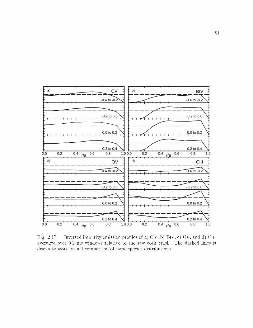
51

CV

OV

a)

c) d)

b)

CIII

BIV

-0.4 to -0.2

-0.2 to 0.0

0.0 to 0.2

0.2 to 0.4

-0.4 to -0.2

-0.2 to 0.0

0.0 to 0.2

0.2 to 0.4

-0.4 to -0.2

-0.2 to 0.0

0.0 to 0.2

0.2 to 0.4

-0.4 to -0.2

-0.2 to 0.0

0.0 to 0.2

0.2 to 0.4

0.0 0.2 0.4 0.6 0.8 1.0r/a 0.0 0.2 0.4 0.6 0.8 1.0r/a

0.0 0.2 0.4 0.6 0.8 1.0r/a 0.0 0.2 0.4 0.6 0.8 1.0r/a

Fig. 2.17.| Inverted impurity emission proles of a) Cv, b) Biv, c) Ov, and d) Ciiiaveraged over 0.2 ms windows relative to the sawtooth crash. The dashed lines isdrawn to assist visual comparison of same species distributions.

52

Fig. 2.17 shows the ve chord inverted proles for the four impurities commonly

measured by the IDS (Table 2.3). The proles were averaged over four 200 s long win-

dows centered about the sawtooth. Cv is the most broadly distributed with signicant

emission from the core, though the peak emission occurs at r=a 0:6. BIV also emits

from a broad region though its prole is more hollow. While proles of both OV and

CIII are edge peaked and therefore poorly resolved, the ratio of light from the outer to

inner chord is higher for CIII indicating that it is more edge peaked. The rise in the CIII

prole near the core is probably an artifact of the inversion process coupled with errors in

the normalization. While radiation levels rise overall at the sawtooth crash their radial

distributions exhibit little change allowing the conclusion that the radial location of the

IDS measurements remains stationary over the sawtooth cycle.

2.4.4 Flow and Temperature Proles

-10

0

10

20

ion

velo

city

(km

/s)

CV

BIV

OV

CIII

-2 -1 0 1 2time (ms)

300

200

100

0-2 -1 0 1 2

time (ms)

ion

tem

pera

ture

(eV

)

CV

BIV

OVCIII

Fig. 2.18.| Impurity a) ow and b) temperature over a sawtooth crash showscore species owing more rapidly at higher temperatures than those near the edge.

Fig. 2.18 shows the measured toroidal ows and temperatures of the four impurity

species ensembled over a sawtooth crash. The ow speed of the impurities decreases

as one moves from the core to the edge of the plasma with CIII actually owing in a

direction opposite to that of the core ions. The direction of the core ions corresponds to

53

an ErB drift as indicated in Eq. 2.29. At the sawtooth crash the ion ow decelerates

5 km/s for each of the species. This does not appear to represent a locking to the lab

frame as evidenced by Ciii which actually accelerates relative to the shell at the crash.

The deceleration appears abruptly in the edge species and then appears to propagate

inward toward the core. The deceleration may produced by the viscous coupling of the

ion uid with the core tearing modes. The temperature proles all exhibit the anomalous

heating spike at the sawtooth crash. Note the temperatures of the ions are colder towards

the edge with the Ciii temperature of order 10 eV. Finally, note the temperature of the

impurities peaks later as we move toward the core of the plasma.

2.5 Passive Chord Averaging

While passive collection of radiation enables nonperturbing measurements of core

dynamics, the chord averaged nature of the measurement compromises the spatial reso-

lution of the IDS. The IDS line of sight averages over small scale uctuation structures

and attenuates low k structures by a factor that depends on both the wavenumber of

the mode and its radial structure. In addition the simultaneous sampling of dierent

phases of the velocity uctuation raises the question of how the ultimate phase of the

chord averaged measurement relates to the phase at a known reference point. Finally,

we expect toroidal, poloidal, and radial chords to measure ~v, ~v, and ~vr, respectively.

However, casual inspection reveals nonzero projections of r and onto the toroidal chord

and r onto the poloidal chord. How does the chord blend these dierent components

together? This section develops exact expressions relating the chord averaged IDS mea-

surements to to the local velocity uctuation structures. These expressions embody two

key results. First, a line integral of ~v over the line of sight may be replaced by a radial

54

convolution with a known instrument function, wn. Second, the phase of the chord av-

eraged measurement matches the local uctuation phase at a point of symmetry dened

below. Later in this thesis these results will enable an estimation of the relative phase

and amplitude of h~v~bi in the core.

In the following sections we rst demonstrate analytically that by tting a Gaus-

sian prole to a chord averaged emission prole, we eectively recover the line averaged

velocity and temperature of the observed impurity. Next, we employ this result in out-

lining the general procedure for calculating the instrument function of a line of sight. We

then derive and present wn for the toroidal chord, followed by an analogous, though far

simpler, presentation for the poloidal and radial chords.

2.5.1 Integrated Emission Proles

The distribution in wavelength of line radiation from the observed impurities should

be a Doppler broadened and shifted Gaussian, provided thermal broadening dominates

other sources of line structure. We represent this distribution at some point l with the

expression,

f(; l) = Af(l) exp

( f (l))2

22f (l)

!: (2.38)

The IDS integrates f(; l) along its line of sight obtaining,

hf()i =Zdlf(; l); (2.39)

which is not generally Gaussian. For example, the \two temperature" distribution of the

H line exhibits a large narrow distribution corresponding to ionization at the cool edge.

However, away from the spike, the wings of the distribution correspond to hot, charge-

exchange ions in the core. Despite this fact, we routinely observe integrated distributions

55

of core and edge impurities to be extremely well t by a Gaussian function, providing

ion velocities and temperatures which we believe to re ect local ion dynamics. In the

following paragraphs we derive expressions relating the moments of the Gaussian t of

hf()i to the local moments of the impurity emission. These expressions conrm that, to

good approximation, the moments of the t correspond to the line integrated moments

of the local distribution.

Here we derive these moments providing intuitive results, modied only slightly

by the more rigorous treatment which follows. First we dene the intensity of impurity

emission at a point along the line of sight by the integral of f() over ,

If(l) =

Zdf(; l) =

p2f (l)Af(l); (2.40)

where f() is a Gaussian with local amplitude, Af(l), and variance, f(l). Now we

retrieve the centroid of the the line-integrated distribution by calculating its rst moment

with ,

hf i =Rd

Rdlf(; l)R

dRdlf(; l)

=

RdlIf(l)f(l)RdlIf(l)

; (2.41)

where f (l) is the local centroid of f(). This matches our expectation that the centroid

of hf()i equals the path averaged centroid of f() weighted by If(l). Calculating the

second moment of hf()i we nd,

hf i =Rd( hf il)2

Rdlf(; l)R

dRdlf(; l)

=

RdlIf(l)

2f(l) + (f (l) hf il)2

RdlIf(l)

: (2.42)

The rst term on the RHS gives the chord averaged variance of f() weighted by If()

in direct analogy to Eq. 2.41. The second term re ects the broadening of the integrated

distribution by variations in the velocity prole over the line of sight. A instance of such

broadening was mentioned for the case of CIII which exhibits opposite diamagnetic ows

56

of similar magnitude at the boundaries of its emission shell. In a limiting case of two CIII

shells of equal brightness moving with respect to each other at 10 km/s, the broadening

due to this term yields a temperature enhancement of 1.5 eV. Thus, except for cases

of cold ions with extremely sheared velocity proles, this term should be dominated by

the line averaged variance.

As discussed in x2.3 the distribution moments calculated directly from hfil prove

overly sensitive to noise in the distribution. Therefore, we t the distribution to a Gaus-

sian, g(), and employ the moments of that Gaussian in our subsequent calculations.

Here we derive rigorous expressions for these moments by performing analytically what

fit.pro performs numerically. This entails minimizing,

2 =

Zd (g hfil)2; (2.43)

with respect to the amplitude (Ag), centroid (g), and variance (g) of g(). Setting the

partial derivatives of 2 with respect to the three parameters equal to zero, yields the

minimization condition,

Zdmg hfil =

Zdmg2; m 2 f0; 1; 2g: (2.44)

We may perform the RHS integrals easily to obtain the moments of g2. To evaluate the

LHS integrals we place the product g hfil into the form of a Gaussian,

g hfil =Zdl Afg exp

( fg)2

22fg

!; (2.45)

57

where,

Afg = AgAf exp

(f g)2

2(2f + 2g)

!; (2.46)

fg =2gf + 2fg

2f + 2g(2.47)

fg =fg

(2f + 2g)1=2: (2.48)

The near unity exponential term in Eq. 2.46 results from completing the square to obtain

the Gaussian exponent of Eq. 2.45. Using Eq. 2.45 - 2.48 we may evaluate the LHS of

Eq. 2.44 to obtain three simultaneous equations:

p2

ZdlAfgfg = A2

gg; (2.49)

p2

ZdlAfgfgfg = A2

ggg; (2.50)

p2

ZdlAfgfg(

2fg + 2fg) = A2

gg(2g + 2g=2): (2.51)

These equations may be combined and rearranged to obtain implicit expressions for g

and g:

g =

Rdl I 0f fRdl I 0f

; (2.52)

2g =

Rdl I 0f

2f + 2(2f 2g) 2(fg)

2

1+2g=2

f

Rdl I 0f

: (2.53)

The weighting function, I 0f , is given by,

I 0f =p2Af f exp

(f g)2

2(2f + 2g)

! 1

2+

2f22g

3

2

: (2.54)

This diers from If (Eq. 2.40) by two factors which deviate weakly from unity where

f(; l) deviates from g(). Except for these small corrections to I 0f , Eq. 2.52 replicates

Eq. 2.41. Likewise, Eq. 2.53 mirrors Eq. 2.42 except for the the weak dependence

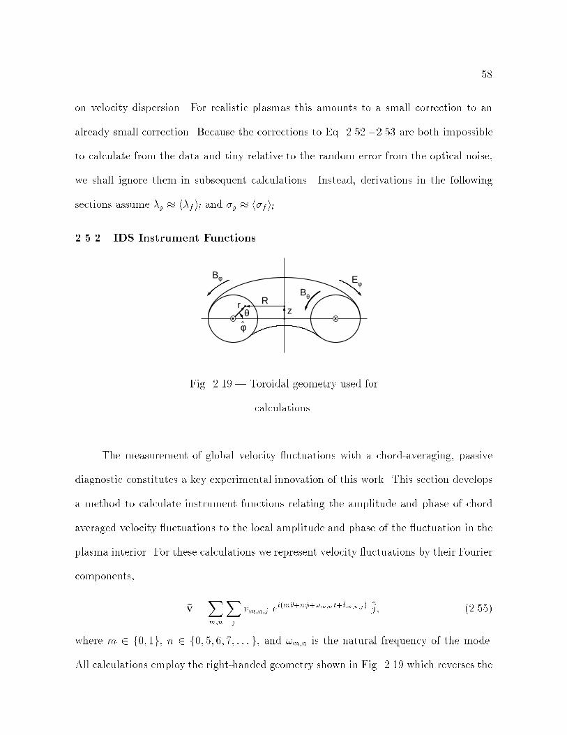
58

on velocity dispersion. For realistic plasmas this amounts to a small correction to an

already small correction. Because the corrections to Eq. 2.52 - 2.53 are both impossible

to calculate from the data and tiny relative to the random error from the optical noise,

we shall ignore them in subsequent calculations. Instead, derivations in the following

sections assume g hf il and g hf il.

2.5.2 IDS Instrument Functions

zRr

Bθ

Bφ Eφ

φθ

Fig. 2.19.| Toroidal geometry used for

calculations.

The measurement of global velocity uctuations with a chord-averaging, passive

diagnostic constitutes a key experimental innovation of this work. This section develops

a method to calculate instrument functions relating the amplitude and phase of chord

averaged velocity uctuations to the local amplitude and phase of the uctuation in the

plasma interior. For these calculations we represent velocity uctuations by their Fourier

components,

~v =Xm;n

Xj

vm;n;j ei(m+n+!m;n t+m;n;j ) j; (2.55)

where m 2 f0; 1g, n 2 f0; 5; 6; 7; : : : g, and !m;n is the natural frequency of the mode.

All calculations employ the right-handed geometry shown in Fig. 2.19 which reverses the

59

sense of the poloidal angle from that of the MST naming convention. For these, both

vm;n;j and m;n;j are considered arbitrary functions of radius which are constant on a ux

surface.

We now consider the chord averaged value of a single Fourier component from the

sum in Eq. 2.55. For a particular chord the chord average may be written,4

~vx =1

2Lx

Z +Lx

Lx

dlx IZXj

~vj lx j; (2.56)

where, for convenience, we omit the normalization integral of the impurity emission, IZ

and drop the m and n subscripts. In these expressions x 2 fT; P;Rg, where T , P , and

R are labels for the toroidal, poloidal, and radial chords respectively. We may expand

the jth component of the sum in Eq. 2.56 yielding,

~vx;j =1

2Lx

Z +Lx

Lx

dlx IZ vjeij ei(m(x)+n(x)) lx j

ei(mx+nx+!t); (2.57)

where we have extracted the xed angles x and x from the integral. We dene these

angles to satisfy the symmetry conditions,

x = ((lx) + (lx))=2; (2.58)

x = ((lx) + (lx))=2: (2.59)

Physically, this symmetry anchors the phase of the chord averaged signal to the local

uctuation phase at = x, = x by insuring the exact cancellation of phase contri-

butions from lx by those at lx. Mathematically, the symmetry permits Eq. 2.57 to be

4This expression employs Eq. 2.41 to equate the measured centroid of the integrated intensity distri-bution to the the line averaged centroid of the local distribution weighted by the local emission intensity.

60

rewritten as,

~vx;j =1

a

Z a

ro;x

dr IZ vjeij wj;x e

i(mx+nx+!t); (2.60)

where ro;x is the impact radius of the chord. The instrument function, wj;x, incorporates

three eects: the projection of j onto the line of sight, the radial weighting of the line of

sight (dlx=dr), and the intersection of the m, n mode with the line of sight. Each eect

depends solely on the known geometry of the chord, making it possible to calculate wj;x

exactly. By casting the line integral into the form of Eq. 2.60 we have converted the

complex and somewhat arduous task of accounting for a line integral into the one-time

task of calculating wj;x for each chord. Substituting Eq. 2.60 back into Eq. 2.56 we

obtain the complete expression,

~vx =Xm;n

1

a

Z a

ro;x

dr IZXj

vm;n;je

im;n;j wm;n;j;xei(mx+nx)

ei!t: (2.61)

This expression contains the properly weighted contribution of each component and each

Fourier mode to the measured signal.

We may also be interested in the sensitivity of the chord to modes parallel and

perpendicular to the mean magnetic eld. Given a model of B, the appropriate instru-

ment function may be determined readily from the geometric functions derived above.

Using a cylindrical model of the mean eld where, B = B(r)+B(r), the parallel (k),

cross-eld (^), and perpendicular (?) instrument functions are given by:

wk;x = b w = (Bw;x +Bw;x)=B; (2.62)

w^;x = (r b) w = (Bw;x Bw;x)=B; (2.63)

w?;x = r w = wr;x: (2.64)

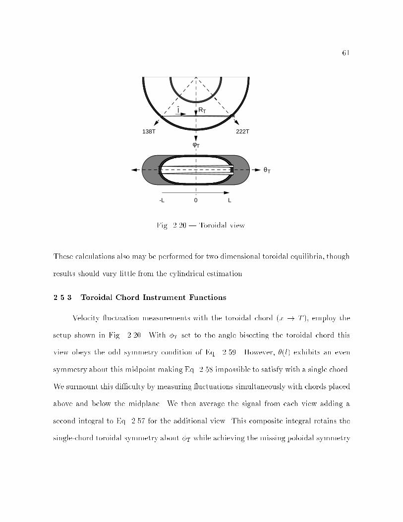
61

φT

θT

l

0-L L

138T 222T

RT

Fig. 2.20.| Toroidal view.

These calculations also may be performed for two dimensional toroidal equilibria, though

results should vary little from the cylindrical estimation.

2.5.3 Toroidal Chord Instrument Functions

Velocity uctuation measurements with the toroidal chord (x ! T ), employ the

setup shown in Fig. 2.20. With T set to the angle bisecting the toroidal chord this

view obeys the odd symmetry condition of Eq. 2.59. However, (l) exhibits an even

symmetry about this midpoint making Eq. 2.58 impossible to satisfy with a single chord.

We surmount this diculty by measuring uctuations simultaneously with chords placed

above and below the midplane. We then average the signal from each view adding a

second integral to Eq. 2.57 for the additional view. This composite integral retains the

single-chord toroidal symmetry about T while achieving the missing poloidal symmetry

62

with,

T = (top(lT ) + bot(lT ))=2 = : (2.65)

Physically toroidal phase contributions from one half of each chord exactly cancel contri-

butions from the other half, while poloidal phase contributions from the top chord cancel

contributions from the bottom chord.

The projections of , , and r onto lT are given by,

lT = +cos( T ); (2.66)

lT = sin( T ) sin( T ); (2.67)

lT r = +sin( T ) cos( T ); (2.68)

where we have chosen to align lT and at T . Inserting Eq. 2.66 with Eq. 2.57, modied

to include both chords, we employ the symmetry about T and T to collapse

the composite integral over two chords into a single integral over half of one chord,

~vT; =1

LT

Z LT

0

dlT IZ vei cos(m( T )) cos(n( T )) cos( T )

ei(mT+nT+!t): (2.69)

Likewise, inserting Eqs. 2.67-2.68 we obtain analogous expressions for ~vT; and ~vT;r.

Changing the variable of integration from lT to r these expressions may be cast into the

form of Eq. 2.60,

~vT;j =1

a

Z a

ro;T

dr IZ veij wT;j ei(mT+nT+!t); (2.70)

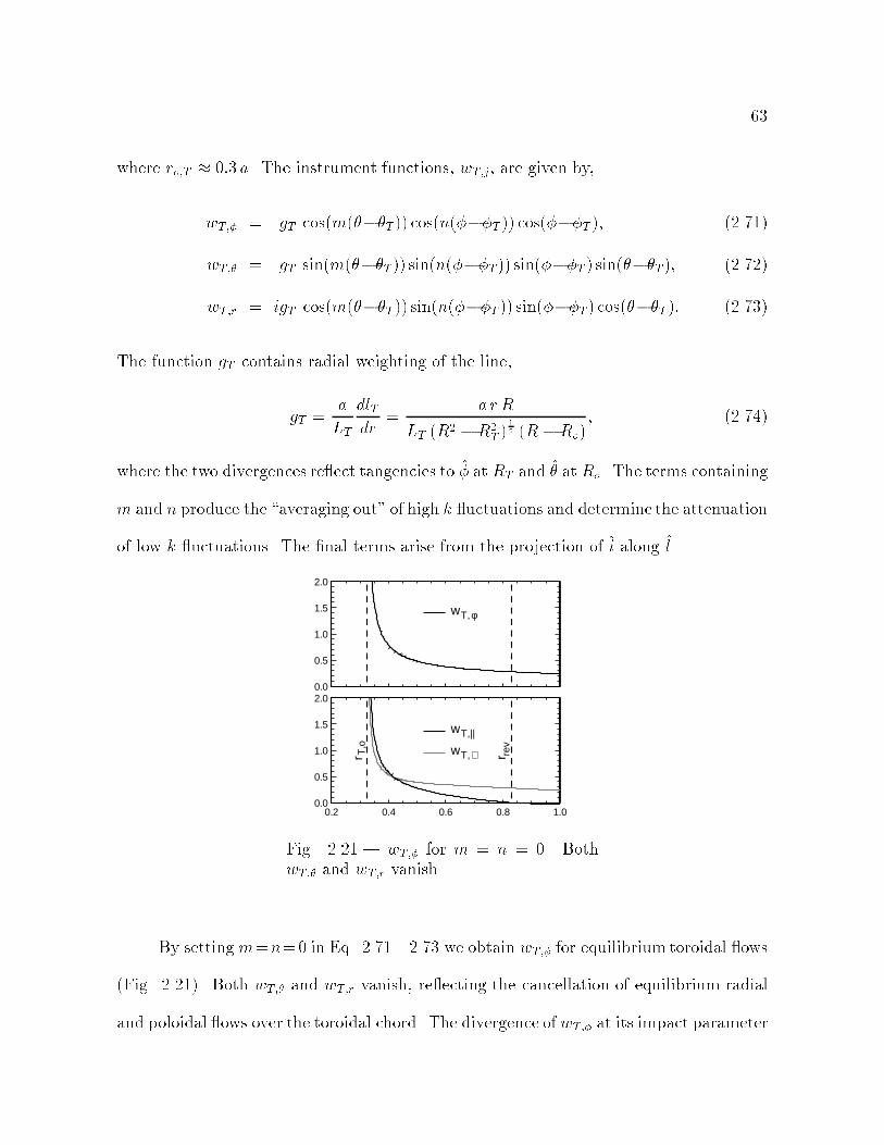
63

where ro;T 0:3 a. The instrument functions, wT;j, are given by,

wT; = gT cos(m(T)) cos(n(T )) cos(T ); (2.71)

wT; = gT sin(m(T)) sin(n(T )) sin(T ) sin(T); (2.72)

wT;r = igT cos(m(T)) sin(n(T )) sin(T) cos(T ): (2.73)

The function gT contains radial weighting of the line,

gT =a

LT

dlTdr

=a rR

LT (R2 R2T )

1

2 (R Ro); (2.74)

where the two divergences re ect tangencies to at RT and at Ro. The terms containing

m and n produce the \averaging out" of high k uctuations and determine the attenuation

of low k uctuations. The nal terms arise from the projection of i along l.

2.0

1.5

1.0

0.5

0.0

0.2 0.4 0.6 0.8 1.0

2.0

1.5

1.0

0.5

0.0

wT,φ

wT,||

wT, ∧r T,o

r rev

Fig. 2.21.| wT; for m = n = 0. BothwT; and wT;r vanish.

By setting m=n=0 in Eq. 2.71 2.73 we obtain wT; for equilibrium toroidal ows

(Fig. 2.21). Both wT; and wT;r vanish, re ecting the cancellation of equilibrium radial

and poloidal ows over the toroidal chord. The divergence of wT; at its impact parameter

64

0.2 0.4 0.6 0.8 1.0

wT,φ

wT,θ

wT,r

r T, o

-0.4

-0.2

0.0

0.2

0.4

0.6-0.4

-0.2

0.0

0.2

0.4

0.6-0.4

-0.2

0.0

0.2

0.4

0.6

5

8

5

8

5

8

r/a

Fig. 2.22.| wT;, wT;, and wT;r for m=1,n=5 8.

r=a = rT;o=a 0:3 contains both diverging terms in gT which nearly coincide as the chord

passes just below (and above) Ro at its point of tangency. While the sensitivity of the

measurement peaks near the impact radius, signicant resolution remains at larger radii

allowing measurement of toroidal ows over much of the plasma radius. However, in

edge ow measurements, signicant attenuation arises from the oblique projection of the

chord onto at larger radii. Projecting wT; onto B(r) calculated from a cylindrical

equilibrium model of standard discharge parameters, we obtain its parallel and cross-

eld projections. At larger radii where B B, we nd wT;^ wT;k, while nearer the

impact radius parallel sensitivity rises to approximately equal cross-eld sensitivity. This

suggests that toroidal ows measured near the edge may be primarilyEB driven cross

ows rather than viscously dragged parallel ows. While not shown, wT;i for the m=0,

n= 1 mode closely resembles its equilibrium counterpart. However, unlike equilibrium

65

ow resolution, wT;r for m=0, n=1 becomes non-zero near the plasma edge.

Setting m=1, n=5 8 we obtain the toroidal chord instrument functions for the

dominant m=1 uctuations. These functions acquire their oscillatory nature from the

mode dependent terms of Eqs. 2.71 2.73. For m=1, n=5, wT; exhibits a relatively at

response from ro;T to the edge. However, the uctuation power for this intermittent core

mode may not extend to the the impact parameter so the mode might be \missed" by

the IDS. Fortunately, for m=1, n=6 7, a majority of the uctuation power should fall

under the positive bell of wT;. This should provide optimal resolution of these dominant

modes for dynamo measurements in the plasma interior. The oscillations increase at

larger values of n with wT; for n = 8 passing through zero midway to the edge. This

zero roughly coincides with estimates of the n= 8 resonant surface suggesting that an

opportunistic canceling of this mode may occur. For n=910 (not shown) the secondary

negative bell dominates wT; suggesting that these modes may be observed with phases

rotated 180o from their lower n counter-parts. For still larger values of n, wT; passes

through zero several times, \averaging out" these shorter wavelength uctuations. Unlike

the case of equilibrium ows, wT; and wT;r are non-zero form=1 uctuations. wT; grows

near ro;T while wT;r extends at a low level over the outer region. In addition we note from

Eq. 2.73 that wT;r is imaginary shifting the phase of the chord averaged ~vr 90o from the

local phase at (T , T ).

Projecting w onto the equilibrium eld we obtain the parallel and cross-eld sensi-

tivity of the toroidal chord (Fig. 2.23). This projection combines ~v sensitivity near ro;T ,

where B is signicant, with ~v sensitivity farther out where B B to yield a large

cross-eld sensitivity. Cross-eld sensitivity is critical to our measurement as the velocity

uctuations which contribute to a dynamo should be entirely in the cross-eld and per-

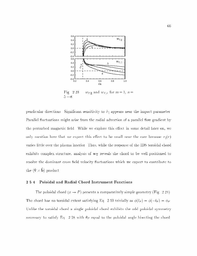
66

0.2 0.4 0.6 0.8 1.0r T

, o-0.4

-0.2

0.0

0.2

0.4

0.6-0.4

-0.2

0.0

0.2

0.4

0.6

5

8

5

8

r/a

wT,||

wT, ∧

Fig. 2.23.| wT;k and wT;^ for m=1, n=5 8.

pendicular directions. Signicant sensitivity to ~vk appears near the impact parameter.

Parallel uctuations might arise from the radial advection of a parallel ow gradient by

the perturbed magnetic eld. While we explore this eect in some detail later on, we

only mention here that we expect this eect to be small near the core because vk(r)

varies little over the plasma interior. Thus, while the response of the IDS toroidal chord

exhibits complex structure, analysis of wT reveals the chord to be well positioned to

resolve the dominant cross eld velocity uctuations which we expect to contribute to

the h~v ~bi product.

2.5.4 Poloidal and Radial Chord Instrument Functions

The poloidal chord (x! P ) presents a comparatively simple geometry (Fig. 2.24).

The chord has no toroidal extent satisfying Eq. 2.59 trivially as (lP ) = (lP ) = P .

Unlike the toroidal chord a single poloidal chord exhibits the odd poloidal symmetry

necessary to satisfy Eq. 2.58 with P equal to the poloidal angle bisecting the chord.

67

0

L

-L

ro.P

θP

l

Fig. 2.24.| Poloidal view.

The projections of the velocity components onto lP are given by,

lP = 0; lP = cos( P ); lP r = sin( P ); (2.75)

where we chose to align lP and at P . Substituting these expressions into Eq. 2.57

we may quickly construct integrals in the form given by Eq. 2.60. The poloidal chord

instrument functions for these integrals are,

wP; = 0; (2.76)

wP; = gP cos(m(P )) cos(P ); (2.77)

wP;r = igP sin(m(P )) sin(P ): (2.78)

In this case the radial weighting of the line of sight,

gP =a

LP

dlPdr

=a r

LP (r2 r2o;P )1

2

; (2.79)

contains a single divergence at the point of tangency to .

Two eects stem from the exclusive projection of lP onto and r (Eq. 2.75).

First, the chord is completely insensitive to toroidal ows of any wavenumber (Eq. 2.76).

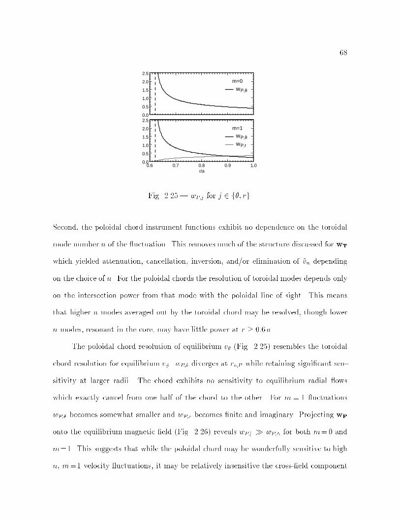
68

0.0

0.5

1.0

1.5

2.0

2.5

0.6 0.7 0.8 0.9 1.0r/a

0.0

0.5

1.0

1.5

2.0

2.5

m=0

wP,θ

wP,θwP,r

m=1

Fig. 2.25.| wP;j for j 2 f; rg.

Second, the poloidal chord instrument functions exhibit no dependence on the toroidal

mode number n of the uctuation. This removes much of the structure discussed for wT

which yielded attenuation, cancellation, inversion, and/or elimination of ~vn depending

on the choice of n. For the poloidal chords the resolution of toroidal modes depends only

on the intersection power from that mode with the poloidal line of sight. This means

that higher n modes averaged out by the toroidal chord may be resolved, though lower

n modes, resonant in the core, may have little power at r 0:6 a.

The poloidal chord resolution of equilibrium v (Fig. 2.25) resembles the toroidal

chord resolution for equilibrium v. wP; diverges at ro;P while retaining signicant sen-

sitivity at larger radii. The chord exhibits no sensitivity to equilibrium radial ows

which exactly cancel from one half of the chord to the other. For m = 1 uctuations

wP; becomes somewhat smaller and wP;r becomes nite and imaginary. Projecting wP

onto the equilibrium magnetic eld (Fig. 2.26) reveals wP;k wP;^ for both m=0 and

m=1. This suggests that while the poloidal chord may be wonderfully sensitive to high

n, m=1 velocity uctuations, it may be relatively insensitive the cross-eld component

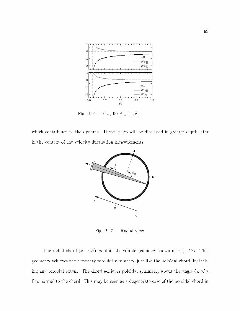
69

0.6 0.7 0.8 0.9 1.0r/a

wP,||

m=1

wP,∧

wP,||

m=0

wP,∧

1

0

-1

-2

1

0

-1

-2

Fig. 2.26.| wP;j for j 2 fk;^g.

which contributes to the dynamo. These issues will be discussed in greater depth later

in the context of the velocity uctuation measurements.

θR

0

L

-L

l

Fig. 2.27.| Radial view.

The radial chord (x ! R) exhibits the simple geometry shown in Fig. 2.27. This

geometry achieves the necessary toroidal symmetry, just like the poloidal chord, by lack-

ing any toroidal extent. The chord achieves poloidal symmetry about the angle R of a

line normal to the chord. This may be seen as a degenerate case of the poloidal chord in

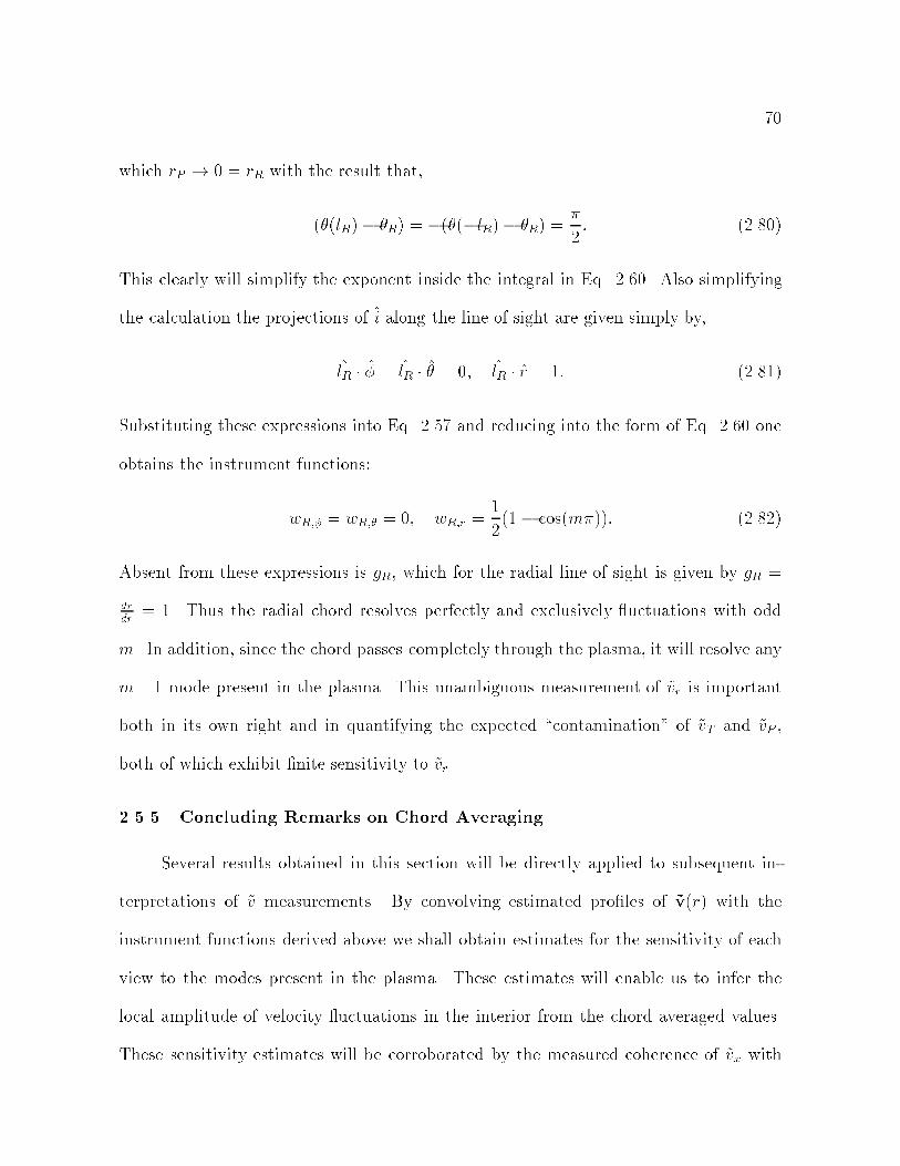
70

which rP ! 0 = rR with the result that,

((lR) R) = ((lR) R) =

2: (2.80)

This clearly will simplify the exponent inside the integral in Eq. 2.60. Also simplifying

the calculation the projections of i along the line of sight are given simply by,

lR = lR = 0; lR r = 1: (2.81)

Substituting these expressions into Eq. 2.57 and reducing into the form of Eq. 2.60 one

obtains the instrument functions:

wR; = wR; = 0; wR;r =1

2(1 cos(m)): (2.82)

Absent from these expressions is gR, which for the radial line of sight is given by gR =

drdr

= 1. Thus the radial chord resolves perfectly and exclusively uctuations with odd

m. In addition, since the chord passes completely through the plasma, it will resolve any

m=1 mode present in the plasma. This unambiguous measurement of ~vr is important

both in its own right and in quantifying the expected \contamination" of ~vT and ~vP ,

both of which exhibit nite sensitivity to ~vr.

2.5.5 Concluding Remarks on Chord Averaging

Several results obtained in this section will be directly applied to subsequent in-

terpretations of ~v measurements. By convolving estimated proles of ~v(r) with the

instrument functions derived above we shall obtain estimates for the sensitivity of each

view to the modes present in the plasma. These estimates will enable us to infer the

local amplitude of velocity uctuations in the interior from the chord averaged values.

These sensitivity estimates will be corroborated by the measured coherence of ~vx with

71

individual magnetic modes. Next, estimates of a at ~v(r) prole will allow mapping of

the relative measured phase between ~b and ~vx to the local h~v ~bi angle in the plasma

interior. Finally, estimates of sensitivity to parallel and cross-eld uctuations will al-

low us to distinguish between uctuations arising from advection and those producing a

dynamo eld.

References

Bendat, J. S. and A. G. Piersol (1980). Engineering Applications of Correlation andSpectral Analysis. New York: John Wiley and Sons.

Bevington, P. R. (1969). Data reduction and error analysis for the physical sciences. NewYork: McGraw-Hill.

Callen, J. D. (1997). Plasma kinetic theory. published class notes for PHYS/NEEP/ECE725.

Carolan, P. G., N. J. Conway, C. A. Bunting, P. Leahy, R. O'Connell, R. Huxford, C. R.Negus, and P. D. Wilcock (1997). Fast charged-coupled device spectrometry usingzoom-wavelength optics. Rev. Sci. Instrum. 68, 10151018.

Carolan, P. G. and R. O'Connell (1995). A multichord spectrometer using an 8 8anode photomultiplier. Rev. Sci. Instrum. 66, 11841188.

Chapman, J. T. and D. J. Den Hartog (1996). Calibration techniques for a fast duo-spectrometer. Rev. Sci. Instrum. 68, 285.

Den Hartog, D. J., A. F. Almagri, and S. C. Prager (1995). Data reduction techniquesfor a fast duo-spectrometer. Rev. Sci. Instrum. 66, 444.

Den Hartog, D. J. and R. J. Fonck (1994). A fast spectroscopic diagnostic for themeasurement of plasma impurity ion dynamics. Rev. Sci. Instrum. 65, 3238.

Evensen, H. T., R. Durst, R. J. Fonck, and S. F. Paul (1995). Optical diagnostic tomeasure ion temperature and parallel velocity uctuations on the tokamak fusiontest reactor. Rev. Sci. Instrum. 66, 845847.

ThornEMI (1993). photomultipliers and accessories. Technical report, Thorn EMI Elec-tron Tubes.

Woehrer, D. (1996). Inversion of impurity proles using the impurity monochromatorarray. PLP-1186.

72

3

Sawtooth Ensemble Analysis

The results presented in the subsequent chapters were achieved over large ensembles of

sawtooth events. The sawtooth represents a discrete manifestation of the dynamo in

the MST. By averaging the sawtooth over a large ensemble we should eectively average

over the ux surface which rotates past our stationary diagnostics. The rst half of this

chapter examines the phenomenology of this cycle, discusses a simple model of sawtooth

behaviour and provides basic denitions critical to sawtooth ensemble analysis. The

second half presents details of the analysis itself, outlining the analysis software and

dening the ensembled quantities.

3.1 Sawtooth Relaxations in MST

3.1.1 The Sawtooth Cycle

The evolution of the total toroidal ux over a shot (Fig. 3.1) is largely determined by

the MST external circuit. The ux rises with the plasma current during the initial portion

of the discharge and soon enters the \ attop" region of the shot which may be maintained

for tens of milliseconds before decaying with the discharge and ultimately terminating

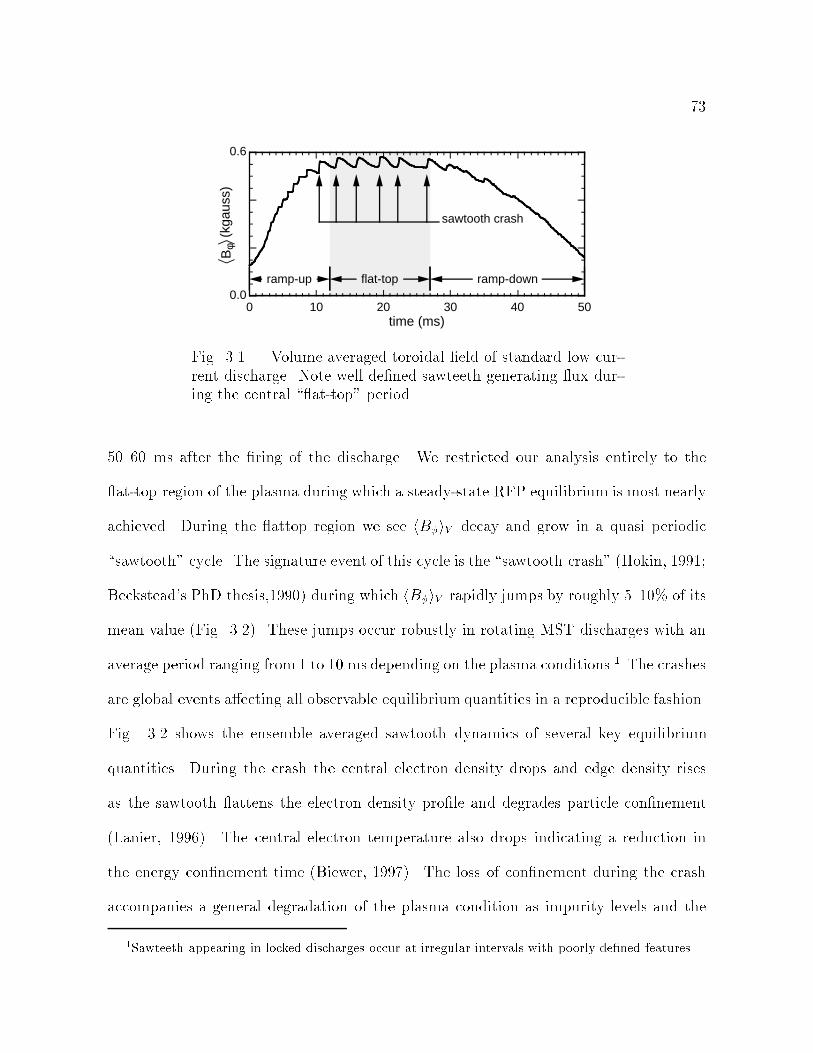
73

0 10 20 30 40 50time (ms)

0.0

0.6

Bφ

(kga

uss)

ramp-up flat-top ramp-down

sawtooth crash

Fig. 3.1.| Volume averaged toroidal eld of standard low cur-rent discharge. Note well dened sawteeth generating ux dur-ing the central \ at-top" period.

5060 ms after the ring of the discharge. We restricted our analysis entirely to the

at-top region of the plasma during which a steady-state RFP equilibrium is most nearly

achieved. During the attop region we see hBiV decay and grow in a quasi periodic

\sawtooth" cycle. The signature event of this cycle is the \sawtooth crash" (Hokin, 1991;

Beckstead's PhD thesis,1990) during which hBiV rapidly jumps by roughly 510% of its

mean value (Fig. 3.2). These jumps occur robustly in rotating MST discharges with an

average period ranging from 1 to 10 ms depending on the plasma conditions.1 The crashes

are global events aecting all observable equilibrium quantities in a reproducible fashion.

Fig. 3.2 shows the ensemble averaged sawtooth dynamics of several key equilibrium

quantities. During the crash the central electron density drops and edge density rises

as the sawtooth attens the electron density prole and degrades particle connement

(Lanier, 1996). The central electron temperature also drops indicating a reduction in

the energy connement time (Biewer, 1997). The loss of connement during the crash

accompanies a general degradation of the plasma condition as impurity levels and the

1Sawteeth appearing in locked discharges occur at irregular intervals with poorly dened features.

74

530

580Bφ (gauss)5.0

6.0

ne 1012/ cm 3( )

-2-1

01

2tim

e (ms)

1.65

1.80-0.35

-0.15

FΘ

-2-1

01

2tim

e (ms)

Fig.

3.2.|Key

equilib

rium

quantities

ensem

bleaveraged

overasaw

toothcycle.

Movingfrom

topto

bottom

:thevolu

meaveraged

toroidaleld

,thelineaveraged

central

electrondensity,

therev

ersalparam

eter,andthepinch

param

eter.

accompanyingrad

iatedpow

erincrease

dram

atically.Twoparam

eterswhich

describ

e

themagn

eticgeom

etryof

theRFPdisch

argealso

evolveover

thecycle.

Thereversal

param

eter,dened

astheratio

oftheedge

toroidaleld

tothevolu

meaveraged

toroidal

eld

(FB (a

)=hB i

V),becom

esdram

aticallymore

negative

durin

gthecrash

before

bein

gpulled

back

closeto

itsorigin

alvalu

e.Thepinch

param

eter,dened

astheratio

of

theedge

poloid

aleld

tothevolu

meaveraged

toroidal

eld

(B (a

)=hB i

V),drop

s

duemostly

totherise

ofhB i

Vin

denom

inator.

Both

eects

re ect

a atten

ingof

the

parallel

curren

tpro

le,(r)

Jk =B

toward

thecon

stantpred

ictedin

Taylor's

model.

Thetoroid

alplasm

acurren

t,Ip=2B

(a)=

o a,rem

ainsrelativ

elycon

stantover

thecycle,

varyingless

than

1%over

thesaw

toothcycle.

Onemodeld

escribestheRFPsaw

toothcycle

asadiscrete

relaxation

ofaresistiv

ely

peak

edcurren

tpro

le(see

forexam

pleOrtlan

iandSchnack

,1993).

Inthismodelthe

equilib

rium,Fig.

3.3,oscillates

with

thesaw

toothaboutacritical

curren

tgrad

ientwith

75

SYSTEM RELAXED

current drive ⇒ Bθ

J || peaks in core

Bφ decays

shear reduced

SYSTEM CRITICAL

instabilities develop

Bθ ⇒ Bφ

J|| flattened

shear restored

DECAY

DYNAMO

τ decay

τ crash

Fig. 3.3.| The sawtooth cycle may be divided into decay and dy-namo phases. In the decay phase the transformer generates poloidal ux while a thermal instability slowly peaks the parallel current onaxis. In the dynamo phase unstable m = 1 tearing modes growrapidly converting poloidal ux into toroidal ux and attening thecurrent prole.

a slow decay phase steepening the gradient and a fast crash phase relaxing it. We shall

describe this cycle starting with the plasma \relaxed" into a minimumenergy state (x 1.1)

characterized by a strong reversal of the toroidal eld in the outer region of the plasma, a

poloidal and toroidal eld of similar peak magnitudes, a parallel current prole which is

relatively at over the inner regions of the plasma, and a safety factor, q(r) rB

RB, which

exhibits strong stabilizing shear. Two easily understood mechanisms drive the system

from this state. First, the toroidal eld, maintained by neither poloidal current drive nor

external coils, dissipates resistively. Second, externally driven toroidal current peaks in

the hot plasma core where the resistivity, T3=2, is lower. Dissipation of this current

further heats the core leading to the thermal instability which slowly peaks the current

prole, driving the discharge from its relaxed state. This decay phase occupies most of

the sawtooth cycle. If unchecked it would lead to the loss of reversal and termination of

76

the RFP discharge in a few ms. However, at a critical gradient in (r) the decay phase

abruptly ends as free energy from the large current gradient drives the rapid growth of

core resistive instabilities. These instabilities relax the plasma back into its minimum

energy state, attening the current prole, enhancing the stabilizing magnetic shear, and

reconnecting poloidal ux into toroidal ux. In addition to the relaxation of the magnetic

geometry, the instabilities induce stochastic eld line transport over the plasma interior

resulting in the observed particle and energy loss. The crash phase of the sawtooth cycle

ends with the plasma returned to its relaxed state. In this model the RFP equilibrium

may be viewed as a complicated oscillation driven about a critical gradient in the current

prole. Thus to obtain a full experimental understanding of dynamo quantities in this

equilibrium we seek to characterize their behavior over this full cycle.

3.1.2 Denition of the Sawtooth Window

To conduct an ensemble over many sawtooth cycles we rst identify the time in

the cycle with which we may align the zero of the ensemble window time axis. For this

purpose we identify the\sawtooth crash time", tc, dened as the point in the sawtooth

cycle at which toroidal ux is generated most rapidly. We locate this point from the

derivative of B which appears as a voltage across the toroidal gap of the MST (Vtg). An

automated sawtooth selection code scans the Vtg for spikes above a preset threshold and

then locates those spikes more precisely through a parabolic t to their local maxima.

The extremely sharp nature of these spikes allows the identication of tc to within a few

s.

In addition to the sawtooth crash time we must determine the interval about tc

which most nearly captures a full sawtooth cycle. This interval may be estimated by

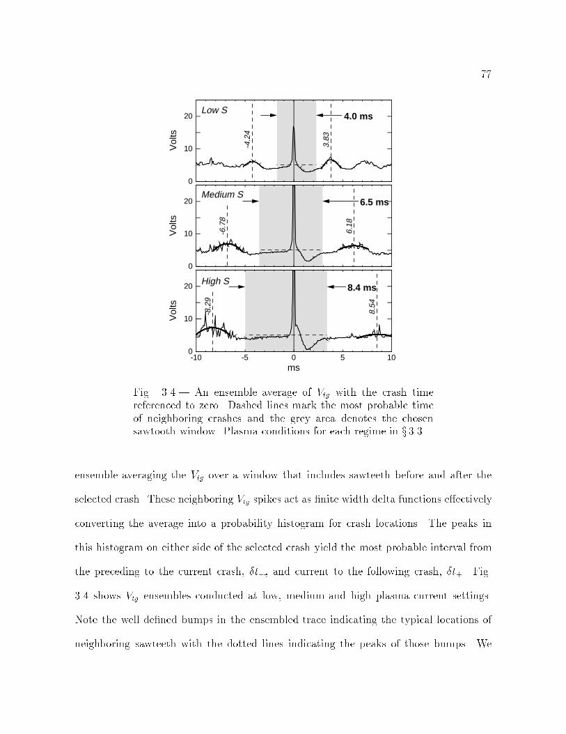
77

1050-5-10ms

Medium S

Low S

High S

6.5 ms

4.0 ms

8.4 ms

6.18

-6.7

8

3.83

-4.2

4

8.54

-8.2

9

20

10

0

Vol

ts

20

10

0

Vol

ts

20

10

0V

olts

Fig. 3.4.| An ensemble average of Vtg with the crash timereferenced to zero. Dashed lines mark the most probable timeof neighboring crashes and the grey area denotes the chosensawtooth window. Plasma conditions for each regime in x 3.3

ensemble averaging the Vtg over a window that includes sawteeth before and after the

selected crash. These neighboring Vtg spikes act as nite width delta functions eectively

converting the average into a probability histogram for crash locations. The peaks in

this histogram on either side of the selected crash yield the most probable interval from

the preceding to the current crash, t, and current to the following crash, t+. Fig.

3.4 shows Vtg ensembles conducted at low, medium and high plasma current settings.

Note the well dened bumps in the ensembled trace indicating the typical locations of

neighboring sawteeth with the dotted lines indicating the peaks of those bumps. We

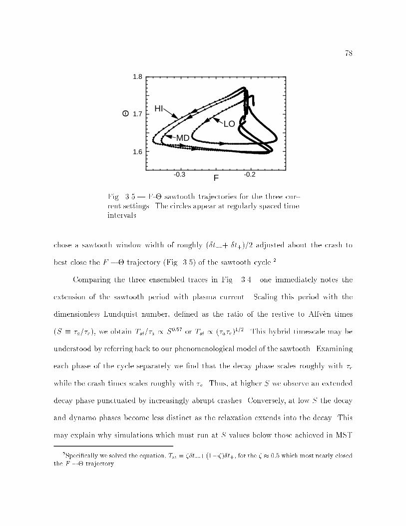
78

1.8

1.7

1.6

-0.3 -0.2

Θ

F

LO

MD

HI

Fig. 3.5.| F- sawtooth trajectories for the three cur-rent settings. The circles appear at regularly spaced timeintervals.

chose a sawtooth window width of roughly (t + t+)=2 adjusted about the crash to

best close the F trajectory (Fig. 3.5) of the sawtooth cycle.2

Comparing the three ensembled traces in Fig. 3.4. one immediately notes the

extension of the sawtooth period with plasma current. Scaling this period with the

dimensionless Lundquist number, dened as the ratio of the restive to Alfven times

(S a=r), we obtain Tst=a / S0:57 or Tst / (ar)1=2. This hybrid timescale may be

understood by referring back to our phenomenological model of the sawtooth. Examining

each phase of the cycle separately we nd that the decay phase scales roughly with r

while the crash times scales roughly with a. Thus, at higher S we observe an extended

decay phase punctuated by increasingly abrupt crashes. Conversely, at low S the decay

and dynamo phases become less distinct as the relaxation extends into the decay. This

may explain why simulations which must run at S values below those achieved in MST

2Specically we solved the equation, Tst = t

+(1)t+, for the 0:5 which most nearly closedthe F trajectory.

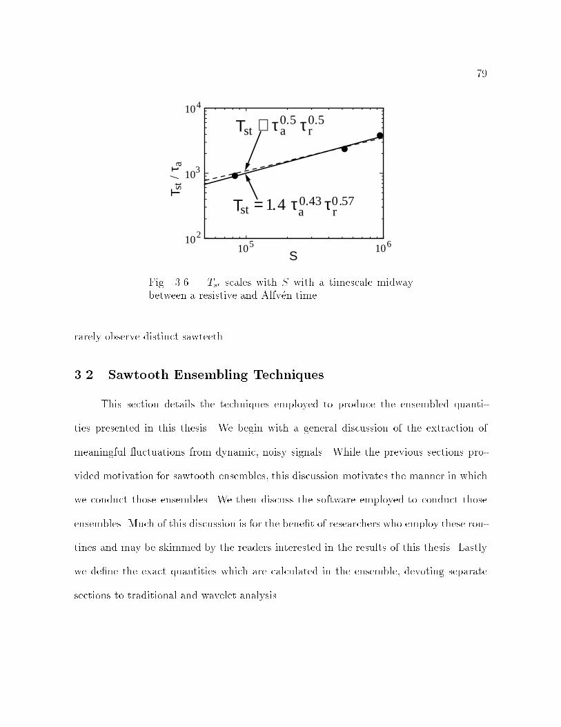
79

Tst = 1.4 τa0.43 τ r

0.57

Tst ∝ τ a0.5 τ r

0.5

102

103

104

106

S105

T st

/τ a

Fig. 3.6.| Tst scales with S with a timescale midwaybetween a resistive and Alfven time.

rarely observe distinct sawteeth

3.2 Sawtooth Ensembling Techniques

This section details the techniques employed to produce the ensembled quanti-

ties presented in this thesis. We begin with a general discussion of the extraction of

meaningful uctuations from dynamic, noisy signals. While the previous sections pro-

vided motivation for sawtooth ensembles, this discussion motivates the manner in which

we conduct those ensembles. We then discuss the software employed to conduct those

ensembles. Much of this discussion is for the benet of researchers who employ these rou-

tines and may be skimmed by the readers interested in the results of this thesis. Lastly

we dene the exact quantities which are calculated in the ensemble, devoting separate

sections to traditional and wavelet analysis.

80

3.2.1 Sawtooth Signal Components

In general we may decompose a signal x(t) windowed about a sawtooth into three

components (Fig. 3.7),

x(t) = xo(t) + ~x(t) +Nx(t); (3.1)

where xo(t) represents the ux-surface averaged or secular evolution of x(t). In the case

of core ion velocity measurements xo(t) describes the deceleration of the uid at the

sawtooth crash. The second term on the RHS of Eq. 3.1, ~x(t), represents uctuations

in x(t). Typically these are spatial uctuations which rotate with the plasma past xed

measurements at Doppler shifted frequencies. For ion velocity measurements this term

contains dynamo uctuations. Finally, Nx(t) represents measurement noise in x(t). In

an ensemble average of x(t) over many sawteeth we assert,

hx(t)i hxo(t)i xo(t); (3.2)

h~x(t)i hNx(t)i 0: (3.3)

This follows our common sense notion that by averaging the sawtooth signals over a

large enough ensemble noise and uctuation will cancel out leaving the average secular

evolution. However the assertion, h~x(t)i 0 rests on equating a ux surface average,

over which MHD uctuations are known to vanish, and an ensemble average. This equiv-

alency holds only if the measured phase of ~x(t) exhibits no preferred value relative to

the sawtooth crash. This may be only approximately true very close to the sawtooth

crash where we occasionally observe magnetic uctuations locking to the lab frame re-

peatedly with the same phase. Unfortunately, these phase locked components of ~x(t)

prove impossible to distinguish from xo(t) with current analysis techniques.

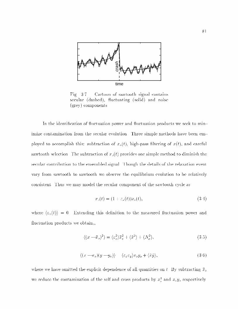
81

time

cras

h

Fig. 3.7.| Cartoon of sawtooth signal containssecular (dashed), uctuating (solid) and noise(grey) components.

In the identication of uctuation power and uctuation products we seek to min-

imize contamination from the secular evolution. Three simple methods have been em-

ployed to accomplish this: subtraction of xo(t), high-pass ltering of x(t), and careful

sawtooth selection. The subtraction of xo(t) provides one simple method to diminish the

secular contribution to the ensembled signal. Though the details of the relaxation event

vary from sawtooth to sawtooth we observe the equilibrium evolution to be relatively

consistent. Thus we may model the secular component of the sawtooth cycle as

xo(t) = (1 + "x(t))xo(t); (3.4)

where h"x(t)i = 0. Extending this denition to the measured uctuation power and

uctuation products we obtain,,

h(x xo)2i = h"2xix2o + h~x2i+ hN2

xi; (3.5)

h(x xo)(y yo)i = h"x"yixoyo + h~x~yi; (3.6)

where we have omitted the explicit dependence of all quantities on t. By subtracting xo

we reduce the contamination of the self and cross products by x2o and xoyo respectively.

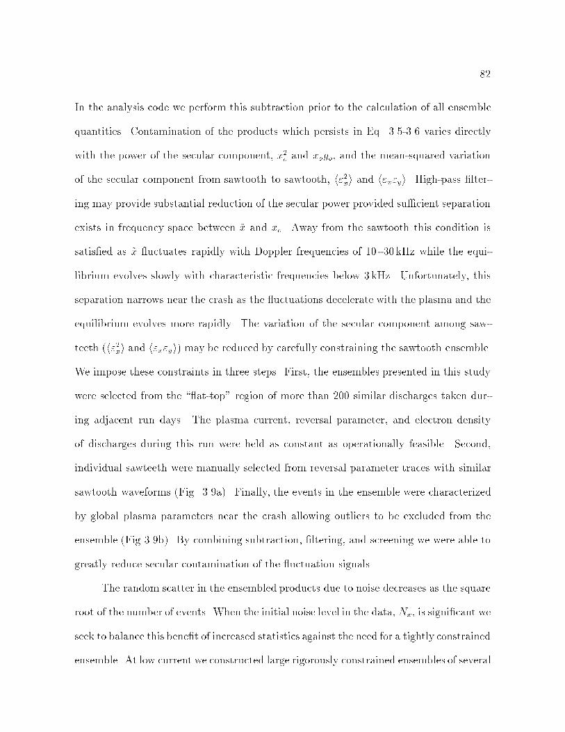
82

In the analysis code we perform this subtraction prior to the calculation of all ensemble

quantities. Contamination of the products which persists in Eq. 3.5-3.6 varies directly

with the power of the secular component, x2o and xoyo, and the mean-squared variation

of the secular component from sawtooth to sawtooth, h"2xi and h"x"yi. High-pass lter-

ing may provide substantial reduction of the secular power provided sucient separation

exists in frequency space between ~x and xo. Away from the sawtooth this condition is

satised as ~x uctuates rapidly with Doppler frequencies of 10 - 30 kHz while the equi-

librium evolves slowly with characteristic frequencies below 3 kHz. Unfortunately, this

separation narrows near the crash as the uctuations decelerate with the plasma and the

equilibrium evolves more rapidly. The variation of the secular component among saw-

teeth (h"2xi and h"x"yi) may be reduced by carefully constraining the sawtooth ensemble.

We impose these constraints in three steps. First, the ensembles presented in this study

were selected from the \ at-top" region of more than 200 similar discharges taken dur-

ing adjacent run days. The plasma current, reversal parameter, and electron density

of discharges during this run were held as constant as operationally feasible. Second,

individual sawteeth were manually selected from reversal parameter traces with similar

sawtooth waveforms (Fig. 3.9a). Finally, the events in the ensemble were characterized

by global plasma parameters near the crash allowing outliers to be excluded from the

ensemble (Fig 3.9b). By combining subtraction, ltering, and screening we were able to

greatly reduce secular contamination of the uctuation signals.

The random scatter in the ensembled products due to noise decreases as the square

root of the number of events. When the initial noise level in the data, Nx, is signicant we

seek to balance this benet of increased statistics against the need for a tightly constrained

ensemble. At low current we constructed large rigorously constrained ensembles of several

83

hundred sawteeth though statistics decreased at higher currents where sawteeth became

both more variable and more widely spaced. While with sucient statistics hNxi ! 0,

the hN2x i term on the RHS of Eq. 3.5 remains. This term amounts to a noise oor

which must be quantied in order to correctly determine the uctuation power h~x2i. If

known, the random error associated with x(t) for each event may be propagated through

the ensemble to determine this oor. However, it is usually more accurate to apply

knowledge of the noise behavior in frequency and time to determine the noise oor of the

ensembled power. This approach is applied later on with considerable success to subtract

a large noise oor from the ensembled IDS signal resolving a comparatively small amount

of velocity uctuation power (x 5.1).

3.2.2 Sawtooth Ensemble Software

The following paragraphs contain a brief overview of the software developed to

analyze signals over a carefully constrained sawtooth ensemble. This code is publicly

available and employed by several researchers for the analysis of widely varying data.

Thus this description serves both to detail the creation and analysis of ensembles pre-

sented in this study, and as a brief introduction to the software for others wishing to

conduct similar studies. Those interested in employing this software are encouraged to

read these comments carefully and to examine the generously commented code found in

[jchapman.public.st corr] and the Appendices of this thesis. On the other hand,

those interested primarily in the measurements presented in this thesis may skim this

description without compromising subsequent comprehension of results.

Sawtooth ensemble analysis proceeds in two basic steps: the generation of an en-

semble and the analysis of signals averaged over that ensemble. A number of routines

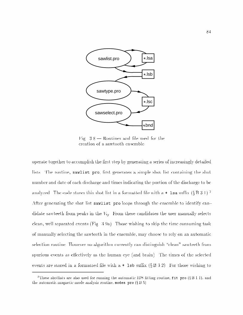
84

.bnd*

.lsa*

.lsb*

sawlist.pro

sawtype.pro

sawselect.pro

.lsc*

Fig. 3.8.| Routines and le used for thecreation of a sawtooth ensemble.

operate together to accomplish the rst step by generating a series of increasingly detailed

lists. The routine, sawlist.pro, rst generates a simple shot list containing the shot

number and date of each discharge and times indicating the portion of the discharge to be

analyzed. The code stores this shot list in a formatted le with a *.lsa sux (xB.3.1).3

After generating the shot list sawlist.pro loops through the ensemble to identify can-

didate sawteeth from peaks in the Vtg. From these candidates the user manually selects

clean, well separated events (Fig. 3.9a). Those wishing to skip the time consuming task

of manually selecting the sawteeth in the ensemble, may choose to rely on an automatic

selection routine. However no algorithm currently can distinguish \clean" sawteeth from

spurious events as eectively as the human eye (and brain). The times of the selected

events are stored in a formatted le with a *.lsb sux (xB.3.2). For those wishing to

3These shotlists are also used for running the automatic IDS tting routine, fit.pro (xB.1.1), andthe automatic magnetic mode analysis routine, modes.pro (xB.5).

85

conduct other types of ensembles the routine triglist.pro generalizes sawlist.pro,

producing *.lsb les with events occurring at regular intervals (i.e. every 5 ms from 10

- 30 ms) or events triggered at times specic to particular experiments (e.g., PPCD re

time).

After creating a sawtooth ensemble with sawlist.pro the user runs a second rou-

tine, sawtype.pro, to characterize each sawtooth by the discharge parameters around

the sawtooth events. In sawtype.pro the user selects the parameters to be \typed" for

a particular ensemble. These parameters may be signals stored in the data base (i.e.

plasma current, electron density, reversal parameter) or signals derived by user dened

routines (i.e. mode frequency). The routine then loops through the events in the *.lsb

le and averages the chosen signals over user dened windows referenced to the individual

sawteeth. The routine stores this information in a third le with a *.lsc sux (xB.3.3)

together with all the sawtooth and shot information contained in the *.lsb le. This

le contains the nal and most complete characterization of the sawtooth ensemble.

After typing the sawtooth list may be \bound" by sawselect.pro to exclude out-

liers and constrain the ensemble. This nal routine produces scatter plots of the typed

quantities and invites the user to dene the upper and lower limits of inclusion (Fig.

3.9b). This process must be approached carefully as careless imposition of limits may

needlessly and drastically reduce the size of the ensemble. For example, excluding 20% of

three uncorrelated quantities will reduce the ensemble by a factor of two. Typically sev-

eral adjustments must be made before the user achieves an appropriate balance between

maintaining sucient statistics in the ensemble and reducing the variance amongst the

included sawtooth events. Once chosen the limits are stored in a separate short le with

a *.bnd sux (xB.3.4). The creation of the *.lsc and *.bnd les completes the rst

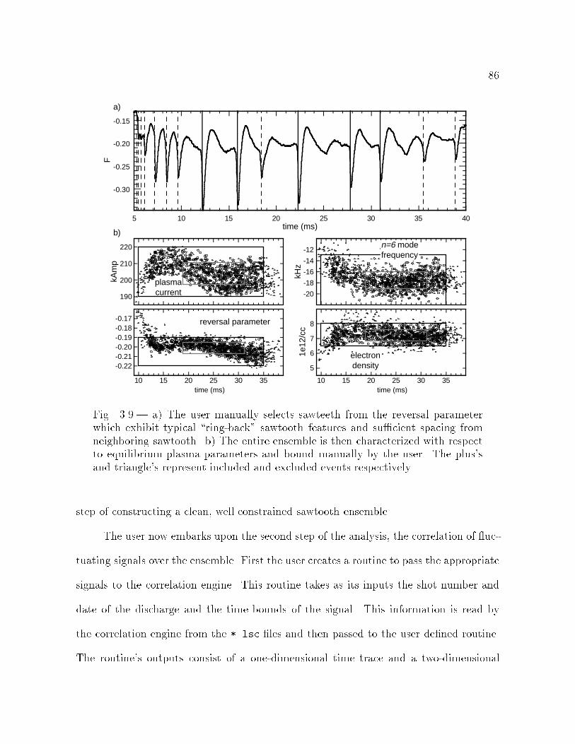
86

-0.15

-0.20

-0.25

-0.30

5 10 15 20 25 30 35 40

F

time (ms)

a)

220

210

200

190

-0.22

-0.20

-0.18-0.17

-0.19

-0.21

-20

-18

-16

-14

-12

8

7

6

5

10 15 20 25 30 35 10 15 20 25 30 35time (ms) time (ms)

plasmacurrent

reversal parameter

n=6 modefrequency

electrondensity

1e12

/cc

kHz

kAm

p

b)

Fig. 3.9.| a) The user manually selects sawteeth from the reversal parameterwhich exhibit typical \ring-back" sawtooth features and sucient spacing fromneighboring sawtooth. b) The entire ensemble is then characterized with respectto equilibrium plasma parameters and bound manually by the user. The plus'sand triangle's represent included and excluded events respectively.

step of constructing a clean, well constrained sawtooth ensemble.

The user now embarks upon the second step of the analysis, the correlation of uc-

tuating signals over the ensemble. First the user creates a routine to pass the appropriate

signals to the correlation engine. This routine takes as its inputs the shot number and

date of the discharge and the time bounds of the signal. This information is read by

the correlation engine from the *.lsc les and then passed to the user dened routine.

The routine's outputs consist of a one-dimensional time trace and a two-dimensional

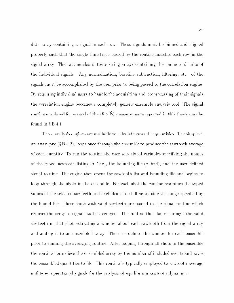
87

data array containing a signal in each row. These signals must be binned and aligned

properly such that the single time trace passed by the routine matches each row in the

signal array. The routine also outputs string arrays containing the names and units of

the individual signals. Any normalization, baseline subtraction, ltering, etc. of the

signals must be accomplished by the user prior to being passed to the correlation engine.

By requiring individual users to handle the acquisition and preprocessing of their signals

the correlation engine becomes a completely generic ensemble analysis tool. The signal

routine employed for several of the h~v ~bi measurements reported in this thesis may be

found in xB.4.1.

Three analysis engines are available to calculate ensemble quantities. The simplest,

st aver.pro (xB.4.2), loops once through the ensemble to produce the sawtooth average

of each quantity. To run the routine the user sets global variables specifying the names

of the typed sawtooth listing (*.lsc), the bounding le (*.bnd), and the user dened

signal routine. The engine then opens the sawtooth list and bounding le and begins to

loop through the shots in the ensemble. For each shot the routine examines the typed

values of the selected sawteeth and excludes those falling outside the range specied by

the bound le. Those shots with valid sawteeth are passed to the signal routine which

returns the array of signals to be averaged. The routine then loops through the valid

sawteeth in that shot extracting a window about each sawtooth from the signal array

and adding it to an ensembled array. The user denes the window for each ensemble

prior to running the averaging routine. After looping through all shots in the ensemble

the routine normalizes the ensembled array by the number of included events and saves

the ensembled quantities to le. This routine is typically employed to sawtooth average

unltered operational signals for the analysis of equilibrium sawtooth dynamics.

88

The two remaining engines, st corr.pro and st wvlt.pro (xB.4.3), operate in an

analogous fashion. However these routines then loop through the ensemble twice. In

the rst loop the calculate the ensemble quantities exactly as in st aver.pro. Then in

the second pass the routines subtract sawtooth averaged quantities from each windowed

signal to extract the uctuating portion of the signal from its secular evolution (Eq. 3.5-

Eq. 3.6). Both routines then ensemble the time resolved products and spectra of every

signal with every other signal. In addition st wvlt.pro ensembles wavelet coecients

dened over both frequency and time. The routine nally calculates the coherence and

phase of the ensembled products and stores all ensembled quantities to le.

3.2.3 Time Series and Fourier Ensemble Analysis

We now turn to the ensembled quantities calculated and stored by the algorithms

outlined above. This section describes the time resolved products and spectra output

by both st corr.pro and st wvlt.pro. A discussion of wavelet analysis ensues in the

following subsection. All the quantities described are stored in generic IDL save les in

a manner described in x ??. We dene xi(t) to be the i'th uctuating signal extending

over a sawtooth window. For every xi(t) we may construct a phase shifted counterpart

pi(t) as,

pi(t) Zdf ei2ftei sgn(f)=2

Zdt0 ei2ft

0

xi(t0)

; (3.7)

where sgn(f) returns the sign of f . In words, pi is obtained from xi by shifting the phase

of its Fourier components by 90o (Ji, 1995). The rst loop of the correlation engine

obtains both hxii and hpii. By subtracting these averages from the individual signals

in the second loop we obtain the uctuating signals, ~xi and ~pi. We now average h~x2i i,

h~xi~xji, and h~xi~pji over the ensemble. These will be referred to respectively as the self,

89

direct, and shifted products. Frequently, the coherence of two signals in time is dened

in signal analysis literature from the self and direct products as,

cij(t) h~xi~xji

(h~x2i ih~x2j i)1

2

: (3.8)

However, cij incorporates both the coherence of the two signals and their relative phase,

cij(t) = ij(t) cos(ij(t)): (3.9)

Here ij(t) is the true coherence of the two signals. This is to say that ij(t) is the

fraction of the power in xi and xj which maintains a non-random phase with respect

to the other signal. This non-random relative phase is then given by ij(t). From Eq.

3.83.9 it is impossible to determine, for example, whether a near zero value of cij arise

from the signals being incoherent or out of phase. We overcome this diculty by using

the shifted product to dene,

sij(t) h~xi~pji

(h~x2i ih~x2j i)1

2

= ij(t) sin(ij(t)): (3.10)

Eqs. 3.83.10 may easily be rearranged to solve for the coherence and phase as,

ij(t) = c 2ij + s 2ij

12 =

h~xi~xji2 + h~xi~pji2h~x2i ih~x2j i

; (3.11)

ij(t) = tan1 sij cij

= tan1

h~xi~pjih~xi~xji

: (3.12)

This technique allows the determination of signal coherence and phase in time much as

it may be dened through spectral analysis in frequency. Extensive simulations have

demonstrated this reliability of the technique and for further assurance we have checked

that ~pi for the cosine component of a spatially resolved magnetic mode matches ~xi for

the sine component of the same mode.

90

The routines st corr.pro and st wvlt.pro apply standard ensemble Fourier anal-

ysis to the signals (e.g. Bendat and Piersol, 1980). Each uctuating signal, ~xi is multi-

plied by a Hanning window to reduce leakage to high frequencies from nite data lengths,

and zero-meaned to remove any DC Fourier component. An FFT of the modied signal

yields the complex Fourier transform Fi. This calculation may be written in continuous

form as,

Fi(f) =

Zdt ei 2 f t (w(t)~xi(t) hw(t)~xi(t)it); (3.13)

where w(t) is the Hanning window. The routine then ensembles the auto-spectral power,

Pii = hFiF i i, and the complex cross-spectral power, Pij = hFiF

j i. The ensembled

spectra are normalized by the number of events and by 1=(hw2it hwi2t ) to account for

the eects of windowing. In addition the routines convert the two sided spectra to one

sided spectra by truncating the redundant negative frequencies and multiplying all but

the DC and Nyquist frequencies by two to preserve uctuation power.4 Coherence and

phase are derived in standard fashion from the ensembled cross spectra as,

ij(f) =

PijP

ij

PiiPjj

1

2

; (3.14)

ij(f) = tan1=(Pij)<(Pij)

: (3.15)

For completely uncorrelated signals the expectation value of ij(f) is given approximately

by 1=pNevent. Though more complicated expressions have been derived simulations and

practical application have indicated that this simple expression provides a robust estimate

of the coherence baseline.

4In IDL the FFT normalization convention yields,P

f Pii =P

t ~x2i=Nt, where Nt is the number

of time points. Dividing Pii by df = 1=(tmax tmin) converts the spectra into the more physicallymeaningful units of power per frequency.

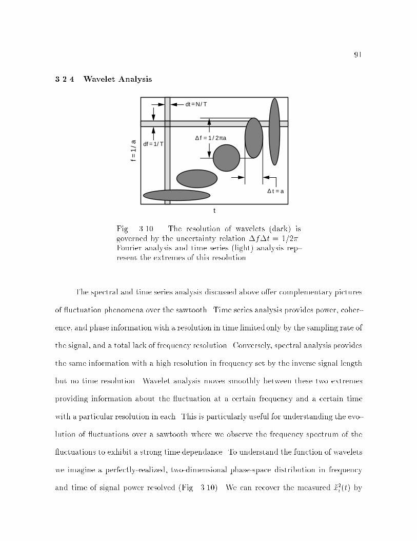
91

3.2.4 Wavelet Analysis

df = 1/ T

dt = N/ T

∆ t = a

∆ f = 1 / 2πa

t

f=1

/a

Fig. 3.10.| The resolution of wavelets (dark) isgoverned by the uncertainty relation ft = 1=2.Fourier analysis and time series (light) analysis rep-resent the extremes of this resolution.

The spectral and time series analysis discussed above oer complementary pictures

of uctuation phenomena over the sawtooth. Time series analysis provides power, coher-

ence, and phase information with a resolution in time limited only by the sampling rate of

the signal, and a total lack of frequency resolution. Conversely, spectral analysis provides

the same information with a high resolution in frequency set by the inverse signal length

but no time resolution. Wavelet analysis moves smoothly between these two extremes

providing information about the uctuation at a certain frequency and a certain time

with a particular resolution in each. This is particularly useful for understanding the evo-

lution of uctuations over a sawtooth where we observe the frequency spectrum of the

uctuations to exhibit a strong time dependance. To understand the function of wavelets

we imagine a perfectly-realized, two-dimensional phase-space distribution in frequency

and time of signal power resolved (Fig. 3.10). We can recover the measured ~x2i (t) by

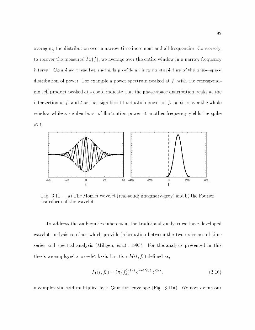
92

averaging the distribution over a narrow time increment and all frequencies. Conversely,

to recover the measured Pii(f), we average over the entire window in a narrow frequency

interval. Combined these two methods provide an incomplete picture of the phase-space

distribution of power. For example a power spectrum peaked at fo with the correspond-

ing self product peaked at t could indicate that the phase-space distribution peaks at the

intersection of fo and t or that signicant uctuation power at fo persists over the whole

window while a sudden burst of uctuation power at another frequency yields the spike

at t.

-4a -2a 0 2a 4at

-4/a -2/a 2/a 4/a0f

Fig. 3.11.| a) The Moirlet wavelet (real-solid; imaginary-grey) and b) the Fouriertransform of the wavelet.

To address the ambiguities inherent in the traditional analysis we have developed

wavelet analysis routines which provide information between the two extremes of time

series and spectral analysis (Miligen, et.al., 1995). For the analysis presented in this

thesis we employed a wavelet basis function M(t; fo) dened as,

M(t; fo) = (=f2o )1=4 et

2f2o =2 ei2t; (3.16)

a complex sinusoid multiplied by a Gaussian envelope (Fig. 3.11a). We now dene our

93

complex wavelet transform coecient through the convolution,

'i(t; fo) =

Zdt0 ~xi(t t0)M(t0; fo): (3.17)

'i(t; fo) contains both the phase and power of the uctuation averaged over a phase-space

region centered around t, fo. The Fourier transform of M(t; fo) (Fig. 3.11b) yields a real

Gaussian centered about fo,

~M (fo; f) /Zdt ei 2 ftM(fo; t) / e2

2(f=fo1)2: (3.18)

Employing the convolution theorem we may equivalently dene 'i(to; fo) as the inverse

Fourier transform of the product of Fi(f) and ~M(fo; f). The ensemble analysis engine,

st wvlt.pro, denes the wavelet coecients in this fashion to reduce computational

time.

By inspection one may see that the resolution of the wavelet packetM(f; t) is given

by the width of its Gaussian envelope, t = 1=fo. Analogously, the resolution of the

wavelet in frequency space is given by the width of ~M(fo; f), f = fo=2. Comparing

the two expressions one discovers that the product of the resolutions is constant yielding

the uncertainty relation,

tf =

1

fo

fo2

=

1

2: (3.19)

Thus, as one increases fo, compressing the wavelet packet to obtain higher time reso-

lution, one increases f , expanding the Gaussian in frequency space to include more

frequencies about fo. The regions resolved in our frequency-time phase space are shown

as ellipses in Fig. 3.10. The uncertainty relation xes the areas of these ellipses prevent-

ing \perfect" resolution of uctuation power distribution in phase space. However, the

94

ability to adjust the position and the relative dimensions of the resolved regions provide

far greater exibility in determining the characteristics of that distribution.

The ensemble code calculates 'i(fo; t) at frequencies unevenly spaced every

f=2. This two-fold redundancy provides smooth contours in frequency and time while

retaining a reasonable degree of computational eciency. The routine then proceeds to

dene ensemble products in direct analogy to the Fourier analysis outlined above. We

dene the wavelet auto and cross spectra as,

Wii(f; t) = h'i(f; t)'i (f; t)i; (3.20)

Wij(f; t) = h'i(f; t)'j(f; t)i: (3.21)

After normalizing the ensembles we then dene the wavelet coherence and phase as,

ij(f; t) =

WijW

ij

WiiWjj

1

2

; (3.22)

ij(f; t) = tan1=(Wij)

<(Wij)

; (3.23)

again in direct analogy to the Fourier analysis.

3.3 Sawtooth Ensembles in this Thesis

The ensembles conducted for this study are listed below along with their operational

parameters. The rst subsection gives the plasma parameters for the ve primary dynamo

runs. These include three runs at low currents and a medium and high current run

which provided the measurements for the Lundquist scaling. The next section describes

the probe scane performed to measure the prole of ~b (x 4.3.1). Finally, we describe

a numerical ensemble conducted with an MHD code at low Lundquist settings. For

the experimental ensembles the MST was run with four banks in standard RFP mode.

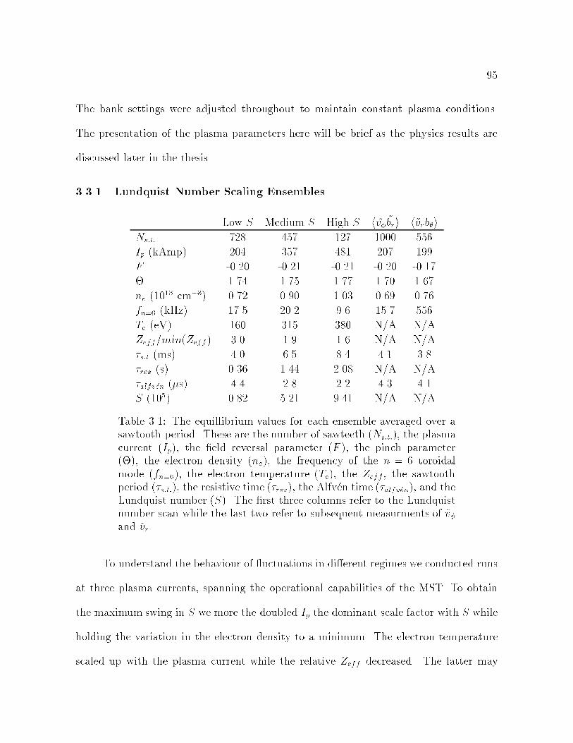
95

The bank settings were adjusted throughout to maintain constant plasma conditions.

The presentation of the plasma parameters here will be brief as the physics results are

discussed later in the thesis.

3.3.1 Lundquist Number Scaling Ensembles

Low S Medium S High S h ~v ~bri h~vrbiNs:t: 728 457 127 1000 556

Ip (kAmp) 204 357 481 207 199

F -0.20 -0.21 -0.21 -0.20 -0.17

1.74 1.75 1.77 1.70 1.67

ne (1013 cm3) 0.72 0.90 1.03 0.69 0.76

fn=6 (kHz) 17.5 20.2 9.6 15.7 556

Te (eV) 160 315 380 N/A N/A

Zeff=min(Zeff ) 3.0 1.9 1.6 N/A N/A

s:t (ms) 4.0 6.5 8.4 4.1 3.8

res (s) 0.36 1.44 2.08 N/A N/A

alfven (s) 4.4 2.8 2.2 4.3 4.1

S (105) 0.82 5.21 9.41 N/A N/A

Table 3.1: The equillibrium values for each ensemble averaged over asawtooth period. These are the number of sawteeth (Ns:t:), the plasmacurrent (Ip), the eld reversal parameter (F ), the pinch parameter(), the electron density (ne), the frequency of the n = 6 toroidalmode (fn=6), the electron temperature (Te), the Zeff , the sawtoothperiod (s:t:), the resistive time (res), the Alfven time (alfven), and theLundquist number (S). The rst three columns refer to the Lundquistnumber scan while the last two refer to subsequent measurments of ~vand ~vr.

To understand the behaviour of uctuations in dierent regimes we conducted runs

at three plasma currents, spanning the operational capabilities of the MST. To obtain

the maximum swing in S we more the doubled Ip the dominant scale factor with S while

holding the variation in the electron density to a minimum. The electron temperature

scaled up with the plasma current while the relative Zeff decreased. The latter may

96

be due to machine conditioning which improved as the run progressed. These settings

produce a three point scaling with over an order of magnitude in S achieved. For the

Lundquist runs we employed one toroidal IDS chord and one poloidal IDS chord. Later

low current runs employed the toroidal chords in the up-down symetric conguration

for a phase resolved measurement of h ~v~b;ni and a radial chord with a toroidal chord

for our measurement of ~vr. Not all supplemental diagnostics were available for the later

low current runs. However, care was taken to match the operational parameters of the

original low current run so we may assume that the unmeasured parameters were fairly

consistent.

3.3.2 Radial Scan of Magnetic Fluctuations

We employed the insertable magnetic probe to conduct a radial scan of ~b(r) for

r 16 cm. To commence the scan we inserted the tip of the boron nitride housing 20 cm

into the MST, aligned the probe with the vacuum B shots, and conditioned the probe

with 40 low current discharges. We then conducted sets of six or more discharges

withdrawing the probe 1 cm from the plasma between each set. We completed a nal

set at a tip insertion of 2 cm, and then reinserted the probe to obtain additional sets

at tip insertions of 20, 19, and 18 cm. This provided a simple check of the early data

against slow evolution of the measured quantities over the run. The sawteeth during

these discharges were irregular and poorly dened due to the degradation of the plasma

by the insertion of the probe, thus we did not pursue sawtooth ensembling for this data.

Instead the signals were ensembled over xed windows during the at-top of the discharge

and then correlated as described in x 3.2.

Fig. 3.12 illustrates some eects of the probe on plasma conditions as a function

97

0.250.20

0.15

0.10

0.050.00

Carbon

0.250.20

0.15

0.10

0.050.00

Radiated Power

Loop Voltage

0

10

20

30

40

n=6 frequency

0

5

10

n=6 locking fraction

0.00.2

0.4

0.6

0.81.0

0 5 10 15 20probe insertion (cm)

210

220

230

0 5 10 15 20probe insertion (cm)

plasma currentkAm

pkH

zauau

Vol

ts

Fig. 3.12.| The plasma sees the magnetic probe as a 0.5 inch-dia boron-nitride lim-iter. At insertions of greater that 10 cm the incidence of locking, impurity radiation,and loop voltage climb.

of insertion depth. At insertions of fewer than 10 cm the probe appears to have little

eect on the plasma condition with impurity radiation levels staying level. However, at

insertions deeper than 10 cm, past the reversal surface, the probe increasingly degrades

the plasma condition. The locking percentage, dened as the percentage of the shot

exhibiting an n = 6 mode frequency with an absolute value less than 3 kHz, climbs

dramatically from zero locking before 10 cm to near total locking at the deepest insertion.

The n=6 mode frequency, averaged over unlocked periods, drops as the probe drags the

plasma. The radiated power grows rapidly with insertion past 10 cm indicating an

increased plasma-probe interaction which is introducing contaminants into the plasma.

At the deepest probe insertion the loop voltage averaged over 30 Volts compared with

20 Volts at shallower insertions. Consequently, the plasma current achieved for the same

capacitor bank settings was substantially reduced. This dramatic contamination of the

98

plasma by the probe at the deeper insertions may introduce signicant and incalculable

errors to the ~b measurements at these radii. However, these eects illustrate the need for

a passive measurement of the dynamo product using non-perturbing edge coils. Indeed,

it is exactly this need which motivates the empirical mapping of ~b(r).

3.3.3 MHD Simulation Ensemble

To compare the empirical results with the predictions of MHD we employed the

nonlinear simulation code named DEBS (Sovinec, 1995).5 This code models an RFP

equilibrium like that obtained in MST although with Lundquist numbers more than an

order of magnitude below those obtained for low current plasmas. For this study we ran

the code at an aspect ratio of three and an S of 103 until the simulation settled into a

stationary equilibrium. We then proceeded to ensemble the Fourier components of the

dominant modes over 100 time slices or realizations to average out transient phenomena.

Analysis of the ensembled self and cross products between these components proceeded

in a manner analagous to that described for actual data.

References

Becksted, J. A. (1995). Sawteeth in the MSTRFP. PhD dissertation, University ofWisconsin Madison, Department of Physics.

Bendat, J. S. and A. G. Piersol (1980). Engineering Applications of Correlation andSpectral Analysis. New York: John Wiley and Sons.

Biewer, T. M. (1997). Electron temperature prole evolution prole a sawtooth in theMSTRFP. PLP-1206.

Hokin, S. and et.al. (1991). Global connement and discrete dynamo activity in theMSTRFP. Phys. Fluids B 3, 2241.

5The DEBS code ensembles presented in this thesis were arranged with and conducted by J. Wright.

99

Ji, H., A. F. Almagri, S. C. Prager, and J. S. Sar (1995). Measurement of the dynamoeect in a plasma. Phys. Plasmas 3(5), 19351942.

Lanier, N. E. (1996). Electron density uctuations associated with tearing mode activity.PLP-1191.

Ortlani, S. and D. D. Schnack (1993). Magnetohydrodynamics of Plasma Relaxation.Singapore: World Scientic.

Sovinec, C. R. (1995). Magnetohydrodynamic simulations of noninductive helicity in-jection in the reversed-eld pinch and tokamak. PhD dissertation, University ofWisconsin Madison, Department of Physics.

van Miligen, B. P., C. Hidalgo, and E. Sanchez (1995). Nonlinear phenomena and inter-mittency in plasma turbulence. Phys. Rev. Lett. 74(3), 395398.

100

4

Magnetic Fluctuations

Fluctuations in the mean magnetic eld of the RFP constitute the better known half

of the h~v ~bi dynamo term. Consequently, full characterization of these uctuations

in time, frequency, wavenumber, and radius proved essential to our measurements. To

accomplish this we performed a radial scan with a magnetic probe, establishing the phase

and amplitude dependence of the three components of ~b(r) roughly a third of the way

into the plasma. At the plasma edge we employed poloidal and toroidal coil arrays to

measure the wavenumber, frequency and time behavior of ~b over the sawtooth crash.

Because of the large radial coherence lengths of these predominantly low-wavenumber

uctuations we were able to combine these measurements to map correlations of ~v with

modes resolved at the edge, to predict behavior of the dynamo product in the core.

Magnetic uctuations have been long studied in the RFP for the role they play in

particle and energy transport, nonlinear three-wave physics, and attening of the current

prole (Hutchinson et.al, 1984; La Haye et.al., 1984; Brotherton-Ratclie, Gimblett, and

Hutchinson, 1987). Thus, many results presented in this chapter are well known and

included because they are essential to subsequent meausurements. The key results of

101

this nature are:

The measured ~br uctuations rise in amplitude away from the edge exceeding the

edge ~b amplitude by a factor of three

The phase of ~br relative to ~b at the wall remains at =2 over the outer third

plasma radius in agreement with MHD which predicts no phase variation over the

full plasma radius.

At the sawtooth crash the total magnetic uctuation power increases tenfold and

the wavenumber dispersion of the power broadens.

The uctuations exhibit Doppler frequencies of 1020 kHz which decrease over the

crash as the plasma decelerates.

The wavenumber dispersion of ~b;n is dominated by the m=1, n=6 mode except

for immediately following the crash when the m=1, n=5 dominates.

In addition we present three additional novel results less critical to the thesis :

Boundary conditions applied to edge measurements of ~b;n and ~b;n imply poloidal

mode numbers of m=0 for n=14, m=1 for n=69, and m2 for n>11.

The relative phase of magnetic coils in the poloidal array exhibits a poloidal de-

pendence consistent with the outward shift of the resonant ux surface.

The magnitude of ~b averaged over the sawtooth cycle scales weakly with S, with

most of the scaling stemming from the decreased duty of the uctuations at high

S.

We structure this chapter in three sections. The rst section brie y describes the

magnetic probe and coil arrays employed for our measurements. Next we establish sign

conventions for the description of the uctuations consistent with the observed pertur-

bation structure and apply boundary conditions to determine the behavior of ~b at the

edge. Finally, we present the results listed above starting with the key probe and the coil

arrays measurements and ending with short sections describing the three new results.

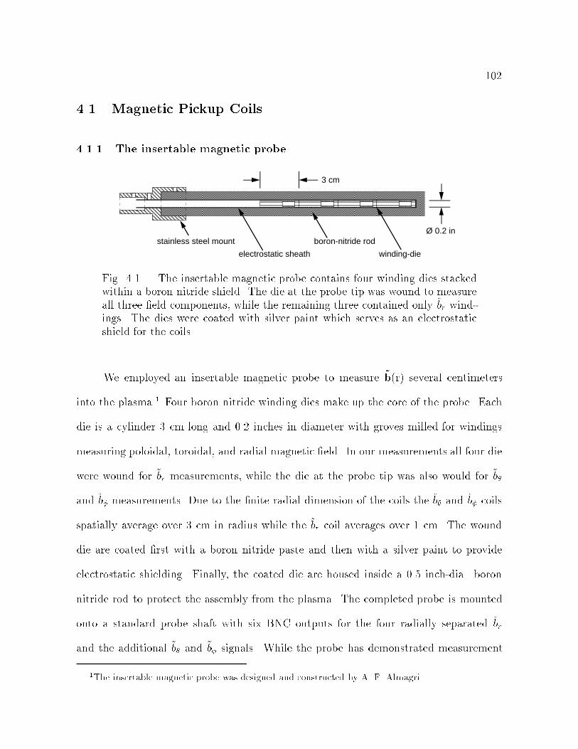
102

4.1 Magnetic Pickup Coils

4.1.1 The insertable magnetic probe

stainless steel mount boron-nitride rod

electrostatic sheath winding-die

3 cm

Ø 0.2 in

Fig. 4.1.| The insertable magnetic probe contains four winding dies stackedwithin a boron nitride shield. The die at the probe tip was wound to measureall three eld components, while the remaining three contained only ~br wind-ings. The dies were coated with silver paint which serves as an electrostaticshield for the coils.

We employed an insertable magnetic probe to measure ~b(r) several centimeters

into the plasma.1 Four boron nitride winding dies make up the core of the probe. Each

die is a cylinder 3 cm long and 0.2 inches in diameter with groves milled for windings

measuring poloidal, toroidal, and radial magnetic eld. In our measurements all four die

were wound for ~br measurements, while the die at the probe tip was also would for ~b

and ~b measurements. Due to the nite radial dimension of the coils the ~b and ~b coils

spatially average over 3 cm in radius while the ~br coil averages over 1 cm. The wound

die are coated rst with a boron nitride paste and then with a silver paint to provide

electrostatic shielding. Finally, the coated die are housed inside a 0.5 inch-dia. boron

nitride rod to protect the assembly from the plasma. The completed probe is mounted

onto a standard probe shaft with six BNC outputs for the four radially separated ~br

and the additional ~b and ~b signals. While the probe has demonstrated measurement

1The insertable magnetic probe was designed and constructed by A. F. Almagri.

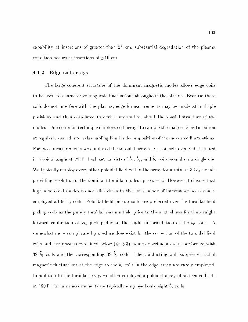
103

capability at insertions of greater than 25 cm, substantial degradation of the plasma

condition occurs at insertions of >10 cm.

4.1.2 Edge coil arrays

The large coherent structure of the dominant magnetic modes allows edge coils

to be used to characterize magnetic uctuations throughout the plasma. Because these

coils do not interfere with the plasma, edge ~b measurements may be made at multiple

positions and then correlated to derive information about the spatial structure of the

modes. One common technique employs coil arrays to sample the magnetic perturbation

at regularly spaced intervals enabling Fourier decomposition of the measured uctuations.

For most measurements we employed the toroidal array of 64 coil sets evenly distributed

in toroidal angle at 241P. Each set consists of ~b, ~b, and ~br coils wound on a single die.

We typically employ every other poloidal eld coil in the array for a total of 32 ~b signals

providing resolution of the dominant toroidal modes up to n=15. However, to insure that

high n toroidal modes do not alias down to the low n mode of interest we occasionally

employed all 64 ~b coils. Poloidal eld pickup coils are preferred over the toroidal eld

pickup coils as the purely toroidal vacuum eld prior to the shot allows for the straight

forward calibration of B pickup due to the slight misorientation of the ~b coils. A

somewhat more complicated procedure does exist for the correction of the toroidal eld

coils and, for reasons explained below (x 4.3.3), some experiments were performed with

32 ~b coils and the corresponding 32 ~b coils. The conducting wall suppresses radial

magnetic uctuations at the edge so the ~br coils in the edge array are rarely employed.

In addition to the toroidal array, we often employed a poloidal array of sixteen coil sets

at 180T. For our measurements we typically employed only eight ~b coils.

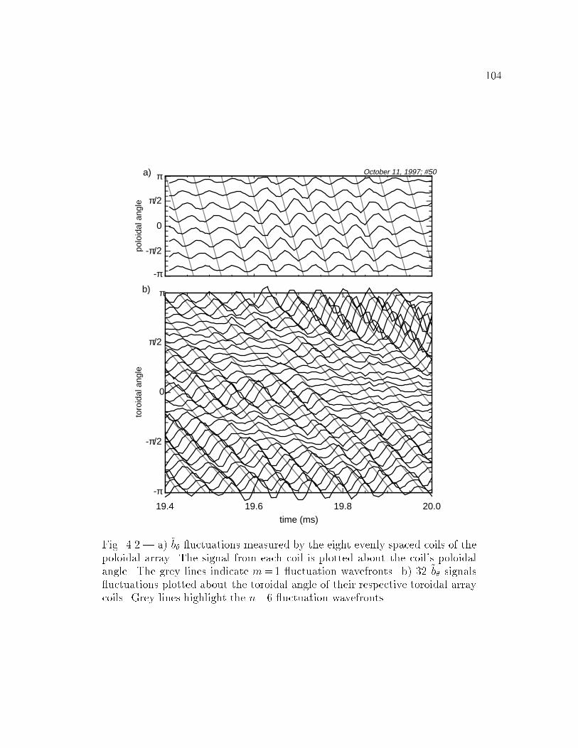
104

October 11, 1997; #50

π

π/2

0

-π/2

-π

b)

19.4 19.6 19.8 20.0time (ms)

a) π

π/2

0

-π/2

-π

polo

idal

ang

leto

roid

al a

ngle

Fig. 4.2.| a) ~b uctuations measured by the eight evenly spaced coils of thepoloidal array. The signal from each coil is plotted about the coil's poloidalangle. The grey lines indicate m=1 uctuation wavefronts. b) 32 ~b signals uctuations plotted about the toroidal angle of their respective toroidal arraycoils. Grey lines highlight the n=6 uctuation wavefronts.

105

To resolve magnetic modes with amplitudes just a few percent the mean eld the

relative gains of coils in the toroidal array must be extremely well calibrated. Though

coil areas were measured upon the installation of the arrays, uncertainties in that initial

calibration, slight errors in the coil orientations, and the accumulated integrator drift

combine to produce substantial errors in the recorded coil gains. These errors dominate

the actual magnetic uctuations such that Fourier analysis of coils normalized with the

recorded gains yields the locked mode structure of the calibration errors. To overcome

this diculty we employ the toroidal symmetry of the magnetic eld averaged over a time

window which greatly exceeds the uctuation period, to perform an in situ calibration of

the coil gains. This technique has proven extremely eective, even enabling the resolution

of the locked mode structure by calibrating the gains over an average of several shots.

Because of the substantial poloidal asymmetry in the mean eld the same technique

may not be used to normalize the poloidal array signals. This generally prevents the

straight-forward application of poloidal mode analysis with the poloidal array signals.

4.1.3 Standard Fourier analysis of edge magnetics

We employ standard spatial Fourier decomposition to extract the uctuating com-

ponents of individual toroidal modes from the toroidal array signal. We dene the time

varying cosine, ~b;n(t), and sine, ~b;n(t), amplitude of the n'th toroidal modes simply as,

~b;n(t) 2

Nc

Xi

~b cos(ni) = b;nei(mc+!t+bn); (4.1)

~b;n(t) 2

Nc

Xi

~b sin(ni) = b;nei(mc+!t+bn+

2); (4.2)

where i is the toroidal angle of the i'th coil, and c is the poloidal angle of the array.

In principle we should include high n aliased modes (n0 = kNc n; k 2 f1; 2; 3; : : : g),

106

however, in practice ifNc is large enough the aliased power should be minimal. Physically,

~b;n may be interpreted as the instantaneous amplitude of the n'th toroidal mode at = 0,

= c while ~b;n(t) is the amplitude of that same mode at = =2n, = c. The codes

which perform the normalization and Fourier analysis of the toroidal array signals may

be found in xB.5.

4.2 Fluctuation Geometry and Boundary Conditions

The dominant magnetic modes in MSTmay be viewed as standing waves which vary

harmonically in and but not in r. These modes travel with the plasma past stationary

coils in the lab frame at Doppler frequencies of 1020 kHz while the amplitude of the

modes in the plasma frame evolves on the time scales of the sawtooth cycle. Correlation

with these global magnetic uctuations requires consistent denitions of the uctuation

geometry and propagation direction. We specify these below, establishing conventions

consistent with the observed uctuations which will be employed for the remainder of

this thesis. We also derive simple relations between the individual components of ~b from

the edge boundary conditions in MST. We employ the right-handed toroidal geometry

shown in Fig. 4.3 and its cylindrical analog for these calculations and throughout the

remainder of this thesis.

4.2.1 The sign of m and n

In the RFP most of the uctuation power resides in a few m=1, n > 2R=a modes

resonant near the core and them=0, n=1 mode resonant at the reversal surface (x 4.3.2).

We determine the relative signs of m and n for a single core mode from the resonance

107

zRr

Bθ

Bφ Eφ

φθ

Fig. 4.3.| A right-handed toroidal geometry is employed consis-tently throughout this thesis. Note the direction of is oppositethat of the MST naming convention. Cylindrical calculationsemploy an analogous geometry.

condition,

kmn B =m

rB +

n

RB = 0; (4.3)

yielding,

m

n= rB

RB> 0; (4.4)

where the nal inequality derives from the negative ratio of B and B in the core (Fig.

4.3). Eq. 4.4 provides the orientation of kmn, however the wavenumber's sign depends

on the propagation direction of the perturbations. This may be obtained by inspection of

the magnetic uctuations wavefronts measured by the poloidal and toroidal arrays (Fig.

4.2). The slopes of these wavefronts is consistent with m=1, n > 0, and ! > 0 where the

equation for the wavefront is given by, m+ n+!t = cons. We may also take the time

derivative of the wavefront equation obtaining the Doppler frequency of the perturbation,

mv=r+nv=R+! = 0. With ! > 0 and n > 0, assuming nv=R mv=r, this relation

mandates that the toroidal velocity of the modes be negative, v < 0, in agreement with

the measured ion ow in the MST core.

108

Plasma

ConductingWall

Vacuum Region

Limiter

Fig. 4.4.| Graphite limiters create a thin 1 cm vacuum regionbetween the plasma and the 5 cm thick aluminum shell.

The determination of the uctuation geometry allows us to correlate spatially sepa-

rated uctuation measurements provided they share the mode structure of the dominant

magnetic uctuations. The phase measured between two single helicity signals, ~x and ~y

would be given by,

(~x; ~y) = m(x y) + n(x y) + x y; (4.5)

where x(y) and x(y) are the poloidal and toroidal locations of the ~x(~y) measurements,

and x y is the relative phase of the uctuations at the same location in the plasma.

We typically wish to solve for this relative phase shift, subtracting o the phase incurred

from the physical separation of the measurements,

x y = (~x; ~y)m(x y) n(x y): (4.6)

Throughout this thesis the term \local phase" will refer to the term on the LHS of Eq.

4.6.

109

4.2.2 Edge Boundary Conditions

Conducting wall and thin vacuum region

The boundary conditions at the edge of the plasma determine the relative phase and

amplitude of ~br, ~b, and ~b at r= a. A highly conductive aluminum shell surrounds the

MST plasma suppressing the growth of linear tearing modes and inductively canceling

fast radial magnetic eld uctuations at the edge. The resistive shell time is on the

order of one second while, for a rotating plasma, the tearing modes typically uctuate at

1020 kHz. Thus to the dominant uctuations the MST wall looks perfectly conducting

allowing us to stipulate our rst boundary condition,

~br(a; ) = 0: (4.7)

This condition fails to hold at gaps in the shell which extend about the machine in the

toroidal and poloidal direction. Sizable radial eld errors grow robustly at the gaps

providing a stationary reference frame to which the plasma can lock. However, the

discharges chosen for our measurements rotated rapidly past these errors providing to

good approximation a symmetric conducting outer boundary. The aluminum MST shell

serves also as the vacuum chamber allowing in principle formation of plasma up to the

shell wall. However, graphite limiters which protrude approximately 1 cm from the wall

prevent this, forming a thin vacuum region about the plasma. This region insulates the

plasma from the wall allowing us to stipulate our second boundary condition,

~jr(a; ) = 0: (4.8)

Like Eq. 4.7, this condition breaks down at the toroidal gap and poloidal gap. However,

for the rotating discharges selected for our measurements Eq. 4.8 is observed to hold.

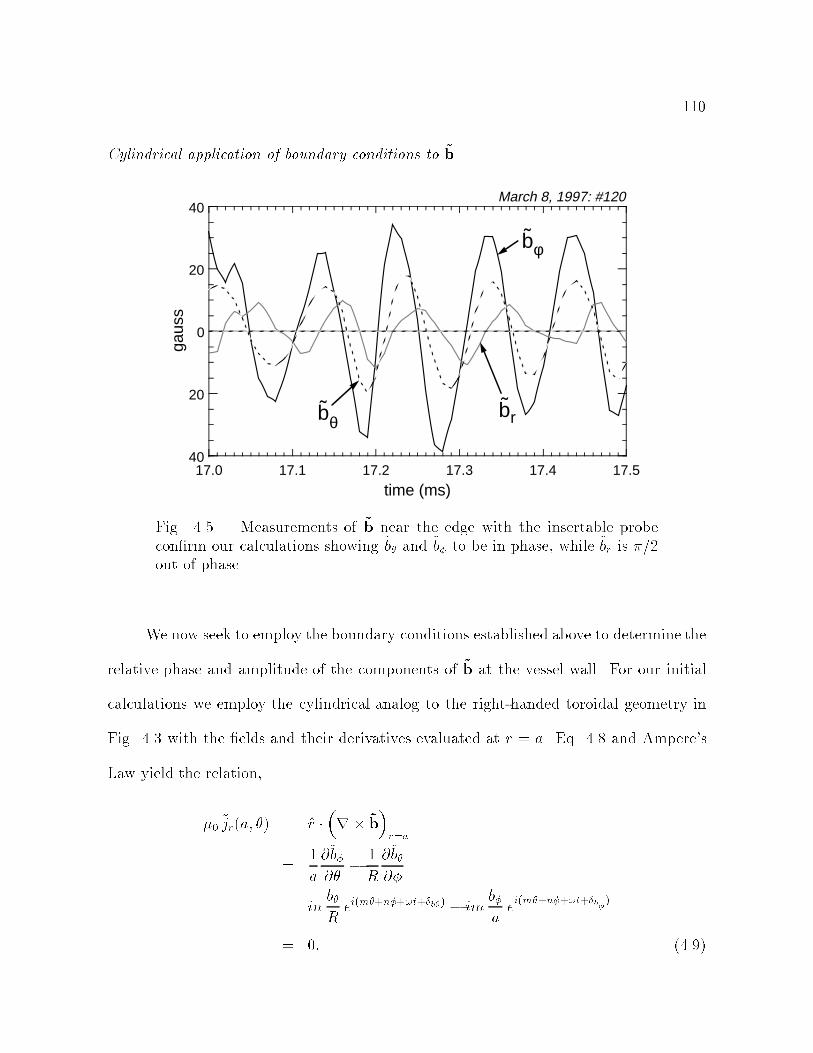
110

Cylindrical application of boundary conditions to ~b

bθ

bφ

br

40

20

0

20

40

time (ms)

gaus

sMarch 8, 1997: #120

17.0 17.3 17.4 17.517.217.1

Fig. 4.5.| Measurements of ~b near the edge with the insertable probeconrm our calculations showing ~b and ~b to be in phase, while ~br is /2out of phase.

We now seek to employ the boundary conditions established above to determine the

relative phase and amplitude of the components of ~b at the vessel wall. For our initial

calculations we employ the cylindrical analog to the right-handed toroidal geometry in

Fig. 4.3 with the elds and their derivatives evaluated at r = a. Eq. 4.8 and Ampere's

Law yield the relation,

0 ~jr(a; ) = r r ~b

r=a

=1

a

@~b@

1

R

@~b@

= inbRei(m+n+!t+b) im

baei(m+n+!t+b )

= 0: (4.9)

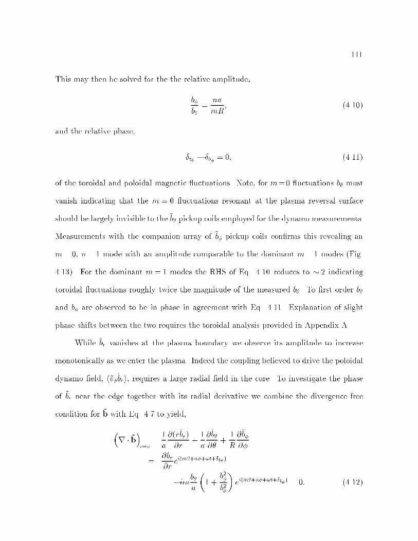
111

This may then be solved for the the relative amplitude,

bb

=na

mR; (4.10)

and the relative phase,

b b = 0; (4.11)

of the toroidal and poloidal magnetic uctuations. Note, for m=0 uctuations b must

vanish indicating that the m = 0 uctuations resonant at the plasma reversal surface

should be largely invisible to the ~b pickup coils employed for the dynamo measurements.

Measurements with the companion array of ~b pickup coils conrms this revealing an

m= 0, n= 1 mode with an amplitude comparable to the dominant m= 1 modes (Fig.

4.13). For the dominant m= 1 modes the RHS of Eq. 4.10 reduces to 2 indicating

toroidal uctuations roughly twice the magnitude of the measured b. To rst order b

and b are observed to be in phase in agreement with Eq. 4.11. Explanation of slight

phase shifts between the two requires the toroidal analysis provided in Appendix A.

While ~br vanishes at the plasma boundary we observe its amplitude to increase

monotonically as we enter the plasma. Indeed the coupling believed to drive the poloidal

dynamo eld, h~v~bri, requires a large radial eld in the core. To investigate the phase

of ~br near the edge together with its radial derivative we combine the divergence free

condition for ~b with Eq. 4.7 to yield,

r ~b

r=a=

1

a

@(r~br)

@r+1

a

@~b@

+1

R

@~b@

=@br@r

ei(m+n+!t+br )

imba

1 +

b2b2

ei(m+n+!t+b ) = 0: (4.12)

112

With some manipulation, Eq. 4.12 yields the relations,

a

b

@br@r

= m

1 +

b2b2

: (4.13)

and,

~b ~br =

2; (4.14)

For the dominant m=1, tearing modes Eq. 4.13 indicates a large growth of ~br from its

zero value at the edge. The =2 phase shift predicted by Eq. 4.14 is observed with minor

corrections which may also be explained through the toroidal analysis in Appendix A.

4.3 Magnetic Fluctuation Measurements

Below we describe the results from a number of measurements which provide a

fairly complete characterization of the magnetic uctuations in MST. We begin with

the measured radial prole of the amplitude and phase of the individual components of

~b(r). We then describe the behavior of individual toroidal modes resolved by the edge coil

arrays. Both of these measurements provide essential background for subsequent analysis

of both measured velocity uctuations and dynamo products. The last three sections

contain novel results which are, however, less critical to this thesis. First we dene and

describe the measured behavior of \average m" for the resolved toroidal modes. We then

report the manifestation of toroidal eects in the phase of ~b as a function of poloidal

angle. And lastly, we present scaling results of the magnetic uctuations with Lundquist

number.

113

4.3.1 Measured magnetic uctuation proles

From boundary conditions imposed on the plasma at the edge we were able to derive

the relative phase and amplitude of the three components of ~b. However, moving into

the plasma these relations change as ~br and ~jr both become non-zero. Our measurement

of the dynamo product relies on the estimation of the amplitude and phase of magnetic

uctuations in the interior of the plasma from measurements of ~b;n at the edge. This

motivated the measurements with the magnetic probe of the uctuations over 15 cm into

the plasma. The details of the experimental run may be found in x 3.3.2 and the probe

is described above in x 4.1.1. Below we present the proles predicted by MHD and then

compare those proles to measurements of the uctuation amplitude and phase. We nd

that within the range of the probe scan all components of ~b increase away from the wall

with a relative phase which does not vary. The passing of ~b and ~b through zero as

predicted by MHD was not observed.

MHD predictions

The uctuation proles predicted by MHD are shown for each component of ~b(r)

in Fig. 4.6. MHD predicts ~br to grow to roughly three times ~b(a) in the plasma mid

region while ~b rises sharply from the edge and then passes through zero near the deepest

insertion of the uctuation scan. ~b rises more gradually and then turns over mid-radius,

passing through zero deep into the plasma. The simulation holds ~b and ~br to identical

values in core and sets ~b(0) = 0. Other than phase shifts which occur when the

amplitudes pass through zero the uctuations maintain a relative phase over the plasma

which does not vary from that set by the boundary conditions at the edge.

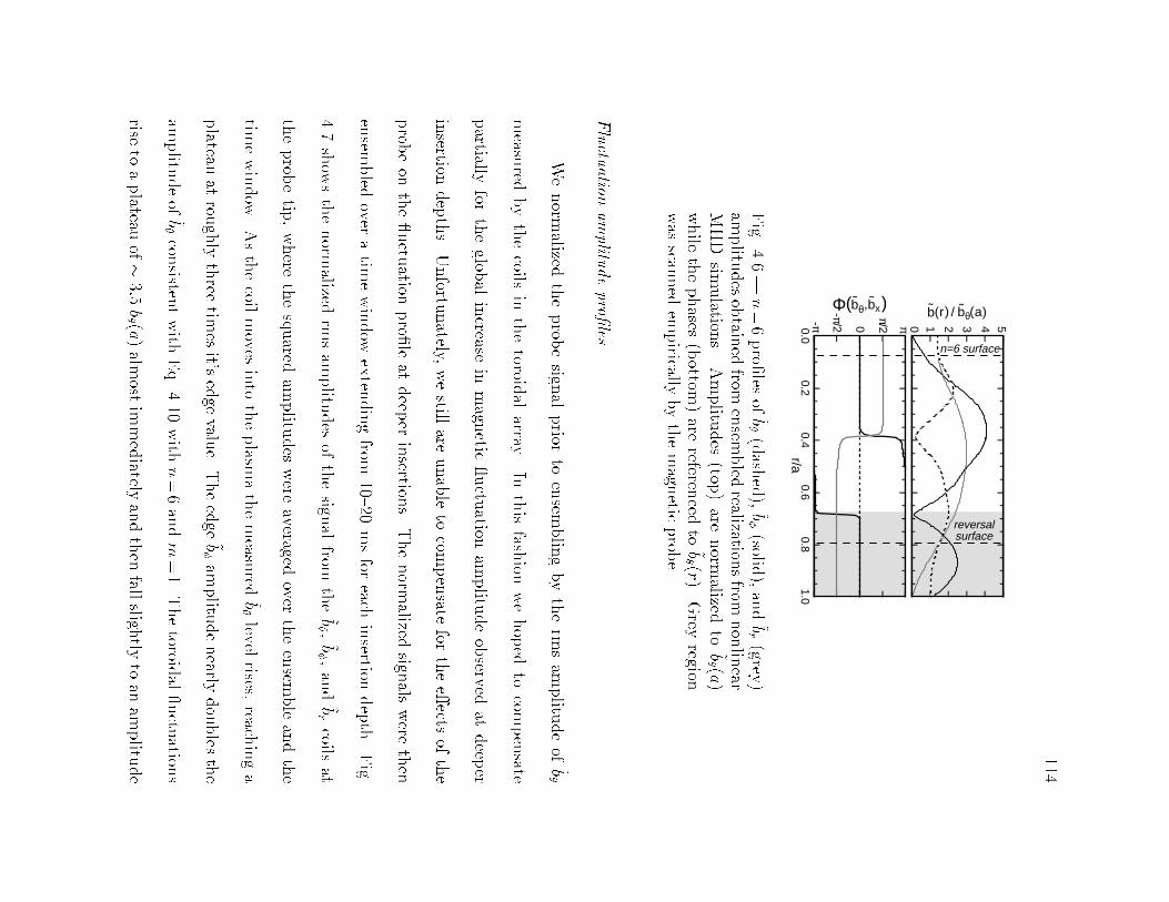
114

0.00.2

0.40.6

0.81.0

543210-π

-π/2 0

π/2 π

r/a

b(r) / bθ(a)Φ(bθ,bx)

n=6 surface

reversalsurface

Fig.

4.6.|n=6pro

lesof~b(dash

ed),~b(solid

),and~br(grey

)am

plitu

desobtain

edfrom

ensem

bled

realizationsfrom

nonlinear

MHD

simulation

s.Amplitu

des

(top)are

norm

alizedto

~b (a

)

while

thephases

(bottom

)are

referenced

to~b (r).

Grey

regionwas

scanned

empirically

bythemagn

eticprob

e.

Fluctu

ationam

plitude

proles

Wenorm

alizedtheprob

esign

alprior

toensem

blingbytherm

sam

plitu

deof

~b

measu

redbythecoils

inthetoroid

alarray.

Inthisfash

ionwehoped

tocom

pensate

partially

fortheglob

alincrease

inmagn

etic uctu

ationam

plitu

deobserved

atdeep

er

insertion

depths.

Unfortu

nately,

westill

areunableto

compensate

fortheeects

ofthe

prob

eon

the uctu

ationpro

leat

deep

erinsertion

s.Thenorm

alizedsign

alswere

then

ensem

bled

overatim

ewindow

exten

dingfrom

1020msfor

eachinsertion

depth.Fig.

4.7show

sthenorm

alizedrm

sam

plitu

des

ofthesign

alfrom

the~b ,~b ,

and~brcoils

at

theprob

etip

,where

thesquared

amplitu

des

were

averagedover

theensem

bleandthe

timewindow

.Asthecoil

moves

into

theplasm

athemeasu

red~blevel

rises,reach

inga

plateau

atrou

ghlythree

timesit's

edge

value.

Theedge

~bam

plitu

denearly

doubles

the

amplitu

deof~bcon

sistentwith

Eq.4.10

with

n=6andm=1.

Thetoroid

al uctu

ations

riseto

aplateau

of3:5

b (a

)alm

ostim

mediately

andthen

fallsligh

tlyto

anam

plitu

de

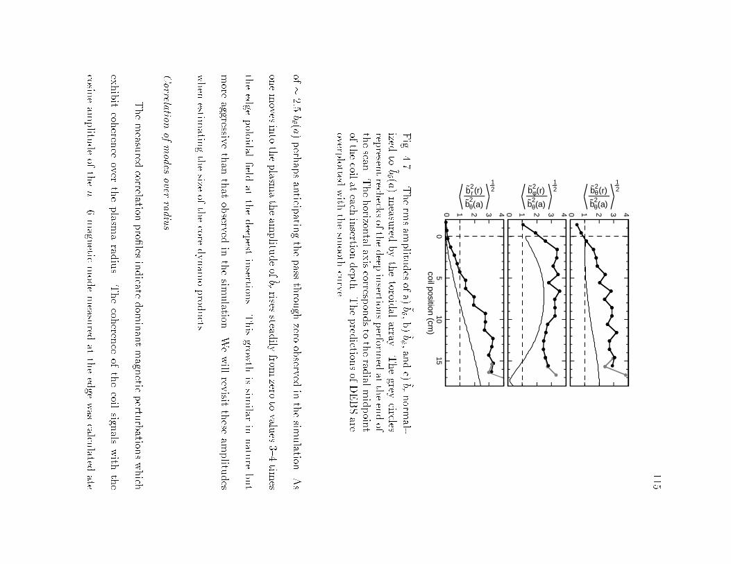
115

05

1015

coil position (cm)

0 1 2 3 40 1 2 3 40 1 2 3 4

θb2(r)

bθ2(a)

12φb2(r)

bθ2(a)

12

rb2(r)

bθ2(a)

12

Fig.

4.7.|Therm

sam

plitu

desofa)~b ,b)~b ,andc)~brnorm

al-

izedto

~b (a

)measu

redbythetoroid

alarray.

Thegrey

circlesrep

resentrech

ecksofthedeep

insertion

sperform

edat

theendof

thescan

.Thehorizon

talaxiscorresp

ondsto

therad

ialmidpoin

tofthecoil

ateach

insertion

depth.Thepred

ictionsofDEBSare

overplotted

with

thesm

oothcurve.

of2:5

b (a

)perh

apsanticip

atingthepass

throu

ghzero

observed

inthesim

ulation

.As

onemoves

into

theplasm

atheam

plitu

deof~brrises

steadily

fromzero

tovalu

es34

times

theedge

poloid

aleld

atthedeep

estinsertion

s.Thisgrow

thissim

ilarin

natu

rebut

more

aggressivethan

that

observ

edin

thesim

ulation

.Wewill

revisit

these

amplitu

des

when

estimatin

gthesize

ofthecore

dynam

oprod

ucts.

Correlation

ofmodes

overradiu

s

Themeasu

redcorrelation

pro

lesindicate

dom

inantmagn

eticpertu

rbation

swhich

exhibitcoh

erence

overtheplasm

arad

ius.

Thecoh

erence

ofthecoil

signals

with

the

cosineam

plitu

deof

then=6magn

eticmodemeasu

redat

theedge

was

calculated

ate

116

05

1015

coil position (cm)

0.00.2

0.4

0.6

0.81.0

0.00.2

0.4

0.6

0.81.0

0.00.2

0.4

0.6

0.81.0

γ bθ,n=6(a) ,br

(r )( ) γ bθ,n=6(a) ,bφ

(r )( ) γ bθ,n=6(a) , bθ

(r)( )

Fig.

4.8.|Thecorrelation

ofthemeasu

red~bwith

~b;n=

6mea-

sured

atthewall.

Thecorrelation

baselin

eisless

than

5%.

eachinsertion

.Thepoloid

al uctu

ationsexhibitacoh

erence

of0.5

with

then=6

modeover

theentire

regionscan

ned

bytheprob

e.Thissubstan

tialcoh

erence

re ects

not

only

theglob

alnatu

reof

then=6pertu

rbation

butits

dom

inance

ofthetoroid

al

modedisp

ersion.Thecoh

erence

forthetoroid

alandrad

ial uctu

ationsissom

ewhat

lower

though

stillwell

above

thecoh

erence

baselin

e.Thecoh

erence

levels

forthese

two

componentsappears

todrop

osligh

tlyat

thedeep

estinsertion

s.How

everthisdrop

also

occurs

inthethree

radial

coilsspaced

atshallow

erinsertion

sandmay

therefore

bean

artifactoftheprob

e-plasm

ainteraction

.Even

so,~brexhibits

acoh

erence

of0.2

atthe

deep

estinsertion

s,onlysligh

tlybelow

itsvalu

eat

thewall.

Thus,wemay

feelcon

dent

that

measu

rementscon

ducted

with

edge

coilsdorelate

directly

tothecore

uctu

ation

activity.

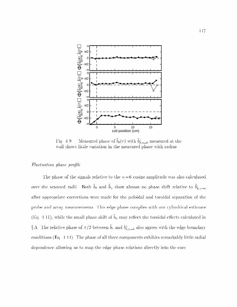
117

0 5 10 15coil position (cm)

π

π/2

0

-π/2

-ππ

π/2

0

-π/2

-ππ

π/2

0

-π/2

-π

Φb θ,

n= 6

( a)

,bθ( r

)(

)Φ

b θ,n=

6(a

),b

φ( r)

()

Φb θ,

n=6

( a)

,br( r

)(

)

Fig. 4.9.| Measured phase of ~b(r) with ~bc;n=6 measured at thewall shows little variation in the measured phase with radius.

Fluctuation phase prole

The phase of the signals relative to the n=6 cosine amplitude was also calculated

over the scanned radii. Both ~b and ~b show almost no phase shift relative to ~bc;n=6

after appropriate corrections were made for the poloidal and toroidal separation of the

probe and array measurements. This edge phase complies with our cylindrical estimate

(Eq. 4.11), while the small phase shift of ~b may re ect the toroidal eects calculated in

xA. The relative phase of =2 between ~br and bc;n=6 also agrees with the edge boundary

conditions (Eq. 4.14). The phase of all three components exhibits remarkably little radial

dependence allowing us to map the edge phase relations directly into the core.

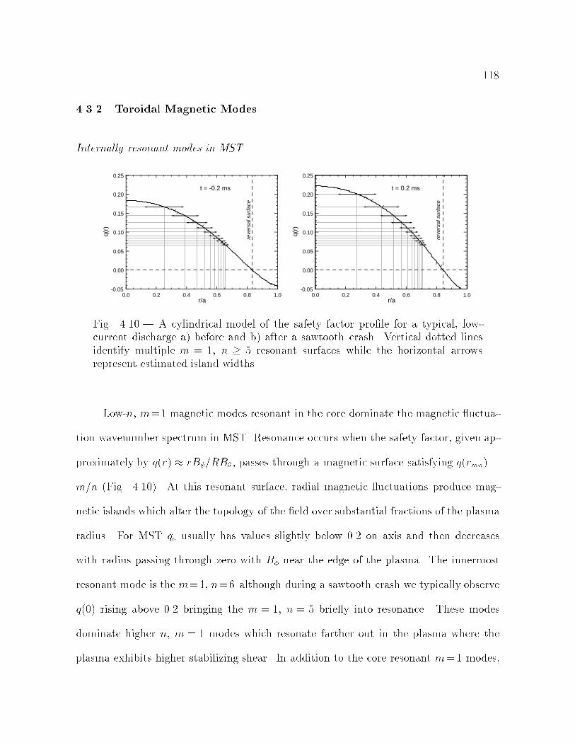
118

4.3.2 Toroidal Magnetic Modes

Internally resonant modes in MST

r/a

reve

rsal

sur

face

0.25

0.20

0.15

0.10

0.05

0.00

-0.050.0 0.2 0.4 0.6 0.8 1.0

q(r)

reve

rsal

sur

face

0.25

0.20

0.15

0.10

0.05

0.00

-0.050.0 0.2 0.4 0.6 0.8 1.0

q(r)

r/a

t = -0.2 ms t = 0.2 ms

Fig. 4.10.| A cylindrical model of the safety factor prole for a typical, low-current discharge a) before and b) after a sawtooth crash. Vertical dotted linesidentify multiple m = 1, n 5 resonant surfaces while the horizontal arrowsrepresent estimated island widths.

Low-n, m=1 magnetic modes resonant in the core dominate the magnetic uctua-

tion wavenumber spectrum in MST. Resonance occurs when the safety factor, given ap-

proximately by q(r) rB=RB , passes through a magnetic surface satisfying q(rmn) =

m=n (Fig. 4.10). At this resonant surface, radial magnetic uctuations produce mag-

netic islands which alter the topology of the eld over substantial fractions of the plasma

radius. For MST qo usually has values slightly below 0.2 on axis and then decreases

with radius passing through zero with B near the edge of the plasma. The innermost

resonant mode is the m=1, n=6 although during a sawtooth crash we typically observe

q(0) rising above 0.2 bringing the m = 1, n = 5 brie y into resonance. These modes

dominate higher n, m = 1 modes which resonate farther out in the plasma where the

plasma exhibits higher stabilizing shear. In addition to the core resonant m=1 modes,

119

theMSTplasm

acon

tainsm=0modes

resonantat

thereversal

surface.

These

modes

aredom

inated

bythem=0,n=1which

may

beresp

onsib

lefor

thethree-w

avecou

pling

ofadjacen

tm=1modes.

Usually

them=0modes

lockto

thelab

framethrou

ghout

thedisch

argemakingthem

dicultto

observe

with

thecoil

arrays.

How

ever,carefu

l

measu

rementswith

the~bcoil

arrayreveal

m=0,n=1am

plitu

des

comparab

leto

the

dom

inantm=1modes.

Thisisesp

eciallytru

eat

thecrash

where

enhanced

nonlinear

couplingbetw

eenthemodes

isobserv

edto

distrib

ute

pow

ertom=1modes

with

high

er

n.

Mode

dispersionover

thesaw

tooth

43210010

2030

frequency (kHz)

Pb

2(gauss /kHz)2

b)

300

200

1000-2-1

01

2tim

e (ms)

b2 (gauss )2 a)

56789≥10

toroidal mode number

Fig.

4.11.|a)

~b2;n (t)

ensem

bled

overasaw

toothwindow

.Thetotal

magn

etic uctu

ationpow

eristraced

outbythetop

curve.

Theligh

tanddark

bandsindicate

thedistrib

ution

ofpow

eram

ongthedom

inanttoroid

almodesas

indicated

bythe

key.b)Thepow

erspectra

ofthethemagn

etic uctu

ationswith

theindividual

modecon

tribution

sagain

denoted

bytheligh

tanddark

bands.

Atthesaw

toothcrash

thetotal

magn

etic uctu

ationpow

erpresen

tin

alltoroid

al

modes

increases

dram

aticallyfrom

atotal

~b2of30

gauss

2to

apeak

uctu

ationpow

erof

300gau

ss2(Fig.

4.11a).Follow

ingthecrash

the uctu

ationpow

erdrop

snearly

50%in

lessthan

50s,plateau

sfor

100s,andthen

decay

sover

thenext0.5

msto

itsbaselin

e

level.Thetwodecay

timescales

followingthecrash

appear

similarly

inall

ofthereson

ant

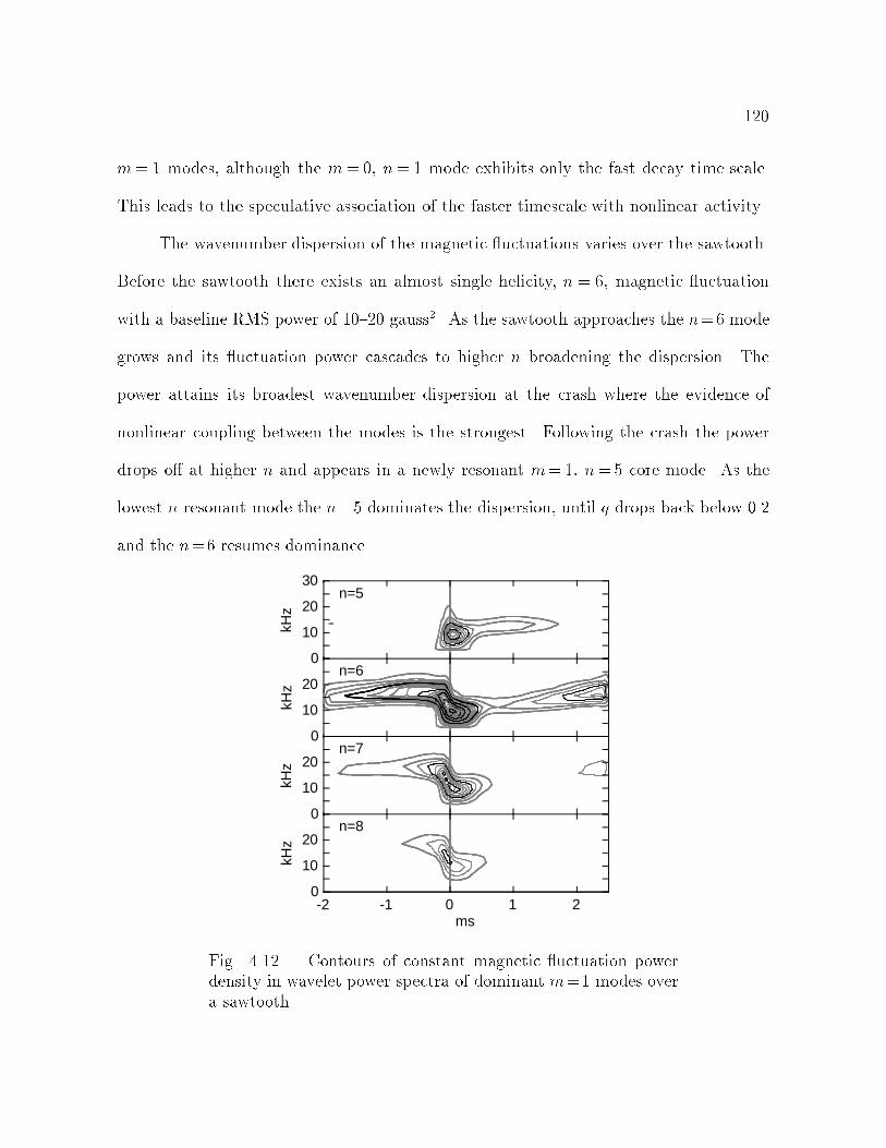
120

m= 1 modes, although the m= 0, n= 1 mode exhibits only the fast decay time scale.

This leads to the speculative association of the faster timescale with nonlinear activity.

The wavenumber dispersion of the magnetic uctuations varies over the sawtooth.

Before the sawtooth there exists an almost single helicity, n = 6, magnetic uctuation

with a baseline RMS power of 1020 gauss2. As the sawtooth approaches the n=6 mode

grows and its uctuation power cascades to higher n broadening the dispersion. The

power attains its broadest wavenumber dispersion at the crash where the evidence of

nonlinear coupling between the modes is the strongest. Following the crash the power

drops o at higher n and appears in a newly resonant m=1, n=5 core mode. As the

lowest n resonant mode the n=5 dominates the dispersion, until q drops back below 0.2

and the n=6 resumes dominance.

n=5

-2 -1 0 1 2ms

n=6

n=7

n=8

0

10

20

30

0

10

20

0

10

20

0

10

20

kHz

kHz

kHz

kHz

Fig. 4.12.| Contours of constant magnetic uctuation powerdensity in wavelet power spectra of dominant m=1 modes overa sawtooth.

121

The ensembled power spectrum (Fig. 4.11b) shows magnetic uctuation power

predominantly in the range of 820 kHz. The two peaks in the power spectrum may be

understood by referring to the wavelet power spectra (Fig. 4.12) for the four dominant

magnetic modes. This shows the power tracking the Doppler frequencies of the modes

in time accelerating away from the sawtooth and decelerating sharply at the sawtooth

crash. The fast pre-crash mode frequencies give rise to the peak near 17 kHz while the

slower postcrash frequencies produce the peak near 10 kHz. Note that the n=5 mode,

which only appears following the crash, exhibits power only about the lower frequency

peak.

4.3.3 \Average m" Calculation

n=1 n=6 n=11

n=2 n=7 n=12

n=3 n=8 n=13

n=4 n=9 n=14

n=5 n=10 n=15

MST 10 April, 1997, Shots #18-#422

1

02

1

02

1

02

1

02

1

0

-2 -1 0 1 2

time (ms)

-2 -1 0 1 2

time (ms)

-2 -1 0 1 2

time (ms)

mm

mm

m

Fig. 4.13.| m (Eq. 4.15) over the sawtooth for n=115.

While we believe the dominant toroidal mode numbers resolved by the toroidal

array to correspond to the core dominant m = 1 modes, full two-dimensional Fourier

122

decomposition is impossible with a single toroidal array. Instead, to obtain approximate

poloidal mode information we employed the coincident toroidal arrays of 32 ~b and 32 ~b

pickup coils to measure the full ~bn at the wall. Using Eq. 4.10 we may then dene,

m na

R

hb2;nihb2;ni

! 1

2

; (4.15)

where m, is commonly referred to as the \average m". Unfortunately, this terminology

is not wholly accurate as m generally does not equal a true power averaged m. That is

to say that in general,

hmi =P

mm~b2m;nP

m~b2m;n

6= m: (4.16)

However, without a full two dimensional array of coils we have no way of measuring hmi.

Furthermore, for toroidal modes dominated by a single poloidal mode number, m hmi.

Fig. 4.13 shows m for the fteen resolved toroidal modes ensembled over a low

current sawtooth cycle. For 5 n 10, m 1 corroborating our expectations that

these toroidal modes result from resonant m = 1 tearing modes. The slight dip in m

for these n for t 0 provides additional indication of enhanced m=0 nonlinear activity

at the sawtooth crash. For n= 1, m = 0 consistent with its resonance at the reversal

surface. For n > 10, m > 1 suggesting that these modes include m=2 coupling of lower

n internal modes. The highest m obtains for n = 13 possibly from three-wave m = 2

coupling of the dominant n=6 and n=7 modes.

4.3.4 Poloidal Phase Measurement

Diculties in properly determining the gains of the coils in the poloidal array,

prevents reliable Fourier decomposition of the m spectrum analogous that achieved for

the n spectrum with the toroidal array. Instead we have performed a study of the relative

123

π

π/20

-π/2-π-π-π/2

0π/2

πgeom

etric coil location

measured relative coil position

Fig.

4.14.|Themeasu

redrelativ

ephase

ofpoloid

alarray

coilsvs.their

poloid

alangle.

Deviation

sfrom

them=1line

arecon

sistentwith

outward

lyshifted

uxsurfaces.

uctu

ationphase

betw

eenindividualcoils

which

should

beindependentofthecoil

gains.

Therelative

phase

betw

eentwopoloid

allysep

aratedmeasu

rementsof

asin

glehelicity

magn

etic uctu

ationshould

begiv

enby,

( ~b

i ; ~bj )=m(

i j ):

(4.17)

For

m=1 uctu

ationsmeasu

redthisred

uces

tothepoloid

alsep

arationof

thecoils.

When

wecalcu

latetherelativ

ephase

ofthecoils

wendthat

torst

orderthe uctu

ation

exhibits

aclear

m=1stru

cture,

cyclin

gthrou

gh2

once

insin

glepoloid

altran

sit(Fig.

4.14).How

ever,thesim

plerelation

suggested

byEq.4.17

does

not

fully

describ

ethe

measu

redphase

dieren

ces.Acloser

tobtain

sfrom

theexpression

,

( ~b

i ; ~bj )=i

j

(sin

(i )

sin(

j )):(4.18)

Thisexpression

suggests

that

wecou

ldem

ploy

Eq.4.17

byrep

lacingwith

0given

by,

0=

sin

();(4.19)

124

where a simple t to the data yielded 0:34. This transformation of most likely

represents a conversion from machine geometry to ux surface geometry. In fact Eq.

4.19 roughly corresponds to the correction one would expect from outwardly shifted

ux surfaces. However, the size of the shift inferred from ( 14 cm) far exceeds

that predicted by toroidal models of the equilibrium. Nevertheless, we will employ Eq.

4.19 with the empirical to correct the poloidal position of subsequent uctuation

measurements.

4.3.5 Lundquist Number Scaling

ms-4 -2 0 2

Low S

Medium S

High S

3

2

1

0

2

1

0

2

1

0

%%

%

Fig. 4.15.| Ensembles of ~b=B(a) at each S.

We investigated the scaling of magnetic uctuations with Lundquist number using

the three large ensembles described in x 3.3.1. The ~b rms amplitude for each S is shown in

Fig. 4.15 as a percentage the edge poloidal eld. Neither the peak nor the baseline of the

125

normalized uctuations scales too dramatically remaining at 1% and 2% respectively

for all three ensembles. Rather, what scales with S is the eective duty cycle of the

uctuations. As noted in our discussion of the sawtooth period scaling (x 3.1.2) at higher

S settings the decay phase extends while the crash phase becomes more abrupt. Thus

the relative portion of the discharge during which the enhanced uctuation levels occur

decreases with S even though the actual uctuation levels at and away from the crash

remain unchanged.

106105S

b/B

0

10−3

10−2

b/B

0

10−3

10−2

a)

b)

S−0.01

S−0.03

S−0.01

S−0.08

S−0.13 S−0.08

Fig. 4.16.| a) max(~b=B) and b) hb=Biwin for the total rms uctuation amplitude (circle), the n = 7 amplitude (triangle)and the n = 10 amplitude (square).

This duty cycle eect may be seen in the two scalings shown in Fig. 4.16. The top

gure shows the absence of scaling of the peak uctuation amplitude with S,

max(~b) / S0:01: (4.20)

A similar result holds for scaling of the baseline uctuation level. However, by averaging

126

the uctuation level over the entire sawtooth cycle one recovers the eect of the decreasing

uctuation duty cycle and obtains a slight scaling of,

h~bi / S0:08: (4.21)

These scalings are somewhat weaker than those found by Stoneking et.al.(1997), for

which uctuations were averaged over xed time windows without regard to sawtooth

positions.

γavg (b)

6 8 10 12 14toroidal mode number

-0.20

-0.10

0.00

0.10

m=1 modes

Fig. 4.17.| The scaling exponent for avg(~b;n=B(a)). Thedashed line shows the scaling exponent for the total rms mag-netic uctuation amplitude (Eq. 4.21.

5 6 7 8 9toroidal mode number

before crash

after crash

%

40

10

20

30

0

10

20

30

0

%

Fig. 4.18.| ~b2n=~b2rms before and after the crash for high (circle),

medium (triangle), and low (square) S ensembles.

Fig. 4.16 also shows similar scaling for the n = 7 and n = 10 modes. These modes

127

become important later on in our discussion of the dynamo measurements. The scaling

exponents for the sawtooth averaged uctuations of other modes is shown in Fig. 4.17.

The scaling of the total uctuation amplitude scales like the n = 6 which dominates the

m = 1 uctuation energy with the other resonant modes scaling somewhat more strongly

as S0:12. Thus, we might expect the dispersion to become more peaked as we move to

higher S. This indeed occurs as illustrated in Fig. 4.18 before the sawtooth crash, where

we see a slightly higher fraction of the uctuation power contained in the n= 6 mode.

However, immediately following the crash the dispersion of the high S ensemble is much

broader indicating that the sawtooth crash distributes energy to high n more eectively

at higher currents.

References

Brotherton-Ratclie, D., C. G. Gimblett, and I. H. Hutchinson (1987). Plasma Phys.Controlled Fusion 29, 161.

Hutchinson, I. H., M. Malacarne, P. Noonan, and D. Brotherton-Ratclie (1984). Nucl.Fusion 24, 59.

La Haye, R. J., T. N. Carlstrom, R. R. Goforth, G. L. Jackson, M. J. Schaer, T. Tamano,and P. L. Taylor (1984). Phys. Fluids 27, 2567.

Stoneking, M. R., J. T. Chapman, D. J. Den Hartog, S. C. Prager, and J. S. Sar (1997).Experimental scaling of uctuations and connement with Lundquist number inthe RFP. Phys. Plasmas 5(4), 10041014.

128

5

Ion Velocity Fluctuations

In MHD theory the dynamics of the magnetic eld and the dynamics of the ion uid may

be viewed as two aspects of a single dynamic. Thus one expects the existence of large

scale perturbations in the magnetic eld to imply similar perturbations in the plasma

ow. Such uid velocity uctuations are observed in MHD computational simulations

and predicted in analytic treatments of the RFP. While magnetic perturbations in the

RFP have been thoroughly diagnosed through probe and edge measurements, the mea-

surement of uid uctuations has proven a greater diagnostic challenge, limited heretofore

to indirect observations at the edge.

In this chapter we report on new direct measurements of ion uid uctuations in

the core region of the MST. These measurements were conducted using the Ion Dynamics

Spectrometer, a passive spectroscopic diagnostic with a capacity to resolve fast, large-

scale uctuations. The capacity of the IDS for such measurements is discussed in detail

in Chapter 2 (esp x 2.5.2). The key results of these measurements are as follows:

Toroidal and poloidal ion velocity uctuations exist in MST with amplitudes of 1km/s and distributions in time and frequency resembling those observed for the

magnetic uctuations.

129

The velocity uctuations exhibit strong coherence with the magnetic uctuations

at the tearing mode frequencies prior to the sawtooth crash.

The phase between ~v and ~b is consistent with a non-zero dynamo product in the

MST core.

The relative phase between ~v and ~b is consistent with a superposition of two

eects: the advection of a parallel ow gradient past the IDS line of sight and

MHD uctuations producing an electric eld.

The radial prole of ~v(r) is narrower than that of ~b(r), consistent with MHD.

Radial velocity uctuations in MST are smaller than the measured ~v and ~v and

exhibit a very low coherence with the magnetic uctuations.

The normalized magnitude of ~v has weak scaling with S although its coherence

with the magnetics decreases dramatically at higher S.

This chapter employs the well diagnosed magnetic uctuations as a tool for investigating

the structure and dynamics of the velocity uctuations. While impacting the potential

for a nonlinear h~v ~bi dynamo electric eld in the MST, we postpone discussion of the

dynamo elds generated by the dynamo until next chapter.

We begin this chapter in x 5.1 by describing the distribution of velocity uctuation

power in frequency and time. We then investigate the coherence of these uctuations

with individual magnetic modes in x 5.2 and their phase relative to those modes in x 5.3.

In x 5.4 we describe the measurement of radial velocity uctuations. Finally, x 5.5 brie y

presents the scalings of ~v with S.

5.1 Velocity Fluctuation Power

The ensemble averaged uctuation power in frequency and time of chord averaged

velocity measurements, hP~v(f)i and h~v2(t)i, indicate the presence of 1 km/s ion veloc-

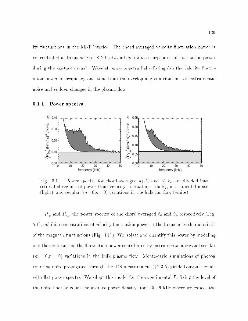
130

ity uctuations in the MST interior. The chord averaged velocity uctuation power is

concentrated at frequencies of 820 kHz and exhibits a sharp burst of uctuation power

during the sawtooth crash. Wavelet power spectra help distinguish the velocity uctu-

ation power in frequency and time from the overlapping contributions of instrumental

noise and sudden changes in the plasma ow.

5.1.1 Power spectra

0.00

0.05

0.10

0.15

0.20

0.25

0 10 20 30 40 50frequency (kHz)

Pv

φ(k

m/s

)2/kH

z

0.00

0.10

0.20

0.30

0.40

frequency (kHz)

Pvθ

(km

/s)

2/kH

z

0 10 20 30 40 50

a) b)

Fig. 5.1.| Power spectra for chord-averaged a) ~v and b) ~v are divided intoestimated regions of power from velocity uctuations (dark), instrumental noise(light), and secular (m=0,n=0) variations in the bulk ion ow (white).

P~v and P~v , the power spectra of the chord averaged ~v and ~v respectively (Fig.

5.1), exhibit concentrations of velocity uctuation power at the frequencies characteristic

of the magnetic uctuations (Fig. 4.11). We isolate and quantify this power by modeling

and then subtracting the uctuation power contributed by instrumental noise and secular

(m = 0,n = 0) variations in the bulk plasma ow. Monte-carlo simulations of photon

counting noise propagated through the IDS measurement (x 2.3.5) yielded output signals

with at power spectra. We adopt this model for the experimental P~v xing the level of

the noise oor to equal the average power density from 4549 kHz where we expect the

131

contributions from uctuations to be negligible. The uctuation power of the noise oor

determined in this fashion accounts for 52% and 60% of the total chord averaged ~v and

~v power, respectively.

We expect power from the secular evolution of the plasma ow to peak at low

frequency with a high frequency tail due to the rapid changes during the sawtooth crash.

Examining the spectra from 03 kHz, we observe that the power spectra minus the noise

oor, P~v(f) N~v, falls o roughly as e f . By extrapolating an exponential t to this

region out to higher frequencies we obtain a rough estimate for the high frequency tail of

the secular power contribution. For both measured spectra the power contained between

this curve and the noise oor accounts for approximately 20% of the total measured

uctuation power. Because most of this power is at low frequencies where we expect the

secular power to dominate, more accurate modeling of the high frequency tail should not

change this number by more than a few percent.

Having accounted for noise and secular power in the spectra we are left with a region

of velocity uctuation power comprising 2030% of the original measured power in the

IDS signal. The uctuations are particularly well resolved in the ~v power spectrum,

which plateaus from 1020 kHz where we expect the majority of the velocity uctuation

power to be located. To estimate the true magnitude of the velocity uctuation we must

correct for the attenuation of the velocity uctuation amplitude by the chord average. For

the toroidal chord, extremely simple models of m=1, n=6 ~v(r) uctuation proles upon

convolution with the toroidal chord instrument function retain between 12% and 18%

of their amplitude. A ~v(r) with an optimal prole relative to the instrument function

retains only 20% of its amplitude. For the m = 1, n = 7 mode, typical prole models

retain 10% to 15% of their amplitudes with the optimal mode retaining only 16%. The

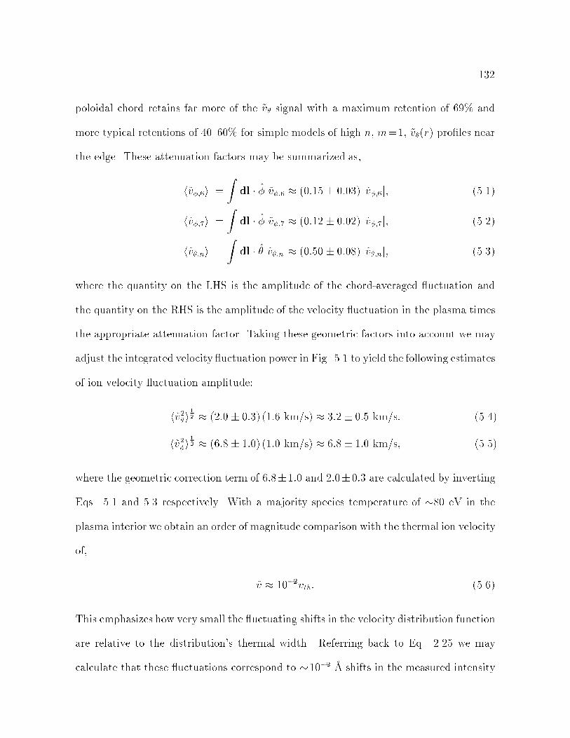
132

poloidal chord retains far more of the ~v signal with a maximum retention of 69% and

more typical retentions of 4060% for simple models of high n, m=1, ~v(r) proles near

the edge. These attenuation factors may be summarized as,

jh~v;6ij =Zdl ~v;6 (0:15 0:03) j~v;6j; (5.1)

jh~v;7ij =Zdl ~v;7 (0:12 0:02) j~v;7j; (5.2)

jh~v;nij =Zdl ~v;n (0:50 0:08) j~v;nj; (5.3)

where the quantity on the LHS is the amplitude of the chord-averaged uctuation and

the quantity on the RHS is the amplitude of the velocity uctuation in the plasma times

the appropriate attenuation factor. Taking these geometric factors into account we may

adjust the integrated velocity uctuation power in Fig. 5.1 to yield the following estimates

of ion velocity uctuation amplitude:

h~v2i1

2 (2:0 0:3) (1:6 km/s) 3:2 0:5 km/s: (5.4)

h~v2i1

2 (6:8 1:0) (1:0 km/s) 6:8 1:0 km/s; (5.5)

where the geometric correction term of 6:81:0 and 2:00:3 are calculated by inverting

Eqs. 5.1 and 5.3 respectively. With a majority species temperature of 80 eV in the

plasma interior we obtain an order of magnitude comparison with the thermal ion velocity

of,

~v 102vth: (5.6)

This emphasizes how very small the uctuating shifts in the velocity distribution function

are relative to the distribution's thermal width. Referring back to Eq. 2.25 we may

calculate that these uctuations correspond to 102 A shifts in the measured intensity

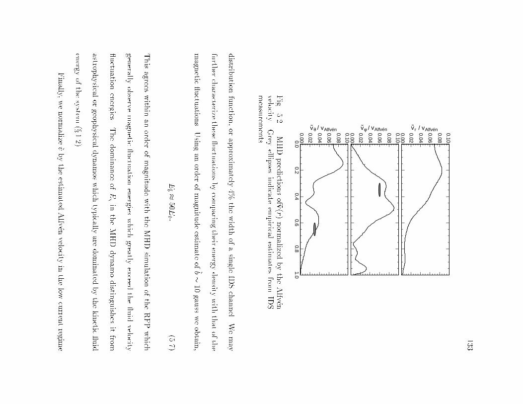
133

0.00.2

0.40.6

0.81.0

0.00

0.02

0.04

0.06

0.08

0.10

v r / vAlfvénvφ / vAlfvénvθ / vAlfvén 0.00

0.02

0.04

0.06

0.08

0.100.00

0.02

0.04

0.06

0.08

0.10

Fig.

5.2.|MHD

pred

ictionsof~v

(r)norm

alizedbytheAlfven

velocity.Grey

ellipses

indicate

empirical

estimates

fromIDS

measu

rements.

distrib

ution

function

,or

approx

imately

4%thewidth

ofasin

gleIDSchannel.

Wemay

furth

ercharacterize

these

uctu

ationsbycom

parin

gtheir

energy

density

with

that

ofthe

magn

etic uctu

ations.Usin

gan

order

ofmagn

itudeestim

ateof~b

10gau

ssweobtain

,

E~b

50E~v :

(5.7)

Thisagrees

with

inan

order

ofmagn

itudewith

theMHDsim

ulation

oftheRFPwhich

generally

observe

magn

etic uctu

ationenergies

which

greatlyexceed

the uid

velocity

uctu

ationenergies.

Thedom

inance

ofE~bin

theMHD

dynam

odistin

guish

esitfrom

astrophysical

orgeop

hysical

dynam

oswhich

typically

aredom

inated

bythekinetic

uid

energy

ofthesystem

(x1.2).

Finally,

wenorm

alize~vbytheestim

atedAlfven

velocityin

thelow

curren

tregim

e

134

obtaining,

h~v2i1

2 =vAlfven 0:03; (5.8)

h~v2i1

2 =vAlfven 0:06; (5.9)

where we have employed vAlfven of 110 km/s (Table 3.1). Overplotting these estimates

onto the ~v(r) proles modeled with the MHD code (Fig. 5.2) we see remarkable agree-

ment with the measurements, nearly coinciding with the modeled ~v(r) and ~v(r) curves.

While the detailed agreement of the model and measurements may be fortuitous, clearly

the velocity uctuation measured in the core possess a magnitude consistent with the

predictions of MHD.

5.1.2 Power distribution over a sawtooth

25

20

15

10

5

0

time (ms)-1 0 1 2

vθ2

(km

/s)2

a) 15

10

5

0

time (ms)-1 0 1 2

vφ2

(km

/s)2

b)

Fig. 5.3.| Average a) poloidal and b) toroidal velocity uctuation power (dark)over a sawtooth crash. The noise- oor (light) is distributed proportionately toh2i (Eq. 2.27).

The velocity uctuation power rises sharply at the sawtooth crash reaching peak

level of several (km/s)2 (Fig. 5.3). The noise power estimated from the power spectrum

may be distributed in time proportionately to the 2 according to the error propagation

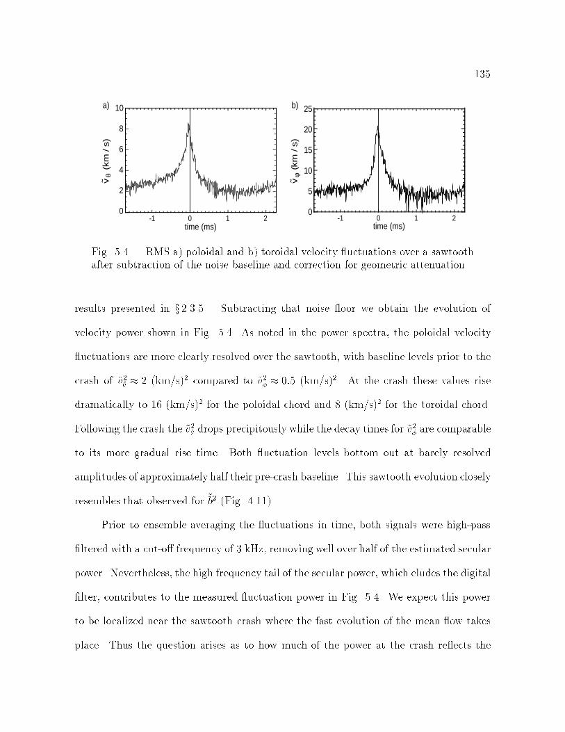
135

time (ms)-1 0 1 2

vθ

(km

/s)

a)

time (ms)-1 0 1 2

vφ

(km

/s)

b)

0

10

2

4

6

8

0

5

10

15

20

25

Fig. 5.4.| RMS a) poloidal and b) toroidal velocity uctuations over a sawtoothafter subtraction of the noise baseline and correction for geometric attenuation.

results presented in x 2.3.5 . Subtracting that noise oor we obtain the evolution of

velocity power shown in Fig. 5.4. As noted in the power spectra, the poloidal velocity

uctuations are more clearly resolved over the sawtooth, with baseline levels prior to the

crash of ~v2 2 (km/s)2 compared to ~v2 0:5 (km/s)2. At the crash these values rise

dramatically to 16 (km/s)2 for the poloidal chord and 8 (km/s)2 for the toroidal chord.

Following the crash the ~v2 drops precipitously while the decay times for ~v2 are comparable

to its more gradual rise time. Both uctuation levels bottom out at barely resolved

amplitudes of approximately half their pre-crash baseline. This sawtooth evolution closely

resembles that observed for ~b2 (Fig. 4.11).

Prior to ensemble averaging the uctuations in time, both signals were high-pass

ltered with a cut-o frequency of 3 kHz, removing well over half of the estimated secular

power. Nevertheless, the high frequency tail of the secular power, which eludes the digital

lter, contributes to the measured uctuation power in Fig. 5.4. We expect this power

to be localized near the sawtooth crash where the fast evolution of the mean ow takes

place. Thus the question arises as to how much of the power at the crash re ects the

136

0

10

20

30

40

50

-2 -1 0 1 2ms

kHz

0

10

20

30

40

50

-2 -1 0 1 2ms

kHz

b)

a)

Fig. 5.5.| Contours of constant power density in the averaged a) ~vand b) ~v wavelet power spectra. Two peaks appear in the bottomcontour at 5 and 10 kHz near the sawtooth crash.

137

growth of velocity uctuations and how much is due to the fast secular changes. The

wavelet power spectra of the uctuations provides a partial answer to this question (Fig.

5.5). Examining the distribution for ~v at the crash, one observes two distinct peaks

in the power distribution. The \peak" at 5 kHz is the high frequency remnant of the

secular power peak at 0 kHz removed by the high-pass lter. The apparent broad time

duration of this residual secular power about the crash re ects the poor time resolution

of the wavelet analysis at low frequencies (Eq. 3.19). A second distinct peak occurs at 10

kHz with the power dropping slowly out to 20 kHz. This peak provides clear evidence of

velocity uctuations concentrated near the crash. Integrating the power beneath the two

peaks we nd that the power from 38 kHz is roughly half of that from 820 kHz. This

integration gives an approximate correction of two-thirds to the peak velocity uctuation

near the crash. In the ~v distribution the two peaks merge into a ridge which extends

from the secular to the uctuation frequencies.

5.2 Coherence of Velocity and Magnetic Fluctuations

0.00

0.10

0.20

0.30

0.40

frequency (kHz)0 10 20 30 40 50

a) b)

0.00

0.10

0.20

0.30

0.40

-2 -1 0 1 2time (ms)

γ v φb

θ( f)

γ v φb

θ( t)

Fig. 5.6.| The measured coherence of the toroidal ion velocity uctuations withan edge magnetic coil in a) frequency (Eq. 3.14) and b) time (Eq. 3.11). Thedashed line represents the coherence baseline.

138

Above we noted similarities in the frequency distribution of magnetic uctuation

power, P~b (Fig. 4.11b), and velocity uctuation power, P~v (Fig. 5.1) and common

features in the time evolution of ~b2 (Fig. 4.11a) and ~v2 (Fig. 5.3). These observations

strongly suggest that the uctuations in magnetic eld and ion ow are dynamically

coupled. We conrm this through the measurement of signicant coherence between the

two quantities in time and frequency. Fig. 5.6 illustrates such coherence between ~v and

the ~b from a single edge coil. In frequency we see a coherence level of 0.2 or higher

from 515 kHz while in time the coherence peaks immediately prior to the sawtooth.

Subsequent paragraphs explore these dynamics in detail characterizing the coherence of

~b with ~v and ~v over the three dimensional domain of time, frequency and wavenumber.

We conclude that the distribution of coherence in time and frequency largely re ects the

distribution of ~b2(f; t) and ~v2(f; t). In wavenumber the incidence of coherence does not

match the measured dispersion of ~b;n re ecting instead the changing sensitivity of the

IDS chord to the dierent wavenumbers. Lastly, a sharp rise in coherence prior to the

sawtooth crash suggests enhanced uctuation coupling while a dramatic drop at the crash

suggests a scrambling of the uctuation phase.

5.2.1 Coherence with Individual Modes | Description

The velocity uctuations measured by the IDS may be expressed as the weighted

sum of uctuations with various wavenumbers,

~v =Xn

Cn~vn; (5.10)

where Cn depends on the convolution of the radial mode structure with the IDS instru-

ment function and the CV emission prole. If we assume that all activity in the plasma

at the resonant wavenumbers in the plasma occurs with a coherent phase relation to the

139

magnetic perturbations we may employ our knowledge of the magnetic perturbations

to extract mode information from the velocity uctuations. The rotation of the low n

magnetic modes converts their spatial structure in the plasma frame into a temporal

variation in the lab frame. This allows the use of ~b;n as a set of time dependent basis

functions for the spatial Fourier analysis of ~v,

h~v~b;ni =Xn0

Cn0h~vn0~b;ni Cnh~vn~b;ni: (5.11)

By normalizing this product by the velocity and magnetic uctuation power (i.e. calcu-

lating the coherence), we hope to extract information about both Cn and vn. Below we

present the full wavelet coherence spectra of ~b;n with ~v and ~v for n=615. This allows

the simultaneous description of the coherence dynamics over wavenumber, frequency, and

time. The following paragraphs will introduce these spectra by describing the important

features which are observed. Interpretation of the spectra in terms of underlying physical

and instrumental phenomena will be provided in the following subsection (x 5.2.2).

Coherence of poloidal velocity uctuations

Subdominant magnetic perturbations with toroidal mode numbers of eight and

above exhibit high coherence levels with ~v. The coherence levels increase steadily over

the low n modes from a peak value of just 20% for the dominant n=6 mode to a peak

value of nearly 50% for relatively small n=9 mode. At higher n the coherence drops o

slowly maintaining reasonable levels out to the tiny n=14 mode, which achieves a higher

peak coherence than that achieved by the enormous n = 6 mode. The distribution of

coherence in frequency and time re ects that observed in the single coil coherence levels

of Fig. 5.6. The resolved modes exhibit robust coherence over the full sawtooth cycle

tracking the accelerations and decelerations of the dominant ~b frequencies in time. Just

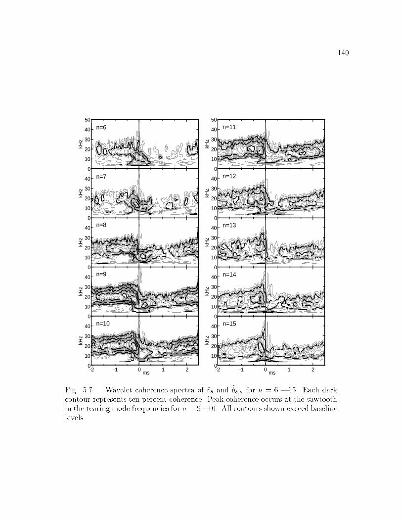
140

-2 -1 0 1 2ms

n=11

n=12

n=13

n=14

n=15n=10

n=6

n=7

n=8

n=9

-2 -1 0 1 2ms

40

30

20

10

0

40

30

20

10

0

40

30

20

10

0

40

30

20

10

0

40

30

20

10

0

50

kHz

kHz

kHz

kHz

kHz

40

30

20

10

0

40

30

20

10

0

40

30

20

10

0

40

30

20

10

0

40

30

20

10

0

50

kHz

kHz

kHz

kHz

kHz

Fig. 5.7.| Wavelet coherence spectra of ~v and ~b;n for n = 6 15. Each darkcontour represents ten percent coherence. Peak coherence occurs at the sawtoothin the tearing mode frequencies for n = 910. All contours shown exceed baselinelevels.

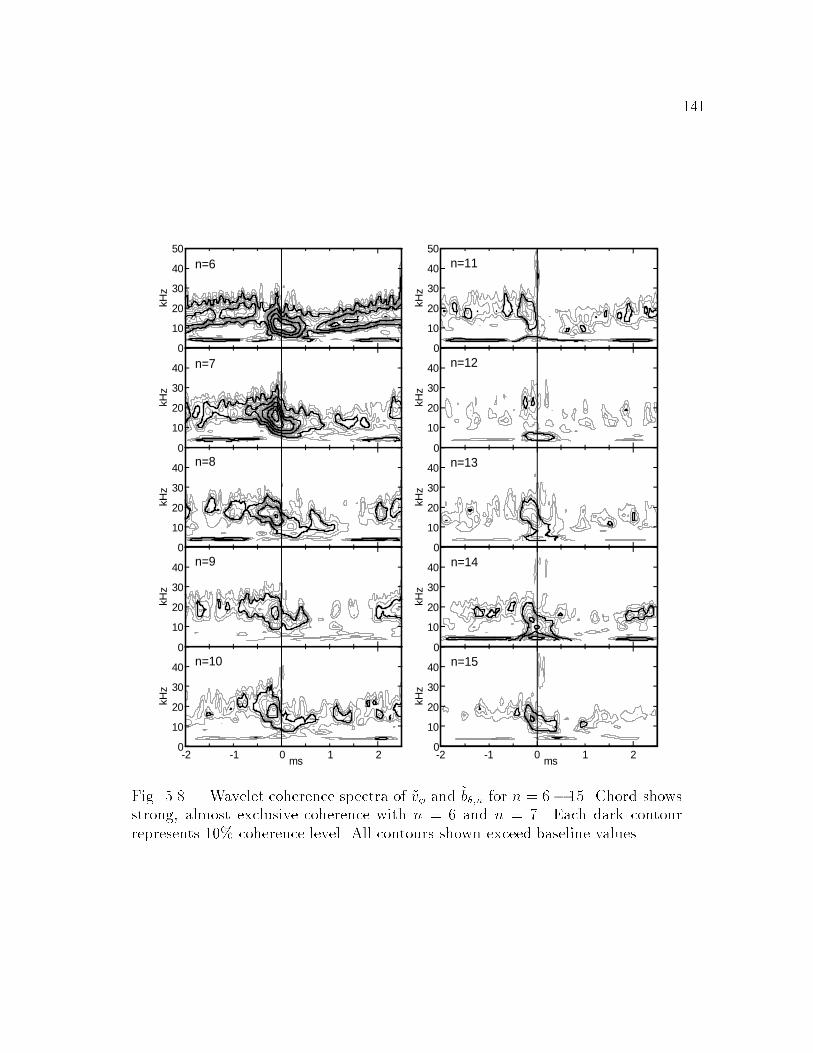
141

-2 -1 0 1 2ms

n=11

n=12

n=13

n=14

n=15n=10

n=6

n=7

n=8

n=9

-2 -1 0 1 2ms

40

30

20

10

0

40

30

20

10

0

40

30

20

10

0

40

30

20

10

0

40

30

20

10

0

50

kHz

kHz

kHz

kHz

kHz

40

30

20

10

0

40

30

20

10

0

40

30

20

10

0

40

30

20

10

0

40

30

20

10

0

50

kHz

kHz

kHz

kHz

kHz

Fig. 5.8.| Wavelet coherence spectra of ~v and ~b;n for n = 6 15. Chord showsstrong, almost exclusive coherence with n = 6 and n = 7. Each dark contourrepresents 10% coherence level. All contours shown exceed baseline values.

142

prior to the sawtooth crash ~v~b peaks along with the ~v and ~b uctuation levels before

it drops precipitously at the crash to roughly half its peak value. Modes with n=6 9

exhibit a second coherence peak 0.2 ms after the crash, whereas the higher n modes

exhibit only a slow rebuilding back to their pre-crash levels over 12 ms.

Coherence of toroidal velocity uctuations

The large n=6 and n=7 modes dominate the wavenumber dispersion of ~v~b;n(f; t)

(Fig. 5.8) in sharp contrast to the dispersion observed for ~v~b;n. The toroidal velocity

coherence falls o dramatically for n 8 reaching near baseline values over most of the

coherence spectrum for n > 10. Of the two peak modes the highest coherence appears

just prior to the crash for the n = 7 where ~v~b;7(f; t) 0:6.1 In time ~v~b;n behaves

similarly to ~v~b;n, peaking just prior to the crash where it drops dramatically, rebounding

a fraction of a ms later in a second peak for n 9. However, unlike the poloidal chord

only the n=6 exhibits robust coherence over the full sawtooth cycle.

5.2.2 Coherence with Individual Modes | Interpretation

Figs. 5.75.8 depict coherence levels for each chord with complex, and often sur-

prising, variations in frequency, time, and wavenumber. To structure our interpretation

of these dynamics we enumerate three distinct factors which together determine ~v~b:

1. The presence of uctuations with amplitudes comparable to or greater than the

instrumental noise levels.

2. The actual coherence of the ion velocity uctuations with the magnetic uctuations

1This measurement holds the current record for the highest coherence ever measured between achord averaged IDS ~v measurement and a second independent uctuation. The ability to achieve sucha high coherence a signal as noisy as the IDS derives from the combination of large ensemble analysis,spatial Fourier isolation of the dominant ~b modes, and resolution, via wavelet analysis, of coherence overfrequency and time.

143

in the MST plasma.

3. The sensitivity of the IDS chord to the wavenumber and radial structure of each

mode.

Below we attempt to associate phenomena observed in ~v~b;n(f; t) and ~v~b;n(f; t) with

the appropriate factors. First, we examine when the measured coherence re ects the

presence of uctuations and when it re ects the actual coherence of those uctuations.

Then we discuss the interaction of dierent wavenumbers with the poloidal and toroidal

IDS chords, in an attempt to explain the unusual wavenumber dispersion of each view.

Measured coherence of noisy signals

In x 3.2.3 we dened the coherence of two uctuating signals as the percentage of

the signals' power which exhibits a non-random relative phase. For noiseless uctuation

measurements, this holds true as the amplitudes of the uctuations divide out of the

measured coherence perfectly. However with the introduction of instrumental noise a

portion of the uctuation power from one or both signals will exhibit a random phase,

regardless of the actual coherence of the uctuations in the plasma. This introduces a

dependence of the measured coherence on the relative amplitude of the uctuations and

the instrumental noise. For the IDS measurement with 50% or greater noise levels this

eect may be dramatic. We quantify this dependence by rewriting the expression for

coherence taking noise into account,

2~v~b=

jh~v~bij2h~v2 +N2

~v ih~b2 +N2~bi ; (5.12)

where N~v and N~b are the velocity and magnetic noise levels respectively. When ~v2 N2~v

and ~b2 N2~bthe dependence of ~v~b on the amplitudes of the uctuations diminishes,

144

and more accurately re ects the true coherence of the signals. When the converse is

true for either signal the measured coherence re ects both the physical coherence of the

uctuations and the signal to noise ratio of the measurement. This is the limit generally

appropriate to the IDS. The dependence of coherence on the presence of substantial

uctuation amplitude explains the basic and expected features in Fig. 5.75.8, including

the distribution of coherence in frequency and the gross evolution of the coherence over

the sawtooth.

The dramatic rise and fall of the coherence near the sawtooth cannot be explained

by signal to noise dynamics in Eq. 5.12. Prior to the crash the rising amplitude of the

velocity uctuations in the tearing mode frequencies grow to satisfy ~v2 N2~v . and rough

calculations indicate signal-to-noise eects on the coherence saturate 0.5 ms before

the crash. Nevertheless the measured coherence continues to rise indicating that the

uctuations actually become more coherent prior to the crash. More dramatically, at the

crash the drop in coherence precedes and exceeds the decay of the uctuation amplitudes

suggesting a phase scrambling of the uctuations by the sawtooth. For the dominant

modes this randomization is brief and the coherence bounces back following the crash,

falling o more gradually after that along with the diminishing uctuation amplitudes.

Here I propose a scenario which is largely consistent with the observations, that

may explain the sudden rise and fall of the measured coherence about the crash. Prior

to the crash power concentrates in the dominant modes which lock together forming a

structure often referred to as \slinky". The eect of this locking is to make Eq. 5.11

break down as h~vn0~bn;i becomes nonzero for n0 6= n. Hence, uctuation wavenumbers

other than the one being correlated with ~b;n develop a nonrandom phase relationship with

the correlated mode and contribute to the measured coherence. In short, phase locking

145

of the modes induces leakage of the coherence with indiviudal modes to the measured

coherence of adjacent modes producing a net rise in the overall measured coherence. At

the crash two things happen. First, nonlinear coupling distributes power to higher n

modes. Second,the modes decouple with their relative phase reset by the crash. This

combination pulls power out of the low n dominant modes and then cuts o the leakage

of those high n modes back to low n. This produces a coherence crash for the dominant

resolved modes. Shortly after the crash, however, the low nmodes regain their dominance

of the power dispersion producing a return of much of their measured coherence. The

phases remain unlocked for several ms leaving the higher n modes with little power and

no coherence leakage from the high n modes. Hence, their coherence remains low until

the onset of phase locking at the next crash

Coherence vs. n re ects resolution of IDS chord

0.30

0.25

0.20

0.15

0.10

0.05

0.000 5 10 15

toroidal mode number

aver

age

cohe

renc

e

Fig. 5.9.| Coherence of ~v (solid) and ~v (grey) with ~b;n av-eraged in frequency from 7 to 20 kHz, and in time over the fullsawtooth cycle.

A prominent exception to the variation of the measured coherence with the uc-

tuation amplitude may be found in the wavenumber dependence of ~v~b;n and ~v~b;n.

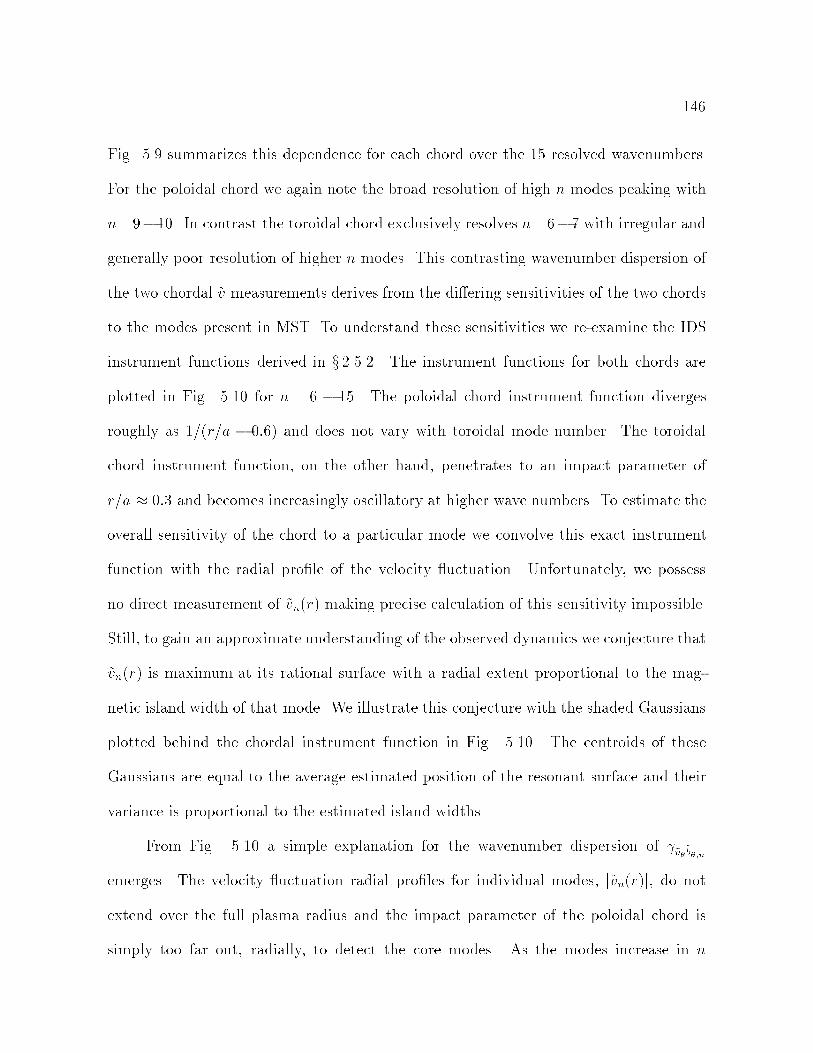
146

Fig. 5.9 summarizes this dependence for each chord over the 15 resolved wavenumbers.

For the poloidal chord we again note the broad resolution of high n modes peaking with

n=910. In contrast the toroidal chord exclusively resolves n=67 with irregular and

generally poor resolution of higher n modes. This contrasting wavenumber dispersion of

the two chordal ~v measurements derives from the diering sensitivities of the two chords

to the modes present in MST. To understand these sensitivities we re-examine the IDS

instrument functions derived in x 2.5.2. The instrument functions for both chords are

plotted in Fig. 5.10 for n = 6 15. The poloidal chord instrument function diverges

roughly as 1=(r=a 0:6) and does not vary with toroidal mode number. The toroidal

chord instrument function, on the other hand, penetrates to an impact parameter of

r=a 0:3 and becomes increasingly oscillatory at higher wave numbers. To estimate the

overall sensitivity of the chord to a particular mode we convolve this exact instrument

function with the radial prole of the velocity uctuation. Unfortunately, we possess

no direct measurement of ~vn(r) making precise calculation of this sensitivity impossible.

Still, to gain an approximate understanding of the observed dynamics we conjecture that

~vn(r) is maximum at its rational surface with a radial extent proportional to the mag-

netic island width of that mode. We illustrate this conjecture with the shaded Gaussians

plotted behind the chordal instrument function in Fig. 5.10. The centroids of these

Gaussians are equal to the average estimated position of the resonant surface and their

variance is proportional to the estimated island widths.

From Fig. 5.10 a simple explanation for the wavenumber dispersion of ~v~b;n

emerges. The velocity uctuation radial proles for individual modes, j~vn(r)j, do not

extend over the full plasma radius and the impact parameter of the poloidal chord is

simply too far out, radially, to detect the core modes. As the modes increase in n

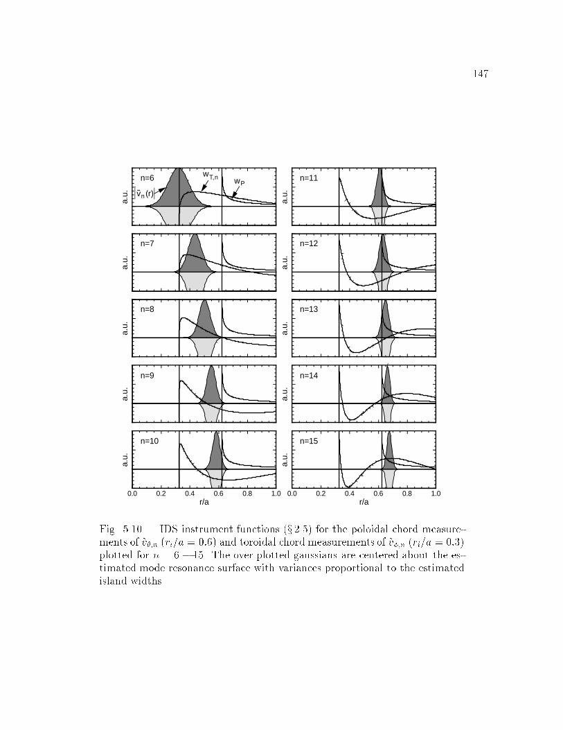
147

0.0 0.2 0.4 0.6 0.8 1.0r/a

0.0 0.2 0.4 0.6 0.8 1.0r/a

n=6

n=7

n=8

n=9

n=10

n=11

n=12

n=13

n=14

n=15

vn (r)

wPwT,n

a.u.

a.u.

a.u.

a.u.

a.u.

a.u.

a.u.

a.u.

a.u.

a.u.

Fig. 5.10.| IDS instrument functions (x 2.5) for the poloidal chord measure-ments of ~v;n (ri=a = 0:6) and toroidal chord measurements of ~v;n (ri=a = 0:3)plotted for n = 6 15. The over plotted gaussians are centered about the es-timated mode resonance surface with variances proportional to the estimatedisland widths.

148

their resonant surfaces move outward and more of their uctuation power falls along the

poloidal line of sight. The peak measured coherence at n=9 suggests that the resonance

surface for the modes may lie farther out in radius than the positions estimated by the

cylindrical equilibrium model such as might be expected by an outward Shafranov shift

of the plasma column. The poloidal chord coherence clearly implies that the velocity

uctuations for each mode extend over a fraction of the machine radius in contrast to

the magnetic perturbations which extend coherently from the plasma interior to the wall.

The high coherence of the n=12 mode compared to the n=6 mode is particularly strik-

ing evidence of this. This result invites measurements to be made at additional impact

parameters to produce mode resolved reconstructions of ~v;n(r).

The complex wavenumber dependence of ~v~b;n derives from the convolution of

uctuation power which moves out in radius with n and an instrument function which

becomes increasingly oscillatory with increased n. While the impact parameter of the

toroidal chord falls outside the estimated position of the n=6 rational surface, much of

the uctuation power in this large mode falls within view of the chord accounting for a

large measured coherence. For n=7 the bell of the instrument function moves slightly

inward and the rational surface moves slightly outward resulting in the fortuitous overlay

of uctuation power with instrumental resolution. The fact that the maximum coherence

peaks is attained for this mode which is roughly half the size of the n = 6, indicates

that ~v;n(r) like ~v;n(r) possesses limited radial extent. As we move to n = 8 9 the

uctuation power coincides with the null in the instrument function yielding a minimum

in the measured coherence. With increasing n the measured coherence moves up and

down as the velocity uctuation proles coincide with the hills, valleys, and nulls of

the toroidal instrument function. This intermittent coherence at high n again suggests

149

sharply dened velocity uctuation proles for each mode. If the power from these high

n modes were broadly distributed in radius their short wavelengths would be averaged

over by the toroidal chord. However, localized, high-n uctuation power may act like a

delta function, picking out the value of the IDS instrument function at the radius of its

peak activity. This is one possible explanation for a baseline coherence level achieved for

the tiny n=12 mode followed by a jump in coherence for the even tinier n=14 mode.

The latter reaches peak coherence levels exceeded only by the dominant n=6 and n=7

modes. Localized uctuation amplitudes might also produce time dynamics in ~v~b as

individual high n modes move in and out of view. Unfortunately, our limited knowledge

of the precise form or location of ~vn(r) prevents the identication of such eects.

5.3 Fluctuation Phase

In this section we examine the phase between the chord averaged velocity uctu-

ations ~v and ~v and the uctuating magnetic eld. We begin with the frequency and

time behavior of the measured phase for h~v~b;n=9i and h~v~b;n=7i. Next we derive a map

from the measured h~v~bi phase, (~v;~b), to an average local uctuation phase, hv bi.

Finally, we present and interpret the local phase of ~v and ~v relative to the magnetics.

5.3.1 Measured chord-averaged phase versus time and frequency

Fig. 5.11a shows the measured phase and coherence between the chord-averaged

poloidal ion velocity uctuation and the cosine amplitude of the n = 9 toroidal mode.

Prior to the sawtooth as the coherence rises near 0.3, the measured phase becomes more

cleanly resolved, however its mean value does not appear to change. Following the crash

the mean phase does change, rising nearly 30o and becomes less well resolved as the

150

-2 -1 0 1 2-π

-π/2

0

π/2

π

time (ms)

0.0

0.2

0.4

0.6

0.8

1.0a)Φ

(vθ, b

θ,9)

c

γ(v

θ ,bθ,9

)c

-2 -1 0 1 2-π

-π/2

0

π/2

π

time (ms)

0.0

0.2

0.4

0.6

0.8

1.0b)

cΦ

(vφ, b

θ,7)

),

γ(v

φb

θ,7

c

Fig. 5.11.| Grey line denotes the measured phase of a) h~vb;n=9i and b) h~vb;n=7iover a sawtooth. The darkly shaded region at the bottom of both plots representsthe measured coherence while the lightly shaded region represents the coherencebaseline.

coherence drops near baseline levels. The measured phase of h~vb;n=7i (Fig. 5.11b)

exhibits similar time dynamics, although away from the sawtooth the coherence is lower

and the phase, therefore, is more poorly resolved.

A partial explanation for the dynamics of the phase versus timemay be found in the

complementary behavior of the phase versus frequency, (Fig. 5.12). The relative phase

of both products decreases as frequency increases. Thus prior to the crash the rapidly

rotating high frequency uctuations sample the lower phase region of the spectra, while

after the crash the decelerated modes sample the high-phase, low-frequency portion of the

spectra. The negative slope of the phase with frequency is consistent with a uniform time

delay of 7.5 s between ~v and ~b;n=9, and a time delay of 9.3 s between ~v and ~b;n=7,

where the magnetic uctuations lag the velocity uctuations in both cases. A check of the

analog processing for both ~v and ~b measurements found the systems to be synchronous

to within one s following the correction (implemented in the fit.pro code) for the 3.64

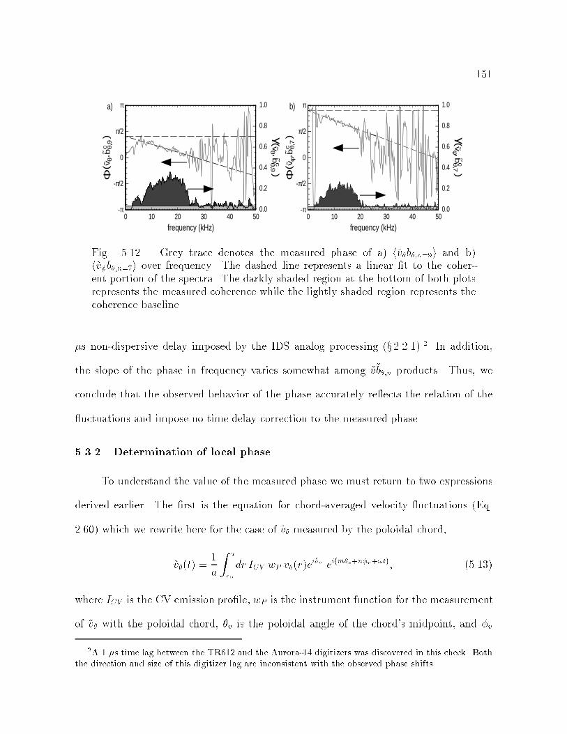
151

-π

-π/2

0

π/2

π

0.0

0.2

0.4

0.6

0.8

1.0a)

0 10 20 30 40 50

frequency (kHz)

Φ( v

θ, b

θ,9)

c

γ(v

θ ,bθ,9

)c

-π

-π/2

0

π/2

π

0.0

0.2

0.4

0.6

0.8

1.0b)

Φ( v

φ, b

θ,7)

c

)γ(v

φ ,bθ,7

c

0 10 20 30 40 50

frequency (kHz)

Fig. 5.12.| Grey trace denotes the measured phase of a) h~vb;n=9i and b)h~vb;n=7i over frequency. The dashed line represents a linear t to the coher-ent portion of the spectra. The darkly shaded region at the bottom of both plotsrepresents the measured coherence while the lightly shaded region represents thecoherence baseline.

s non-dispersive delay imposed by the IDS analog processing (x 2.2.1).2 In addition,

the slope of the phase in frequency varies somewhat among ~v~b;n products. Thus, we

conclude that the observed behavior of the phase accurately re ects the relation of the

uctuations and impose no time delay correction to the measured phase.

5.3.2 Determination of local phase

To understand the value of the measured phase we must return to two expressions

derived earlier. The rst is the equation for chord-averaged velocity uctuations (Eq.

2.60) which we rewrite here for the case of ~v measured by the poloidal chord,

~v(t) =1

a

Z a

ro

dr ICV wP v(r)eiv ei(mv+nv+!t); (5.13)

where ICV is the CV emission prole, wP is the instrument function for the measurement

of ~v with the poloidal chord, v is the poloidal angle of the chord's midpoint, and v

2A 1 s time lag between the TR612 and the Aurora-14 digitizers was discovered in this check. Boththe direction and size of this digitizer lag are inconsistent with the observed phase shifts.

152

0 5 10 150

5π

10π

15π

toroidal mode number

Φ( v

θ,b θ

,n)

θv θb-( ) δv δb-( )+φvn +

6π8π 8π 10

π 12π

12π 14

π14

π 16π

4πFig. 5.13.| Grey circles denote the measured phase ofh~vb;ni for n = 5 15. Adding an integer multiple of2 the points fall along a line with a slope equal to thetoroidal angle of the ~v measurement and an interceptwhich yields the local relative phase of ~v and ~b.

is the toroidal location of the chord. This expression expands the measured ~v as a

weighted integral of v(r) and its complex phase angle, eiv. Outside the integral, the

time dependent exponential, ei!t, is multiplied by a reference phase angle determined by

the position of the chord and the helicity of the mode. The second expression we need

(Eq. 4.1) denes ~b;n as,

~b;n(t) = b;nei(mb+!t+b); (5.14)

where b is the poloidal angle of the toroidal array coils. Using these two expressions we

may evaluate the ensemble averaged product of ~v and ~b;n , obtaining,

h~v~b;ni = 1

a

Z a

ro

dr ICV wP hv(r) b;n ei(vb)i ei(m(vb)+nv): (5.15)

By taking the h i inside the integral we express the ensemble averaged quantity as the

weighted radial average of the ensemble averaged product of ~b;n and the local value

of ~v times the relative phase of the local velocity uctuation and the edge magnetic

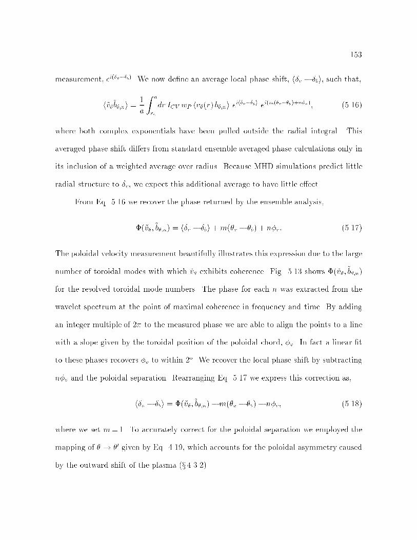
153

measurement, ei(vb). We now dene an average local phase shift, hv bi, such that,

h~v~b;ni = 1

a

Z a

ro

dr ICV wP hv(r) b;ni eihvbi ei(m(vb)+nv); (5.16)

where both complex exponentials have been pulled outside the radial integral. This

averaged phase shift diers from standard ensemble averaged phase calculations only in

its inclusion of a weighted average over radius. Because MHD simulations predict little

radial structure to v, we expect this additional average to have little eect

From Eq. 5.16 we recover the phase returned by the ensemble analysis,

(~v;~b;n) = hv bi +m(v b) + nv: (5.17)

The poloidal velocity measurement beautifully illustrates this expression due to the large

number of toroidal modes with which ~v exhibits coherence. Fig. 5.13 shows (~v;~b;n)

for the resolved toroidal mode numbers. The phase for each n was extracted from the

wavelet spectrum at the point of maximal coherence in frequency and time. By adding

an integer multiple of 2 to the measured phase we are able to align the points to a line

with a slope given by the toroidal position of the poloidal chord, v. In fact a linear t

to these phases recovers v to within 2o. We recover the local phase shift by subtracting

nv and the poloidal separation. Rearranging Eq. 5.17 we express this correction as,

hv bi = (~v;~b;n)m(v b) nv; (5.18)

where we set m=1. To accurately correct for the poloidal separation we employed the

mapping of ! 0 given by Eq. 4.19, which accounts for the poloidal asymmetry caused

by the outward shift of the plasma (x 4.3.2).

154

π

π/2

0

-π/2

-π6 8 10 12

toroidal mode number

δ v θ−

δ bθ,

n

Fig. 5.14.| The local phase of ~v and ~b;n for n=513 followingcorrection for the geometric separation of the measurements.The horizontal line at -144o represents a coherence weightedaveraged of the well resolved modes (lled circles).

5.3.3 Poloidal velocity uctuation phase

After correcting for the physical separation of the ~v and ~b;n measurements via Eq.

5.18, we obtain an average local phase of,

hv b;ni 140o; for 6 n 12: (5.19)

For poloidal velocity uctuations to contribute maximally to an equilibrium dynamo eld

implies a local phase, v br , of either 0 or . Taking into account the =2 phase shift

between ~br(r) and ~b(a), we obtain an optimal local phase shift, hv b;ni, of =2.

The measured local phase is \in between" =2 and indicating the presence of a

non-zero dynamo eld contribution from this product. However, more than half of the

measured ~v power is out of phase with ~br.

Because the poloidal chord measures uctuations where the mean magnetic eld is

primarily poloidal we expect the chord to be extremely sensitive to any ~vk uctuations.

155

One potential source for ~vk uctuations is the advection of an equilibrium vk gradient past

the line of sight by radial perturbations in the magnetic eld. Simple calculations yield

the phase and approximate amplitude of such uctuations. In a generalized geometry we

consider an equilibrium eld Bo = Boz perturbed by a radial magnetic eld, ~bx, yielding

a total magnetic eld given by,

B = Bo

z +

bxBo

ei(kyy+kzz+!t)x

: (5.20)

Integrating the eld line equation we obtain an approximate expression for the perturbed

x position of the mean eld,

~x ibxBokz

ei(kyy+kz z+!t): (5.21)

Now assuming that the parallel uid ow is constant along the eld line we obtain the

apparent velocity uctuation due to advection of that ow by bx as,

~vz = ~xrxvz =ibxBokz

@vz@x

ei(kyy+kzz+!t): (5.22)

This ~vz possesses the same wavenumber as the advecting ~bx but is phase shifted from ~bx

by =2 We may estimate the amplitude of such an eect in MST at an r=a = 0:6 as,

j~vj brBm

@v@(r=a)

(0:1)(10 km=s) = 1 km=s; (5.23)

This provides an order of magnitude estimate consistent with the measured ~v. Thus,

the ~v measurement may be a combination of uctuations due to parallel ow advection

which are =2 out of phase with ~br and a lesser contribution of perpendicular dynamo

uctuations which are in phase with ~br.

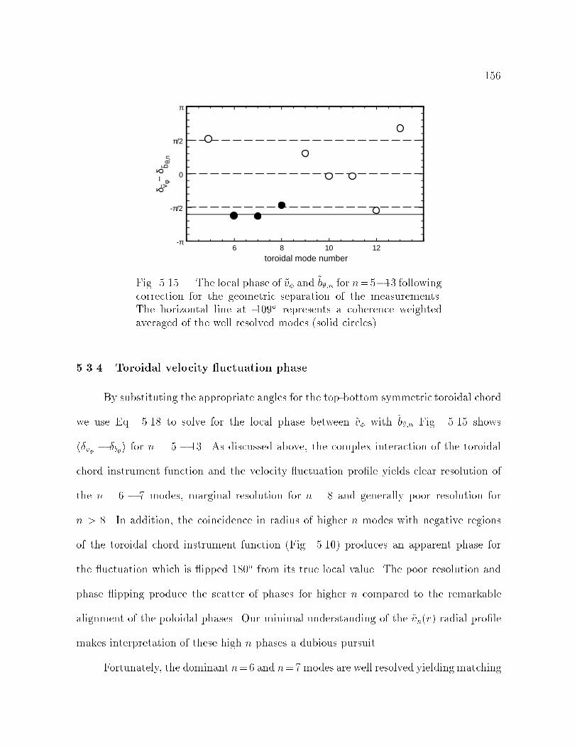
156

π

π/2

0

-π/2

-π6 8 10 12

toroidal mode number

δ v φ−

δ bθ,

n

Fig. 5.15.| The local phase of ~v and ~b;n for n=513 followingcorrection for the geometric separation of the measurements.The horizontal line at -109o represents a coherence weightedaveraged of the well resolved modes (solid circles).

5.3.4 Toroidal velocity uctuation phase

By substituting the appropriate angles for the top-bottom symmetric toroidal chord

we use Eq. 5.18 to solve for the local phase between ~v with ~b;n Fig. 5.15 shows

hv bi for n = 5 13. As discussed above, the complex interaction of the toroidal

chord instrument function and the velocity uctuation prole yields clear resolution of

the n = 6 7 modes, marginal resolution for n = 8 and generally poor resolution for

n > 8. In addition, the coincidence in radius of higher n modes with negative regions

of the toroidal chord instrument function (Fig. 5.10) produces an apparent phase for

the uctuation which is ipped 180o from its true local value. The poor resolution and

phase ipping produce the scatter of phases for higher n compared to the remarkable

alignment of the poloidal phases. Our minimal understanding of the ~vn(r) radial prole

makes interpretation of these high n phases a dubious pursuit.

Fortunately, the dominant n=6 and n=7 modes are well resolved yielding matching

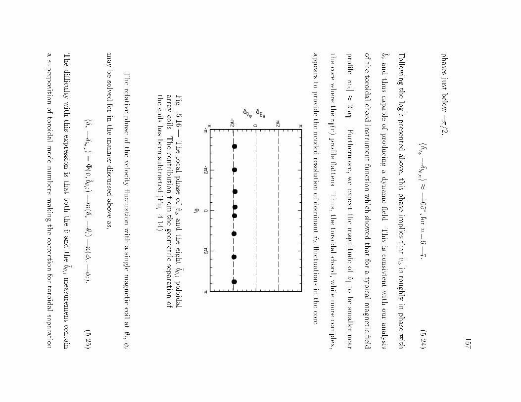
157

phases

justbelow

=2,

hv

b;n i

105

o;forn=6

7:(5.24)

Follow

ingthelogic

presen

tedabove,

thisphase

implies

that

~visrou

ghly

inphase

with

~brandthuscap

ableof

prod

ucin

gadynam

oeld

.Thisiscon

sistentwith

ouranaly

sis

ofthetoroid

alchord

instru

mentfunction

which

show

edthat

foratypical

magn

eticeld

pro

lejw

^ j2jw

k j.Furth

ermore,

weexpect

themagn

itudeof

~vkto

besm

allernear

thecore

where

thevk (r)

pro

le atten

s.Thus,thetoroid

alchord

,while

more

complex

,

appears

toprov

idetheneed

edresolu

tionofdom

inant~v^ uctu

ationsin

thecore.

π

π/20

-π/2-π

δvφ− δ

bθ

ππ/2

0-π/2

-π

θi

Fig.

5.16.|Thelocal

phase

of~vandtheeigh

t~b;ipoloid

alarray

coils.Thecon

tribution

fromthegeom

etricsep

arationof

thecoils

has

been

subtracted

(Fig.

4.14).

Therelativ

ephase

ofthevelocity

uctu

ationwith

asin

glemagn

eticcoil

ati ,i

may

besolv

edfor

inthemanner

discu

ssedabove

as,

hv

b;i i

=(~v; ~b

;i )

m(

v i )

n(

v i ):

(5.25)

Thediculty

with

thisexpression

isthat

both

the~vandthe~b;imeasu

rementcon

tain

asuperp

ositionof

toroidal

modenumbers

makingthecorrection

fortoroid

alsep

aration

158

ambiguous. We overcome this diculty by setting v i thereby mitigating that

dependency from Eq. 5.25. To do this we correlated the toroidal velocity uctuations

(v = 180o) with the ~b;i from the eight coils in the poloidal array at 180T (i = 177o).

The local phases which resulted from this measurement are shown in Fig. 5.16. Note

that the phases for each of the eight coils are extremely consistent, with an average value

of 85o We employed n = 6 in Eq. 5.25 to correct for the 3o toroidal separation. The

inclusion of power from higher n modes should alter this phase by no more than 5o.

This measurement together with the mode resolved correlation with ~b;n=6 and ~b;n=7

constitute strong evidence of ~v uctuations in the core regions of the MST phased such

as to produce a non-zero dynamo electric eld.

5.4 Radial Velocity Fluctuations

Throughout the preceding discussion we have denoted the ion velocity uctuation

measurements made along the poloidal and toroidal chords as ~v and ~v, respectively.

However, from our derivation of the full toroidal and poloidal chord instrument functions

(x 2.5.2), we know this to be an approximation. While the toroidal chord is minimally

sensitive to ~v and the poloidal chord is orthogonal to ~v, both chords exhibit sensitivity

to ~vr. This alone necessitates a separate measurement of ~vr in order to quantify the

potential contribution of ~vr to uctuations measured by the two chords. In addition, the

full cross product for the two parallel components of the dynamo eld are given by,

E = h~vr~bi h~v~bri; (5.26)

E = h~v~bri h~vr~bi: (5.27)

159

Thus, our ultimate goal of measuring the full h~v~bi dynamo electric eld clearly requires

measurement and correlation of ~vr.

To measure ~vr we constructed the large radial view port described in x 2.1 and

conducted an ensemble of low current discharges orienting one IDS view along the new

radial line of sight and positioning the second view along the traditional toroidal view

for direct comparison. This experiment produced two key results. First, the measured

power of ~vr is similar to that of the chord-averaged ~v. However, correcting for the sub-

stantial attenuation of ~v by the toroidal chord geometry we project a core ~v amplitude

23 times as large as ~vr. Second, ~vr exhibits extremely low coherence with the edge

magnetics, barely exceeding the coherence baseline in the tearing mode frequencies in

contrast to the robust coherence of ~v. These two results imply that while ~vr power may

contribute to the uctuation power reported above for the toroidal and poloidal chords,

that contribution should have little eect on the measured coherence and phase of the two

measured quantities. In addition, the absence of ~vr coherence implies that the dynamo

cross products, Eqs. 5.265.27, are dominated by the h~vbri and h~vbri terms.

5.4.1 A low noise measurement of ~vr

The radial view port was designed to maximize the light gathered by looking directly

through a 4 1/2 inch port. By employing an eight inch-diameter window as a vacuum

seal and a seven inch-diameter lens to focus light onto the lter monochromator, we

insured that the xed diameter of the port served as our limiting aperture. This design

produced light levels with the radial viewport which exceeded those of the toroidal view

by 50% (Fig. 5.17a). This enhanced light level reduced the intrinsic photon noise in the

emission proles of the radial view by 20% which then propagated directly to improved

160

0

50

100

150

200

250

300

0.00

0.05

0.10

0.15

0.20

-2 -1 0 1 2

time (ms)

A0

(bits

)χ2

A0

χ=

χr

χφ

A0,φA0,r

Fig. 5.17.| a) The ensembled amplitude of the tted Gaus-sian, A0, indicates the light collection of the radial port(solid) exceeds that of the toroidal port (grey) by 50%.b) This results in better ts and lower for the radial mea-surement.

nonlinear ts and a reduced (Fig. 5.17b). Ultimately the enhanced light levels for the

radial port should produce ~vr measurements with noise levels reduced from those of the

~v measurements taken concurrently.

In addition to cleaner ~v signals the radial chord exhibits a literally perfect instru-

ment function for the resolution of m=1 radial velocity uctuations (x 2.5.2). This con-

trasts sharply to the complex, spatially dependent toroidal instrument functions which

optimistically yield 50% attenuation, with more realistic estimates of 70% for the

dominant modes. Thus, this measurement compares the previously measured ~v to a less

noisy and more clearly resolved ~vr.

161

Pvφ=13 (km / s)2

Pδφ = 31(km / s)2

2.0

1.5

1.0

0.5

0.02.0

1.5

1.0

0.5

0.00 10 20 30 40 50

kHz

(km

/s)2

/kH

z(k

m/ s

)2/k

Hz

Pvr= 10(km / s)2

Pδr= 27 (km / s)2

a)

b)

Fig. 5.18.| The ensembled power spectra for a) ~v and b)~vr. Increased light levels decrease the measured noise oor(light) for ~vr compared to ~v. Following subtraction of thenoise oor slightly more uctuation power (dark) remains for~v than for ~vr. Integrated noise and uctuation powers areshown in the gures.

5.4.2 Modest, incoherent radial velocity uctuations

The ensembled power spectra of the measured ~v and ~vr are shown in Fig. 5.18. As

expected the noise oor for the ~v measurement exceeds the more cleanly illuminated ~vr

measurement. The toroidal velocity uctuation power above the noise oor is somewhat

greater than the corresponding radial uctuation power. However, some of P~v may

stem from secular contributions which should be largely absent from ~vr as the latter

exhibits little mean ow. Subtraction of the estimated secular power yields comparable

levels of measured uctuation power for the two components within the accuracy of the

measurement. Adjustments for the 23 fold attenuation of ~v by the toroidal chord, yield

estimates of ~v in the core which are 23 times larger than the perfectly resolved ~vr.

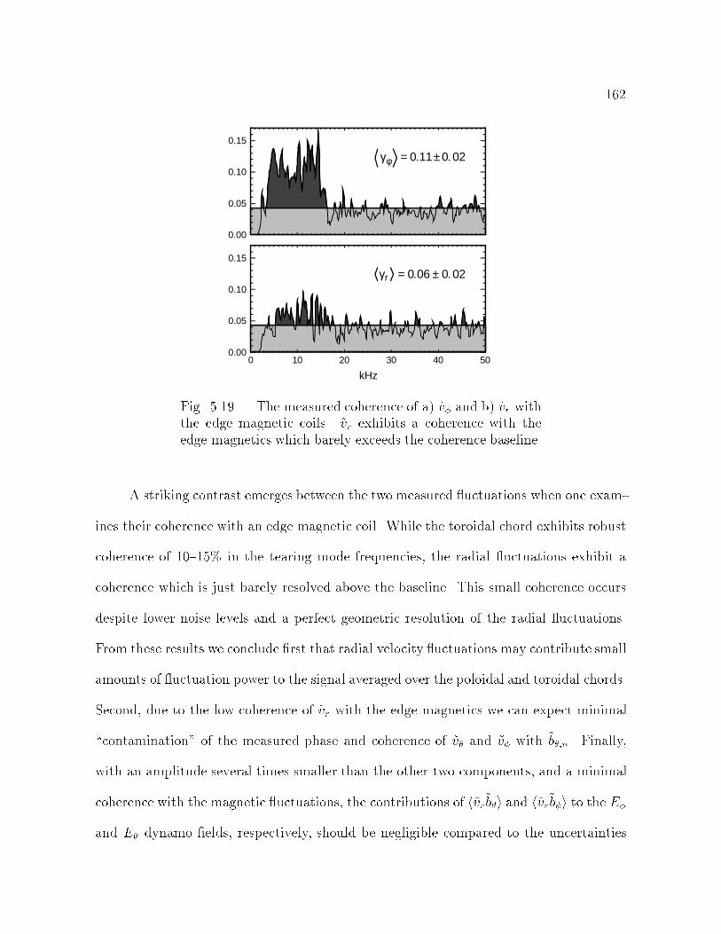
162

γφ = 0.11± 0.02

0.00

0.05

0.10

0.15

0 10 20 30 40 50

0.00

0.05

0.10

0.15

γr = 0.06 ± 0.02

kHz

Fig. 5.19.| The measured coherence of a) ~v and b) ~vr withthe edge magnetic coils. ~vr exhibits a coherence with theedge magnetics which barely exceeds the coherence baseline.

A striking contrast emerges between the two measured uctuations when one exam-

ines their coherence with an edge magnetic coil. While the toroidal chord exhibits robust

coherence of 1015% in the tearing mode frequencies, the radial uctuations exhibit a

coherence which is just barely resolved above the baseline. This small coherence occurs

despite lower noise levels and a perfect geometric resolution of the radial uctuations.

From these results we conclude rst that radial velocity uctuations may contribute small

amounts of uctuation power to the signal averaged over the poloidal and toroidal chords.

Second, due to the low coherence of ~vr with the edge magnetics we can expect minimal

\contamination" of the measured phase and coherence of ~v and ~v with ~b;n. Finally,

with an amplitude several times smaller than the other two components, and a minimal

coherence with the magnetic uctuations, the contributions of h~vr~bi and h~vr~bi to the E

and E dynamo elds, respectively, should be negligible compared to the uncertainties

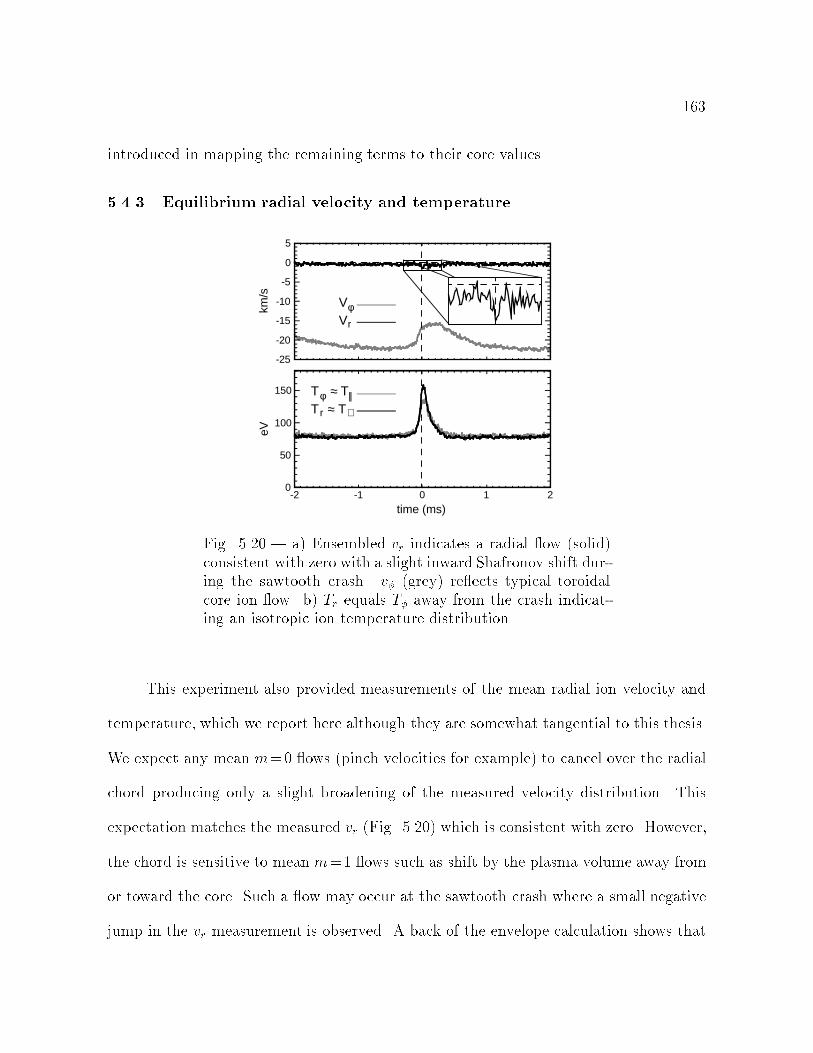
163

introduced in mapping the remaining terms to their core values.

5.4.3 Equilibrium radial velocity and temperature

-2 -1 0 1 2

time (ms)

0

50

100

150

-25

-20

-15

-10

-5

0

5

km/s

eV

Vr

Vφ

Tr ≈ T ⊥

Tφ ≈ T||

Fig. 5.20.| a) Ensembled vr indicates a radial ow (solid)consistent with zero with a slight inward Shafronov shift dur-ing the sawtooth crash. v (grey) re ects typical toroidalcore ion ow. b) Tr equals T away from the crash indicat-ing an isotropic ion temperature distribution.

This experiment also provided measurements of the mean radial ion velocity and

temperature, which we report here although they are somewhat tangential to this thesis.

We expect any mean m=0 ows (pinch velocities for example) to cancel over the radial

chord producing only a slight broadening of the measured velocity distribution. This

expectation matches the measured vr (Fig. 5.20) which is consistent with zero. However,

the chord is sensitive to mean m=1 ows such as shift by the plasma volume away from

or toward the core. Such a ow may occur at the sawtooth crash where a small negative

jump in the vr measurement is observed. A back of the envelope calculation shows that

164

this 500 m/s jump which extends 50 s corresponds to an inward shift of the plasma

of 3 cm. This is consistent with the expected relaxation of the Shafronov shift during

the crash.

The radial and toroidal ion temperatures exhibit identical values over most of the

sawtooth period consistent with an isotropic temperature distribution. Immediately be-

fore the crash both temperatures rise sharply together with no lag visible between T

and Tr. A dierence of 2030 eV occurs during the crash as Tr reaches 160 eV while

T plateaus at 130 eV. This dierence persists for less than 100 s at which point both

temperatures fall together back to their baseline value of 80 eV. This result contra-

dicts the measurements on the EXTRAP-T2 device (Sasaki, 1997) which showed strong

anisotropy between the T? and Tk of the majority ion species. Further measurements are

indicated to resolve this contradiction.

5.5 Lundquist Number Scaling

The extended runs at medium and high currents allowed three point Lundquist

number scalings of the velocity uctuations like those discussed in the previous chapter

for the magnetics. Fig. 5.21 shows h~v2i1

2 and h~v2i1

2 , in the three Lundquist number

regimes with the estimated noise baseline removed. The negative values seen after the

crash for the high S regime correspond to errors in our distribution of noise in time. As

with the magnetic uctuations the key eect of scaling is the decreased duty cycle of the

uctuations with baseline of the uctuations extending while the period of active uctu-

ation contracts. From this we expect the uctuation levels averaged over the sawtooth

to scale more strongly than either the baseline or the peak levels scale individually.

Normalizing the toroidal and poloidal uctuations by the Alvfen velocity we achieve

165

0

2

4

-4 -2 0 2ms

Low S

Medium S

High S

0

2

4

toro

idal

vel

ocity

fluc

tuat

ion

(km

/s)

0

2

4

0

2

4

-4 -2 0 2ms

Low S

Medium S

High S

0

2

4

polo

idal

vel

ocity

fluc

tuat

ion

(km

/s)

0

2

4

Fig. 5.21.| a) Toroidal (left) and b) poloidal (right) velocity uctuations forthe three Lundquist number settings. The estimated noise baselines have beenremoved and adjacent points have been binned every 0.5 ms. Error bars derivefrom the standard deviation of the points binned

the scalings shown in Fig. 5.22. The peak uctuation levels scale with slightly positive

exponents as,

max(~v) / S0:02; (5.28)

max(~v) / S0:07; (5.29)

(rst reported in Stoneking, 1997). This scaling is fairly consistent with the weak scaling

found for the peak levels of the magnetic uctuations of max (~b=Bo) / S0:02 (Eq. 4.20).

As expected, the uctuations averaged over the sawtooth scale more strongly than the

peak values due to the decreased uctuation duty cycle,

avg(~v) / S0:19; (5.30)

avg(~v) / S0:08: (5.31)

This also is consistent with the scaling of the magnetics for which we found, avg (~b=Bo) /

S0:08 (Eq. 4.21).

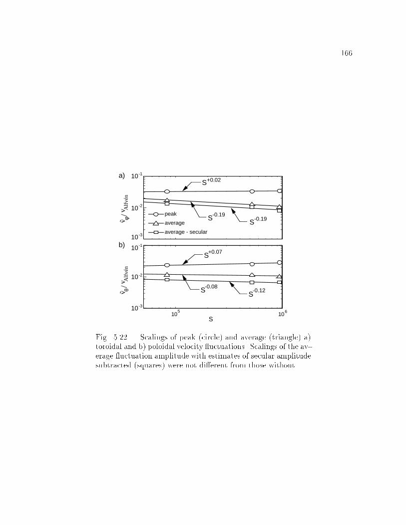
166

10-3

10-2

10-1

10-3

10-2

10-1

106105

S

a)

b)

S+0.02

S-0.19

S-0.19

S+0.07

S-0.08

S-0.12v

/vA

lfvé

nθ

peak

average

average - secular

v/v

Alf

vén

φ

Fig. 5.22.| Scalings of peak (circle) and average (triangle) a)toroidal and b) poloidal velocity uctuations. Scalings of the av-erage uctuation amplitude with estimates of secular amplitudesubtracted (squares) were not dierent from those without.

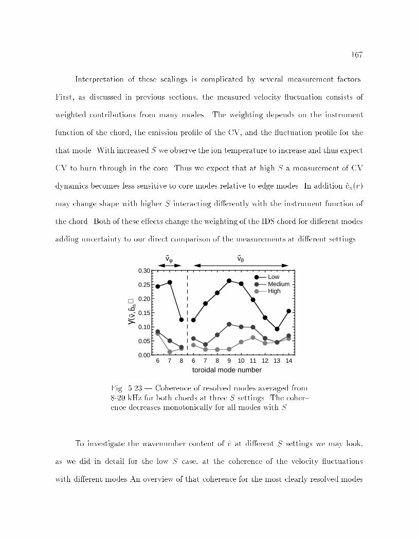
167

Interpretation of these scalings is complicated by several measurement factors.

First, as discussed in previous sections, the measured velocity uctuation consists of

weighted contributions from many modes. The weighting depends on the instrument

function of the chord, the emission prole of the CV, and the uctuation prole for the

that mode. With increased S we observe the ion temperature to increase and thus expect

CV to burn through in the core. Thus we expect that at high S a measurement of CV

dynamics becomes less sensitive to core modes relative to edge modes. In addition ~vn(r)

may change shape with higher S interacting dierently with the instrument function of

the chord. Both of these eects change the weighting of the IDS chord for dierent modes

adding uncertainty to our direct comparison of the measurements at dierent settings.

6 7 8 76 8 9 10 11 12 13 140.00

0.05

0.10

0.20

0.15

0.25

0.30LowMediumHigh

toroidal mode number

γv,

b n(

)

vφ vθ

Fig. 5.23.| Coherence of resolved modes averaged from8-20 kHz for both chords at three S settings. The coher-ence decreases monotonically for all modes with S.

To investigate the wavenumber content of ~v at dierent S settings we may look,

as we did in detail for the low S case, at the coherence of the velocity uctuations

with dierent modes An overview of that coherence for the most clearly resolved modes

168

is shown in Fig.5.23. Note that as anticipated, the relative content of various modes

does change with S with ~v containing fewer edge modes and ~v becoming exclusively

sensitive to n=6 uctuations. A more dramatic eect is the decreased coherence of the

measured velocity uctuations and all of the magnetic modes with increased S. Some of

the decrease stems from the increased noise levels in the IDS signal at higher currents

due to decreased emission levels of CV. However, this eect does not account for all of

observed decrease in coherence suggesting that the velocity uctuations may couple less

eciently to the magnetics at higher S. We will discuss this further when we examine

the scaling of the dynamo electric eld.

While the resolution of the local h~v ~bi phase suered at higher S due to

the low coherence, within the error no signicant variations in the phase were observed

between the dierent S ensembles. The up-down toroidal setup was not employed for

the medium and high current runs making a similar comparison of the local h~v ~bi

phase impossible.

References

Sasaki, K., P. Horling, T. Fall, J. H. Brzozowski, P. Brunsell, S. Hokin, E. Tennfors,J. Sallander, J. R. Drake, N. Inoue, J. Morikawa, Y. Ogawa, and Z. Yoshida(1997). Anistropy of ion temperature in a reversed-eld-pinch. Plasma Phys.Control. Fusion 39, 333338.

Stoneking, M. R., J. T. Chapman, D. J. Den Hartog, S. C. Prager, and J. S. Sar (1997).Experimental scaling of uctuations and connement with Lundquist number inthe RFP. Phys. Plasmas 5(4), 10041014.

169

6

The Balance of Ohm's Law

At the beginning of this thesis we demonstrated that in an RFP the mean currents and

the mean applied electric eld do not satisfy a linear parallel Ohm's law, leading to the

proposition of a ux surface averaged ~v ~b product providing this balance as,

hEik + h~v ~bik = hJik: (6.1)

In this chapter we examine the balance of this equation in the interior of MST in two

parts. First, we model hEik + h~v ~bik and hJik in Eq. 6.1 and estimate the size and

time behavior of the dynamo eld from their dierence. Second, we project our measured

h ~v~b;ni and h ~v~b;ni products into the core yielding empirical estimates of components

of h~v ~bi in the interior of MST. The key novel results of the chapter are summarized

here:

During the sawtooth crash the rapid relaxation of the current prole induces a

transient electric eld of tens of Volts/m which greatly exceeds both the applied

eld and the electric eld necessary to drive current in the plasma.

During the crash the dynamo term implied by the modeling would act to suppress

core current with a eld of 2040 Volts/m and drive edge current with a eld of

515 Volts/m

170

Away from the crash the inductance of the plasma opposes the resistive decay of

the equilibrium balancing Ohm's law within the 12 Volts/m precision of the

model.

From our measurement of h ~v~b;ni we estimate h ~v ~bri h~v~bi of 146 Volts/mat the crash and 1.00.4 Volts/m away from the crash in a direction to drive parallel

current at an r=a0.30.4.

From our measurement of h ~v~b;ni we estimate h ~v ~bri h~v~bi of 1.00.3 Volts/mat the crash and 0.140.05 Volts/m away from the crash with a small parallel

projection in a direction to drive parallel current at an r=a0.60.7.

Both dynamo products scale nearly as S1 due to the increasing incoherence of ~v

and ~b at the higher current regimes.

The modeling results provide new insights into the mean eld behavior, stressing the

importance of the plasma inductance over the sawtooth cycle. In addition, the h~v ~bi

measurements provide provocative evidence of dynamo activity in the core with a time

dependence and magnitude consistent with our expectations. However, substantial un-

certainties in the dynamo eld projected from measurements and that inferred from

modeling demonstrate the need for more sophisticated measurements of mean eld and

uctuating quantities before the numerical balance of Eq. 6.1 can be conclusively demon-

strated in MST.

This chapter contains two sections. The rst section evolves standard RFP equi-

librium models over the sawtooth to determine the dynamic mean-eld behavior of the

MST. The second section presents the measured uctuation products and describes the

correction factors employed to infer h ~v ~bri and h ~v ~bri in the core from the measured

h ~v~b;ni and h ~v~b;ni products.

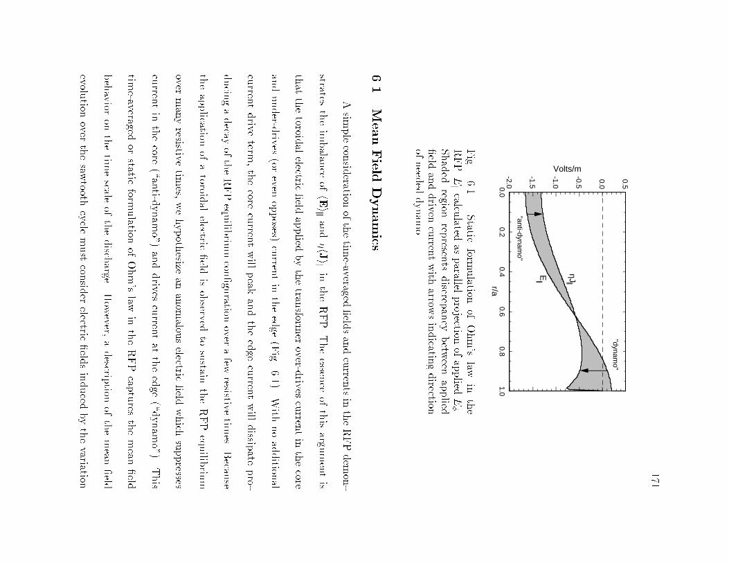
171

-2.0

-1.5

-1.0

-0.5

0.0

0.50.00.2

0.40.6

0.81.0

"anti-dynamo"

"dynamo"

r/a

Volts/mηJ||

E||

Fig.

6.1.|Static

formulation

ofOhm's

lawin

the

RFP.Ekcalcu

latedas

parallel

projection

ofapplied

E .

Shaded

regionrep

resents

discrep

ancy

betw

eenapplied

eld

anddriven

curren

twith

arrowsindicatin

gdirection

ofneed

eddynam

o.

6.1

MeanField

Dynamics

Asim

plecon

sideration

ofthetim

e-averagedeld

sandcurren

tsintheRFPdem

on-

stratestheimbalan

ceofhEi

kandhJi

kin

theRFP.Theessen

ceof

thisargu

mentis

that

thetoroid

alelectric

eld

applied

bythetran

sformer

over-drives

curren

tin

thecore

andunder-d

rives(or

evenopposes)

curren

tin

theedge

(Fig.

6.1).With

noaddition

al

curren

tdriv

eterm

,thecore

curren

twill

peak

andtheedge

curren

twill

dissip

atepro-

ducin

gadecay

oftheRFPequilib

riumcon

guration

overafew

resistivetim

es.Becau

se

theapplication

ofatoroid

alelectric

eld

isobserved

tosustain

theRFPequilib

rium

overmanyresistiv

etim

es,wehypoth

esizean

anom

alouselectric

eld

which

suppresses

curren

tin

thecore

(\anti-d

ynam

o")anddrives

curren

tat

theedge

(\dynam

o").This

time-averaged

orstatic

formulation

ofOhm'slaw

intheRFPcap

tures

themean

eld

behavior

onthetim

escale

ofthedisch

arge.How

ever,adescrip

tionof

themean

eld

evolution

overthesaw

toothcycle

mustcon

sider

electriceld

sinduced

bythevariation

172

of the magnetic eld in time. Our approach in this section will be to model the equilib-

rium magnetic eld from edge and global measurements at each point in time along the

sawtooth cycle. We may then solve for the mean electric elds in the plasma induced

by the external ux swing of the transformer and by the internal redistribution of ux

in the plasma. This modeling will yield very dierent mean eld behavior at and away

from the crash with equally dierent implications for the necessary dynamo eld. While

in our nal determination the dynamo eld necessary to balance a dynamic Ohm's law

behaves in a qualitatively similar fashion to that shown in Fig. 6.1, the sawtooth crash

compresses the duration and multiplies the magnitude of the necessary eld.

6.1.1 Cylindrical Modeling of the Equilibrium Magnetic Field

In the absence of current prole diagnostics we must rely on equilibriummodeling to

investigate mean-eld dynamics in MST. Below we describe simple cylindrical equilibrium

models of the current prole which we t to edge and global magnetic measurements.

The dynamics of the modeled current proles exhibit a suppression of core current and

attening of the current prole during the crash.

Models of the parallel current prole

We employed two simple models of (r) for this study: the \-model" and the

\Modied Bessel Function Model (MBFM)". Both specify the form of (r) with two

adjustable parameters: o, which species the parallel current on axis and a second

parameter which determines how rapidly the parallel current falls to zero at the plasma

edge. The MBFM holds (r) constant out to a \break radius", rb, at which point (r)

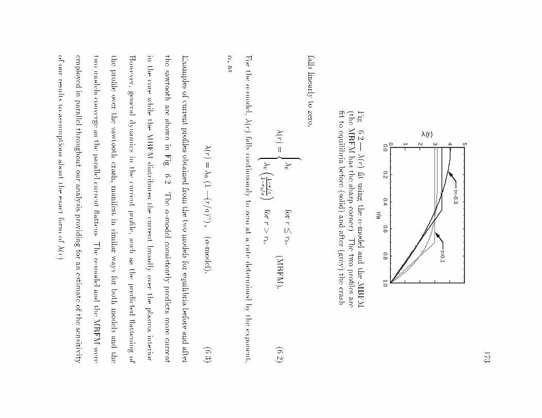
173

0.00.2

0.40.6

0.81.0

r/a

10 2 3 4 5

λ (r)

t=-0.3

t=0.1

Fig.

6.2.|(r)

tusin

gthe-m

odel

andtheMBFM

(theMBFM

has

thesharp

corner).

Thetwopro

lesare

tto

equilib

riabefore

(solid)andafter

(grey)thecrash

.

fallslinearly

tozero,

(r)

= 8>>><>>>:0

forr

rb ;

0

1r=a

1rb =a

forr>rb ;

(MBFM):

(6.2)

For

the-m

odel,

(r)

fallscon

tinuously

tozero

atarate

determ

ined

bytheexponent,

,as

(r)

=0(1

(r=a));

(-m

odel):

(6.3)

Exam

ples

ofcurren

tpro

lesobtain

edfrom

thetwomodels

forequilib

riabefore

andafter

thesaw

toothare

show

nin

Fig.

6.2.The-m

odel

consisten

tlypred

ictsmore

curren

t

inthecore

while

theMBFM

distrib

utes

thecurren

tbroad

lyover

theplasm

ainterior.

How

ever,gen

eraldynam

icsin

thecurren

tpro

le,such

asthepred

icted atten

ingof

thepro

leover

thesaw

toothcrash

,manifest

insim

ilarwaysfor

both

models

andthe

twomodels

converge

astheparallel

curren

t atten

s.The-m

odelandtheMBFM

were

employed

inparallel

throu

ghoutouranaly

sisprov

idingfor

anestim

ateofthesen

sitivity

ofourresu

ltsto

assumption

sabouttheexact

formof(r).

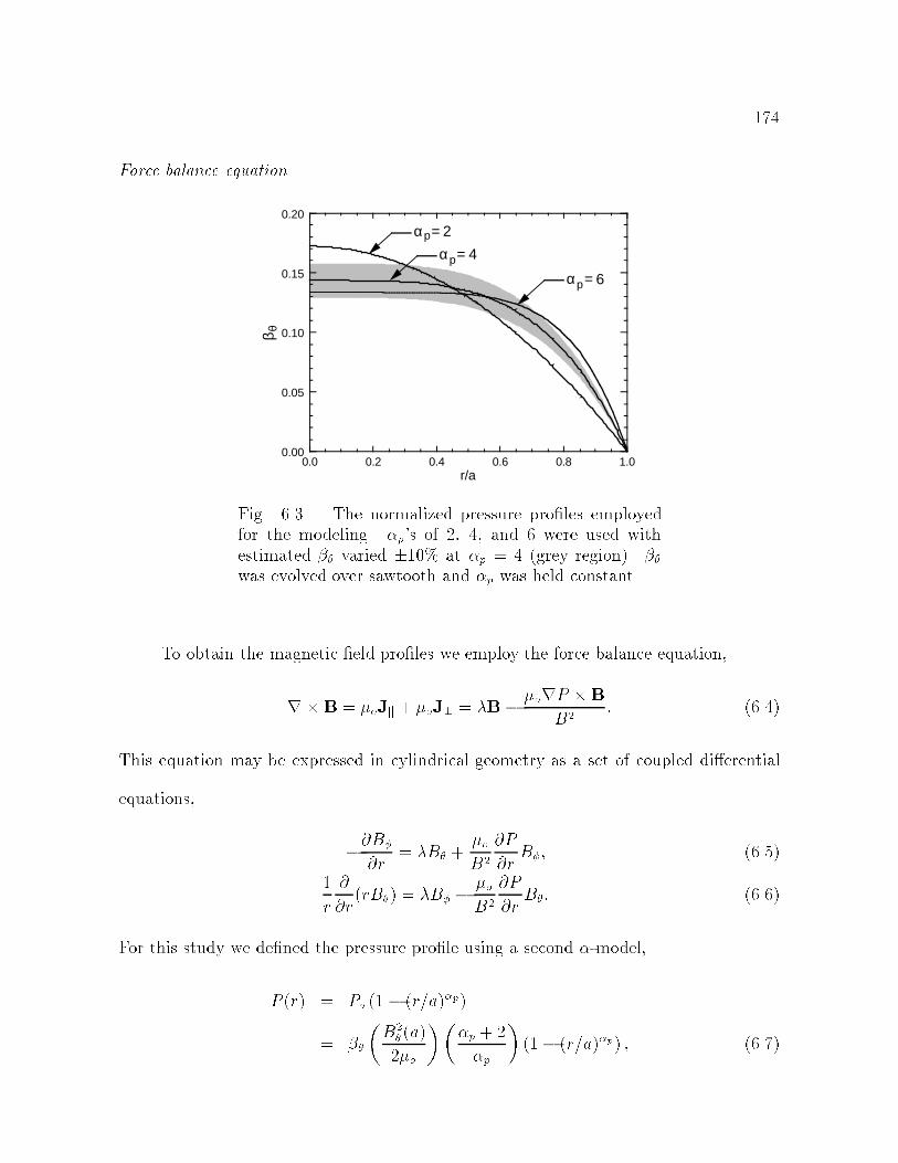
174

Force balance equation

αp= 2

0.00

0.05

0.10

0.15

0.20

0.0 0.2 0.4 0.6 0.8 1.0

β θ

r/a

αp= 4

αp= 6

Fig. 6.3.| The normalized pressure proles employedfor the modeling. p's of 2, 4, and 6 were used withestimated varied 10% at p = 4 (grey region). was evolved over sawtooth and p was held constant.

To obtain the magnetic eld proles we employ the force balance equation,

rB = oJk + oJ? = B orP B

B2: (6.4)

This equation may be expressed in cylindrical geometry as a set of coupled dierential

equations,

@B

@r= B +

oB2

@P

@rB; (6.5)

1

r

@

@r(rB) = B o

B2

@P

@rB: (6.6)

For this study we dened the pressure prole using a second -model,

P (r) = Po (1 (r=a)p)

=

B2 (a)

2o

p + 2

p

(1 (r=a)p) ; (6.7)

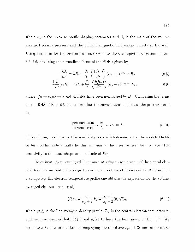
175

where p is the pressure prole shaping parameter and is the ratio of the volume

averaged plasma pressure and the poloidal magnetic eld energy density at the wall.

Using this form for the pressure we may evaluate the diamagnetic correction in Eqs.

6.56.6, obtaining the normalized forms of the PDE's given by,

@B

@r= B

2

B2 (a)

B2

(p + 2) rp1 B; (6.8)

1

r

@

@r(rB) = B +

2

B2 (a)

B2

(p + 2) rp1 B; (6.9)

where r=a! r, a! and all elds have been normalized by Bo. Comparing the terms

on the RHS of Eqs. 6.86.9, we see that the current term dominates the pressure term

as,

pressure term

current term

5 102: (6.10)

This ordering was borne out by sensitivity tests which demonstrated the modeled elds

to be modied substantially by the inclusion of the pressure term but to have little

sensitivity to the exact shape or magnitude of P (r).

To estimate we employed Thomson scattering measurements of the central elec-

tron temperature and line averaged measurements of the electron density. By assuming

a completely at electron temperature prole one obtains the expression for the volume

averaged electron pressure of,

hPeiV =p

p + 2Po =

p + 1

p + 2hneilTe0; (6.11)

where hneil is the line averaged density prole, Te0 is the central electron temperature,

and we have assumed both Pe(r) and ne(r) to have the form given by Eq. 6.7. We

estimate a Pi in a similar fashion employing the chord-averaged IDS measurements of

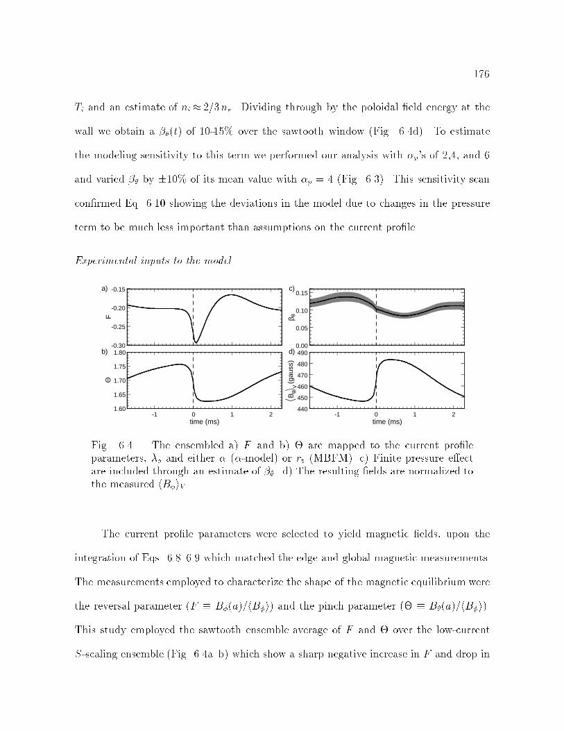
176

Ti and an estimate of ni 2=3ne. Dividing through by the poloidal eld energy at the

wall we obtain a (t) of 10-15% over the sawtooth window (Fig. 6.4d). To estimate

the modeling sensitivity to this term we performed our analysis with p's of 2,4, and 6

and varied by 10% of its mean value with p = 4 (Fig. 6.3). This sensitivity scan

conrmed Eq. 6.10 showing the deviations in the model due to changes in the pressure

term to be much less important than assumptions on the current prole.

Experimental inputs to the model

-0.30

-0.25

-0.20

-0.15

1.80

1.75

1.70

1.65

1.60

0.15

0.10

0.05

0.00490

480

470

460

450

440

Bφ

V(g

auss

)β θF

Θ

a)

b)

c)

d)

-1 0 1 2time (ms)

-1 0 1 2time (ms)

Fig. 6.4.| The ensembled a) F and b) are mapped to the current proleparameters, o and either (-model) or rb (MBFM). c) Finite pressure eectare included through an estimate of . d) The resulting elds are normalized tothe measured hBiV .

The current prole parameters were selected to yield magnetic elds, upon the

integration of Eqs. 6.86.9 which matched the edge and global magnetic measurements.

The measurements employed to characterize the shape of the magnetic equilibrium were

the reversal parameter (F B(a)=hBi) and the pinch parameter ( B(a)=hBi).

This study employed the sawtooth ensemble average of F and over the low-current

S-scaling ensemble (Fig. 6.4ab) which show a sharp negative increase in F and drop in

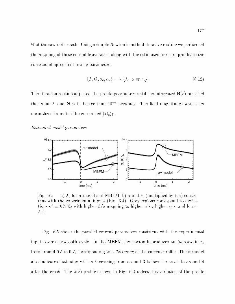
177

at the sawtooth crash. Using a simple Newton's method iterative routine we performed

the mapping of these ensemble averages, along with the estimated pressure prole, to the

corresponding current prole parameters,

fF;; ; pg =) f0; or rbg: (6.12)

The iteration routine adjusted the prole parameters until the integrated B(r) matched

the input F and with better than 105 accuracy. The eld magnitudes were then

normalized to match the ensembled hBiV .

Estimated model parameters

α,10

r b

λ o

2.5

3.0

3.5

4.0

4.5

0

2

4

6

8

MBFM

α− modelMBFM

α − model

-1 0 1 2time (ms)

-1 0 1 2time (ms)

a) b)

Fig. 6.5.| a) o for -model and MBFM, b) and rb (multiplied by ten) consis-tent with the experimental inputs (Fig. 6.4). Grey regions correspond to devia-tions of 10% with higher 's mapping to higher 's , higher rb's, and lowero's.

Fig. 6.5 shows the parallel current parameters consistent with the experimental

inputs over a sawtooth cycle. In the MBFM the sawtooth produces an increase in rb

from around 0.5 to 0.7, corresponding to a attening of the current prole. The -model

also indicates attening with increasing from around 3 before the crash to around 4

after the crash. The (r) proles shown in Fig. 6.2 re ect this variation of the prole

178

about the sawtooth. Both models indicate a suppression of parallel current during the

crash. As noted above the -model predicts higher o for the steep proles, though the

o values of the two models converge as the proles atten. This results in a o for

the -model with greater apparent suppression of core current at the sawtooth crash.

With higher estimates of both models predicted lower values of 0 and atter current

proles, although the eects of pressure were minimal. All of the electric and magnetic

eld sawtooth crash dynamics discussed below may be completely understood as either

a manifestation of or a response to the current prole attening described by these

parameters.

6.1.2 Mean Field Electrodynamics

Modeling of the equilibrium over the sawtooth cycle enables us to investigate the

evolution of the magnetic ux and to calculate the electric eld induced by changes in that

ux. Below we qualitatively examine the dynamics of the equilibriummagnetic eld and

the redistribution of magnetic ux during the sawtooth crash. The two key phenomena

observed are the loss of poloidal ux in the plasma core and the generation of toroidal

ux in the mid-region of the plasma. The latter is partially oset by a slight loss of

toroidal ux in the core and a transient increase in negative toroidal ux at the edge.

By calculating the time derivative of the integrated ux we obtain estimates of induced

electric elds with peak amplitude of tens of Volts/m during the crash. Below we rst

describe the evolution of the magnetic eld and then describe the electric elds induced

by these changes. Again the eld described here results from models of the current prole

which are constrained by edge measurements but is in no way a unique solution to the

parallel current in the MST. By pursuing two models of the parallel current we hope to

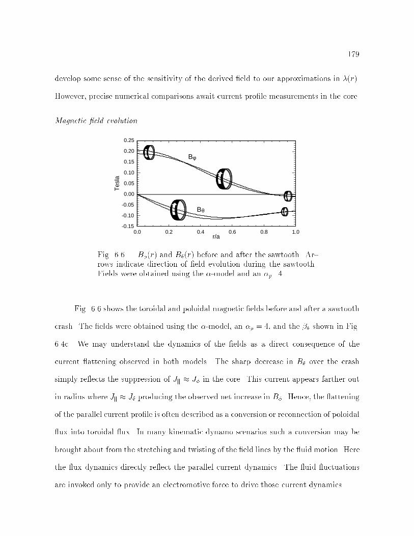
179

develop some sense of the sensitivity of the derived eld to our approximations in (r).

However, precise numerical comparisons await current prole measurements in the core.

Magnetic eld evolution

r/a

Tes

la

0.25

0.20

0.15

0.10

0.05

0.00

-0.05

-0.10

-0.150.0 0.2 0.4 0.6 0.8 1.0

Bφ

Bθ

Fig. 6.6.| B(r) and B(r) before and after the sawtooth. Ar-rows indicate direction of eld evolution during the sawtooth.Fields were obtained using the -model and an p=4.

Fig. 6.6 shows the toroidal and poloidal magnetic elds before and after a sawtooth

crash. The elds were obtained using the -model, an p = 4, and the shown in Fig.

6.4c. We may understand the dynamics of the elds as a direct consequence of the

current attening observed in both models. The sharp decrease in B over the crash

simply re ects the suppression of Jk J in the core. This current appears farther out

in radius where Jk J producing the observed net increase in B. Hence, the attening

of the parallel current prole is often described as a conversion or reconnection of poloidal

ux into toroidal ux. In many kinematic dynamo scenarios such a conversion may be

brought about from the stretching and twisting of the eld lines by the uid motion. Here

the ux dynamics directly re ect the parallel current dynamics. The uid uctuations

are invoked only to provide an electromotive force to drive those current dynamics.

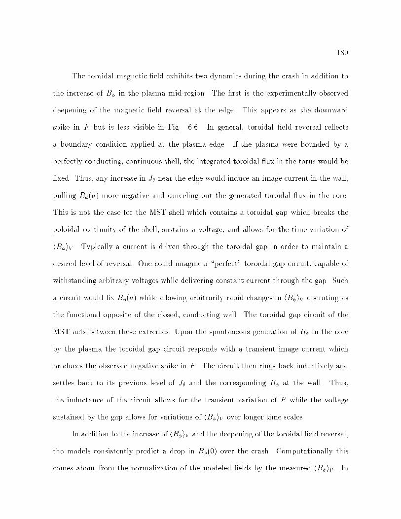
180

The toroidal magnetic eld exhibits two dynamics during the crash in addition to

the increase of B in the plasma mid-region. The rst is the experimentally observed

deepening of the magnetic eld reversal at the edge. This appears as the downward

spike in F but is less visible in Fig. 6.6. In general, toroidal eld reversal re ects

a boundary condition applied at the plasma edge. If the plasma were bounded by a

perfectly conducting, continuous shell, the integrated toroidal ux in the torus would be

xed. Thus, any increase in J near the edge would induce an image current in the wall,

pulling B(a) more negative and canceling out the generated toroidal ux in the core.

This is not the case for the MST shell which contains a toroidal gap which breaks the

poloidal continuity of the shell, sustains a voltage, and allows for the time variation of

hBiV . Typically a current is driven through the toroidal gap in order to maintain a

desired level of reversal. One could imagine a \perfect" toroidal gap circuit, capable of

withstanding arbitrary voltages while delivering constant current through the gap. Such

a circuit would x B(a) while allowing arbitrarily rapid changes in hBiV operating as

the functional opposite of the closed, conducting wall. The toroidal gap circuit of the

MST acts between these extremes. Upon the spontaneous generation of B in the core

by the plasma the toroidal gap circuit responds with a transient image current which

produces the observed negative spike in F . The circuit then rings back inductively and

settles back to its previous level of J and the corresponding B at the wall. Thus,

the inductance of the circuit allows for the transient variation of F while the voltage

sustained by the gap allows for variations of hBiV over longer time scales.

In addition to the increase of hBiV and the deepening of the toroidal eld reversal,

the models consistently predict a drop in B(0) over the crash. Computationally this

comes about from the normalization of the modeled elds by the measured hBiV . In

181

essence the measured increase in hBiV is not great enough to account for the modeled

increase in B in the plasma mid-region even with the jump in negative toroidal ux

at the edge. However, the dimensionless mapping of fF;g ) fo; g x the shape of

the B prole. Thus, the normalization reduces the overall magnitude of B to match

the integrated toroidal ux from the models to the measured toroidal ux integrated

over the plasma volume while maintaining the prole shape. This normalization results

in the predicted dip in B(0) as well as an overall decrease in the mean magnetic eld

energy. While we have no experimental information to conrm or contradict this modeled

behavior of B(0), the drop perhaps indicates the diculties of integrating approximate

models, bound by edge measurements, to predict the behavior of elds near the core.

One can imagine slight modications to the modeling of (r) which might distribute

current dierently to match the edge measurements while holding B(0) constant. This

diculty highlights the need for core current prole measurements to further constrain

the modeling of (r). In the mean time it may be an interesting exercise to explore the

behavior of three parameter (r) models with the a priori condition of constant B(0).

Redistribution of magnetic ux

To examine the redistribution of magnetic ux more carefully we dene the radial

derivative of the toroidal and poloidal magnetic ux as,

d

dr= 2RoB; (6.13)

d

dr= 2rB; (6.14)

where, Ro is the major radius of the torus. Fig. 6.7 shows a contour plot of these deriva-

tives where for each radius the average value of d=dr or d=dr over the sawtooth has

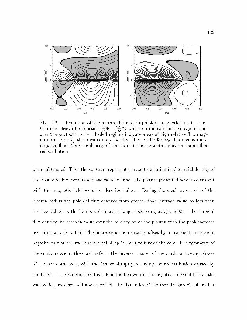
182

-1

0

1

2

time

(ms)

0.0 0.2 0.4 0.6 0.8 1.0

r/a

a)

-1

0

1

2

time

(ms)

0.0 0.2 0.4 0.6 0.8 1.0

r/a

b)

Fig. 6.7.| Evolution of the a) toroidal and b) poloidal magnetic ux in time.Contours drawn for constant d

dr h d

dri where h i indicates an average in time

over the sawtooth cycle. Shaded regions indicate areas of high relative ux mag-nitudes. For this means more positive ux, while for this means morenegative ux. Note the density of contours at the sawtooth indicating rapid uxredistribution.

been subtracted. Thus the contours represent constant deviation in the radial density of

the magnetic ux from its average value in time. The picture presented here is consistent

with the magnetic eld evolution described above. During the crash over most of the

plasma radius the poloidal ux changes from greater than average value to less than

average values, with the most dramatic changes occurring at r=a 0:3. The toroidal

ux density increases in value over the mid-region of the plasma with the peak increase

occurring at r=a 0:6. This increase is momentarily oset by a transient increase in

negative ux at the wall and a small drop in positive ux at the core. The symmetry of

the contours about the crash re ects the inverse natures of the crash and decay phases

of the sawtooth cycle, with the former abruptly reversing the redistribution caused by

the latter. The exception to this rule is the behavior of the negative toroidal ux at the

wall which, as discussed above, re ects the dynamics of the toroidal gap circuit rather

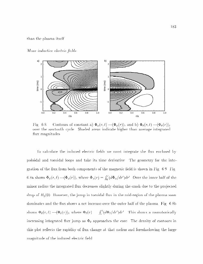
183

than the plasma itself.

Mean inductive electric elds

-1

0

1

2

time

(ms)

0.0 0.2 0.4 0.6 0.8 1.0

r/a

a)

-1

0

1

2

time

(ms)

0.0 0.2 0.4 0.6 0.8 1.0

r/a

b)

Fig. 6.8.| Contours of constant a) (r; t) h(r)it and b) (r; t) h(r)itover the sawtooth cycle. Shaded areas indicate higher than average integrated ux magnitudes.

To calculate the induced electric elds we must integrate the ux enclosed by

poloidal and toroidal loops and take its time derivative. The geometry for the inte-

gration of the ux from both components of the magnetic eld is shown in Fig. 6.9. Fig.

6.8a shows (r; t) h(r)it where (r) =R r0 (d=dr

0)dr0. Over the inner half of the

minor radius the integrated ux decreases slightly during the crash due to the projected

drop of B(0). However, the jump in toroidal ux in the mid-region of the plasma soon

dominates and the ux shows a net increase over the outer half of the plasma. Fig. 6.8b

shows (r; t) h(r)it where (r) =R ar(d=dr

0)dr0. This shows a monotonically

increasing integrated ux jump as approaches the core. The density of contours in

this plot re ects the rapidity of ux change at that radius and foreshadowing the large

magnitude of the induced electric eld.

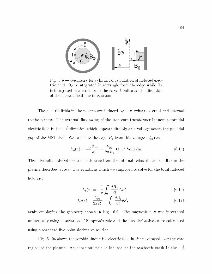
184

φ

r

a

lθ

Bθ

θl Bφφ,a r

Fig. 6.9.| Geometry for cylindrical calculation of induced elec-tric eld. is integrated in rectangle from the edge while

is integrated in a circle from the core. l indicates the directionof the electric eld line integration.

The electric elds in the plasma are induced by ux swings external and internal

to the plasma. The external ux swing of the iron core transformer induces a toroidal

electric eld in the direction which appears directly as a voltage across the poloidal

gap of the MST shell. We calculate the edge E from this voltage (Vpg) as,

E(a) = dext

dt=

Vpg2Ro

1:7 Volts/m: (6.15)

The internally induced electric elds arise from the internal redistributions of ux in the

plasma described above. The equations which we employed to solve for the total induced

eld are,

E(r) = 1

r

Z r

0

dB

dtr0dr0; (6.16)

E(r) =Vpg2Ro

Z a

r

dB

dtdr0; (6.17)

again employing the geometry shown in Fig. 6.9. The magnetic ux was integrated

numerically using a variation of Simpson's rule and the ux derivatives were calculated

using a standard ve-point derivative routine.

Fig. 6.10a shows the toroidal inductive electric eld in time averaged over the core

region of the plasma. An enormous eld is induced at the sawtooth crash in the

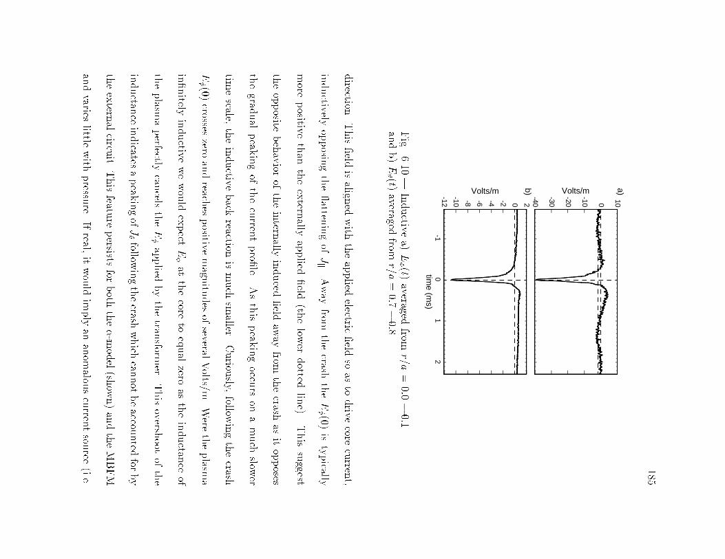
185

100

-10

-20

-30

-4020-2-4-6-8

-10

-12-1

01

2tim

e (ms)

Volts/m Volts/m

a)b)

Fig.

6.10.|Inductiv

ea)E (t)

averagedfrom

r=a=0:0

0:1andb)E (t)

averagedfrom

r=a=0:7

0:8.

direction

.Thiseld

isalign

edwith

theapplied

electriceld

soas

todriv

ecore

curren

t,

inductively

opposin

gthe atten

ingofJk .

Away

fromthecrash

theE (0)

istypically

more

positiv

ethan

theextern

allyapplied

eld

(thelow

erdotted

line).

This

suggest

theopposite

behavior

oftheintern

allyinduced

eld

away

fromthecrash

asitopposes

thegrad

ual

peak

ingof

thecurren

tpro

le.Asthispeak

ingoccu

rson

amuch

slower

timescale,

theinductive

back

reactionismuch

smaller.

Curiou

sly,follow

ingthecrash

E (0)

crosseszero

andreach

espositiv

emagn

itudesofseveral

Volts/m

.Were

theplasm

a

innitely

inductive

wewould

expect

Eat

thecore

toequal

zeroas

theinductan

ceof

theplasm

aperfectly

cancels

theEapplied

bythetran

sformer.

Thisoversh

ootof

the

inductan

ceindicates

apeak

ingofJfollow

ingthecrash

which

cannot

beaccou

nted

forby

theextern

alcircu

it.Thisfeatu

repersists

forboth

the-m

odel(sh

own)andtheMBFM

andvaries

littlewith

pressu

re.Ifreal,

itwould

implyan

anom

alouscurren

tsou

rce(i.e.

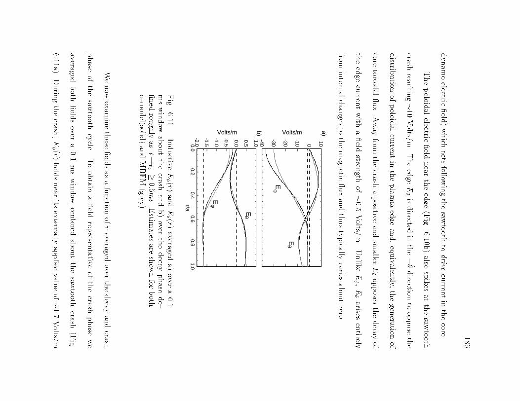
186

dynam

oelectric

eld

)which

actsfollow

ingthesaw

toothto

drivecurren

tin

thecore.

Thepoloid

alelectric

eld

near

theedge

(Fig.

6.10b)also

spikes

atthesaw

tooth

crashreach

ing

10Volts/m

.TheedgeEisdirected

inthe

direction

tooppose

the

distrib

ution

ofpoloid

alcurren

tin

theplasm

aedge

and,equivalen

tly,thegen

erationof

coretoroid

al ux.Away

fromthecrash

apositive

andsm

allerEopposes

thedecay

of

theedge

curren

twith

aeld

strength

of0.5

Volts/m

.Unlike

E ,Earises

entirely

fromintern

alchanges

tothemagn

etic uxandthustypically

variesaboutzero.

100

-10

-20

-30

-401.0

0.0

-1.0

-2.0

0.5

-0.5

-1.5

0.20.0

0.40.6

0.81.0

r/a

Volts/m Volts/m

a)b)

Eθ

Eφ

Eθ

Eφ

Fig.

6.11.|Inductive

E (r)

andE (r)

averageda)

overa0.1

mswindow

aboutthecrash

andb)over

thedecay

phase

de-

ned

roughly

asjttc j

0:5ms.

Estim

atesare

show

nfor

both

-m

odel(solid

)andMBFM

(grey).

Wenow

exam

inethese

eld

sas

afunction

ofraveraged

overthedecay

andcrash

phase

ofthesaw

toothcycle.

Toobtain

aeld

represen

tativeof

thecrash

phase

we

averagedboth

eld

sover

a0.1

mswindow

centered

aboutthesaw

toothcrash

(Fig.

6.11a).Durin

gthecrash

,E (r)

hold

snear

itsextern

allyapplied

valueof

1.7Volts/m

187

in the outer half of the plasma. Over the inner half of the plasma the eld grows rapidly

peaking at a value of 30 Volts/m at r = 0. As discussed above, this enormous induced

eld is aligned with the externally applied eld in the direction to drive current in the

core and oppose the redistribution of that current to the plasma edge. E(r) over the

inner half of the plasma acts to drive current opposing the loss of toroidal ux in the

very core of the plasma. At mid-radius E(r) ips sign as the generation of ux in the

mid-region of the plasma overtakes the loss in the core for a net increase in (r). E

opposes the increase Jk J over the outer region of the plasma exhibiting a nite value

at the plasma edge. In a check of model consistency we conrmed that with excellent

accuracy this edge poloidal electric eld was given by, E(a) = Vtg=2a, where Vtg is the

ensembled toroidal gap voltage.1

By averaging the elds for jt tcj 0:5 ms we recover the typical behavior of

E(r) during the decay phase of the sawtooth cycle. E(r) remains close to its externally

applied value over the outer region of the plasma and then decreases in magnitude near

the core as the inductance of the plasma opposes the resistive peaking of Jk. Likewise,

E(r) inductively opposes the dissipation of edge poloidal current (or, equivalently, core

toroidal ux) over the outer region of the plasma. This behavior matches what might be

expected of an RFP equilibrium decaying slowly in time. The signicantly diminished

eld magnitudes simply re ect the slower time scales of the ux changes during the decay

phase.

1This agreement conrms the absence of errors in the conversion by analog integrators of the measuredVtg to the stored hBiV signal, the subsequent normalization of the modeled B(r) by hBiV , thenumerical integration of B(r) to recover and the dierentiation in time of the ux yielding, nally,the correct E(a). While physically uninteresting, this loop eectively absolves our modeling of severalpotential sources of numerical error.

188

6.1.3 Resistive Current Dissipation

The task of modeling the resistive dissipation term in Ohm's law over the sawtooth

is comparatively simple with predicted dynamics over the crash which are comparatively

modest. Below we describe our estimation of the plasma resistivity from central electron

temperatures measured with Thomson scattering and Zeff inferred from central chord

averaged Bremsstrahlung measurements. We then multiply by Jk determined from

the cylindrical modeling to estimate the parallel electric eld necessary to drive modeled

current. We nd that Jk ranges from 2 Volts/m away from the sawtooth crash to 6

Volts/m at the crash with the increase due entirely to the spike in plasma resistivity.

The uncertainties in the estimated prole and magnitude of Jk are small compared to

the induced elds during the crash and thus have little impact on the implied dynamo

elds. Away from the crash these uncertainties will dominate our calculation.

Calculation of resistivity

The electron temperature was measured in the core by a Thomson scattering system

capable of a single laser re every discharge. We ran the system along a central chord

for 50 shots in the low current ensemble, triggering the laser to re at dierent times

relative to sawteeth in the at-top region of the discharge. By binning the photon counts

from neighboring measurements relative to the sawtooth crash time we were able to

reconstruct a coarse time evolution of the central electron temperature. Fig. 6.12 shows a

smoothed version of our estimated Te(t) along with a measurement uncertainty of 15%.

Similarmeasurements at other radii suggest an extremely at electron temperature prole

189

200

150

100

50

0 0

2

4

6

8

10

12

10

8

6

4

2

0-1 0 1 2

Zeff

Te

(eV

)η s

pitz

er( 1

0-6Ω

-m)

time (ms)

a)

b)

Fig. 6.12.| a) The central electron temperature,Te, estimated from single point Thomson scatteringmeasurements and Zeff estimated from chord aver-aged Bremsstrahlung measurements. b) Spitzer re-sistivity calculated using these values.

motivating the somewhat arbitrary modeling of the electron temperature prole as,

Te(r) = Te(0)(1 (Te(a)=Te(0) + 1)8); (6.18)

where we set Te(a)=Te(0) = 0:05.

To characterize Zeff we collected bremsstrahlung radiation which are mostly free

from contamination by neighboring spectral lines in the NIR and visible. Unfortunately,

these detectors were not absolutely calibrated at the time of the measurement. However,

by averaging the emitted radiation over the low, medium, and high current ensembles we

could calculate a relative Zeff as a function of time and current regime. Normalizing the

relative Zeff by the lowest measured value which occurred during the high current run

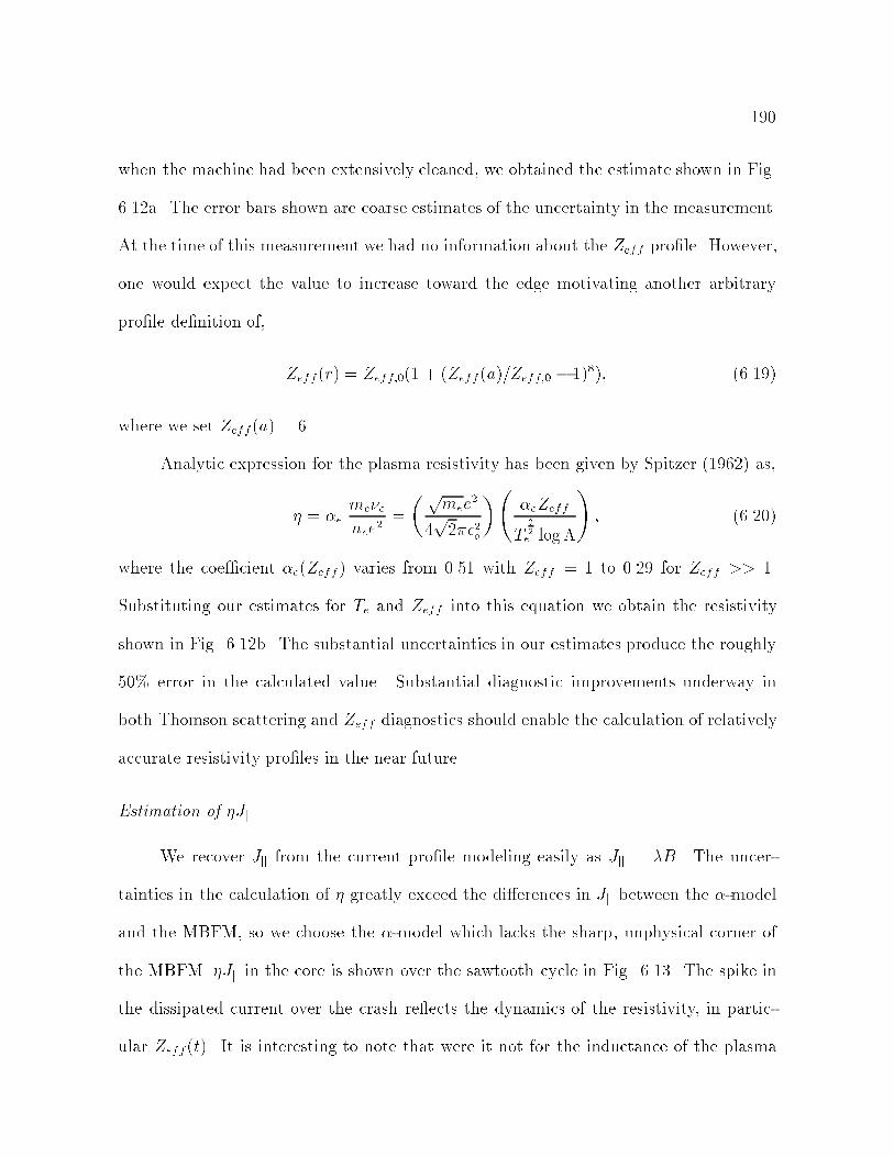
190

when the machine had been extensively cleaned, we obtained the estimate shown in Fig.

6.12a. The error bars shown are coarse estimates of the uncertainty in the measurement.

At the time of this measurement we had no information about the Zeff prole. However,

one would expect the value to increase toward the edge motivating another arbitrary

prole denition of,

Zeff (r) = Zeff;0(1 + (Zeff (a)=Zeff;0 1)8); (6.19)

where we set Zeff (a) = 6.

Analytic expression for the plasma resistivity has been given by Spitzer (1962) as,

= emeenee2

=

pmee

2

4p22o

eZeff

T3

2

e log

!; (6.20)

where the coecient e(Zeff ) varies from 0.51 with Zeff = 1 to 0.29 for Zeff >> 1.

Substituting our estimates for Te and Zeff into this equation we obtain the resistivity

shown in Fig. 6.12b. The substantial uncertainties in our estimates produce the roughly

50% error in the calculated value. Substantial diagnostic improvements underway in

both Thomson scattering and Zeff diagnostics should enable the calculation of relatively

accurate resistivity proles in the near future.

Estimation of Jk

We recover Jk from the current prole modeling easily as Jk = B. The uncer-

tainties in the calculation of greatly exceed the dierences in Jk between the -model

and the MBFM, so we choose the -model which lacks the sharp, unphysical corner of

the MBFM. Jk in the core is shown over the sawtooth cycle in Fig. 6.13. The spike in

the dissipated current over the crash re ects the dynamics of the resistivity, in partic-

ular Zeff (t). It is interesting to note that were it not for the inductance of the plasma

191

0-2-4-6-1

01

2

Volts/m

time (m

s)

Fig.

6.13.|Theestim

atedJk (0;t)

usin

gtheresistiv

ityshow

nin

Fig.

6.12bandthecurren

tderiv

edfrom

the-m

odel.

prod

ucin

gthelarge

electriceld

sdiscu

ssedabove,

thisenhanced

resistivity

durin

gthe

crashwould

bemore

than

enough

toaccou

ntfor

thesuppression

ofcurren

tin

thecore.

Ofcou

rse,such

aneect

could

not

besim

ilarlyinvoked

toexplain

theincreased

curren

t

attheedge

durin

gthecrash

.

0-1-2-3-4-50.00.2

0.40.6

0.81.0

Volts/m

r/a

Fig.

6.14.|Pro

leofJkdurin

g(solid

)andaw

ay(grey

)for

the

crash.Approx

imate

errorbars

stemfrom

uncertain

tiesin.

Theestim

atedpro

leofJkdrop

so

roughly

with

thecurren

tas

oneapproach

es

theedge.

This

assumes

theresistiv

itypro

lediscu

ssedabove

which

remain

snearly

constan

tover

theinner

80%of

theplasm

aandthen

spikes

upnear

thecold

resistive

192

edge. The magnitude of Jk scales directly with the ve-fold jump in Zeff at the crash.

The propagation of substantial uncertainties in the resistivity prole and, to a lesser

extent, in the parallel current prole make these proles accurate only to within a factor

of two. These errors will prove to dominate our estimation of the dynamo eld away

from the crash while the inductive eects discussed above dominate during the crash.

6.1.4 Mean Field Estimate of the Dynamo

To determine the anomalous contribution to Eq. 6.1 we subtract the parallel in-

ductive electric elds from Jk. As discussed above both terms contain signicant levels

of uncertainty stemming from an absence of current prole diagnostics, in the case of Ek,

and accurate Te and Zeff diagnostics, in the case of Jk. Below we nd that away from

the crash the two terms cancel within their uncertainty. However, at the crash, the large

inductive elds produced by the rapid redistribution of ux imply a dynamo eld with

a behavior similar to that expected from the static analysis, but possessing a magnitude

which is several times larger.

Jk Ek at and away from the sawtooth crash

By taking the scalar component of the inductive electric elds with the mean mag-

netic eld we obtain Ek. Not surprisingly, the eld induced by the redistribution of

parallel current is almost entirely in the parallel direction. We subtract this parallel

electric eld from the estimated Jk to obtain an estimate of the anomalous electric eld

needed to balance parallel Ohm's law. Fig. 6.15a shows this eld averaged over a 0.1 ms

window centered about the sawtooth. The uncertainty in this eld due to the subtraction

of Jk amounts to approximately 4 Volts/m. The sensitivity of the calculation of Ek

193

0.0 0.2 0.4 0.6 0.8 1.0r/a

Vol

ts/m

"anti-dynamo"

"dynamo"

no dynamo?

30

20

10

0

-10

-20

40

2

1

0

-1

-2

Vol

ts/m

a)

b)

Fig. 6.15.| Jk Ek a) during and b) away from the sawtoothcrash. The elds shown were modeled with the -model(solid) andthe MBFM (grey). The elds away from the sawtooth are consistentwith zero within the uncertainties of the model.

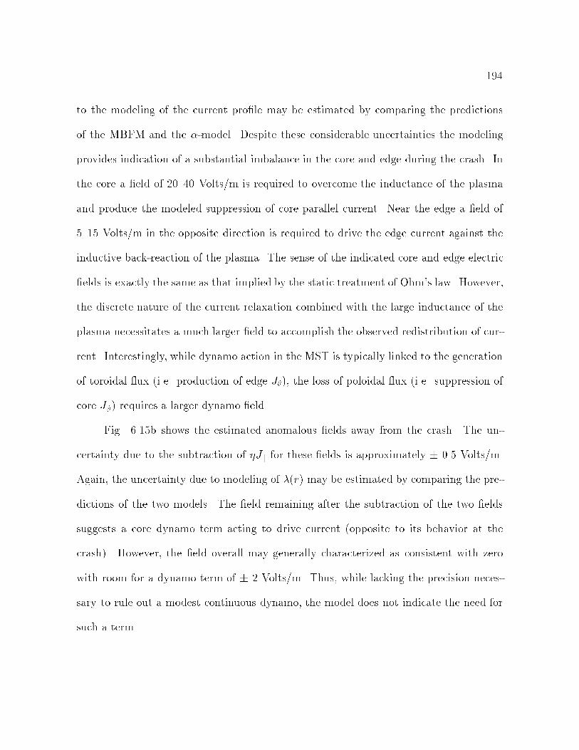
194

to the modeling of the current prole may be estimated by comparing the predictions

of the MBFM and the -model. Despite these considerable uncertainties the modeling

provides indication of a substantial imbalance in the core and edge during the crash. In

the core a eld of 2040 Volts/m is required to overcome the inductance of the plasma

and produce the modeled suppression of core parallel current. Near the edge a eld of

515 Volts/m in the opposite direction is required to drive the edge current against the

inductive back-reaction of the plasma. The sense of the indicated core and edge electric

elds is exactly the same as that implied by the static treatment of Ohm's law. However,

the discrete nature of the current relaxation combined with the large inductance of the

plasma necessitates a much larger eld to accomplish the observed redistribution of cur-

rent. Interestingly, while dynamo action in the MST is typically linked to the generation

of toroidal ux (i.e. production of edge J), the loss of poloidal ux (i.e. suppression of

core J) requires a larger dynamo eld.

Fig. 6.15b shows the estimated anomalous elds away from the crash. The un-

certainty due to the subtraction of Jk for these elds is approximately 0.5 Volts/m.

Again, the uncertainty due to modeling of (r) may be estimated by comparing the pre-

dictions of the two models. The eld remaining after the subtraction of the two elds

suggests a core dynamo term acting to drive current (opposite to its behavior at the

crash). However, the eld overall may generally characterized as consistent with zero

with room for a dynamo term of 2 Volts/m. Thus, while lacking the precision neces-

sary to rule out a modest continuous dynamo, the model does not indicate the need for

such a term.

195

-5 ± 2

1.7

35 ± 10

-30 ± 10

J||

1.7

-1.5 ± 0.5

-1 ± 0.5

0.5 ± 2?

J||

a) b)

c) d)

-2 ± 1

-10 ± 5

10 ± 5

J||

0.5 ± 0.5

-0.5 ± 0.5

0.0 ± 1.0?

J||

Fig. 6.16.| Applied electric eld (voltage source), internally induced electriceld (inductor), dissipated current (resistor), and implied dynamo eld (MSTlogo) shown as four circuit elements. The values shown are in Volts/m with arrowrepresenting their direction relative to the parallel current which moves clockwise.Top circuits show the estimated a) core and b) edge terms during the crash whilebottom circuits show the c) core and d) edge terms away from the crash.

196

Simple Circuit Analogy

We summarize the implications of the mean-eld modeling with the four circuits

shown in Fig. 6.16. During the crash the core is dominated by the internal inductance

of the plasma driving current and the dynamo term suppressing current. In the edge

the situation during the crash is reversed with the inductance of the plasma opposing

the current and the dynamo driving the current. In both cases these terms dominate

the applied and the resistive terms by roughly an order of magnitude. The poloidal

pitch of the magnetic eld at the edge eectively removes the applied eld from the

circuit. Away from the crash in the core the applied eld is roughly balanced by the

inductance of the plasma and the dissipated current with no need for a dynamo term.

Similarly at the edge the inductance of the plasma balances the resistive dissipation of

the poloidal current with no apparent need for a dynamo. Future measurements of the

parallel current prole and plasma resistivity combined with modeling which incorporates

these additional constraints will, almost certainly, change the values assigned to many of

these circuit elements. However, the basic features of these circuits stem directly from the

sudden attening of the parallel current prole. Thus, while numerically approximate,

the modeling described above provides a basic understanding of the dynamic balance of

Ohm's law in the core and edge which we expect to be rened but not reversed by future

measurements.

6.2 Core Dynamo Electric Field

In this section we present the measured dynamo products and provide empirical

estimates of h~v~bi in the interior of MST. These measurements constitute the key novel

results of this thesis. In rough order of importance the measurements demonstrate the

197

existence, illustrate the behavior, and approximate the magnitude of a h~v ~bi dynamo

eld in the interior of MST. The overall behavior of the elds matches many of our

expectations, although careful numerical comparisons with the dynamo elds implied by

the equilibrium modeling proved inconclusive. Achieving such a comparison through a

careful coordination of uctuation measurements and equilibrium modeling await as the

next obvious step in dynamo measurements in MST.

Below we rst present the four dominant h ~v~b;ni and h ~v~b;ni products. These will

be described in a fairly brief manner as most (if not all) of their features derive from

the amplitude, phase, and coherence of the ~v and ~b uctuations, presented previously

in Chapters 4 and 5. We also present the Lundquist number scaling of these products.

Next, we adjust the phase and amplitude of the products to re ect the implied h ~v ~bri and

h ~v ~bri products in the core. The uncertainties of the amplitude adjustment will dominate

the uncertainty in the estimated core dynamo elds. Finally we compare the measured

elds with the predictions of the modeling discussed in x 6.1.

6.2.1 Measured Dynamo Products

Time and frequency behavior of h ~v~b;ni and h ~v~b;ni

The real and imaginary components of the four largest h~v~b;ni products (Fig. 6.17)

are consistent with the amplitude, coherence, and phase of the eld and ow uctuations

presented in Chapters 4 and 5. Like the amplitudes and coherence of the uctuations,

the products peak in time during the sawtooth with cross-power concentrated in fre-

quency from 820 kHz. The relative magnitude of the toroidal and poloidal products

simply re ects the amplitude of the core modes coherent with ~v relative the edge modes

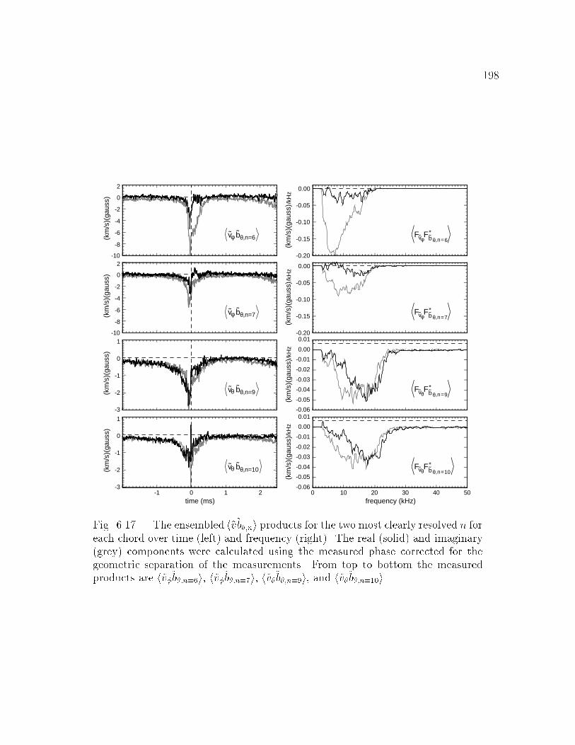
198

-10

-8

-6

-4

-2

0

2

(km

/s)(

gaus

s)

-10

-8

-6

-4

-2

0

2

(km

/s)(

gaus

s)

-3

-2

-1

0

1

(km

/s)(

gaus

s)

-3

-2

-1

0

1

(km

/s)(

gaus

s)

-1 0 1 2time (ms)

0 10 20 30 40 50-0.06

-0.05

-0.04

-0.03

-0.02

-0.01

0.00

0.01

-0.20

-0.15

-0.10

-0.05

0.00

-0.20

-0.15

-0.10

-0.05

0.00

-0.06

-0.05

-0.04

-0.03

-0.02

-0.01

0.00

0.01

(km

/s)(

gaus

s)/k

Hz

(km

/s)(

gaus

s)/k

Hz

(km

/s)(

gaus

s)/k

Hz

(km

/s)(

gaus

s)/k

Hz

frequency (kHz)

vφ bθ,n=6

vφ bθ,n=7

vθ bθ,n=9

vθ bθ,n=10

FvφFbθ,n=6

*

FvφFbθ,n=7

*

FvθFbθ,n=9

*

FvθFbθ,n=10

*

Fig. 6.17.| The ensembled h~v~b;ni products for the two most clearly resolved n foreach chord over time (left) and frequency (right). The real (solid) and imaginary(grey) components were calculated using the measured phase corrected for thegeometric separation of the measurements. From top to bottom the measuredproducts are h~v~b;n=6i, h~v~b;n=7i, h~v~b;n=9i, and h~v~b;n=10i.

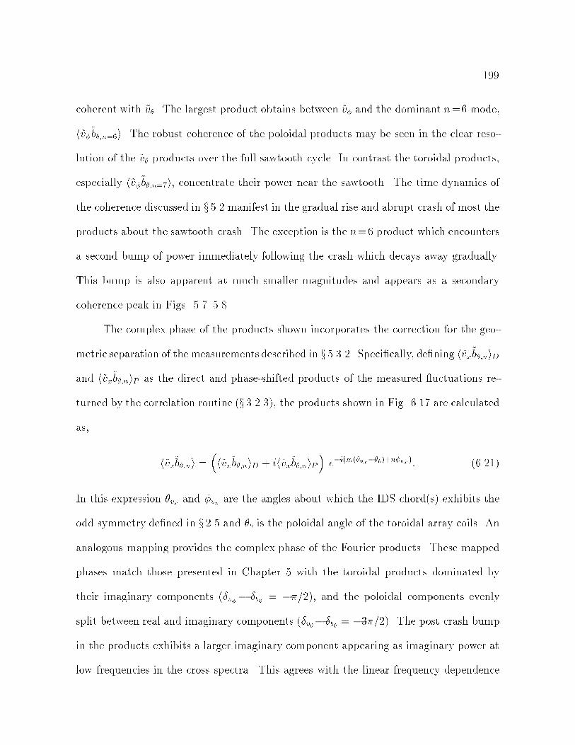
199

coherent with ~v. The largest product obtains between ~v and the dominant n=6 mode,

h~v~b;n=6i. The robust coherence of the poloidal products may be seen in the clear reso-

lution of the ~v products over the full sawtooth cycle. In contrast the toroidal products,

especially h~v~b;n=7i, concentrate their power near the sawtooth. The time dynamics of

the coherence discussed in x 5.2 manifest in the gradual rise and abrupt crash of most the

products about the sawtooth crash. The exception is the n=6 product which encounters

a second bump of power immediately following the crash which decays away gradually.

This bump is also apparent at much smaller magnitudes and appears as a secondary

coherence peak in Figs. 5.75.8.

The complex phase of the products shown incorporates the correction for the geo-

metric separation of the measurements described in x 5.3.2. Specically, dening h~vx~b;niDand h~vx~b;niP as the direct and phase-shifted products of the measured uctuations re-

turned by the correlation routine (x 3.2.3), the products shown in Fig. 6.17 are calculated

as,

h~vx~b;ni =h~vx~b;niD + ih~vx~b;niP

ei(m(vxb)+nvx ): (6.21)

In this expression vx and vx are the angles about which the IDS chord(s) exhibits the

odd symmetry dened in x 2.5 and b is the poloidal angle of the toroidal array coils. An

analogous mapping provides the complex phase of the Fourier products. These mapped

phases match those presented in Chapter 5 with the toroidal products dominated by

their imaginary components (v b = =2), and the poloidal components evenly

split between real and imaginary components (v b = 3=2). The post crash bump

in the products exhibits a larger imaginary component appearing as imaginary power at

low frequencies in the cross spectra. This agrees with the linear frequency dependence

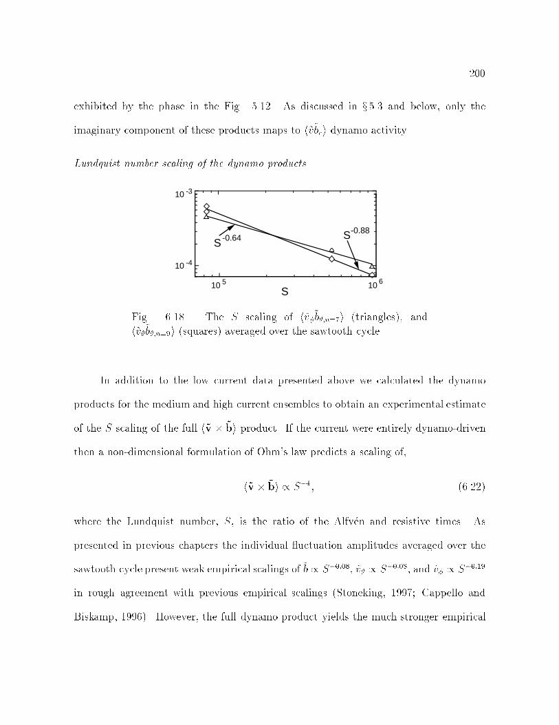
200

exhibited by the phase in the Fig. 5.12. As discussed in x 5.3 and below, only the

imaginary component of these products maps to h~v~bri dynamo activity.

Lundquist number scaling of the dynamo products

10 5 10 6

S

10 -3

10 -4

S-0.88

S-0.64

Fig. 6.18.| The S scaling of h~v~b;n=7i (triangles), and

h~v~b;n=9i (squares) averaged over the sawtooth cycle.

In addition to the low current data presented above we calculated the dynamo

products for the medium and high current ensembles to obtain an experimental estimate

of the S scaling of the full h~v ~bi product. If the current were entirely dynamo-driven

then a non-dimensional formulation of Ohm's law predicts a scaling of,

h~v ~bi / S1; (6.22)

where the Lundquist number, S, is the ratio of the Alfven and resistive times. As

presented in previous chapters the individual uctuation amplitudes averaged over the

sawtooth cycle present weak empirical scalings of ~b / S0:08, ~v / S0:08, and ~v / S0:19

in rough agreement with previous empirical scalings (Stoneking, 1997; Cappello and

Biskamp, 1996). However, the full dynamo product yields the much stronger empirical

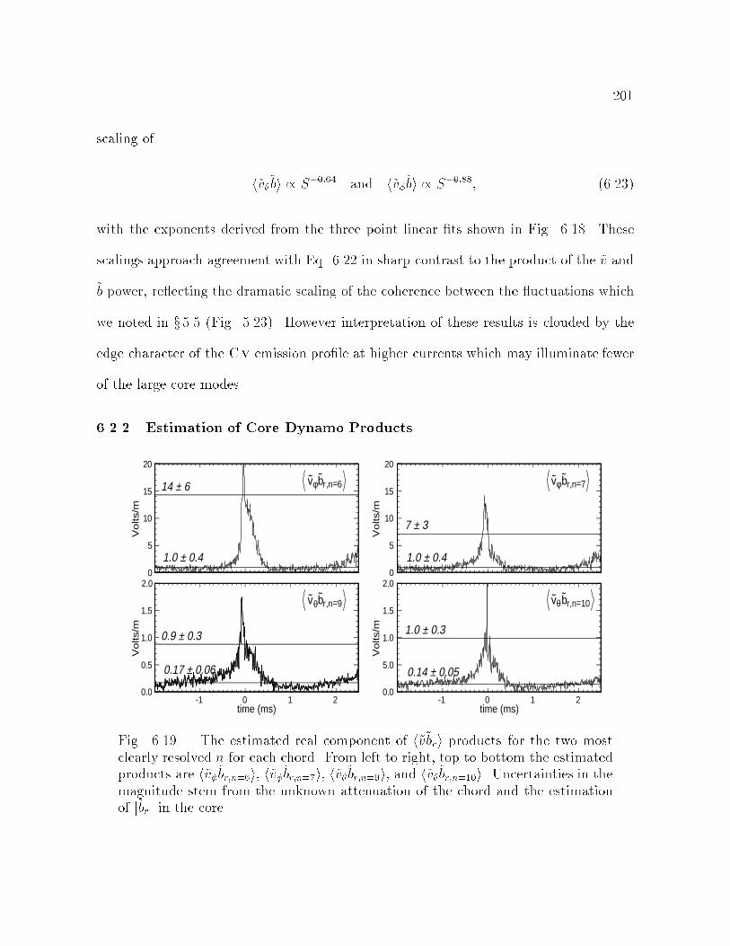
201

scaling of

h~v~bi / S0:64 and h~v~bi / S0:88; (6.23)

with the exponents derived from the three point linear ts shown in Fig. 6.18. These

scalings approach agreement with Eq. 6.22 in sharp contrast to the product of the ~v and

~b power, re ecting the dramatic scaling of the coherence between the uctuations which

we noted in x 5.5 (Fig. 5.23). However interpretation of these results is clouded by the

edge character of the Cv emission prole at higher currents which may illuminate fewer

of the large core modes.

6.2.2 Estimation of Core Dynamo Products

vθbr,n=9

vφbr,n=7vφbr,n=6

vθbr,n=10

-1 0 1 2time (ms)

-1 0 1 2time (ms)

20

15

10

5

02.0

1.5

1.0

0.5

0.0

20

15

10

5

02.0

1.5

1.0

5.0

0.0

1.0 ± 0.4 1.0 ± 0.4

0.17 ± 0.06 0.14 ± 0.05

14 ± 6

7 ± 3

1.0 ± 0.30.9 ± 0.3

Volts/m

Volts/m

Volts/m

Volts/m

Fig. 6.19.| The estimated real component of h~v~bri products for the two mostclearly resolved n for each chord. From left to right, top to bottom the estimatedproducts are h~v~br;n=6i, h~v~br;n=7i, h~v~br;n=9i, and h~v~br;n=10i. Uncertainties in themagnitude stem from the unknown attenuation of the chord and the estimationof j~brj in the core.

202

Direction of Core Dynamo Field

To map the measured h ~v~b;ni and h ~v~b;ni products onto core h ~v ~bri and h ~v ~bri

products we must properly account for the phase shift between ~br in the core and ~b

at the edge. This mapping rotates the negative imaginary component of the measured

products around 90o such that they become positive real components of core h ~v ~bri and

h ~v ~bri products (Fig. 6.19). To interpret these directions we return to the full expansion

of h~v ~bi

h~v ~bi = h ~v ~bri h~vr~bi h ~v ~bri; (6.24)

h~v ~bi = h~vr~bi h ~v ~bri h ~v ~bri; (6.25)

where the h~vr~bi terms are neglected due to the small size and coherence of the measured

radial velocity uctuations (x 5.4). Thus, our positive h ~v ~bri measurement implies a

h~v ~bi at r=a 0:3 0:4 in the + direction. Referring back to our right handed

geometry we see that this corresponds to a current drive such as to drive Jk in the plasma

mid-region and generate B. Thus the h ~v ~bri product is consistent with \dynamo" (as

in not \anti-dynamo") activity in the middle to core region of the plasma. Our positive

h ~v ~bri measurements imply a h~v ~bi at r=a0.60.7 in the direction. This is the

same direction as the applied electric eld and thus should also act to drive parallel

current inside the reversal surface. However, due to the oblique projection of onto the

mean magnetic eld at the edge, very little of this dynamo eld aligns with the edge

parallel current. Conversely, if this measured eld represents the toroidal projection of a

parallel eld, it would imply a substantial h~v ~bik at this radius. Clearly, edge h ~v ~bri

measurements are needed to conrm this. In addition core measurements of h ~v ~bri are

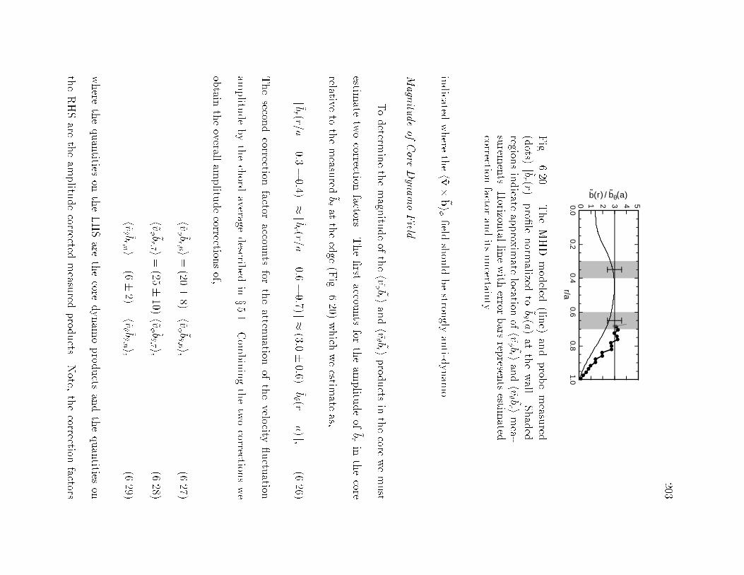
203

0.00.2

0.40.6

0.81.0

543210

r/a

b(r) / bθ(a)Fig.

6.20.|TheMHD

modeled

(line)

andprob

emeasu

red

(dots)j ~b

r (r)jpro

lenorm

alizedto

~b (a

)at

thewall.

Shaded

regionsindicate

approx

imate

locationofh

~v~br i

andh~v~br i

mea-

surem

ents.

Horizon

tallinewith

errorbars

represen

tsestim

atedcorrection

factorandits

uncertain

ty.

indicated

where

theh~v

~bield

should

bestron

glyanti-d

ynam

o.

Magn

itude

ofCore

Dynam

oField

Todeterm

inethemagn

itudeof

theh

~v~br i

andh~v~br i

prod

ucts

inthecore

wemust

estimate

twocorrection

factors.Therst

accounts

fortheam

plitu

deof

~brin

thecore

relativeto

themeasu

red~bat

theedge

(Fig.

6.20)which

weestim

ateas,

j ~br (r=a

=0:3

0:4)jj ~b

r (r=a=0:6

0:7)j(3:0

0:6)j ~b (r

=a)j;

(6.26)

Thesecon

dcorrection

factoraccou

nts

fortheatten

uation

ofthevelocity

uctu

ation

amplitu

debythechord

averagedescrib

edinx5.1.

Com

biningthetwocorrection

swe

obtain

theoverall

amplitu

decorrection

sof,

h~v ~b

r;6 i=(20

8)h~v

~b;6 i;

(6.27)

h~v ~b

r;7 i=(25

10)h~v ~b

;7 i;

(6.28)

h~v ~b

r;n i=(6

2)h~v

~b;n i;

(6.29)

where

thequantities

ontheLHSare

thecore

dynam

oprod

ucts

andthequantities

on

theRHSare

theam

plitu

decorrected

measu

redprod

ucts.

Note,

thecorrection

factors

204

stemming from the attenuation of the toroidal chord is substantial, while the poloidal

chord has a more modest correction of 2 for the attenuation times 3 for the ~b ! ~b

mapping. The errors estimated for these correction factors dominate all other errors

(i.e. instrumental, statistical) in our calculation of the magnitude of the core dynamo

products

We resolve dynamo eld with both chords at and away from the sawtooth crash.

Fig. 6.19 shows the real part of the core dynamo products following the above cor-

rections of phase and amplitude. We obtain dynamo elds from the toroidal velocity

measurements which peak during the crash with amplitudes of,

h~v~br;6i =14 6 Volts/m; at (r=a = 0:3 0:4; jtj 0:05); (6.30)

h~v~br;7i =17 3 Volts/m; at (r=a = 0:3 0:4; jtj 0:05); (6.31)

where the values re ect an average over a 0.1 ms window centered about the sawtooth

and the uncertainties re ect the uncertainties in the mapping. These greatly exceed the

poloidal velocity products during the crash which similarly yield amplitudes of,

h~v~br;9i =0:9 0:3 Volts/m; at (r=a = 0:6 0:7; jtj 0:05); (6.32)

h~v~br;10i =1:0 0:3 Volts/m; at (r=a = 0:6 0:7; jtj 0:05): (6.33)

Away from the crash the average values were calculated by excluding a 1 ms window

about the sawtooth. These yielded values which were typically smaller by a factor of 10,

h~v~br;6i = 1:0 0:4 Volts/m; at (r=a = 0:3 0:4; jtj 0:5); (6.34)

h~v~br;7i = 1:0 0:4 Volts/m; at (r=a = 0:3 0:4; jtj 0:5); (6.35)

h~v~br;9i =0:17 0:06 Volts/m; at (r=a = 0:6 0:7; jtj 0:5); (6.36)

h~v~br;10i =0:14 0:06 Volts/m; at (r=a = 0:6 0:7; jtj 0:5): (6.37)

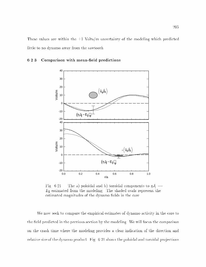
205

These values are within the 1 Volts/m uncertainty of the modeling which predicted

little to no dynamo away from the sawtooth.

6.2.3 Comparison with mean-eld predictions

0.0 0.2 0.4 0.6 0.8 1.0r/a

Vol

ts/m

30

20

10

0

-10

-20

40

vθ br

ηJ|| −E||( )φ

ηJ|| −E||( )θ

Vol

ts/m

30

20

10

0

-10

-20

40

vφbr

-

Fig. 6.21.| The a) poloidal and b) toroidal components to Jk Ek estimated from the modeling. The shaded ovals represent theestimated magnitudes of the dynamo elds in the core.

We now seek to compare the empirical estimates of dynamo activity in the core to

the eld predicted in the previous section by the modeling. We will focus the comparison

on the crash time where the modeling provides a clear indication of the direction and

relative size of the dynamo product. Fig. 6.21 shows the poloidal and toroidal projections

206

of the parallel dynamo elds predicted by both models during the sawtooth crash. For

the h ~v ~bri measurements we measure a dynamo eld of 10 Volts/m in the direction

which corresponds to a parallel current drive, or dynamo term. The modeling predicts a

eld with a similar magnitude but in the opposite direction in the core region coincident

with the h ~v ~bri measurement. The direction of the eld in the core re ects the strong

\anti-dynamo" term necessary to suppress the core parallel current. which is primarily

in the direction with a considerably smaller projection in the direction. Thus it

may be that meausurement of h ~v ~bri in the core would yield a strongly \anti-dynamo"

E which produced a net Ek in the proper direction. This would indicate the existance of

a substantial h~v ~bi? in the core which our modeling would not predict. Thus, with the

present modeling the empirically estimated h~v ~bi eld is approximately the right size

with the \wrong" sign. However, the total sign of Ek in the core is not determined. The

small projected h ~v ~bri term is also directed to drive current, in the edge where the modeled

eld also drives current. Unfortunately, the projection of the estimated JkEk in the

direction is very small in the edge region due to the poloidal pitch of the eld lines. Thus

we have a small measured eld in agreement with a small projected eld. Clearly, h ~v ~bri

measurements in the core are indicated where the enormous \anti-dynamo" electric eld

is projected along with h ~v ~bri measurements in the edge to measure the clear \dynamo"

electric eld.

References

Cappello, S. and D. Biskamp (1996). Reconnection processes and scaling laws in ReversedField Pinch MHD. Nuclear Fusion 36(5), 571581.

Spitzer, Jr., L. (1962). Physics of Fully Ionized Gases. New York: Interscience Publishers.

207

Stoneking, M. R., J. T. Chapman, D. J. Den Hartog, S. C. Prager, and J. S. Sar (1997).Experimental scaling of uctuations and connement with Lundquist number inthe RFP. Phys. Plasmas 5(4), 10041014.

208

7

Summary and Conclusions

Developments in experimental technique

The results presented in this thesis were obtained via several key developments in

measurement, analysis, and modeling techniques. The most important new experimental

technique was the formal development of the Ion Dynamics Spectrometer to measure

the dominant long wavelength velocity uctuations in MST. This involved expressing

the complete eect of averaging velocity over toroidal and polodal chords through ra-

dial mode dependent instrument functions. Application of these instrument functions

allowed the uctuation phase and amplitude measured by the spectrometer to be prop-

erly adjusted to re ect the local phase and amplitude of uctuations in the plasma. The

subsequent measurement and analysis of ~v and ~v demonstrated this capacity along with

an impressive instrumental ability to resolve rapid and tiny shifts in the centroid of the

measured Cv emission prole.

The development of standardized sawtooth ensemble techniques enabled the reso-

lution of the distinctive time and frequency characteristics of noisy velocity uctuation

signals. Novel aspects of this analysis include the incorporation of wavelet analysis and

209

careful selection and screening of sawtooth events to create a tightly constrained ensem-

ble. The former allowed for the identication of unique uctuation features in frequency

and time and for the observation of the time dependent velocity and magnetic uctuation

spectra and cross-spectra. The latter allowed for the careful and consistent description

of narrow regimes in operational parameter space with minimal contamination from out-

lying events.

The analysis of the h ~v~b;ni and h ~v~b;ni products demonstrated the power of corre-

lating \single-point" measurements with the dominant Fourier magnetic modes. These

modes essentially provide the spatial Fourier basis functions in the reference frame of the

plasma converted to a time varying signal in the lab frame. Through the time correlation

of a signal with the individual modes we may eectively perform the spatial Fourier de-

composition in the rotating reference frame of the plasma. In this study the correlation

allowed us to determine the dominant toroidal wavenumbers of the chord-averaged ~v and

~v and to extract the phase of each wavenumber contribution relative to the magnetic

modes.

Summary of experimental results

The measurement of a nite dynamo electric eld in the core of the plasma consti-

tutes the key experimental result of this thesis. Specically, we found that the ensembled

nonlinear product of h ~v ~bri yields a dynamo electric eld which peaks during the saw-

tooth crash to approximately 10 Volts/m in the poloidal direction consistent with the

generation of toroidal ux at r=a 0:30.4. The h ~v ~bri produces a peak toroidal electric

eld of approximately 1 Volt/m which is aligned in the toroidal direction with the exter-

nally applied electric eld at r=a 0:60.7. Away from the crash both products yield

210

small but nite products in the same direction as the peak eld but with one tenth the

amplitude.

The measurement of ion velocity uctuations of several km/s in the core and edge

regions of the MST constitutes the second important contribution of this thesis. These

uctuations peak with the magnetic uctuations during the crash and exhibit a com-

paratively small amplitude away from the crash. Fluctuation power averaged over the

sawtooth cycle for ~v and ~v agrees with our expectation from MHD simulation with

an amplitude of roughly 5% the Alfven velocity. Analysis of the wavenumber spectra of

the chord averaged ~v and ~v measurements indicates that the velocity uctuation level

from a particular mode drops o rapidly away from the rational surface of the mode.

This contrasts with the magnetic uctuations which extend over the full plasma radius.

This eect is present but less pronounced in the MHD simulation which predict global

magnetic modes extending over the full radius and velocity uctuations for the dominant

modes extend over roughly 70% of the plasma radius. Radial velocity uctuations were

somewhat smaller than the other two components and exhibited little coherence with the

core magnetic modes. Thus, the measured contribution of ~vr to the total h~v~bi is small

relative to the h ~v ~bri and h ~v ~bri terms.

Equilibrium modeling of the mean elds indicates that the rapid relaxation of the

current prole during the sawtooth crash induces electric elds which dominate both

the parallel electric eld dissipated by Jk and the toroidal electric eld applied by the

transformer. To balance Ohm's law these induced elds imply a dynamo term which

opposes current in the core and drives current at the edge with a peak magnitude of

2040 Volts/m. The sense of this implied dynamo term agrees with the conclusions of a

static Ohm's law analysis while the magnitude is some ten times larger. The magnitudes

211

inferred from the modeling agree with the dynamo elds observed in the experiment

however the direction of the dynamo E;k predicted in the core contradicts the measured

sign of the h ~v ~bri product.

Both velocity uctuation and magnetic uctuation levels scale little with Lundquist

number. A weak scaling emerges when the uctuations are averaged over the sawtooth

scale due to the decreasing duty cycle of the uctuations at high Lundquist regimes.

However, the full non-linear dynamo product scales nearly as S1 due to decreasing

coherence of the measured uctuations at high currents. The scaling of the measured

dynamo products agrees with the a non-dimensional Ohm's law.

Concluding comments and suggestions for future work

While the current measurements provide clear evidence of dynamo activity in the

core of MST, interpretation of the measured eld direction is ambiguous. In the core

where we expect strong \anti-dynamo" elds acting to suppress core toroidal current we

measure a core poloidal component of the dynamo electric eld directed to drive parallel

current and generate toroidal ux. One explanation for this discrepancy would be a h ~v ~bri

term in the core which produces a strong \anti-dynamo" toroidal electric eld cancelling

out the weak parallel projection of the measured \dynamo" E. One might conjecture

that if h ~v ~bri maintained the same sign over the full plasma radius, it would dominated

near the edge where the magnetic eld is primarily poloidal and the dynamo eld should

drive current and it would be dominated in the core by a possible \anti-dynamo", E

term.

Two measurements would clarify this important issue. First, h ~v ~bri should be mea-

sured near the core to conrm the presence of a large, unambiguously \anti-dynamo"

212

toroidal electric eld. This should be combined with the measured h ~v ~bri term to esti-

mate the total parallel eld and conrm that it suppresses core current. This measure-

ment could be carried out immediately, with current hardware and port access. Second,

h ~v ~bri should be measured near the edge to conrm the presence of a large, unambigu-

ously \dynamo" poloidal electric eld. This measurement is currently underway with an

optical probe extension to the IDS.

Future eorts should be directed toward constraining the numerical balance of par-

allel Ohm's law in MST. First, this involves improvements in modeling of the mean eld

terms to Ohm's law. Integration of new Jk(r) measurements with a toroidal equilibrium

solver should provide greatly improved estimates of the mean eld dynamics while im-

proved measurements of Te(r) and Zeff (r) will provide better estimates of the plasma

resistivity. We expect the improved modeling to agree with features of the modeling

described in this thesis which stem from the general attening of (r). However, greater

numerical accuracy is needed especially in the resolution of a mean-eld Ohm's law im-

balance (or balance) away from the sawtooth crash.

Second, numerical balance of parallel Ohm's law will involve continued measure-

ments of h~v ~bi in the plasma interior. In addition to the two measurements recom-

mended above long-term pursuits include local h~v ~bi measurements performed using

active spectroscopy (CHERS) providing, in principle, for the local measurement of h~v~bi

over the full plasma radius. Coordination of Langmuir probe measurements like those

performed by Ji and novel edge ~v measurements with the IDS probe will further de-

scribe edge dynamo activity. While the measurements presented in this work conrm

the presence of an MHD dynamo electric eld, future eorts should complete the task of

balancing Ohm's law balance over the interior of the reversed-eld pinch.

213

A

Toroidal Calculation of Magnetic Boundary

The results obtained x 4.2.2 for the boundary conditions with a cylindrical analysis hold

with only slight modications in an analogous toroidal analysis. This primarily involves

the retention of terms involving the poloidal derivative of b and b and neoclassical terms

O( aR). Expanding the toroidal analog to Eq. 4.9 we have,

0 ~jr(a; ) = rr r~b

r=a

= rr r~brrr +r(r~b)r+r(R~b)r

=

@(R~b)

@ @(r~b)

@

!(rr) rr

= i nbRei(m+n+!t+b )imb

aei(m+n+!t+b )

+ba

1

b

@b@

a

Rsin()

ei(m+n!t+b )

= 0: (A.1)

The toroidal correction introduces a third term to the RHS of Eq. A.1 which is out of

phase with the two cylindrical terms. This term introduces a small phase shift between

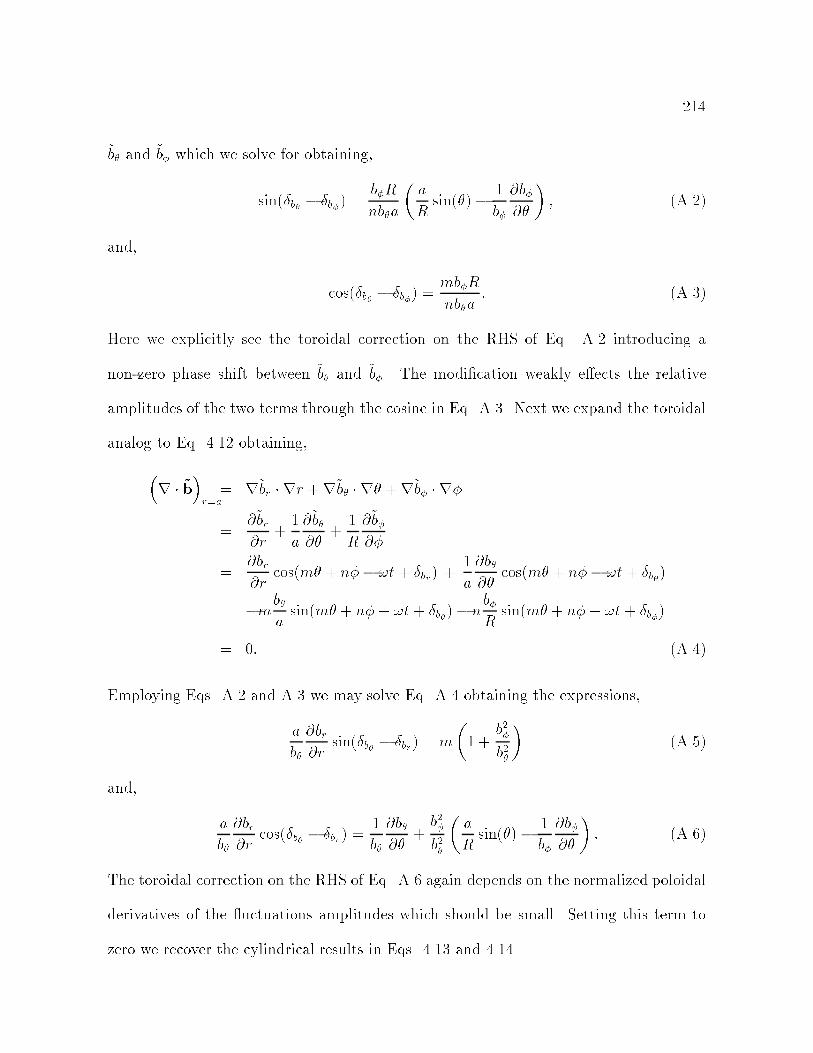
214

~b and ~b which we solve for obtaining,

sin(b b) =bR

nba

a

Rsin() 1

b

@b@

; (A.2)

and,

cos(b b) =mbR

nba: (A.3)

Here we explicitly see the toroidal correction on the RHS of Eq. A.2 introducing a

non-zero phase shift between ~b and ~b. The modication weakly eects the relative

amplitudes of the two terms through the cosine in Eq. A.3. Next we expand the toroidal

analog to Eq. 4.12 obtaining,

r ~b

r=a

= r~br rr +r~b r +r~b r

=@~br@r

+1

a

@~b@

+1

R

@~b@

=@br@r

cos(m + n !t+ br) +1

a

@b@

cos(m + n !t+ b)

mbasin(m + n+ !t+ b) n

bRsin(m + n+ !t+ b)

= 0: (A.4)

Employing Eqs. A.2 and A.3 we may solve Eq. A.4 obtaining the expressions,

a

b

@br@r

sin(b br) = m

1 +

b2b2

(A.5)

and,

a

b

@br@r

cos(b br) =1

b

@b@

+b2b2

a

Rsin() 1

b

@b@

: (A.6)

The toroidal correction on the RHS of Eq. A.6 again depends on the normalized poloidal

derivatives of the uctuations amplitudes which should be small. Setting this term to

zero we recover the cylindrical results in Eqs. 4.13 and 4.14.

215

B

Computer Code Listings

This appendix contains a partial listing of the code employed for the calculations de-

scribed in this thesis. Not included in this listing are a large number of supportine subrou-

tines which may be found in the directory [jchaman.idl]or in the [.subroutine] subdi-

rectory appropriate to the main routine. The sawtooth selection routines sawlist.pro,

sawtype.pro, and sawselect.pro were also omitted as most of their large size gov-

erns a freindly user interface. In their place truncated sawtooth listings are included

which demonstrate the creation of a sawtooth ensemble. Much of this code remains in

widespread public use and will hopefully continue to evolve with the needs of its users.

B.1 IDS Data Processing

These routines govern the conversion of raw spectrometer data into impurity tem-

peratures and velocities. A overview of these algorithms may be found in x 2.3.

B.1.1 IDS Fitting Engine

The noninteractive routine fit.com serves as the front end for the IDS t engine.

The user denes the variables in this le and submits the job to a VMS batch queue.

216

The batch routien then denes the necessary variables, compiles the subroutines, and

calls the main IDS t engine. These routines are described in x 2.3.

$ set def [jchapman.public.flow]

$ idl

;;;;==================================================================

;;;; FIT.COM

;;;; Ion Dynamics Spectrometer - Gaussian Fit Engine (Batch Startup File)

;;;; J. T. Chapman University of Wisconsin - Madison May 27, 1997

;;;;==================================================================

;;;-------------------------------------------------------------------

;;; The variable SHOTLIST MUST BE DEFINED FOR FIT.PRO TO WORK. The shotlist

;;; is an ascii file located in the users directory which contains the shot

;;; numbers, dates, starting times, and ending times for all the shots to be

;;; processed in the batch job.

;;; To make a shot list enter idlv2 and run the main level routine

;;; MAKELIST.PRO. This will prompt you for everything and write a properly

;;; formatted shot file to the directory you specify.

;;; If you desire to use your own routines to write a shot file it must be

;;; formatted as: format='(2x,i3,2x,a11,2x,i5,2x,i5)',shot,date,t1,t2.

;;; The last shot in the shotlist file must be 0. This signals the routine

;;; that the shotlist has terminated. The routine will pay attention to no

;;; shots listed beyond the shot labeled 0.

;;; Negative shot numbers signal fit.pro to calculate a new x_lam

;;; using the data from that shot. If all shots are positive and x_lam is

;;; left undefined the first shot is used for the calibration. If

;;; x_lam is already defined that value will be used unless a

;;; negative shot number is encountered.

shotlist = "[myname.mydirectory]myshotlist.lsa"

;;;-------------------------------------------------------------------

;;; The variable fit_freq sets the frequency of the signal input to the

;;; non-linear fit routine. This should set above 10.0 only if you have

;;; some serious time on your hands or are running on something other than

217

;;; CHAOS. Below 1.0 the routine time is dominated by MDS access time and

;;; further reductions do not save much time. The routine defaults to a

;;; fit_freq=10.0 kHz if the variable is undefined.

fit_freq = 10.0

;;;-------------------------------------------------------------------

;;; This flag sets whether the fit engine plots moments of the fits as the

;;; shots are processed. This flag should not be raised in

;;; batch mode (the plots have nowhere to go). Plot fits defaults to 0.

plot_fits=0

;;; Term type sets the terminal type for the plot routine to use.

;;; If undefined it defaults to a tektronics terminal.

term_type='tek'

;;;-------------------------------------------------------------------

;;; This flag indicates the orientation of the channels to port positions.

;;; The standard orientation (1-16)@138 and (17-32)@222 correspond to a

;;; port_pos=1, the opposite to port_pos=-1. With these settings

;;; a positive flow corresponds to a flow in the direction of increasing

;;; toroidal angle (i.e. opposite the usual direction of core flow).

port_pos=1

;;;-------------------------------------------------------------------

;;; This variable corresponds to the voltage on the PMT's for the run.

;;; It defaults to 1100 V. If set to a negative value the value is

;;; set per shot by reading the thumbwheel #316.

pmt_voltage=1100

;;;-------------------------------------------------------------------

;;; These variables contain all the necessary information about the impurity

;;; emmision. If none of these are set the routine defaults to the settings

;;; for CV. If just the lam_0 variable is set the routine will set the cor-

;;; responding order, m_ion, and imp_ion. If a non-standard lam_0 is used

;;; all variables must be defined.

lam_0 = 2270.9 & order = 5 & m_ion = 12.011 & imp_ion = "CV"

218

; lam_0 = 2296.9 & order = 5 & m_ion = 12.011 & imp_ion = "CIII"

; lam_0 = 2781.0 & order = 4 & m_ion = 15.999 & imp_ion = "OV"

; lam_0 = 2821.7 & order = 4 & m_ion = 10.811 & imp_ion = "BIV"

; lam_0 = 4861.3 & order = 3 & m_ion = 1.008 & imp_ion = "HI"

; lam_0 = 3203.0 & order = 4 & m_ion = 4.003 & imp_ion = "HeII"

; lam_0 = 4685.7 & order = 2 & m_ion = 4.003 & imp_ion = "HeII"

;;;-------------------------------------------------------------------

;;; This variable is non-zero if the user employs only 16 channels of the

;;; IDS array. NOTE: x_lam must be pre-calibrated and defined above to

;;; use this option. The default is one_side=0.

one_side = 0 ; Channels 1-32 (default)

; one_side = 1 ; Channels 1-16

; one_side = 2 ; Channels 17-32

;;;-------------------------------------------------------------------

;;; Here I compile all necessary subroutines

.run [jchapman.idl]thinn

.run [jchapman.idl]vtt

.run [jchapman.idl]defined

.run [jchapman.public.flow.subroutines]chanmap

.run [jchapman.public.flow.subroutines]filecode

.run [jchapman.public.flow.subroutines]gausfit

.run [jchapman.public.flow.subroutines]fit_plot

;;; And now I startup the main routine

.run [jchapman.public.flow]fit

;;;;==================================================================

The Gaussian t engine governs the conversion of raw IDS data into the moments of

Gaussian proles. This time consuming task should be submitted using fit.com to a

queue for overnight processing.

;;;;==================================================================

;;;; FIT.PRO

;;;; Ion Dynamics Spectrometer - Gaussian Fit Engine

;;;; This routine is the primary engine for the conversion of raw

219

;;;; spectrometer data into profiles of Gaussian fit parameters.

;;;; The program reads data from an XDR file or an MDS data base

;;;; transparent to the engine. The data is normalized and baselined

;;;; using current normalization parameters and fit using a standard

;;;; non-linear fit routine. The moments of the gaussian fits are then

;;;; written to XDR files on juno for dropping to the MDS data base.

;;;; Version 1.0 (WindowsNT version)

;;;; J. T. Chapman University of Wisconsin - Madison June 15, 1995

;;;; Version 2.0 (public and alpha versions non-interactive)

;;;; J. T. Chapman University of Wisconsin - Madison May 21, 1997

;;;;==================================================================

;;;-------------------------------------------------------------------

;;; Setup of routine for data fitting

;; greeting for log file

print,format='(80("="))'

print, " "

print, " Ion Dynamics Spectrometer - Gaussian Fit Engine"

print, " J. T. Chapman; University of Wisconsin - Madison; May 21, 1997"

print, " "

print,format='(80("-"))'

;; fit routine settings and parameters

!quiet=1 ;...suppressing compile messages

;...sampling frequency

if (not defined(fit_freq)) then fit_freq=10.0

bin_size=fix(1000.0/fit_freq+0.5)

;...plotting parameters

if (not defined(plot_fits)) then plot_fits=0

if (not defined(term_type)) then term_type='tek'

set_plot,term_type

;; shot file definition, check, and report

;...no shot file defined

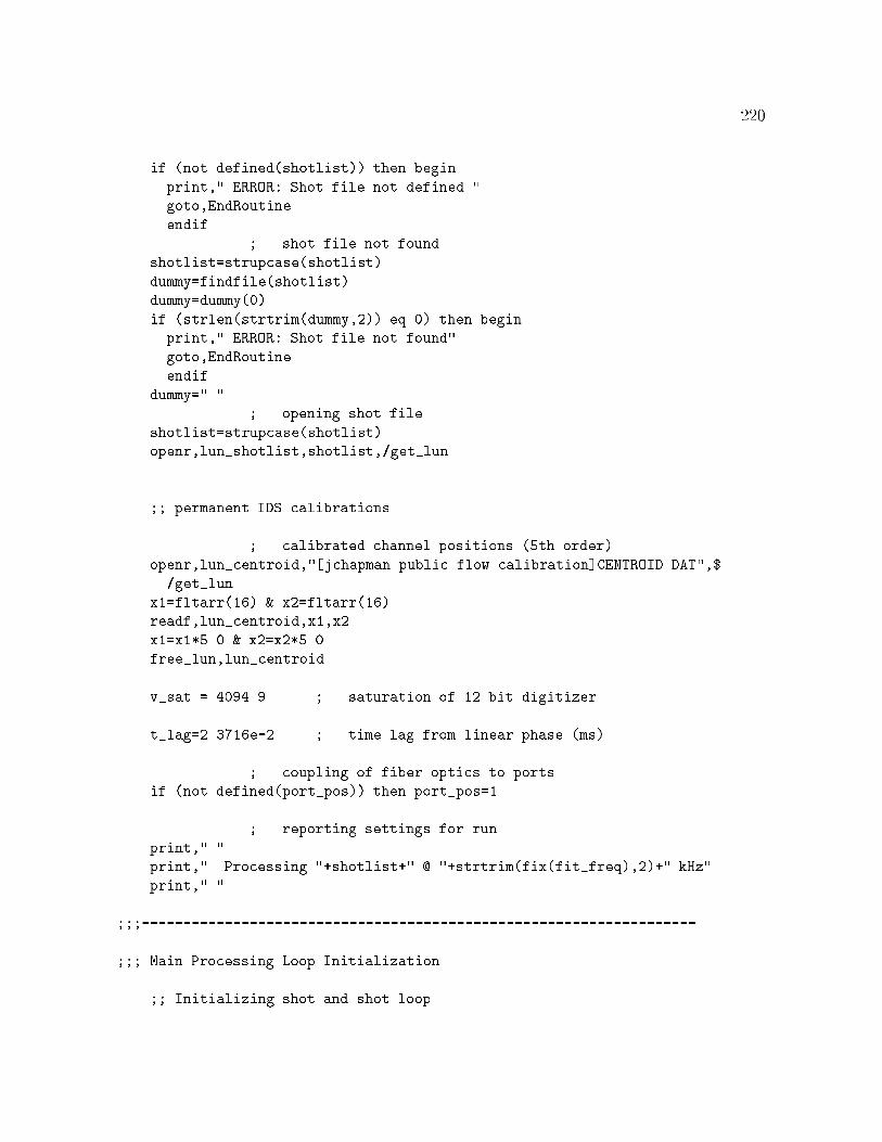
220

if (not defined(shotlist)) then begin

print," ERROR: Shot file not defined."

goto,EndRoutine

endif

;...shot file not found

shotlist=strupcase(shotlist)

dummy=findfile(shotlist)

dummy=dummy(0)

if (strlen(strtrim(dummy,2)) eq 0) then begin

print," ERROR: Shot file not found"

goto,EndRoutine

endif

dummy=" "

;...opening shot file

shotlist=strupcase(shotlist)

openr,lun_shotlist,shotlist,/get_lun

;; permanent IDS calibrations

;...calibrated channel positions (5th order)

openr,lun_centroid,"[jchapman.public.flow.calibration]CENTROID.DAT",$

/get_lun

x1=fltarr(16) & x2=fltarr(16)

readf,lun_centroid,x1,x2

x1=x1*5.0 & x2=x2*5.0

free_lun,lun_centroid

v_sat = 4094.9 ;...saturation of 12 bit digitizer

t_lag=2.3716e-2 ;...time lag from linear phase (ms)

;...coupling of fiber optics to ports

if (not defined(port_pos)) then port_pos=1

;...reporting settings for run

print," "

print," Processing "+shotlist+" @ "+strtrim(fix(fit_freq),2)+" kHz"

print," "

;;;-------------------------------------------------------------------

;;; Main Processing Loop Initialization

;; Initializing shot and shot loop

221

;...initializing shot variables

shot=0 & date='today' & t1=0 & t2=0

;...reading in first shot

readf,lun_shotlist,format='(2x,i3,2x,a11,2x,i5,2x,i5)',shot,date,t1,t2

;...loop is terminated at shot=0

while (shot ne 0) do begin

;...setting up MDS data base for shot

set_db,'mst$data'

dummy=set_shot(abs(shot))

dummy=set_date(date)

;...determining how to handle x_lam calibration

if ((not defined(x_lam)) or (shot lt 0)) then $

calculate_zero_point = 1 $

else $

calculate_zero_point = 0

;; IDS PMT normalization

;...IDS PMT voltage (default 1100 V)

if (not defined(pmt_voltage)) then pmt_voltage=1100

;...get setting from thumbwheel if undefined

if (pmt_voltage lt 0) then pmt_voltage=(-1)*thumbi(316)

;...set to nearest of 900,1000, or 1100 V

pmt_voltage_1 = ((( long(abs(pmt_voltage)/100.+0.5)*100 )>900)<1100)

;opening appropriate file

case pmt_voltage_1 of

900: openr,lun_norm,$

"[JCHAPMAN.PUBLIC.FLOW.CALIBRATION]NORM0900.DAT",/get_lun

1000: openr,lun_norm,$

"[JCHAPMAN.PUBLIC.FLOW.CALIBRATION]NORM1000.DAT",/get_lun

1100: openr,lun_norm,$

"[JCHAPMAN.PUBLIC.FLOW.CALIBRATION]NORM1100.DAT",/get_lun

endcase

norm = fltarr(32) ;...initialize normalization array

readf,lun_norm,norm ;...read in normalizations

free_lun,lun_norm ;...close up normalization file

222

;; Obtaining the impurity emmission information

;...assume CV emmission if not defined

if (not defined(lam_0)) then lam_0=2270.9

;...read in lam_0 from thumbwheels

if (lam_0 lt 0) then lam_0=(-1)*thumbi(310)

;...obtaining ion information

case (float(long(abs(lam_0)*10+0.5))/10.) of

2270.9: begin & order = 5 & m_ion = 12.011 & imp_ion = "CV" & end

2296.9: begin & order = 5 & m_ion = 12.011 & imp_ion = "CIII" & end

2781.0: begin & order = 4 & m_ion = 15.999 & imp_ion = "OV" & end

2821.7: begin & order = 4 & m_ion = 10.811 & imp_ion = "BIV" & end

4861.3: begin & order = 3 & m_ion = 1.008 & imp_ion = "HI" & end

3203.0: begin & order = 4 & m_ion = 4.003 & imp_ion = "HeII" & end

4685.7: begin & order = 2 & m_ion = 4.003 & imp_ion = "HeII" & end

else: if (not (defined(order)*defined(m_ion)) ) then begin

print, " ERROR: Unknown impurity wavelength."

goto,JumpShot

endif

endcase

if (not (defined(one_side))) then one_side=0

if ((one_side ne 0) and calculate_zero_point) then begin

print," ERROR: Unable to calibrate x_lam with only one side."

stop

endif

;...reporting shot settings

if (calculate_zero_point) then $

print," "+date+" #"+strtrim(abs(shot),2)+" ("+strtrim(t1,2)+"-"+$

strtrim(t2,2)+"): "+imp_ion+" ("+strtrim(fix(lam_0+0.5),2)+$

" A) X "+strtrim(order,2)+", PMT's @"+strtrim(pmt_voltage,2)+$

" (x_lam calibrated)." $

else $

print," "+date+" #"+strtrim(abs(shot),2)+" ("+strtrim(t1,2)+"-"+$

strtrim(t2,2)+"): "+imp_ion+" ("+strtrim(fix(lam_0+0.5),2)+$

" A) X "+strtrim(order,2)+", PMT's @"+strtrim(pmt_voltage,2)+"."

223

;; Setting Boundaries and Sigmas for fit routine:

;...boundaries from reasonable physical values

bound = $

[[ 0.0, $ ; fit0 > 0

-(lam_0*1.0e+2)/2.998e+5+2.0, $ ; velocity>-100 km/s

0.0 ], $ ; temperature > 0

[(2^12)*1.5, $ ; fit0<1.5*(12 bits)

(lam_0*1.0e+2)/2.998e+5+2.0, $ ; velocity<100 km/s

sqrt(3.0e3/(931.4812e+6*m_ion))*lam_0 ]] ; temperature<3 keV

;...perturbation values of initial conditions

sigma = [ 2^3, $ ; three bits

(lam_0*1.0e-1)/2.998e+5, $ ; 100 m/s

sqrt(5e0/(931.4812e+6*m_ion))*lam_0, $ ; 5 eV

0,0 ] ; baseline stays

;;;-------------------------------------------------------------------

;;; Getting index start and stop time and time array

;; Time array from data base

;...reading array

if (one_side le 1) then $

timevf_full = data('a2_a14_vf1_tm')*1000. $

else $

timevf_full = data('a2_a14_vf3_tm')*1000.

;...check that it's there

if (n_elements(timevf_full) le 2) then begin

print," No IDS data found."

goto, JumpShot

endif

;...thinning to proper frequency

timevf_full = thinn(timevf_full,bin_size)

;; Finding indices and truncating data

;...start and stop indices

i_start = long( min( where( timevf_full ge t1 ) ) )

i_stop = long( max( where( timevf_full le t2 ) ) )

224

;...baseline subtraction indices

i_base_1 = 1

i_base_2 = long( max( where( timevf_full le -0.01 ) ) )

;...length of data arrays

nn = i_stop - i_start + 1

;...truncate time array

timevf = temporary( float( timevf_full( i_start : i_stop )) )

timevf_full = 0 ;...clear old array

;;;-------------------------------------------------------------------

;;; Normalizing VFS shot data

vf=fltarr(nn,32) ;...2-D array of raw signal for all channels

start_chan=1 & last_chan=32

case one_side of

1: last_chan=16

2: start_chan=17

else: start_chan=1

endcase

for i=start_chan-1, last_chan-1 do begin

;...read data

vftmp=data(chanmap(i+1))

;...skip channel if signal is missing

if (n_elements(vftmp) le 2) then goto,JumpChan

;...find saturated points

i_v=where(vftmp ge v_sat)

;...no saturation -> simple thinn

if (max(i_v) lt 0) then vftmp = thinn(vftmp,bin_size) $

;...thinn data - excluding saturated points

else begin

;... initialize boolean array

vfbol=fltarr(n_elements(vftmp))+1.0

;...set saturate points to zero

225

vfbol(i_v)=0.0 & vftmp(i_v)=0.0

;...thinn two arrays

vftmp = thinn(vftmp,bin_size) & vfbol = thinn(vfbol,bin_size)

;...some non-saturated points -> normalize data

if (max(vfbol) gt 0) then $

vftmp(where(vfbol gt 0))=vftmp(where(vfbol gt 0))$

/vfbol(where(vfbol gt 0))

;...some fully saturated points

if (min(vfbol) eq 0) then vftmp(where(vfbol eq 0))=0.0

vfbol=0 ;...clear boolean array

endelse

;; Truncating, baselineing, and normalizing data

;...truncate raw data

vf(*,i) = temporary(float(vftmp( i_start:i_stop )))

;...getting valid points

vfbol = where(vf(*,i))

;...subtract off data baseline

if (max(vfbol) ne -1) then $

vf(vfbol,i) = temporary(vf(vfbol,i)-avg(vftmp(i_base_1:i_base_2)))

vf(*,i) = vf(*,i)/norm(i)

JumpChan:

endfor

vftmp=0 ;...clearing data array

;;;-------------------------------------------------------------------

;;; Non-linear Gaussian fit

;; Declaration Gaussian fit arrays

;...0th moment of fitted Gaussian @ 12

amp1 = fltarr(nn) & amp2 = fltarr(nn)

226

;...1st moment of fitted Gaussian @ 12

cnt1 = fltarr(nn) & cnt2 = fltarr(nn)

;...2nd moment of fitted Gaussian @ 12

vrn1 = fltarr(nn) & vrn2 = fltarr(nn)

;...baseline of Gaussian fit

bas1 = fltarr(nn) & bas2 = fltarr(nn)

;...baseline slope of Gaussian fit

slp1 = fltarr(nn) & slp2 = fltarr(nn)

;...Chi-square of non-linear fit @ 12

chi1 = fltarr(nn) & chi2 = fltarr(nn)

;; Comforting user feedback

;; Main fitting loop

for j=0L,nn-1 do begin

if (one_side ne 2) then begin

y = vf(j,0:15) ;...filling y array

x = x1/order ;...filling x array

;...valid points

val = where(y ne 0.0)

;...little/no valid data -> Jump Point

if (max(val) eq -1) then goto, JumpPoint1

if (n_elements(val) le 12) then goto, JumpPoint1

y=y(val) & x=x(val) ;...getting rid of invalid points

;...intitial statistical guess

a = [ max(y), $

total(x*y)/total(y), $

sqrt(total(y*(x-total(x*y)/total(y))^2)/total(y)), $

(y(0)+y(n_elements(y)-1))/2.0, $

0.0 ]

;...purging math error queue

dummy = check_math(0,1)

;...curvefit routine for 1

227

goodfit = gausfit(x, y, a, bound, sigma, chisqr)

;...filling moment arrays

amp1(j) = a(0)*(2*goodfit-1)

cnt1(j) = a(1)*(2*goodfit-1)

vrn1(j) = a(2)*(2*goodfit-1)

bas1(j) = a(3)*(2*goodfit-1)

slp1(j) = a(4)*(2*goodfit-1)

;...updating chi2_1

chi1(j) = sqrt(chisqr>0.0)

endif

JumpPoint1:

if (one_side ne 1) then begin

y = vf(j,16:31) ;...filling y array

x = x2/order ;...filling x array

;...valid points

val = where(y ne 0.0)

;...little/no valid data -> Jump Point

if (max(val) eq -1) then goto, JumpPoint2

if (n_elements(val) le 12) then goto, JumpPoint2

y=y(val) & x=x(val) ;...getting rid of invalid points

;...intitial statistical guess

a = [ max(y), $

total(x*y)/total(y), $

sqrt(total(y*(x-total(x*y)/total(y))^2)/total(y)), $

(y(0)+y(n_elements(y)-1))/2.0, $

0.0 ]

;...purging math error queue

dummy = check_math(0,1)

;...curvefit routine for 1

goodfit = gausfit(x, y, a, bound, sigma, chisqr)

;...filling moment arrays

amp2(j) = a(0)*(2*goodfit-1)

cnt2(j) = a(1)*(2*goodfit-1)

vrn2(j) = a(2)*(2*goodfit-1)

228

bas2(j) = a(3)*(2*goodfit-1)

slp2(j) = a(4)*(2*goodfit-1)

;...updating chi2_2

chi2(j) = sqrt(chisqr>0.0)

endif

JumpPoint2:

endfor ;...end of fitting loop

;; Calculating zero point if necessary

if (calculate_zero_point) then begin

;...points which were well fit and 10-20 ms

val = where( (timevf gt 10.) and (timevf lt 20.) )

;...calculate average mean position

if (max(val) ne -1) then begin

x_lam = avg(cnt1(val)+cnt2(val))/2.0

calculate_zero_point=0

endif

endif

;;;-------------------------------------------------------------------

;;; Output of results

nw=put_data('V.VFS_LAM_0',lam_0,'Angstrom')

nw=put_data('V.VFS_PORT_POS',port_pos,'au')

nw=put_data('V.VFS_X_LAM',x_lam,'Angstrom')

nw=put_data('V.VFS_M_ION',m_ion,'amu')

nw=put_data('V.VFS_TIME',timevf,'ms')

if ( port_pos eq 1 ) then begin

if (one_side ne 2) then begin

nw=put_data('V.VFS_138_FIT0',amp1,'Volts')

nw=put_data('V.VFS_138_FIT1',cnt1,'Angstrom')

nw=put_data('V.VFS_138_FIT2',vrn1,'Angstrom')

nw=put_data('V.VFS_138_CHI2',chi1,'Volts')

endif

if (one_side ne 1) then begin

nw=put_data('V.VFS_222_FIT0',amp2,'Volts')

229

nw=put_data('V.VFS_222_FIT1',cnt2,'Angstrom')

nw=put_data('V.VFS_222_FIT2',vrn2,'Angstrom')

nw=put_data('V.VFS_222_CHI2',chi2,'Volts')

endif

endif $

else begin

if (one_side ne 1) then begin

nw=put_data('V.VFS_138_FIT0',amp2,'Volts')

nw=put_data('V.VFS_138_FIT1',cnt2,'Angstrom')

nw=put_data('V.VFS_138_FIT2',vrn2,'Angstrom')

nw=put_data('V.VFS_138_CHI2',chi2,'Volts')

endif

if (one_side ne 2) then begin

nw=put_data('V.VFS_222_FIT0',amp1,'Volts')

nw=put_data('V.VFS_222_FIT1',cnt1,'Angstrom')

nw=put_data('V.VFS_222_FIT2',vrn1,'Angstrom')

nw=put_data('V.VFS_222_CHI2',chi1,'Volts')

endif

endelse

;; Default plotting routines

if plot_fits then begin ;...plotting data?

if ( port_pos eq 1 ) then $

fit_plot,abs(shot),date,x_lam,timevf,amp1,amp2,cnt1,cnt2,vrn1,vrn2 $

else $

fit_plot,abs(shot),date,x_lam,timevf,amp2,amp1,cnt2,cnt1,vrn2,vrn1

vtt

endif

;;;-------------------------------------------------------------------

;;; Wrap of loops and routine

;; End of processing loop

JumpShot: ;...Jump shot label

;...readin next shot

readf,lun_shotlist,format='(2x,i3,2x,a11,2x,i5,2x,i5)',shot,date,t1,t2

endwhile ;...end of shot loop

230

;; End of routine

free_lun,lun_shotlist

;...saying goodbye

print," "

print,format='(80("-"))'

print," "

print," Goodbye."

print," "

print,format='(80("="))'

EndRoutine: ;...end of program

end

;;;;==================================================================

B.1.2 Nonlinear Fit Routine

The function gaust has been substantially modied from the IDL curvefit.pro routine

to optimize its performance for the t of IDS data. This routine is called by the tting

engine and actually performs the nonlinear convergence of the Gaussian model to the

data.

function gausfit, x, y, a, bound, sigma, chisqr

;==========================================================================

; Header

;==========================================================================

; NAME:

; GAUSFIT

; PURPOSE:

; Non-linear least squares fit to a gaussian. Using Marquadt method.

; CALLING SEQUENCE:

; valid = GAUSFIT(X, Y, A, BOUND, SIGMA, CHISQR)

; INPUTS:

; X: A row vector of independent variables.

231

; Y: A row vector of dependent variable, the same length as x.

; A: A vector, with as many elements as the number of terms, that

; contains the initial estimate for each parameter. If A is

; double precision, calculations are performed in double

; precision otherwise they are performed in single precision.

; BOUND: A two-dimensional vector, containing the upper lower bounds on

; the parameters passed in A. If A falls outside these bounds the

; fit is attempted again with perturbed initial conditions.

; SIGMA: Uncertainty acquainted with each parameter. If the fit diverges

; the initial conditions will be randomly perturbed by an amount

; proportional to sigma.

; OUTPUTS:

; Returns boolean (0,1) of whether fit was valid

; A: A vector of parameters containing fit.

; SIGMA: Uncertainty acquainted with the output parameters.

; CHISQR: The value of chi-squared on exit

; PROCEDURE:

; Modified from "CURFIT", least squares fit to a non-linear

; function, pages 237-239, Bevington, Data Reduction and Error

; Analysis for the Physical Sciences.

; "This method is the Gradient-expansion algorithm which

; combines the best features of the gradient search with

; the method of linearizing the fitting function."

; Iterations are performed until the chi square changes by

; only TOL or until ITMAX iterations have been performed.

; The initial guess of the parameter values should be

; as close to the actual values as possible or the solution

; may not converge.

;=======================================================================

; Initialize Variables

;=======================================================================

FALSE = 0. ; Booleans defined

232

TRUE = 1.

on_error,2 ; return to caller if error

count_flambda_max = 10 ; number of flambda jumps

count_pert_max = 3 ; number of IC perturbations

count_iter_max = 10 ; maximum number of iterations

tol = 1.0e-2 ; convergence tolerance

valid = TRUE ; valid initialized to true

converged = FALSE ; converged is initially false

nterms = 5 ; # of parameters

npoints = n_elements(y) ; # of data points in fit

nfree = npoints-nterms ; degrees of freedom

a_old = a ; saving passed a

diag = lindgen(nterms)*(nterms+1) ; subscripts of diagonal elements

;=======================================================================

; Convergence Iteration

;=======================================================================

; gaussian procedure calculates partial derivatives

z = (x-a(1))/a(2) & z2=z^2

base = a(3)+a(4)*x

yfit = a(0)*EXP(-z2/2.0)

pder = [[yfit/a(0)],[yfit*z/a(2)],[yfit*z2/a(2)],$

[1+fltarr(npoints)],[x]]

yfit = yfit + base

chisq0 = total((y-yfit)^2)/nfree

yfit0 = yfit

count_pert=0

while ( valid and (not converged) ) do begin

count_pert=count_pert+1

flambda = 0.001 ; reset lambda

count_iter=0

while ( valid and (not converged) ) do begin

count_iter=count_iter+1

233

; evaluate alpha and beta matricies.

beta = (y-yfit) # pder

alpha = transpose(pder) # pder

; present chi squared

chisq1 = total((y-yfit)^2)/nfree

; invert modified curvature matrix to find new parameters.

count_flambda=0

repeat begin

count_flambda=count_flambda+1

; find new parameters

alpha_prime = alpha

alpha_prime(diag) = alpha_prime(diag)*(1+flambda)

epsilon = invert(alpha_prime)

b = a + (epsilon # transpose(beta))

; calculate new fit

z = (x-b(1))/b(2) & z2=z^2

base = b(3)+b(4)*x

yfit = b(0)*EXP(-z2/2.0)

pder = [[yfit/b(0)],[yfit*z/b(2)],[yfit*z2/b(2)],$

[1+fltarr(npoints)],[x]]

yfit = yfit + base

chisqr = total((y-yfit)^2)/nfree ; calculate new chisqr

flambda = flambda*10. ; assume fit got worse

; has the flambda max count been exceeded

if (count_flambda gt count_flambda_max) then valid=FALSE

endrep until ((not valid) or $

(chisqr lt chisq1))

flambda=flambda/100. ; decreasing flambda by 100/10

; check to see if fit is diverging

if ( min(b gt bound(*,0)) eq FALSE ) then valid=FALSE

if ( min(b lt bound(*,1)) eq FALSE ) then valid=FALSE

; check max counts on flambda

if ( count_iter gt count_iter_max ) then valid=FALSE

; define convergence

converged = float(abs((chisq1-chisqr)/chisqr) le tol)

234

; save new value of a

a=b

endwhile

a=a_old*(1.+sigma*randomn(seed,nterms)) ; perturb initial conditions

valid=TRUE ; try again

if ( count_pert gt count_pert_max ) then valid=FALSE

endwhile ; end of perturbation loop

;

if valid then begin

a=b ; save fit parameter

y=yfit ; save fit function

endif $

else begin

a=a_old

y=yfit0

chisqr=chisq0

endelse

;

return, valid ; return valid

;

end

B.1.3 Flow and Temperature Calculation

This procedure was written do convert the tted Gaussian moments to ion ows

and temperatures. The theory behind the conversion may be found in x 2.3.

pro flow,shot,date,t1,t2,t,x,name,units,pmt_voltage=pmt_voltage

; ...setting up mds data base

set_db,'mst$data'

dummy=set_shot(shot)

dummy=set_date(date)

; ...reading in time record for velocity

tv=data('vfs_time')-3.64e-3

if (n_elements(tv) le 1) then goto,SkipShot

235

; ...frequency of returned signal

f_sig=(n_elements(tv)-1)/(max(tv)-min(tv))

nn=(t2-t1)*f_sig+1

t=findgen(nn)/f_sig+t1

; ...reading in data records (discarding moment analysis)

fit1_222=data('vfs_222_fit1')>0.0

if (n_elements(fit1_222) le 1) then goto,SkipShot

fit1_138=data('vfs_138_fit1')>0.0

if (n_elements(fit1_138) le 1) then goto,SkipShot

fit2_222=data('vfs_222_fit2')>0.0

if (n_elements(fit2_222) le 1) then goto,SkipShot

fit2_138=data('vfs_138_fit2')>0.0

if (n_elements(fit2_138) le 1) then goto,SkipShot

; ...reading in physical and calibrated parameters

lam_0=max(data('vfs_lam_0'))

x_lam=max(data('vfs_x_lam'))

m_ion=max(data('vfs_m_ion'))

port_pos=max(data('vfs_port_pos'))

if ((lam_0 le 0) or (x_lam le 0) or (m_ion eq 0) ) then goto,SkipShot

; ...velocity calculated using previously calibrated x_lam

vel_222=2.998e+5/lam_0*(x_lam-fit1_222)

vel_138=-2.998e+5/lam_0*(x_lam-fit1_138)

if (not defined(pmt_voltage)) then pmt_voltage=1000

pmt_voltage=((fix((pmt_voltage/100.)+0.5)*100)>900)<1100

case pmt_voltage of

900: begin

pc_138=[-5.914637e-02,1.24626,-0.441226,0.227436]

pc_222=[-4.288862e-02,1.06984,-0.126103,0.048504]

end

1000: begin

pc_138=[-6.151874e-02,1.27186,-0.510214,0.304937]

pc_222=[-4.372543e-02,1.08512,-0.159691,0.066536]

end

1100: begin

pc_138=[-5.855970e-02,1.20948,-0.322845,0.137230]

pc_222=[-4.946594e-02,1.15009,-0.280715,0.144492]

end

endcase

if (port_pos eq -1) then begin

dummy=pc_138

236

pc_138=pc_222

pc_222=dummy

dummy=0

endif

fit2_222_cor=0.0

fit2_138_cor=0.0

for i_pol=0,3 do fit2_222_cor=fit2_222_cor+pc_222(i_pol)*fit2_222^i_pol

for i_pol=0,3 do fit2_138_cor=fit2_138_cor+pc_138(i_pol)*fit2_138^i_pol

; ...T=m*c^2*A2^2/lam_0^2, cons=(c in m/s)^2*(kg/amu)*(eV/Joule)

tmp_138=(931.4812d+6)*(m_ion)*(fit2_138_cor^2)/lam_0^2

tmp_222=(931.4812d+6)*(m_ion)*(fit2_222_cor^2)/lam_0^2

; ...invalid points are set to zero

if (max(where(fit1_222 eq 0)) ge 0) then $

vel_222(where(fit1_222 eq 0)) = 0

if (max(where(fit1_138 eq 0)) ge 0) then $

vel_138(where(fit1_138 eq 0)) = 0

; ...velocities greater than 500 km/s set to zero

if (max(where(abs(vel_222) ge 500)) ge 0) then $

vel_222(where(abs(vel_222) ge 500)) = 0

if (max(where(abs(vel_138) ge 500)) ge 0) then $

vel_138(where(abs(vel_138) ge 500)) = 0

; ...temperatures greater than 5 keV set to zero

if (max(where(abs(tmp_138) ge 5000)) ge 0) then $

tmp_138(where(abs(tmp_138) ge 5000)) = 0

if (max(where(abs(tmp_222) ge 5000)) ge 0) then $

tmp_222(where(abs(tmp_222) ge 5000)) = 0

; ...boundaries of velocity signal

n1v=max(where(min(abs(t1-tv)) eq abs(t1-tv)))

n2v=n1v+nn-1

; ...skipping shot if too many points are missing

bad_pnt=n_elements(where(vel_222(n1v:n2v) eq 0))

if ((bad_pnt/float(nn)) ge 0.9) then goto,SkipShot

; ...filling in missing points in velocity and temperature array

if (bad_pnt gt 1) then begin

vs=vel_222

for i=0,19 do begin

vs=smooth(vs,10)

237

vs(where(vel_222 ne 0.0))=vel_222(where(vel_222 ne 0.0))

endfor

vel_222(where(vel_222 eq 0.0))=vs(where(vel_222 eq 0.0))

vs=0

endif

; ...skipping shot if too many points are missing

bad_pnt=n_elements(where(vel_138(n1v:n2v) eq 0))

if ((bad_pnt/float(nn)) ge 0.9) then goto,SkipShot

; ...filling in missing points in velocity and temperature array

if (bad_pnt gt 1) then begin

vs=vel_138

for i=0,19 do begin

vs=smooth(vs,10)

vs(where(vel_138 ne 0.0))=vel_138(where(vel_138 ne 0.0))

endfor

vel_138(where(vel_138 eq 0.0))=vs(where(vel_138 eq 0.0))

vs=0

endif

; ...skipping shot if too many points are missing

bad_pnt=n_elements(where(tmp_222(n1v:n2v) eq 0))

if ((bad_pnt/float(nn)) ge 0.9) then goto,SkipShot

; ...filling in missing points in velocity and temperature array

if (bad_pnt gt 1) then begin

ts=tmp_222

for i=0,19 do begin

ts=smooth(ts,10)

ts(where(tmp_222 ne 0.0))=tmp_222(where(tmp_222 ne 0.0))

endfor

tmp_222(where(tmp_222 eq 0.0))=ts(where(tmp_222 eq 0.0))

ts=0

endif

; ...skipping shot if too many points are missing

bad_pnt=n_elements(where(tmp_138(n1v:n2v) eq 0))

if ((bad_pnt/float(nn)) ge 0.9) then goto,SkipShot

; ...filling in missing points in velocity and temperature array

if (bad_pnt gt 1) then begin

ts=tmp_138

for i=0,19 do begin

ts=smooth(ts,10)

ts(where(tmp_138 ne 0.0))=tmp_138(where(tmp_138 ne 0.0))

238

endfor

tmp_138(where(tmp_138 eq 0.0))=ts(where(tmp_138 eq 0.0))

ts=0

endif

x=fltarr(nn,4)

x(*,0)=vel_222(n1v:n2v)

x(*,1)=vel_138(n1v:n2v)

x(*,2)=tmp_222(n1v:n2v)

x(*,3)=tmp_138(n1v:n2v)

t=tv(n1v:n2v)

name=["Ion Velocity @222 ",$

"Ion Velocity @138 ",$

"Ion Temperature @222",$

"Ion Temperature @138"]

units=["km/s","km/s","eV","eV"]

return

SkipShot:

t=-1 & x=-1

return

end

B.2 Calculation of IDS Instrument Function

We employed these routines to calculate numerically the mode-dependent spatial

instrument functions for the IDS. A complete discussion of the theory underlying these

calculations may be found in x 2.5. This routine calculates the toroidal chord instrument

function for the up-down conguration. The instrument function is calculated for the

relavant toroidal and poloidal mode numbers.

;======================================================================

; CHORD_WEIGHT.PRO

; J. Chapman University of Wisconsin - Madison October, 23 1997

239

;======================================================================

; Setting run parameters

r_maj = 1.50 ;...major machine radius

r_min = 0.52 ;...minor machine radius

asp = r_maj/r_min ;...aspect ratio

qa = 161 *!pi/180. ;...poloidal angle of ports

p1 = 138 *!pi/180. ;...starting toroidal angle

p2 = 222 *!pi/180. ;...ending toroidal angle

p0 = (p2+p1)/2 ;...mid toroidal angle

pa = (p2-p1)/2 ;...max toroidal angle

; Caculating line of sight path coordinates

wa = (asp-cos(qa)) ;...major radius at port

y = cos(pa)*wa

z = sin(qa)

xa = sqrt(wa^2-y^2) ;...x at the port

nw=128

w=(findgen(nw)+0.5)/nw*(wa-y)+y

dw=(max(w)-min(w))/(nw-1)

x = sqrt(w^2-y^2)

dldw=w/x

r = sqrt(z^2+(sqrt(x^2+y^2)-asp)^2)

p = atan(x,y)

q = atan(z,asp-sqrt(x^2+y^2))

; Calculating 1-D dot-product of velocity field with the IDS line of sight

dot_r = -sin(p)*cos(q) ;...radial component of line of sight

dot_q = -sin(p)*sin(q) ;...poloidal component of line of sight

dot_p = cos(p) ;...toroidal component of line of sight

; Calculating weighting for different m=1 toroidal mode numbers

240

n_modes = 12

modes = fltarr(n_modes,2)

modes=[[ 0, 0, 1, 1, 1, 1, 1, 1, 1, 1, 1, 1],$

[ 0, 1, 5, 6, 7, 8, 9,10,11,12,13,14]]

weight_t=fltarr(nw,n_modes,3)

yr=[[ 0, 0,-1,-1,-1,-1,-1,-1,-1,-1,-1,-1],$

[ 8, 8, 1, 1, 1, 1, 1, 1, 1, 1, 1, 1]]

for i_m=0,n_modes-1 do begin

weight_t(*,i_m,0) = $

cos(modes(i_m,1)*p)*cos(modes(i_m,0)*q)*cos(p) $

*dldw*r/(w-asp)*r_min/xa

weight_t(*,i_m,1) = $

sin(modes(i_m,1)*p)*sin(modes(i_m,0)*q)*sin(p)*sin(q)$

*dldw*r/(w-asp)*r_min/xa

weight_t(*,i_m,2) = $

-sin(modes(i_m,1)*p)*cos(modes(i_m,0)*q)*sin(p)*cos(q)$

*dldw*r/(w-asp)*r_min/xa

endfor

; Calculating the components relative to equillibrium B

restore,'b'

i_b=i_min(abs(t_b+0.05))

bp_i=interpolate(bp(*,i_b),r*(n_elements(r_b)-1))

bz_i=interpolate(bz(*,i_b),r*(n_elements(r_b)-1))

b_i=sqrt(bp_i^2+bz_i^2)

weight_t_b=weight_t

for i_m=0,n_modes-1 do begin

weight_t_b(*,i_m,0) = ( bz_i*weight_t(*,i_m,0) $

+ bp_i*weight_t(*,i_m,1) )/b_i

weight_t_b(*,i_m,1) = ( bz_i*weight_t(*,i_m,1) $

- bp_i*weight_t(*,i_m,0) )/b_i

endfor

; Plotting weights

if (not defined(plot_stuff)) then plot_stuff=1

if (plot_stuff) then begin

241

for i_m=0,n_modes-1 do begin

plot,r,weight_t(*,i_m,0),$

yr=[-0.5,1>max(weight_t(*,i_m,*))],$

xtitle='(R-R!d0!n)/a @ z=0.32',ytitle='w!dg!n',$

title='m='+strtrim(modes(i_m,0),2)+',n='+strtrim(modes(i_m,1),2)

oplot,r,weight_t(*,i_m,1),line=1

oplot,r,weight_t(*,i_m,2),line=3

plot,r,weight_t_b(*,i_m,0),$

yr=[-0.5,1>max(weight_t_b(*,i_m,*))],$

xtitle='(R-R!d0!n)/a @ z/a=0.32',ytitle='w!dB!n',$

title='m='+strtrim(modes(i_m,0),2)+',n='+strtrim(modes(i_m,1),2)

oplot,r,weight_t_b(*,i_m,1),line=1

oplot,r,weight_t_b(*,i_m,2),line=3

endfor

endif

vtt

stop

restore,file_v_t

r_vt_i=abs(w)*n_elements(r_vt)/(max(r_vt)-min(r_vt))

vt_i=fltarr(nw,n_modes,3)

for i_m=0,n_modes-1 do begin

vt_i(*,i_m,0)=interpolate(vt,r_vt_i,0)

vt_i(*,i_m,1)=interpolate(vt,r_vt_i,1)

vt_i(*,i_m,2)=interpolate(vt,r_vt_i,2)

endfor

plot,w-asp,weight_t(*,i_m,0),yr=transpose(yr(i_m,*)),$

xtitle="(R-R!dmaj!n)/R!dmin!n",ytitle="w!d!4p!x!n",$

title="IDS Instrument Function: m="+strtrim(modes(i_m,0),2)+", n="+$

strtrim(modes(i_m,1),2)

hline,0 & vline,0 & vline,y-asp & hline,1 & vline,wa-asp

vtt

end

B.3 Sawtooth Listings

This section includes partial sawtooth listings generated by the code described in

x 3.2. The listings below were taken from the low current sawtooth ensemble described

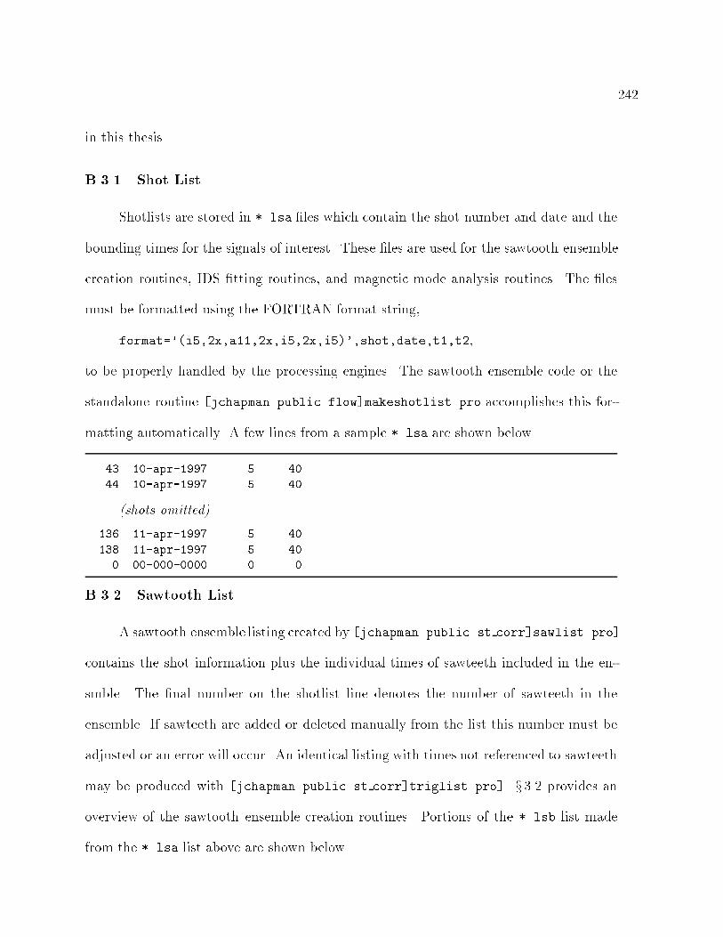
242

in this thesis.

B.3.1 Shot List

Shotlists are stored in *.lsa les which contain the shot number and date and the

bounding times for the signals of interest. These les are used for the sawtooth ensemble

creation routines, IDS tting routines, and magnetic mode analysis routines. The les

must be formatted using the FORTRAN format string,

format='(i5,2x,a11,2x,i5,2x,i5)',shot,date,t1,t2,

to be properly handled by the processing engines. The sawtooth ensemble code or the

standalone routine [jchapman.public.flow]makeshotlist.pro accomplishes this for-

matting automatically. A few lines from a sample *.lsa are shown below.

43 10-apr-1997 5 40

44 10-apr-1997 5 40

(shots omitted)

136 11-apr-1997 5 40

138 11-apr-1997 5 40

0 00-000-0000 0 0

B.3.2 Sawtooth List

A sawtooth ensemble listing created by [jchapman.public.st corr]sawlist.pro]

contains the shot information plus the individual times of sawteeth included in the en-

smble. The nal number on the shotlist line denotes the number of sawteeth in the

ensemble. If sawteeth are added or deleted manually from the list this number must be

adjusted or an error will occur. An identical listing with times not referenced to sawteeth

may be produced with [jchapman.public.st corr]triglist.pro]. x 3.2 provides an

overview of the sawtooth ensemble creation routines. Portions of the *.lsb list made

from the *.lsa list above are shown below.

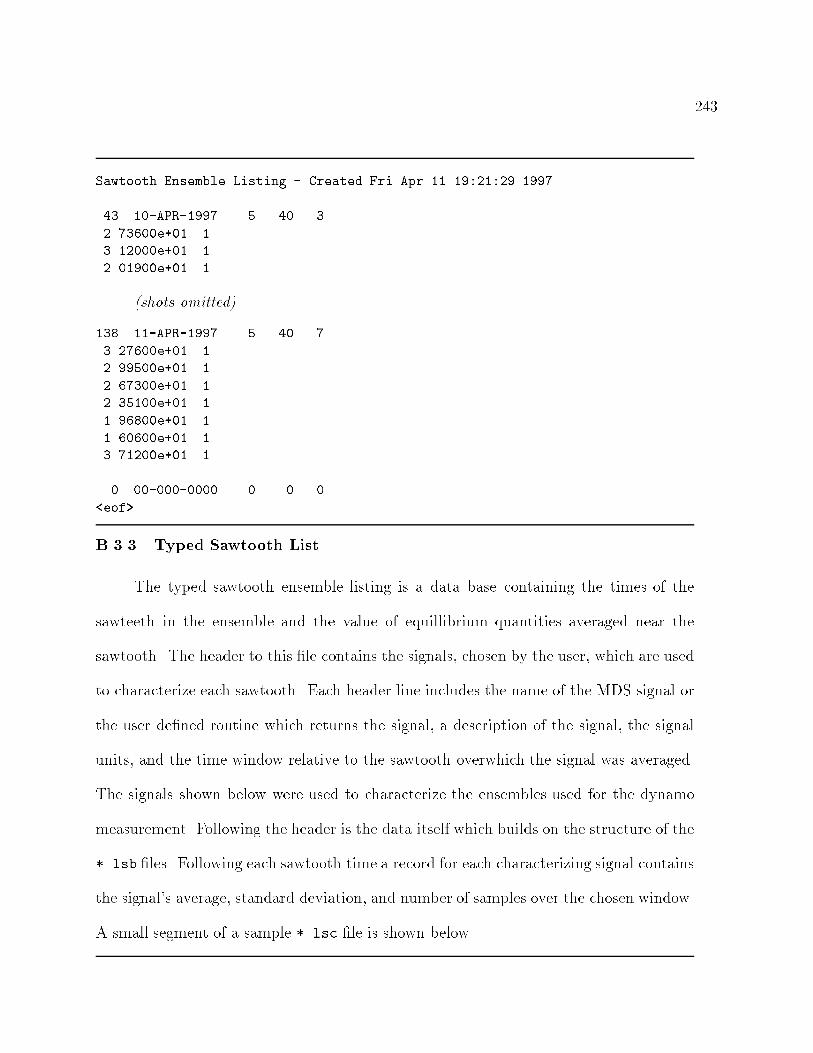
243

Sawtooth Ensemble Listing - Created Fri Apr 11 19:21:29 1997

43 10-APR-1997 5 40 3

2.73600e+01 1

3.12000e+01 1

2.01900e+01 1

(shots omitted)

138 11-APR-1997 5 40 7

3.27600e+01 1

2.99500e+01 1

2.67300e+01 1

2.35100e+01 1

1.96800e+01 1

1.60600e+01 1

3.71200e+01 1

0 00-000-0000 0 0 0

<eof>

B.3.3 Typed Sawtooth List

The typed sawtooth ensemble listing is a data base containing the times of the

sawteeth in the ensemble and the value of equillibrium quantities averaged near the

sawtooth. The header to this le contains the signals, chosen by the user, which are used

to characterize each sawtooth. Each header line includes the name of the MDS signal or

the user dened routine which returns the signal, a description of the signal, the signal

units, and the time window relative to the sawtooth overwhich the signal was averaged.

The signals shown below were used to characterize the ensembles used for the dynamo

measurement. Following the header is the data itself which builds on the structure of the

*.lsb les. Following each sawtooth time a record for each characterizing signal contains

the signal's average, standard deviation, and number of samples over the chosen window.

A small segment of a sample *.lsc le is shown below.

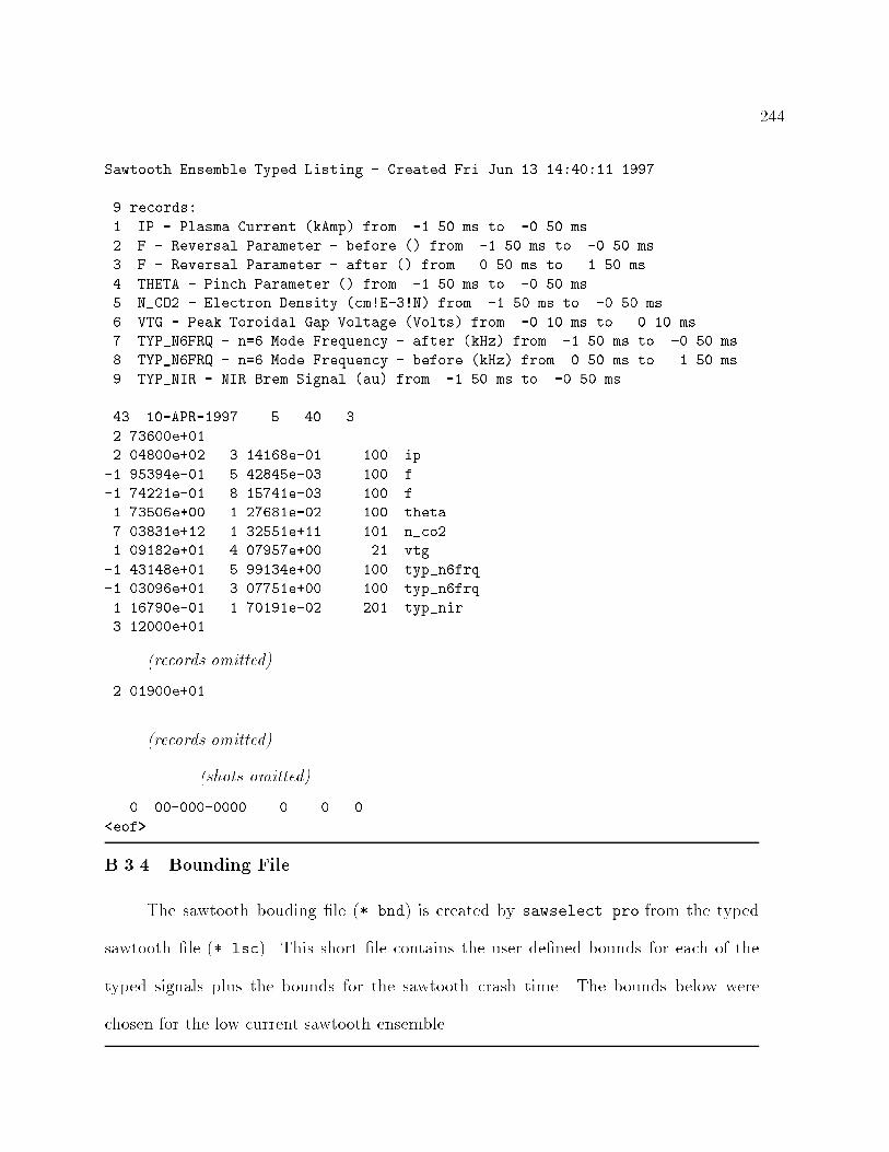
244

Sawtooth Ensemble Typed Listing - Created Fri Jun 13 14:40:11 1997

9 records:

1 IP - Plasma Current (kAmp) from -1.50 ms to -0.50 ms

2 F - Reversal Parameter - before () from -1.50 ms to -0.50 ms

3 F - Reversal Parameter - after () from 0.50 ms to 1.50 ms

4 THETA - Pinch Parameter () from -1.50 ms to -0.50 ms

5 N_CO2 - Electron Density (cm!E-3!N) from -1.50 ms to -0.50 ms

6 VTG - Peak Toroidal Gap Voltage (Volts) from -0.10 ms to 0.10 ms

7 TYP_N6FRQ - n=6 Mode Frequency - after (kHz) from -1.50 ms to -0.50 ms

8 TYP_N6FRQ - n=6 Mode Frequency - before (kHz) from 0.50 ms to 1.50 ms

9 TYP_NIR - NIR Brem Signal (au) from -1.50 ms to -0.50 ms

43 10-APR-1997 5 40 3

2.73600e+01

2.04800e+02 3.14168e-01 100 ip

-1.95394e-01 5.42845e-03 100 f

-1.74221e-01 8.15741e-03 100 f

1.73506e+00 1.27681e-02 100 theta

7.03831e+12 1.32551e+11 101 n_co2

1.09182e+01 4.07957e+00 21 vtg

-1.43148e+01 5.99134e+00 100 typ_n6frq

-1.03096e+01 3.07751e+00 100 typ_n6frq

1.16790e-01 1.70191e-02 201 typ_nir

3.12000e+01

(records omitted)

2.01900e+01

(records omitted)

(shots omitted)

0 00-000-0000 0 0 0

<eof>

B.3.4 Bounding File

The sawtooth bouding le (*.bnd) is created by sawselect.pro from the typed

sawtooth le (*.lsc). This short le contains the user dened bounds for each of the

typed signals plus the bounds for the sawtooth crash time. The bounds below were

chosen for the low current sawtooth ensemble.

245

Sawtooth Ensemble Bound File created on Mon Jun 16 13:13:24 1997

Sawtooth Ensemble Typed Listing - Created Fri Jun 13 14:40:11 1997

10

time of sawtooth crash (ms)

1.00000e+01 3.50000e+01

IP - Plasma Current (kAmp) from -1.50 ms to -0.50 ms

1.90000e+02 2.20000e+02

F - Reversal Parameter - before () from -1.50 ms to -0.50 ms

-2.20000e-01 -1.90000e-01

F - Reversal Parameter - after () from 0.50 ms to 1.50 ms

-1.90000e-01 -1.60000e-01

THETA - Pinch Parameter () from -1.50 ms to -0.50 ms

1.71000e+00 1.77000e+00

N_CO2 - Electron Density (cm!E-3!N) from -1.50 ms to -0.50 ms

6.50000e+12 8.00000e+12

VTG - Peak Toroidal Gap Voltage (Volts) from -0.10 ms to 0.10 ms

5.00000e+00 3.00000e+01

TYP_N6FRQ - n=6 Mode Frequency - after (kHz) from -1.50 ms to -0.50 ms

-2.50000e+01 -1.30000e+01

TYP_N6FRQ - n=6 Mode Frequency - before (kHz) from 0.50 ms to 1.50 ms

-2.00000e+01 -8.00000e+00

TYP_NIR - NIR Brem Signal (au) from -1.50 ms to -0.50 ms

7.00000e-02 1.70000e-01

B.4 Sawtooth Ensemble Analysis

B.4.1 Signal Routine

This signal routine was designed to be called by the sawtooth correlation routines.

The procedure returns uctuating velocity signals and ve toroidal magnetic modes. The

format of the passed values must be adhered to for all user dened signal routines.

;;;;==================================================================

pro SIG_VXB,shot,date,t1,t2,t,x,s,name,units,tlag

;;;;------------------------------------------------------------------

;;;; This signal routine is employed in the correlation of velocity fluct-

;;;; uations with the magnetic array. The signals are high-pass filtered

246

;;;; to reduce contamination of secular components into the signal. No

;;;; noise filtering was employed for fear of losing fast fluctuation power.

;;;; The data is correlated with the cosine amplitude of the n=5-9 modes

;;;; J. T. Chapman University of Wisconsin - Madison July 14, 1996

;;;;==================================================================

;;;-------------------------------------------------------------------

;;; Preliminary setup of data base and data arrays

;; setting up mds data base

set_db,'mst$data'

dummy=set_shot(shot)

dummy=set_date(date)

;; initializing time and frequency arrays

fsig=100.0 ;...output signal frequency

nn=fix((t2-t1)*fsig+1.5) ;...length of ouput array

t=findgen(nn)/fsig+t1 ;...time axis for output array

nf=(nn/256+1)*256 ;...length of buffered frequency axis

f=findgen(nf)*fsig/nf ;...frequency axis

f(nf/2+1:nf-1)=reverse(f(1:nf/2-1))

;; setting up filter cuttoffs

cut_noise=45.0 ;...noise above 45 kHz

cut_secular=3.0 ;...secular change below 3kHz

s_n=where(f ge cut_noise) ;...subscripts of noise spectrum

s_s=where(f le cut_secular) ;...subscripts of secular specturum

;; initializing data arrays

mag_modes=[10,11,12,13,14] ;...magnetic modes with which to corr.

;mag_modes=[5,6,7,8,9] ;...magnetic modes with which to corr.

;mag_modes=[1,2,3,4,15] ;...magnetic modes with which to corr.

n_mm=n_elements(mag_modes) ;...number of magnetic modes

n_sig=n_mm+2 ;...number of signals

x=fltarr(nn,n_sig) ;...signal array

247

name=strarr(n_sig) ;...name array

name(0)="Toroidal Ion Velocity"

name(1)="Poloidal Ion Velocity"

for i_m=0,n_mm-1 do begin

name(i_m+2)="n="+strtrim(mag_modes(i_m),2)+" Cosine Amplitude"

endfor

units=strarr(n_sig) ;...units array

units(0:1)="km/s"

units(2:n_sig-1)="gauss"

s=fltarr(n_sig) ;...error array

tlag=fltarr(n_sig) ;...time lag array

;;;-------------------------------------------------------------------

;;; Reading in velocity signals

;; aquiring signals from data base

tv=data('vfs_time')-3.64e-3 ;...reading in time record for velocity

nv=n_elements(tv)

if (nv le 1) then goto,SkipShot

n1v=min(where(tv ge t1)) ;...boundaries of time signal

n2v=max(where(tv le t2))

if ((n1v eq -1) or (n2v eq -1)) then goto,SkipShot

tv=tv(n1v:n2v)

;...reading in centroids

fit1_tor=(data('vfs_222_fit1')>0.0)<5.0

if (n_elements(fit1_tor) le 1) then goto,SkipShot

fit1_pol=(data('vfs_138_fit1')>0.0)<5.0

if (n_elements(fit1_pol) le 1) then goto,SkipShot

;; converting centroids to velocities

x_lam = 1.88238 ;...calibrated position of line

lam_0 = 2270.90 ;...impurity wavelength

;...Doppler formula!

vel_tor= 2.998e+5/lam_0*(x_lam-fit1_tor)

vel_pol=-2.998e+5/lam_0*(x_lam-fit1_pol)

;...keeping invalid points set to zero

248

if (min(fit1_pol) le 0.0) then vel_pol(where(fit1_pol le 0.0))=0.0

if (min(fit1_tor) le 0.0) then vel_tor(where(fit1_tor le 0.0))=0.0

;; cleaning up signals

;...zeroing outliers

vel_pol=clean(vel_pol,m=20,tol=5)

vel_tor=clean(vel_tor,m=20,tol=5)

;...too many zeros?

pcnt_bad=max([n_elements(where(vel_pol(n1v:n2v) eq 0.0)),$

n_elements(where(vel_tor(n1v:n2v) eq 0.0))])$

/float(n2v-n1v+1)

if (pcnt_bad ge 0.1) then goto,SkipShot

;...filling in zeros with nn routine

vel_pol=zerofill(vel_pol,tol=1.0e-6)

vel_tor=zerofill(vel_tor,tol=1.0e-6)

;; filtering velocity signals

;...measuring noise level

f_vel_pol=fft([vel_pol(n1v:n2v),fltarr(nf-n2v+n1v-1)],-1)

vel_pol_sig=sqrt(nf*total(abs(f_vel_pol(s_n))^2)/(n_elements(s_n)+1))

f_vel_tor=fft([vel_tor(n1v:n2v),fltarr(nf-n2v+n1v-1)],-1)

vel_tor_sig=sqrt(nf*total(abs(f_vel_tor(s_n))^2)/(n_elements(s_n)+1))

f_vel_pol(s_s)=0.0 ;...filtering out secular component

vel_pol_fil=extrac(float(fft(f_vel_pol,1)),n1v,n2v-n1v+1)

f_vel_tor(s_s)=0.0

vel_tor_fil=extrac(float(fft(f_vel_tor,1)),n1v,n2v-n1v+1)

;; placing velocity signals in data array

n1x=max(where(min(abs(t-tv(0))) eq abs(t-tv(0))))

n2x=(n1x+n_elements(tv)-1)<nn

n2v=n2x-n1x

x(n1x:n2x,0)=vel_tor_fil(0:n2v)

x(n1x:n2x,1)=vel_pol_fil(0:n2v)

tlag(0:1)=avg(tv(0:n2v)-t(n1x:n2x))

;;;-------------------------------------------------------------------

;;; Acquiring magnetics

tm=data('modes_time')*1000.

249

nm=n_elements(tm)/2

if (nm le 1) then goto,SkipShot

tm=rebin(tm(0:nm*2-1),nm)

n1m=min(where(tm ge t1)) ;...boundaries of time signal

n2m=max(where(tm le t2))

if ((n1m eq -1) or (n2m eq -1)) then goto,SkipShot

n1x=max(where(min(abs(t-tm(n1x))) eq abs(t-tm(n1x))))

n2x=(n1x+n2m-n1m)<nn

n2m=(n1m+n2x-n1x)

for i_m=0,n_mm-1 do begin

cos_amp=data('modes_'+strtrim(mag_modes(i_m),2)+'_cos')

if (n_elements(cos_amp) le 1) then goto,SkipShot

cos_amp=rebin(cos_amp(0:nm*2-1),nm)

;...filtering out secular component

f_cos_amp=fft([cos_amp(n1m:n2m),fltarr(nf-n2m+n1m-1)],-1)

f_cos_amp(s_s)=0.0

cos_amp=extrac(float(fft(f_cos_amp,1)),n1m,n2m-n1m+1)

x(n1x:n2x,i_m+2)=cos_amp

endfor

tlag(2:n_mm+1)=avg(tm(n1m:n2m)-t(n1x:n2x))

;;;-------------------------------------------------------------------

return

SkipShot:

t=-1 & x=-1

return

end

B.4.2 Averaging Routine

This ensemble average routine conducts one pass through the ensemble calculating

the signal averages, variance, and power spectra. No correlations between the signals is

performed A description of the algorithms in this routine may be found in x 3.2.

250

;;;;==================================================================

;;;;

;;;; ST_AVER.PRO

;;;;

;;;; This routine is a simplified version of ST_CORR. It performs one

;;;; pass through the ensemble and returns the average and power spectra

;;;; of the windowed signals. No cross products or spectra are calcu-

;;;; lated. In all other ways this routine is setup in an identically

;;;; to ST_CORR.PRO. If you have the sawtooth ensemble for ST_CORR

;;;; you do NOT have to redo it for ST_AVER (and vice-versa).

;;;;

;;;; J. T. Chapman University of Wisconsin - Madison 10/21/96

;;;;==================================================================

;;; Hello and Welcome to the Sawtooth Correlation Routine

print, format='(80("="))'

print, ' '

print, 'Sawtooth Window Averaging Routine'

print, ' '

print, format='(80("-"))'

print, ' '

print, ' Main Level Variables'

print, ' working directory: '+!working_dir

if (strlen(save_file) eq 0) then $

print, ' idl save file: '+'<none>' $

else $

print, ' idl save file: '+save_file+'.DAT'

print, ' typed sawtooth listing: '+saw_list_file+'.LSC'

print, ' sawtooth bounding file: '+sel_list_file+'.LSC'

print, ' signal routine: '+signal+'.PRO'

print, ' time before crash: '+strtrim(prewin,2)+' ms'

print, ' time after crash: '+strtrim(poswin,2)+' ms'

if verbose then $

print, ' verbose: 1 (progress messages on)' $

else $

print, ' verbose: 0 (progress messages off)'

print, ' '

print, format='(80("-"))'

print, ' '

;=====================================================================

; looping through two passes

251

init = 1 ;...raising initialization flag

;...opening sawtooth list file

safe_openr,saw_list_file,saw_lun,ext='lsc',dir=!working_dir

;...opening sawtooth selection file

safe_openr,sel_list_file,sel_lun,ext='bnd',dir=!working_dir

;---------------------------------------------------------------------

; starting shot loop

point_lun,saw_lun,0 ;...rewinding sawtooth listing

dummy=" " ;...reading off header of sawlist file

readf,saw_lun,dummy & readf,saw_lun,dummy

n_records=0

readf,saw_lun,n_records

for i=0,n_records-1 do readf,saw_lun,dummy

shot=0 ;...current shot, 0 for stop processing

date='00-xxx-0000' ;...date of shot

t1=0 ;...start time of shot

t2=0 ;...end time of shot

;...reading in first shot

SHOT_SET,saw_lun,sel_lun,shot,date,t1,t2,t_crash

while (shot ne 0) do begin ;...main shot loop

;...checking sawteeth windows

vc=where(((t_crash-prewin) ge t1) and ((t_crash+poswin) le t2))

if (max(vc) eq -1) then goto,SkipShot else t_crash=t_crash(vc)

if verbose then $

print,format='($," ",a)',strtrim(filecode(shot,date),2) $

else print," Shot "+strtrim(shot,2)+" on "+date

;---------------------------------------------------------------------

; obtaining user signals, characterizing basic parameters

if verbose then print,format='($,"...reading")'

;...reading in signal from user function

252

call_procedure,signal,shot,date,t1,t2,t,x,sx,name,units,tlag

sig_size = size(x) ;...characterizing signal geometry

;...skipping shot with missing data

if (sig_size(0) eq 0) then goto, SkipShot

lsig = sig_size(1) ;...length of signal

if init then nsig=sig_size(2) ;...number of signals

dt=(max(t)-min(t))/(lsig-1) ;...time resolution

sig_val=fltarr(nsig)+1 ;...sig_val defaults to true

for i=0,nsig-1 do if (avg(x(*,i)^2) eq 0.0) then sig_val(i)=0.0

;---------------------------------------------------------------------

; intialization of arrays

if ( init ) then begin ;...if initializing necessary

;...number of points in window

nw=fix((prewin+poswin)/dt+1.5)

dxav = fltarr(nw,nsig) ;...average sawtooth profile

dxdxav = fltarr(nw,nsig) ;...average fluctuation product

sxav = fltarr(nsig) ;...average random power

sxsxav = fltarr(nsig) ;...average random (power)^2

dfdfav = fltarr(nw,nsig) ;...spectra of fluctuation products

sfav = fltarr(nw,nsig) ;...average random spectral power

sfsfav = fltarr(nw,nsig) ;...average random (spectral power)^2

;...creating time and frequency axis

taxis = findgen(nw)*dt-prewin

faxis = findgen(nw/2+1)/(nw*dt)

npre = fix((nw-1)*(float(prewin)/(prewin+poswin))+0.5)

npos = fix((nw-1)*(float(poswin)/(prewin+poswin))+0.5)

nevent = intarr(nw,nsig) ;...number of sawtooth events

init = 0 ;...lowering init flag

253

endif

;---------------------------------------------------------------------

; sawtooth ensemble loop

n_crash=n_elements(t_crash) ;...number of sawtooth crashes

if verbose then print,"..."+strtrim(n_crash,2)+" events."

for i_crash = 0, n_crash-1 do begin

n0 = max(where(min(abs(t-t_crash(i_crash))) eq $

abs(t-t_crash(i_crash)) ))

n1 = (n0-npre)>0

n2 = (n0+npos)<(lsig-1)

n1d = (npre-n0+n1)>0

n2d = (npre-n0+n2)<(nw-1)

dx = fltarr(nw,nsig) ;...initializing sawtooth arrays

for i=0,nsig-1 do begin ;...filling sawtooth arrays

if sig_val(i) then begin

dx(n1d:n2d,i) = x(n1:n2,i)

nevent(n1d:n2d,i) = nevent(n1d:n2d,i)+1

endif

endfor

;---------------------------------------------------------------------

; calculating average profiles

dxav = dxav + dx ;...updating average profile

dxdxav = dxdxav + dx^2

sxav = sxav + sx^2 ;...updating average errors

sxsxav = sxsxav + sx^4

;---------------------------------------------------------------------

; calculating spectral quantities (second pass)

w = hanning(nw) ;...windowing array

if spec_calc then begin

254

;...calculating transforms

df = complexarr( nw, nsig )

for i=0,nsig-1 do if sig_val(i) then $

df(*,i) = fft( dx(*,i)*w-avg(dx(*,i)*w), -1 )

;...estimating power spectra

dfdfav = dfdfav + abs(df)^2.

;...average random power^2

for i=0,nsig-1 do if sig_val(i) then begin

sfav(*,i) = sfav(*,i) + sx(i)^2*abs(df(*,i))^2 $

/ total(abs(df(*,i))^2)

sfsfav(*,i) = sfsfav(*,i) + ( sx(i)^2*abs(df(*,i))^2 $

/ total(abs(df(*,i))^2) )^2

endif

endif

;--------------------------------------------------------------------

SkipCrash:

endfor ;...end of sawtooth averaging loop

;--------------------------------------------------------------------

; wrapping up shot ensemble loop

SkipShot:

;...getting next shot

SHOT_SET,saw_lun,sel_lun,shot,date,t1,t2,t_crash

endwhile ;...end of shot ensemble loop

;---------------------------------------------------------------------

; normalizing ensemble quantities

for isig=0,nsig-1 do begin

vv=where(nevent(*,isig))

if (max(vv) ne -1) then begin

dxav(vv,isig) = dxav(vv,isig) / nevent(vv,isig)

dxdxav(vv,isig) = dxdxav(vv,isig) / nevent(vv,isig)

255

sxav(isig) = sxav(isig) / max(nevent(vv,isig))

sxsxav(isig) = sxsxav(isig) / max(nevent(vv,isig))

endif

endfor

dfdfav = dfdfav(0:nw/2,*) ;...converting to one-sided spectra

sfav = sfav(0:nw/2,*)

sfsfav = sfsfav(0:nw/2,*)

;...normalizing average spectra

norm_win = [1.0,fltarr(nw/2-1)+2.0,1.0]

for i=0,nsig-1 do if (max(nevent(*,i)) ne 0) then begin

dfdfav(*,i) = dfdfav(*,i) * norm_win / avg(w^2)/max(nevent(*,i))

sfav(*,i) = sfav(*,i) * norm_win / max(nevent(*,i))

sfsfav(*,i) = sfsfav(*,i) * norm_win / max(nevent(*,i))

endif

; calculating errors

;...error in average products

sdxav=fltarr(nsig)

sdxdxav=fltarr(nsig)

for ii=0,nsig-1 do if (max(nevent(*,ii)) ne 0) then begin

sdxav(ii) = sqrt(sxav(ii)/max(nevent(*,ii)))

sdxdxav(ii) = sqrt(2*sxsxav(ii)/max(nevent(*,ii)))

endif

;...error in average spectra

sdfdfav=fltarr(nw/2+1,nsig)

; for ii=0,nsig-1 do if (max(nevent(*,ii) ne 0) then begin

; sdfdfav(*,ii,ii) = sqrt((2*dfdfav(*,ii,ii)*sfav(*,ii) + $

; sfsfav(*,ii,ii))/max(nevent(*,ii,jj)))

; endif

;=====================================================================

; fluctation correlation routine wrap-up

;...write variables do save file

if (strlen(strtrim(save_file,2)) ne 0) then $

save,file=!working_dir+save_file,$

taxis,faxis,dxav,sdxav,dxdxav,sdxdxav,sxav,sxsxav,$

dfdfav,sdfdfav,sfav,sfsfav, $

256

nevent,nsig,dt,nw,name,units,tlag

free_lun,saw_lun,sel_lun ;...freeing logical units

;...say Goodbye

print," "

print,"Goodbye."

print," "

print,format='(80("="))'

end ;...FINE!

;=====================================================================

B.4.3 Wavelet Analysis Routine

This correlation engine performs two passes through the sawtooth ensemble. The

details of the algorithms employed may be found in x 3.2. This engine is identical to

st corr but has added ensemble wavelet analysis.

;;;;==================================================================

;;;;

;;;; ST_WVLT.PRO

;;;;

;;;; This routine finds the correlation and coherence of an ensemble of

;;;; windowed signals provided by the user. The routine loops twice through

;;;; the ensemble. The first loop finds the average of the signals, the

;;;; second to analyzes the fluctuating part of subtracting the average.

;;;;

;;;; J. T. Chapman University of Wisconsin - Madison 10/21/96

;;;;

;;;; Wavelet analysis incorportated into sawtooth correlation routine.

;;;;

;;;; E. Martines Consorzio RFX - Padova, Italy 09/09/97

;;;;==================================================================

;;; Hello and Welcome to the Sawtooth Correlation Routine

print, format='(80("="))'

print, ' '

print, 'Sawtooth Window Fluctuation Correlation Routine'

print, ' '

257

print, format='(80("-"))'

print, ' '

print, ' Main Level Variables'

print, ' working directory: '+!working_dir

print, ' idl save file: '+save_file+'.DAT'

print, ' typed sawtooth listing: '+saw_list_file+'.LSC'

print, ' sawtooth bounding file: '+sel_list_file+'.BND'

print, ' signal routine: '+signal+'.PRO'

print, ' time before crash: '+strtrim(prewin,2)+' ms'

print, ' time after crash: '+strtrim(poswin,2)+' ms'

if verbose then $

print, ' verbose: 1 (progress messages on)' $

else $

print, ' verbose: 0 (progress messages off)'

print, ' '

print, format='(80("-"))'

print, ' '

;=====================================================================

; looping through two passes

;...raising initialization flag

init = 1

time_read = 0.0

time_calc = 0.0

;...opening sawtooth list file

safe_openr,saw_list_file,saw_lun,ext='lsc',dir=!working_dir

;...opening sawtooth selection file

safe_openr,sel_list_file,sel_lun,ext='bnd',dir=!working_dir

;...two pass outer loop

for ipass=1,2 do begin

;...pass message

if (ipass eq 1) then $

print,"First Pass: Mean Profile" $

else $

print,"Second Pass: Fluctuating Quantities"

print," "

;---------------------------------------------------------------------

258

; starting shot loop

point_lun,saw_lun,0 ;...rewinding sawtooth listing

dummy=" " ;...reading off header of sawlist file

readf,saw_lun,dummy & readf,saw_lun,dummy

n_records=0

readf,saw_lun,n_records

for i=0,n_records-1 do readf,saw_lun,dummy

shot=0 ;...current shot, 0 for stop processing

date='00-xxx-0000' ;...date of shot

t1=0 ;...start time of shot

t2=0 ;...end time of shot

;...reading in first shot

SHOT_SET,saw_lun,sel_lun,shot,date,t1,t2,t_crash

while (shot ne 0) do begin ;...main shot loop

;...checking sawteeth windows

vc=where(((t_crash-prewin) ge t1) and ((t_crash+poswin) le t2))

if (max(vc) eq -1) then goto,SkipShot else t_crash=t_crash(vc)

print," Shot "+strtrim(shot,2)+" on "+date+", "+strtrim(t1,2)+"-"+$

strtrim(t2,2)+" ms, "+strtrim(n_elements(t_crash),2)+" events."

;---------------------------------------------------------------------

; obtaining user signals, characterizing basic parameters

if verbose then print,format='($," ...reading")'

;...reading in signal from user function

dumt=systime(1)

call_procedure,signal,shot,date,t1,t2,t,x,sx,name,units,tlag

time_read=time_read+systime(1)-dumt

sig_size = size(x) ;...characterizing signal geometry

;...skipping shot with missing data

if (sig_size(0) eq 0) then goto, SkipShot

lsig = sig_size(1) ;...length of signal

nsig = sig_size(2) ;...number of signals

259

dt=(max(t)-min(t))/(lsig-1) ;...time resolution

;---------------------------------------------------------------------

; creating phase shifted signal

if verbose then print,format='($,"...phase shift")'

p = fltarr( lsig, nsig ) ;...phase shifted signal

lbuf=64-(lsig mod 64) ;...buffer for signal to factor of 64

phsft = fltarr( lbuf+lsig ) ;...phase shifting array

;...setting for 90 degree phase shift

phsft(0:(lbuf+lsig-1)/2) = 1.0

phsft((lbuf+lsig+1)/2:lbuf+lsig-1) = -1.0

;...recovering phase shifted signal

for isig=0,nsig-1 do $

p(*,isig) = temporary(extrac(float(fft( $

fft([fltarr(lbuf),x(*,isig)],-1) * complex(0,phsft), $

1)),lbuf,lsig))

;---------------------------------------------------------------------

; intialization of arrays

if ( init ) then begin ;...if initializing necessary

;...number of points in window

nw=fix((((prewin+poswin)/dt)+0.5)/2)*2

dx = fltarr(nw,nsig) ;...initializing sawtooth arrays

dp = fltarr(nw,nsig)

dxav = fltarr(nw,nsig) ;...average sawtooth profile

dpav = fltarr(nw,nsig) ;...average phase shifted sawtooth

;...average fluctuation product

dxdxav = fltarr(nw,nsig,nsig)

sxav = fltarr(nsig) ;...average random power

sxsxav = fltarr(nsig,nsig);...average random (power)^2

;...spectra of fluctuation products

260

dfdfav = fltarr(nw,nsig,nsig)

sfav = fltarr(nw,nsig) ;...average random spectral power

;...average random (spectral power)^2

sfsfav = fltarr(nw,nsig,nsig)

;...creating time and frequency axis

taxis = findgen(nw)*dt-prewin

faxis = findgen(nw/2+1)/(nw*dt)

;; Wavelet analysis array declarations

;...wavelet frequency axis

if (not defined(wfaxis)) then begin

if not defined(wfreqmin) then wfreqmin=4.0/(nw*dt)

if not defined(wfreqmax) then wfreqmax=1.0/(2*dt)

nwf=fix(2*!pi*alog(wfreqmax/wfreqmin))+1

wfaxis=wfreqmin*(wfreqmax/wfreqmin)^(findgen(nwf)/(nwf-1))

endif

;...frequency interval size

dwfaxis =(shift(wfaxis,-1)-shift(wfaxis,+1))/2.0

dwfaxis(0) =(wfaxis(1)-wfaxis(0))/2.0+wfaxis(0)/(2*!pi)

dwfaxis(nwf-1) =(wfaxis(nwf-1)-wfaxis(nwf-2))/2.0

dwfaxis =dwfaxis*(nw*dt)

fwav=fltarr(2*nw,nwf) ;...defining wavelets if Fourier space

wftemp=[findgen(nw+1),-reverse(findgen(nw-1)+1.0)]/(2*nw*dt)

for iwf=0,nwf-1 do begin

; wav = 1.0/(!pi/wfaxis(iwf)^2)^0.25 * $

; exp(-0.5*((t-t(0))*wfaxis(iwf))^2) * $

; complex( cos(2*!pi*(t-t(0))*wfaxis(iwf), $

; sin(2*!pi*(t-t(0))*wfaxis(iwf) )

; wav = [ wav, 0.0, reverse(conj(wav(1:*))) ]

261

; fwav(*,iwf) = fft(wav,-1)*(2*nw*dt)

fwav(*,iwf) = (4*!pi/wfaxis(iwf)^2)^0.25 * $

exp(-0.5*((wftemp/wfaxis(iwf)-1)*2*!pi)^2)

fwav(0,iwf) = 0.0

endfor

wftemp=0 ;...clearing array

;...wavelet coefficients

dw = complexarr(nw,nwf,nsig)

;...average wavelet coefficients

dwav = complexarr(nw,nwf,nsig)

;...average wavelet products

dwdwav = fltarr(nw,nwf,nsig,nsig)

nevent = 0 ;...number of sawtooth events

init = 0 ;...lowering init flag

endif

;---------------------------------------------------------------------

; sawtooth ensemble loop

n_crash=n_elements(t_crash) ;...number of sawtooth crashes

for i_crash = 0, n_crash-1 do begin

;...boudaries of sawtooth event

n1 = fix(min(where( t ge (t_crash(i_crash)-prewin) )))

n2 = nw+n1-1

for i=0,nsig-1 do begin ;...filling sawtooth arrays

dx(*,i) = x(n1:n2,i)

dp(*,i) = p(n1:n2,i)

endfor

;---------------------------------------------------------------------

; calculating average profiles (first pass)

if (ipass eq 1) then begin

262

dxav = dxav + dx ;...updating average profile

dpav = dpav + dp

sxav = sxav + sx^2 ;...updating average errors

for ii=0,nsig-1 do for jj=0,nsig-1 do $

sxsxav(ii,jj) = sxsxav(ii,jj) + sx(ii)^2*sx(jj)^2

nevent = nevent + 1 ;...updating number of events

endif

;---------------------------------------------------------------------

; subtracting average sawtooth profile from window (first pass)

if (ipass eq 2) then begin

for i=0,nsig-1 do begin ;...straight subtraction

dx(0:(n2-n1),i)=dx(0:(n2-n1),i)-dxav(0:(n2-n1),i)

dp(0:(n2-n1),i)=dp(0:(n2-n1),i)-dpav(0:(n2-n1),i)

endfor

endif

;---------------------------------------------------------------------

; calculating fluctuation products (second pass)

if (ipass eq 2) then $

for ii=0,nsig-1 do for jj=0,nsig-1 do begin

if (ii le jj) then $

dxdxav(*,ii,jj) = dxdxav(*,ii,jj) + dx(*,ii)*dx(*,jj)$

else $

dxdxav(*,ii,jj) = dxdxav(*,ii,jj) + dx(*,ii)*dp(*,jj)

endfor

;---------------------------------------------------------------------

; calculating spectral quantities (second pass)

w = hanning(nw) ;...windowing array

if ((ipass eq 2) and spec_calc) then begin

;...calculating transforms

263

df = complexarr( nw, nsig )

for i=0,nsig-1 do df(*,i) = fft( dx(*,i)*w, -1 )

;...estimating power spectra

for i=0,nsig-1 do $

dfdfav(*,i,i) = dfdfav(*,i,i) + abs(df(*,i))^2.

;...average cross spectra off diagonal

for i=0,nsig-2 do for j=i+1,nsig-1 do begin

dfdfav(*,i,j) = dfdfav(*,i,j) + float( df(*,i)*conj(df(*,j)))

dfdfav(*,j,i) = dfdfav(*,j,i) + imaginary(df(*,i)*conj(df(*,j)))

endfor

;...average random power

for i=0,nsig-1 do $

sfav(*,i) = sfav(*,i) + sx(i)^2*abs(df(*,i))^2 $

/ total(abs(df(*,i))^2)

;...average random power^2

for i=0,nsig-1 do for j=0,nsig-1 do $

sfsfav(*,i,j) = sfsfav(*,i,j) $

+ sx(i)^2*sx(j)^2*abs(df(*,i))^2*abs(df(*,j))^2$

/ total(abs(df(*,i))^2)*total(abs(df(*,j))^2)

endif

;---------------------------------------------------------------------

; calculating wavelet coefficients

if (ipass eq 2) then begin

dumt=systime(1)

;...calculating wavelet transform (fwav is real)

for isig=0,nsig-1 do begin

fsig=fft([dx(*,isig),replicate(0.0,nw)],-1)

for iwf=0,nwf-1 do $

dw(*,iwf,isig)=extrac(fft(fwav(*,iwf)*fsig,1),0,nw)

fsig=0

endfor

dwav=dwav+dw ;...averaging wavelet coefficients

264

;...averaging wavelet products

for i=0,nsig-1 do $

dwdwav(*,*,i,i) = dwdwav(*,*,i,i) + abs(dw(*,*,i))^2

for i=0,nsig-2 do for j=i+1,nsig-1 do begin

dwdwav(*,*,i,j) = dwdwav(*,*,i,j) + $

float( dw(*,*,i)*conj(dw(*,*,j)) )

dwdwav(*,*,j,i) = dwdwav(*,*,j,i) + $

imaginary( dw(*,*,i)*conj(dw(*,*,j)) )

endfor

time_calc=time_calc+systime(1)-dumt

endif

;---------------------------------------------------------------------

endfor ;...end of sawtooth averaging loop

;---------------------------------------------------------------------

; wrapping up shot ensemble loop

SkipShot:

;...getting next shot

SHOT_SET,saw_lun,sel_lun,shot,date,t1,t2,t_crash

endwhile ;...end of shot ensemble loop

;---------------------------------------------------------------------

; normalizing ensemble quantities

;...average profiles and errors

if (ipass eq 1) then begin

dxav = dxav/nevent

dpav = dpav/nevent

sxav = sxav/nevent

sxsxav = sxsxav/nevent

endif

;...average products and spectra

if (ipass eq 2) then begin

dxdxav = dxdxav/nevent ;...normaling average products

dfdfav = dfdfav(0:nw/2,*,*) ;...converting to one-sided spectra

sfav = sfav(0:nw/2,*)

265

sfsfav = sfsfav(0:nw/2,*,*)

;...normalizing average spectra

norm_win = [1.0,fltarr(nw/2-1)+2.0,1.0]/nevent

for i=0,nsig-1 do sfav(*,i) = sfav(*,i)*norm_win

for i=0,nsig-1 do for j=0,nsig-1 do begin

dfdfav(*,i,j) = dfdfav(*,i,j)*norm_win/avg(w^2)

sfsfav(*,i,j) = sfsfav(*,i,j)*norm_win

endfor

dwdwav = dwdwav/(2*nevent) ;...normalizing wavelet products

dwav = dwav/nevent ;...normalizing wavelet coefficients

endif

;---------------------------------------------------------------------

; end of two-pass super loop

print," "

endfor

;=====================================================================

; calculating ensemble quantities

print," "

print,"Calculating Ensemble Quantities"

;---------------------------------------------------------------------

; calculating errors

sdxav=sqrt(sxav/nevent) ;...error in average profile

;...error in average products

sdxdxav=fltarr(nsig,nsig)

for ii=0,nsig-1 do for jj=0,nsig-1 do $

if (ii eq jj) then $

sdxdxav(ii,ii)=sqrt(2*sxsxav(ii,ii))/sqrt(nevent) $

else $

sdxdxav(ii,jj)=sqrt(sxsxav(ii,jj))/sqrt(nevent)

;...error in average spectra

sdfdfav=fltarr(nw/2+1,nsig,nsig)

; for ii=0,nsig-1 do for jj=0,nsig-1 do $

266

; if (ii eq jj) then $

; sdfdfav(*,ii,ii)=sqrt(2*dfdfav(*,ii,ii)*sfav(*,ii)+sfsfav(*,ii,ii))$

; / sqrt(nevent) $

; else $

; sdfdfav(*,ii,jj)=sqrt(sfsfav(*,ii,jj)+dfdfav(*,ii,ii)*sfav(*,jj) $

; + dfdfav(*,jj,jj)*sfav(*,ii))/sqrt(2*nevent)

;---------------------------------------------------------------------

; calculating correlation array

correlation=0

if ens_calc then begin

;...initializing arrays

correlation = fltarr( nw, nsig, nsig )

;...looping pairwise through signals

for i=0,nsig-2 do for j=i+1,nsig-1 do begin

;...trick to avoid dividing by zero

base=sqrt( dxdxav(*,i,j)^2 + dxdxav(*,j,i)^2 )

base=min(base(where(base ne 0.0)))*0.1

;...calculating correlation

correlation(*,i,j) = $

sqrt( dxdxav(*,i,j)^2 + dxdxav(*,j,i)^2 )/ $

(sqrt( abs( dxdxav(*,i,i) * dxdxav(*,j,j) ) )>base)

;...estimating average phase of signals

correlation(*,j,i) = atan(dxdxav(*,j,i),dxdxav(*,i,j))

endfor

endif

;---------------------------------------------------------------------

; calculating coherence array

coherence=0

if (ens_calc and spec_calc) then begin

;...initializing coherence arrays

coherence = fltarr(nw/2+1,nsig,nsig)

267

;...looping pairwise through signals

for i=0,nsig-2 do for j=i+1,nsig-1 do begin

;...trick to avoid dividing by zero

base=sqrt( abs( dfdfav(*,i,i) )*abs( dfdfav(*,j,j) ) )

base=min(base(where(base ne 0.0)))*0.1

;...calculating coherence array

coherence(*,i,j) = $

sqrt( dfdfav(*,i,j)^2 + dfdfav(*,j,i)^2 ) / $

sqrt( abs( dfdfav(*,i,i) * dfdfav(*,j,j) ) >base)

;...calculation of phase angle

coherence(*,j,i) = atan( dfdfav(*,j,i),dfdfav(*,i,j) )

endfor

endif

;---------------------------------------------------------------------

; calculating wavelet coherence array

wcoherence=0

if (ens_calc and spec_calc) then begin

;..initializing wavelet coherence arrays

wcoherence = fltarr(nw,nwf,nsig,nsig)

;...looping pairwise through signals

for i=0,nsig-2 do for j=i+1,nsig-1 do begin

;...trick to avoid dividing by zero

base=sqrt( abs( dwdwav(*,*,i,i) )*abs( dwdwav(*,*,j,j) ) )

base=min(base(where(base ne 0.0)))*0.1

;...calculating wavelet coherence array

wcoherence(*,*,i,j) = $

sqrt( dwdwav(*,*,i,j)^2 + dwdwav(*,*,j,i)^2 ) / $

sqrt( abs( dwdwav(*,*,i,i) * dwdwav(*,*,j,j) ) >base)

;...calculation of wavelet phase angle

wcoherence(*,*,j,i) = atan( dwdwav(*,*,j,i),dwdwav(*,*,i,j) )

endfor

268

for i=0,nsig-1 do $

wcoherence(*,*,i,i)=atan(imaginary(dwav(*,*,i)), $

float(dwav(*,*,i)) )

endif

;=====================================================================

; fluctation correlation routine wrap-up

;...write variables do save file

if (not (defined(save_xdr))) then save_xdr=0

if (strlen(strtrim(save_file,2)) ne 0) then $

save,file=!working_dir+save_file,xdr=save_xdr,$

taxis,faxis,wfaxis,dxav,dpav,sdxav,dxdxav,sdxdxav, $

sxav,sxsxav,dfdfav,sdfdfav,sfav,sfsfav,dwdwav,dwfaxis, $

coherence,wcoherence,correlation, $

nevent,nsig,dt,nw,name,units,tlag,time_calc,time_read,nwf

free_lun,saw_lun,sel_lun

print," " ;...say Goodbye

print,"Goodbye."

print," "

print,format='(80("="))'

end ;...FINE!

;=====================================================================

B.5 Magnetic Mode Analysis

The noninteractive routine modes b.com serves as the front end for the IDS t

engine. The user denes the variables in this le and submits the job to a VMS batch

queue. The batch routine then denes the necessary variables, compiles the subroutines,

and calls the main mode analysis engine.

$ set def [jchapman.public.mode_anal]

$ idl

;;;===================================================================

269

;;; MODES_B.COM

;;;; This is an IDL batch routine designed simply to compile

;;;; the subroutines and initialize the variables necessary to run

;;;; MODES.PRO, the primary mode analysis engine. It is recommended

;;;; that users copy this batch file into their directory where they

;;;; can modify it according to their needs. It is not necessary to

;;;; copy MODES.PRO which is designed to run out of the public directory.

;;;; Any questions or comments regarding the routines in this directory

;;;; should be directed to Jim Chapman (jchapman@juno.physics.wisc.edu).

;;;; J. T. ChapmanUniversity of Wisconsin - Madison May 22, 1997

;;;;==================================================================

;; Compiling necessary subroutines.

.run [jchapman.idl]deriv_5pt

.run [jchapman.idl]defined

.run [jchapman.idl]thinn

.run [jchapman.idl]vtt

;; Specifying input files

;...The shot list is a list of shots, dates, starting

; and ending times input by the modes analysis.

; Such a list may easily be made by running the

; routine MAKESHOTLIST from this directory. These

; lists have a .LSA suffix and are identical to the

; shotlist produced by the correlation routines.

; A shot file MUST be specified for the routine to

; run on your data.

shot_file = "[myname.mydirectory]myshotlist.lsa"

;...The renormalization file contains the current

; renormalization for the magnetic coil array.

; If left undefined the routine will use the default

; renormalizations in this directory which I will

; attempt to keep current. To create you own

; renormalization file run RENORM_CALC from this

; directory.

renorm_file = "[myname.mydirectory]myrenormfile.dat"

;; Specifying run variables

;...n is an integer array of the toroidal mode numbers

; for which you wish to calculate amplitudes. If

270

; left undefined the routine defaults to calculating

; modes 5, 6, 7, and 8.

n = [ 5, 6, 7, 8]

;...ncb is an integer specifying the nuber of coils

; used for toroidal mode analysis. MODES will

; work with 16, 32, or 64 coils. If left undefined

; ncb defaults to 32 coil analysis.

ncb = 32

;...v_sat_hi and v_sat_lo are the digitizer saturation

; voltages. These may be either a single value if

; the saturation voltages are all the same or an

; array ncb long if digitizers with different

; saturation voltages are used. If left undefined

; v_sat_hi defaults to 2.5 and v_sat_lo to -2.5.

; (See note on signal order below if specifying

; saturation levels for each digitizer.)

v_sat_hi = +5.0

v_sat_lo = -5.0

;...output_freq is the frequency at which the mode

; amplitudes are output to the data base. The

; toroidal array is digitized at 200kHz. The modes

; may therefore be written at 200kHz, 100kHz, 66kHz,

; 50kHz, 40kHz, 33kHz, 25kHz, and 10kHz. The routine

; defaults to 100kHz

output_freq = 100

;...plot_vel determines whether the n=6 mode velocity

; will be plotted as the processing continues. This

; should only be set to 1 if the mode analysis is

; being done interactively. Plot_vel defaults to 0.

plot_vel = 0

;...bpgain sets the integrator gain for MODES. This

; may be set to a single integer gain if all gains

; are identical or an array if different coils have

; different integrator gains. If bpgain is set to 0

; the routine assumes that the shot_file also

; contains the integrator gains. Such a set up is

; useful if the gains change during a run. A shot

; list with the gains may be created by running

; CHECK_GAINS from this directory after creating

; a normal list with MAKESHOTLIST. If left undefined

; bpgain defaults to 20.

271

; (See note on signal order below if specifying

; gains for each digitizer.)

bpgain = 20

;; Running the main mode processing engine

.run [jchapman.public.mode_anal]modes

;=====================================================================

; Note on the order of coil signals:

; The coil names are ordered in the array to facilitate mode analysis for

; 16, 32, or 64. Thus the first 16 names are those signals for 16 coil

; analysis, the first 32 for 32 coil analysis, etc. Thus, when specifying

; gains or saturation levels for individual signals they must be ordered in

; the array to match the name array below:

; / / / 'BP_241_003','BP_241_025','BP_241_048','BP_241_070',

; | | ncb| 'BP_241_093','BP_241_115','BP_241_138','BP_241_160',

; | | =16| 'BP_241_183','BP_241_205','BP_241_228','BP_241_250',

; | ncb| \ 'BP_241_273','BP_241_295','BP_241_318','BP_241_340',

; | =32| 'BP_241_014','BP_241_037','BP_241_059','BP_241_082',

; | | 'BP_241_104','BP_241_127','BP_241_149','BP_241_172',

; | | 'BP_241_194','BP_241_217','BP_241_239','BP_241_262',

; ncb| \ 'BP_241_284','BP_241_307','BP_241_329','BP_241_352',

; =64| 'BP_241_008','BP_241_020','BP_241_031','BP_241_042',

; | 'BP_241_053','BP_241_065','BP_241_076','BP_241_087',

; | 'BP_241_098','BP_241_110','BP_241_121','BP_241_132',

; | 'BP_241_143','BP_241_155','BP_241_166','BP_241_180',

; | 'BP_241_188','BP_241_200','BP_241_211','BP_241_222',

; | 'BP_241_233','BP_241_245','BP_241_256','BP_241_268',

; | 'BP_241_278','BP_241_290','BP_241_301','BP_241_312',

; \ 'BP_241_323','BP_241_335','BP_241_346','BP_241_357'

;=====================================================================

The mode analysis engine performs the spatial Fourier analysis and signal normalization

of the toroidal array.

;=====================================================================

;;;; MODES.PRO - Magnetic Mode Analysis Engine

272

;;;; This main level routine performs a spatial Fourier transform on the

;;;; toroidal Bp array signals to generate the cos and sin

;;;; amplitudes of the toroidal harmonic modes in time. These amplitudes

;;;; are written to the M.* (modified) data base along with the time axis,

;;;; the equillibrium poloidal field amplitude, and the total RMS fluctuation

;;;; amplitude. The program relies on several variables and input files which

;;;; are specified (or not) in the MODES_B.PRO batch routine. Copy

;;;; the MODES_B.PRO and the MODES_B.COM into a local directory to modify and

;;;; run. MODES.PRO does not need to be copied as it is designed to run from

;;;; this directory. Any questions regarding code in this directory should be

;;;; directed to Jim Chapman (jchapman@juno.physics.wisc.edu).

;;;; J. T. Chapman University of Wisconsin - Madison May 23, 1997

;;;; Based on code by J. S. Sarff & A. F. Almagri

;=====================================================================

;; Setting processing session parameters

;...setting system variables

!c=0 & !quiet=1 & !noeras=0

;...shot list file name (must exist prior to run time)

if (not defined(shot_file)) then begin

print,"ERROR: Must define variable shot_file prior to run."

goto, EndRoutine

endif

;...checking that shot file exists

dummy=findfile(shot_file) & dummy=dummy(0)

if (strlen(strtrim(dummy,2)) eq 0) then begin

print,"ERROR: Shot list file, "+shot_file+", not found."

goto, EndRoutine

endif

;...renormalization file

if (not defined(renorm_file)) then $

renorm_file = '[jchapman.public.mode_anal]renorm.dat'

;...checking that renormalization file exists

dummy=findfile(renorm_file) & dummy=dummy(0)

if (strlen(strtrim(dummy,2)) eq 0) then begin

print,"ERROR: Renormalization file, "+renorm_file+", not found."

goto, EndRoutine

endif

273

;...reading in renormalization

rnm = fltarr(ncb)

openr,lun_rnm,renorm_file,/get_lun

readf,lun_rnm,ncb_rnm,nshot_rnm

if (ncb_rnm lt ncb) then begin

print,"ERROR: Renormalization file, "+renorm_file+", for wrong ncb."

free_lun,lun_rnm

goto, EndRoutine

endif

readf,lun_rnm,rnm

free_lun,lun_rnm

;...poloidal mode numbers to calculate

if (not defined(n)) then n = [5,6,7,8]

n_n = n_elements(n)

;...number of coils for analysis, code wil work with ncb = 16, 32 or 64

if (not defined(ncb)) then ncb=32

;...output frequency for mode analysis

if (not defined(output_freq)) then output_freq=200

;...checking digitizer saturation voltages

if (not defined(v_sat_hi)) then v_sat_hi=+5.0

if (n_elements(v_sat_hi) eq 1) then v_sat_hi=v_sat_hi+fltarr(ncb)

if (n_elements(v_sat_hi) ne ncb) then begin

print,"ERROR: Length of defined v_sat_hi array unequal to ncb."

goto,EndRoutine

endif

if (not defined(v_sat_lo)) then v_sat_lo=-5.0

if (n_elements(v_sat_lo) eq 1) then v_sat_lo=v_sat_lo+fltarr(ncb)

if (n_elements(v_sat_lo) ne ncb) then begin

print,"ERROR: Length of defined v_sat_lo array unequal to ncb."

goto,EndRoutine

endif

;...plot n=6 mode velocity? (default is no)

if (not defined(plot_vel)) then plot_vel=0

;----------------------------------------------------------------------

; Initializing coil data

if (not defined(bpgain)) then bpgain=20+intarr(ncb) $

else if (n_elements(bpgain) eq 1) then bpgain=bpgain+intarr(ncb)

274

if (total(bpgain) eq 0) then gain_file=1 else gain_file=0

;...name of bp coils (explicit)

bpname = ['BP_241_003','BP_241_025','BP_241_048','BP_241_070',$

'BP_241_093','BP_241_115','BP_241_138','BP_241_160',$

'BP_241_183','BP_241_205','BP_241_228','BP_241_250',$

'BP_241_273','BP_241_295','BP_241_318','BP_241_340',$

'BP_241_014','BP_241_037','BP_241_059','BP_241_082',$

'BP_241_104','BP_241_127','BP_241_149','BP_241_172',$

'BP_241_194','BP_241_217','BP_241_239','BP_241_262',$

'BP_241_284','BP_241_307','BP_241_329','BP_241_352',$

'BP_241_008','BP_241_020','BP_241_031','BP_241_042',$

'BP_241_053','BP_241_065','BP_241_076','BP_241_087',$

'BP_241_098','BP_241_110','BP_241_121','BP_241_132',$

'BP_241_143','BP_241_155','BP_241_166','BP_241_180',$

'BP_241_188','BP_241_200','BP_241_211','BP_241_222',$

'BP_241_233','BP_241_245','BP_241_256','BP_241_268',$

'BP_241_278','BP_241_290','BP_241_301','BP_241_312',$

'BP_241_323','BP_241_335','BP_241_346','BP_241_357' ]

bpname = bpname(0:ncb-1)

tname = 'BP_241_003_TM' ;...time array

av_bparea = 0.1468681e-03 ;...average coil area

;...angle of bp coils (radians)

ang = [003.125,025.312,047.812,070.312,$

092.812,115.312,137.812,160.312,$

182.812,205.312,227.812,250.312,$

272.812,295.312,317.812,340.312,$

014.062,036.562,059.062,081.562,$

104.062,126.562,149.062,171.562,$

194.062,216.562,239.062,261.562,$

284.062,306.562,329.062,351.562,$

008.437,019.687,030.937,042.187,$

053.437,064.687,075.937,087.187,$

098.437,109.687,120.937,132.187,$

143.437,154.687,165.937,177.187,$

188.437,199.687,210.937,222.187,$

233.437,244.687,255.937,267.187,$

278.437,289.687,300.937,312.187,$

323.437,334.687,345.937,356.875 ]*!pi/180.

ang = ang(0:ncb-1)

275

;=====================================================================

; Main shot loop

openr,lun_shot,shot_file,/get_lun

shot=0 & date='00-000-0000' & t1=0 & t2=0

readf,lun_shot,format='(i5,2x,a11,2x,i5,2x,i5)',shot,date,t1,t2

while (shot ne 0) do begin

if gain_file then readf,lun_shot,bpgain

set_db,'mst$data' ;...setting up MDS

dummy=set_shot(shot)

dummy=set_date(date)

;----------------------------------------------------------------------

; Reading in time array and finding bounds

;...reading in time array

time = 0

time = temporary(data(tname)*1000.0)

sizef = n_elements(time)

;...checking for time signal

if (sizef le 2) then goto,JumpShot

;...calculating time interval for full array

dt = (time(sizef-1)-time(0))/(sizef-1)

;...calculating rebin factor

rebin_factor = fix(1.0/(dt*output_freq)+0.5)>1

;...pickup times

put1 = -9.5

put2 = -3.0

;...index for bt pickup

ns1b = fix( min(where( time ge put1 ) ) )

ns2b = fix( max(where( time le put2 ) ) )

;...index for baseline subtraction

nb1b=100

nb2b=600

276

;...bounds of signal

n1b = fix( min( where( time ge t1 ) ) )

n2b = fix( max( where( time le t2 ) ) )

sizeb = n2b-n1b+1

;...truncating time array

time = temporary(time(n1b:n2b))

;...rebinning time array

sizerb = (sizeb/rebin_factor)*rebin_factor

;----------------------------------------------------------------------

; Reading in bt at the wall for normalization

;...reading btw from the mds data base

btw = data('btw_full')

btw_tm = data('btw_full_tm')*1000.

;...checking that arrays are there

n_btw = n_elements(btw)<n_elements(btw_tm)

if (n_btw le 2) then goto,JumpShot

;...rebinning btw to match coil signals

dt_btw = (btw_tm(n_btw-1)-btw_tm(0))/(n_btw-1)

if (dt gt dt_btw) then begin

rb_btw = fix(dt/dt_btw+0.5)>1

btw = rebin( btw(0:(n_btw/rb_btw)*rb_btw-1),long(n_btw/rb_btw))

btw_tm= rebin(btw_tm(0:(n_btw/rb_btw)*rb_btw-1),long(n_btw/rb_btw))

endif else $

if (dt lt dt_btw) then begin

rb_btw = fix(dt_btw/dt+0.5)>1

btw = rebin( btw(0:n_btw-1),long(n_btw*rb_btw))

btw_tm = rebin(btw_tm(0:n_btw-1),long(n_btw*rb_btw))

endif else $

if (dt eq dt_btw) then rb_btw=1

;...finding bounds of btw array

n1btw = fix( min( where( btw_tm ge t1 ) ) )

n2btw = n1btw+sizeb-1

;...finding bounds of pickup

ns1btw = fix( min( where( btw_tm ge put1 ) ) )

ns2btw = ns1btw + ns2b - ns1b

277

;----------------------------------------------------------------------

; Reading in and converting magnetics

sign = -1 ;...sign convention for bp data

bpt=fltarr(sizeb,ncb) ;...initializing bp data array

;...looping read in and normalization

for icb = 0, ncb-1 do begin

;...skip coil if there is no signal

if (bpgain(icb) eq 0) then goto,SkipCoil

;...reading in bp array

b = data( bpname(icb) )

;...checking for missing data

n_vpb = n_elements(b)

if n_vpb le 1 then goto,SkipCoil

;...checking for saturation

sat = where( temporary( ( b ge v_sat_hi(icb) ) or $

( b le v_sat_lo(icb) ) ) )

b = temporary( b / (sign*bpgain(icb)*av_bparea) )

;...subtracting off data baseline

b = temporary( b - avg( b( nb1b:nb2b ) ) )

;...calculating pickup of poiloidal coils

b_pickup = avg(temporary(b( ns1b:ns2b )/btw( ns1btw:ns2btw )))

;...truncating data

b = temporary( b(n1b:n2b) )

;...subtracting eqillibrium field from coils

b = temporary( b - b_pickup*btw( n1btw:n2btw ) )

;...renormalizing using stored value

b = temporary( b / rnm(icb) )

bpt(*,icb)=b ;...storing data in data array

;...setting saturated points to zero

278

if (max(sat) ne -1) then bpt(sat,icb)=0.0

SkipCoil:

b=0 & sat=0 ;...clearing magnetic data array

endfor

;----------------------------------------------------------------------

; Zero mean each time record

bpequil = fltarr(sizeb) ;...equillibrium field

bprms = fltarr(sizeb) ;...total rms fluctuation

weight=fltarr(sizeb) ;...number of valid coils

;...equillibrium field and rms fluctuation amp

for i=0,sizeb-1 do begin

val=where(transpose(bpt(i,*)) ne 0.0)

if (max(val) ne -1) then begin

bpequil(i)=avg(bpt(i,val))

bpt(i,val)=temporary(bpt(i,val)-bpequil(i))

weight(i)=n_elements(val)/float(ncb)

bprms(i)=sqrt(1.0*avg(bpt(i,val)^2))

endif

val=0

endfor

;----------------------------------------------------------------------

; Performing spatial Fourier transform on magnetics

vtt

print,"Shot "+strtrim(shot,2)+" on "+date+" from "+strtrim(t1,2)+$

" to "+strtrim(t2,2)+", processing."

for i_n = 0, n_n-1 do begin ;...loop through selected n

;...calculating cos and sin amp

cos_amp = temporary((2.0/ncb)*bpt#cos(n(i_n)*ang))

sin_amp = temporary((2.0/ncb)*bpt#sin(n(i_n)*ang))

cos_amp(where(weight))=$

cos_amp(where(weight))/weight(where(weight))

sin_amp(where(weight))=$

279

sin_amp(where(weight))/weight(where(weight))

print," Writing MODES_"+strtrim(n(i_n),2)+"_COS"

cos_amp = $

temporary(rebin(cos_amp(0:sizerb-1),sizerb/rebin_factor))

nw=put_data('M.MODES_'+strtrim(n(i_n),2)+'_COS',cos_amp,'gauss')

print," Writing MODES_"+strtrim(n(i_n),2)+"_SIN"

sin_amp = $

temporary(rebin(sin_amp(0:sizerb-1),sizerb/rebin_factor))

nw=put_data('M.MODES_'+strtrim(n(i_n),2)+'_SIN',sin_amp,'gauss')

if (plot_vel and (n(i_n) eq 6)) then begin

amp = cos_amp^2 + sin_amp^2 ;...mode amplitude

;...derivatives of sin and cos

cos_dot = deriv_5pt( cos_amp, dt )

sin_dot = deriv_5pt( sin_amp, dt )

;...mode frequency calculation

frq = (sin_dot*cos_amp-sin_amp*cos_dot)/(amp*2*!pi)

endif

endfor

;...writing equillibrium to database

print," Writing MODES_EQUL"

bpequil = temporary(rebin(bpequil(0:sizerb-1),sizerb/rebin_factor))

nw=put_data('M.MODES_EQUL',bpequil,'gauss')

;..writing rms amplitudes to database

print," Writing MODES_RMS"

bprms = temporary(rebin(bprms(0:sizerb-1),sizerb/rebin_factor))

nw=put_data('M.MODES_RMS',bprms,'gauss')

;...writing time array to database

print," Writing MODES_TIME"

time = temporary(rebin(time(0:sizerb-1),sizerb/rebin_factor))

nw=put_data('M.MODES_TIME',time/1000.0,'seconds')

if plot_vel then $

plot,thinn(time,10),thinn(frq,10),xtitle='time (ms)',$

ytitle='frequency (kHz)',$

title='n=6 Mode Frequency: Shot '+strtrim(get_shot(1),2)+$

', '+get_date(1),xrange=[t1,t2],xstyle=1,yrange=[-30,30]

280

;----------------------------------------------------------------------

; End of shot loop.

JumpShot:

shot=0 & date='00-000-0000' & t1=0 & t2=0

readf,lun_shot,format='(i5,2x,a11,2x,i5,2x,i5)',shot,date,t1,t2

endwhile

free_lun,lun_shot

;----------------------------------------------------------------------

; End of processing session.

; Clearing remaining arrays.

gbp=0 & ang=0 & bpname=0

; Saying goodbye.

print,"Goodbye."

EndRoutine:

end

;=====================================================================