Numerical simulations of Hall MHD small-scale dynamos
11
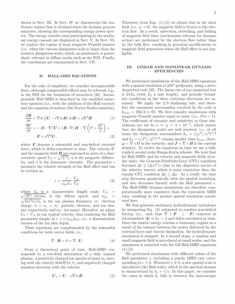
arXiv:1005.5422v1 [astro-ph.CO] 29 May 2010 Hall-MHD small-scale dynamos Daniel O. G´ omez, * Pablo D. Mininni, † and Pablo Dmitruk ‡ Departamento de F´ ısica, Facultad de Ciencias Exactas y Naturales, Universidad de Buenos Aires and CONICET, Ciudad Universitaria, 1428 Buenos Aires, Argentina. (Dated: June 1, 2010) Much of the progress in our understanding of dynamo mechanisms has been made within the theoretical framework of magnetohydrodynamics (MHD). However, for sufficiently diffuse media, the Hall effect eventually becomes non-negligible. We present results from three dimensional simulations of the Hall-MHD equations subjected to random non-helical forcing. We study the role of the Hall effect in the dynamo efficiency for different values of the Hall parameter, using a pseudospectral code to achieve exponentially fast convergence. We also study energy transfer rates among spatial scales to determine the relative importance of the various nonlinear effects in the dynamo process and in the energy cascade. The Hall effect produces a reduction of the direct energy cascade at scales larger than the Hall scale, and therefore leads to smaller energy dissipation rates. Finally, we present results stemming from simulations at large magnetic Prandtl numbers, which is the relevant regime in hot and diffuse media such a the interstellar medium. I. INTRODUCTION The generation of magnetic fields by dynamo activity plays an important role in a wide range of astrophysical objects, ranging from stars to clusters of galaxies. The gas in these objects is characterized by turbulent flows, as shown for instance by scintillation observations of the in- terstellar medium [1, 2], or from pressure maps in galaxy clusters [3]. Mechanisms able to generate magnetic fields by dynamo action are often classified as large- and small- scale dynamos, depending on the correlation length of the induced magnetic field. In this context, large and small are referred to the energy containing scale of the turbu- lent hydrodynamic flow. This classification is not rigid, as in many astrophysical objects both dynamos may be at work, but it gives a useful framework considering the limitations in the scale separation that can be achieved in numerical simulations. Also, the physical properties of the flows that can give rise to one or the other are somewhat different. Helical flows have proved efficient in generating large- scale dynamos, i.e., on scales larger than the energy- containing eddies of the flow [4–7]. It is now known that large-scale dynamo action can also be produced by anisotropic and inhomogeneous flows (e.g., flows with a large scale shear). On the other hand, non-helical flows can be instrumental in generating small-scale dy- namos [8], i.e., on sizes smaller than those of the energy- containing eddies [9–11]. In recent years, the study * [email protected]; http://astro.df.uba.ar; also at Instituto de Astronom´ ıa y F´ ısica del Espacio, C.C. 67 Suc. 28, 1428 Buenos Aires, Argentina. † also at IFIBA (Instituto de F´ ısica de Buenos Aires), CONICET, 1428 Buenos Aires, Argentina; and at National Center for Atmo- spheric Research, Boulder, CO 80307, USA. The National Center for Atmospheric Research is sponsored by the National Science Foundation. ‡ also at IFIBA (Instituto de F´ ısica de Buenos Aires), CONICET, 1428 Buenos Aires, Argentina. of small-scale dynamos with magnetic Prandtl number Pm = ν/η (the ratio between the viscosity and the mag- netic diffusivity of the plasma) different from unity has received special attention [12, 13], both for Pm ≫ 1 [14] and for Pm ≪ 1 [15, 16]. Motivations to study these regimes include recent experiments of dynamo action us- ing liquid sodium [17], as well as the fact that many astro- physical plasmas are characterized by magnetic Prandtl numbers different from unity. For instance, the magnetic Prandtl number is much smaller than one in the solar convective region, and it is typically much larger than one in the interplanetary medium and also in the inter- stellar medium (ISM). For sufficiently low-density media such as the one that pervades the ISM, kinetic effects such as the Hall effect or ambipolar diffusion might also become relevant [18]. The potential relevance of ambipolar diffusion in astrophysi- cal dynamos was studied in Refs. [19, 20]. The relevance of the Hall effect has been recognized in various astro- physical applications [18, 21, 22], space plasmas [23–25], and also laboratory plasmas [26–28]. The role of the Hall effect on large-scale dynamos subjected to helical forcing has also been addressed in the literature [29, 30]. Less attention has received the impact of kinetic effects on the small-scale dynamo. A theoretical model of the kine- matic small-scale dynamo with Hall effect was presented in [31], but to the best of our knowledge no numerical studies of the non-linear and saturated regime were con- sidered in the literature. In this paper, we present results from three dimen- sional simulations of the Hall-MHD equations subjected to random non-helical forcing. The main aim is to study the role of the Hall effect in the small-scale dynamo ef- ficiency for different values of the Hall parameter. As a result of the study, we also discuss the impact of the Hall effect on the dynamo saturation values, and on magnetic and total dissipation rates. The structure of the paper is as follows. A brief introduction to the theoretical frame- work known as Hall-MHD is presented in Sect. II. The role of the Hall effect in the efficiency of the dynamo is
-
Upload
independent -
Category
Documents
-
view
1 -
download
0
Transcript of Numerical simulations of Hall MHD small-scale dynamos
arX
iv:1
005.
5422
v1 [
astr
o-ph
.CO
] 2
9 M
ay 2
010
Hall-MHD small-scale dynamos
Daniel O. Gomez,∗ Pablo D. Mininni,† and Pablo Dmitruk‡
Departamento de Fısica, Facultad de Ciencias Exactas y Naturales,
Universidad de Buenos Aires and CONICET, Ciudad Universitaria, 1428 Buenos Aires, Argentina.
(Dated: June 1, 2010)
Much of the progress in our understanding of dynamo mechanisms has been made within thetheoretical framework of magnetohydrodynamics (MHD). However, for sufficiently diffuse media, theHall effect eventually becomes non-negligible. We present results from three dimensional simulationsof the Hall-MHD equations subjected to random non-helical forcing. We study the role of the Halleffect in the dynamo efficiency for different values of the Hall parameter, using a pseudospectralcode to achieve exponentially fast convergence. We also study energy transfer rates among spatialscales to determine the relative importance of the various nonlinear effects in the dynamo processand in the energy cascade. The Hall effect produces a reduction of the direct energy cascade atscales larger than the Hall scale, and therefore leads to smaller energy dissipation rates. Finally, wepresent results stemming from simulations at large magnetic Prandtl numbers, which is the relevantregime in hot and diffuse media such a the interstellar medium.
I. INTRODUCTION
The generation of magnetic fields by dynamo activityplays an important role in a wide range of astrophysicalobjects, ranging from stars to clusters of galaxies. Thegas in these objects is characterized by turbulent flows, asshown for instance by scintillation observations of the in-terstellar medium [1, 2], or from pressure maps in galaxyclusters [3]. Mechanisms able to generate magnetic fieldsby dynamo action are often classified as large- and small-scale dynamos, depending on the correlation length of theinduced magnetic field. In this context, large and smallare referred to the energy containing scale of the turbu-lent hydrodynamic flow. This classification is not rigid,as in many astrophysical objects both dynamos may beat work, but it gives a useful framework considering thelimitations in the scale separation that can be achievedin numerical simulations. Also, the physical propertiesof the flows that can give rise to one or the other aresomewhat different.Helical flows have proved efficient in generating large-
scale dynamos, i.e., on scales larger than the energy-containing eddies of the flow [4–7]. It is now knownthat large-scale dynamo action can also be produced byanisotropic and inhomogeneous flows (e.g., flows witha large scale shear). On the other hand, non-helicalflows can be instrumental in generating small-scale dy-namos [8], i.e., on sizes smaller than those of the energy-containing eddies [9–11]. In recent years, the study
∗ [email protected]; http://astro.df.uba.ar; also at Instituto deAstronomıa y Fısica del Espacio, C.C. 67 Suc. 28, 1428 BuenosAires, Argentina.
† also at IFIBA (Instituto de Fısica de Buenos Aires), CONICET,1428 Buenos Aires, Argentina; and at National Center for Atmo-spheric Research, Boulder, CO 80307, USA. The National Centerfor Atmospheric Research is sponsored by the National ScienceFoundation.
‡ also at IFIBA (Instituto de Fısica de Buenos Aires), CONICET,1428 Buenos Aires, Argentina.
of small-scale dynamos with magnetic Prandtl numberPm = ν/η (the ratio between the viscosity and the mag-netic diffusivity of the plasma) different from unity hasreceived special attention [12, 13], both for Pm ≫ 1 [14]and for Pm ≪ 1 [15, 16]. Motivations to study theseregimes include recent experiments of dynamo action us-ing liquid sodium [17], as well as the fact that many astro-physical plasmas are characterized by magnetic Prandtlnumbers different from unity. For instance, the magneticPrandtl number is much smaller than one in the solarconvective region, and it is typically much larger thanone in the interplanetary medium and also in the inter-stellar medium (ISM).
For sufficiently low-density media such as the one thatpervades the ISM, kinetic effects such as the Hall effect orambipolar diffusion might also become relevant [18]. Thepotential relevance of ambipolar diffusion in astrophysi-cal dynamos was studied in Refs. [19, 20]. The relevanceof the Hall effect has been recognized in various astro-physical applications [18, 21, 22], space plasmas [23–25],and also laboratory plasmas [26–28]. The role of the Halleffect on large-scale dynamos subjected to helical forcinghas also been addressed in the literature [29, 30]. Lessattention has received the impact of kinetic effects onthe small-scale dynamo. A theoretical model of the kine-matic small-scale dynamo with Hall effect was presentedin [31], but to the best of our knowledge no numericalstudies of the non-linear and saturated regime were con-sidered in the literature.
In this paper, we present results from three dimen-sional simulations of the Hall-MHD equations subjectedto random non-helical forcing. The main aim is to studythe role of the Hall effect in the small-scale dynamo ef-ficiency for different values of the Hall parameter. As aresult of the study, we also discuss the impact of the Halleffect on the dynamo saturation values, and on magneticand total dissipation rates. The structure of the paper isas follows. A brief introduction to the theoretical frame-work known as Hall-MHD is presented in Sect. II. Therole of the Hall effect in the efficiency of the dynamo is
2
shown in Sect. III. In Sect. IV we characterize the sta-tionary regime that is attained when the dynamo processsaturates, showing the corresponding energy power spec-tra. The energy transfer rates participating in the nonlin-ear energy cascade are displayed in Sect. V. In Sect. VI,we explore the regime of large magnetic Prandtl number(i.e., when the viscous dissipation scale is larger than theresistive dissipation scale) which, as mentioned, is partic-ularly relevant in diffuse media such as the ISM. Finally,the conclusions are summarized in Sect. VII.
II. HALL-MHD EQUATIONS
For the sake of simplicity, we consider incompressibleflows, although compressible effects may be relevant, e.g.,in the ISM for the formation of structures [32]. Incom-pressible Hall-MHD is described by the modified induc-tion equation (i.e., with the addition of the Hall current)and the equation of motion (the Navier-Stokes equation),
∂B
∂t= ∇× [(U − ǫ∇×B)×B] + η∇2B (1)
∂U
∂t= − (U · ∇)U + (B · ∇)B −∇
(
P +B2
2
)
+
F + ν∇2U , (2)
where F denotes a solenoidal and non-helical externalforce, which is delta-correlated in time. The velocity U
and the magnetic field B are expressed in units of a char-acteristic speed U0 =
√
〈U2〉; η is the magnetic diffusiv-ity, and ν is the kinematic viscosity. The parameter ǫmeasures the relative strength of the Hall effect and canbe written as
ǫ =c
ωpiL0
UA
U0
, (3)
where L0 is a characteristic length scale, UA =√
〈B2〉 /4πnmi is the Alfven speed, and wpi =√
4πe2n/mi is the ion plasma frequency (e: electroncharge, n = ne = ni: particle, electron, and ion den-sity respectively, and mi: ion mass). Hereafter, we adoptU0 = UA as our typical velocity, thus rendering the Hallparameter simply as ǫ = c/(ωpiL0), i.e., a dimensionlessversion of the ion skin depth.These equations are complemented by the solenoidal
conditions for both vector fields, i.e.,
∇ ·B = 0 = ∇ ·U . (4)
From a theoretical point of view, Hall-MHD cor-responds to a two-fluid description of a fully ionizedplasma: a positively charged ion species of mass mi mov-ing with the velocity field U(r, t), and negatively chargedmassless electrons with the velocity
U e = U − ǫ∇×B. (5)
Therefore, from Eqs. (1)-(5) we obtain that in the ideallimit (i.e. η → 0), the magnetic field is frozen to the elec-tron flow. As a result, advection, stretching, and foldingof magnetic field lines (mechanisms relevant for dynamoaction) are performed by the electron flow rather thanby the bulk flow, resulting in potential modifications tomagnetic field generation when the Hall effect is not neg-ligible.
III. LINEAR AND NONLINEAR DYNAMO
EFFICIENCIES
We performed simulations of the Hall-MHD equationswith a spatial resolution of 2563 gridpoints, using a pseu-dospectral code [33]. The linear size of our numerical boxis 2πL0 (with L0 a unit length), and periodic bound-ary conditions in the three cartesian directions are as-sumed. We apply the 2/3 dealiasing rule, and there-fore the maximum wavenumber resolved by the code iskmax = 256/3 ≈ 85. We first consider simulations withmagnetic Prandtl number equal to unity (i.e., Pm = 1).The coefficients of viscosity and resistivity in these sim-ulations are set to ν = η = 2 × 10⁻³, which ensurethat the dissipation scales are well resolved, i.e., at alltimes the dissipation wavenumbers kν = (
⟨ω2
⟩/ν2)1/4
and kη = (⟨J2
⟩/η2)1/4 remain smaller than kmax (here,
ω = ∇×U is the vorticity, and J = ∇×B is the currentdensity). To evolve the equations in time we use a fullyexplicit second order Runge-Kutta scheme. We note thatfor Hall-MHD, and for velocity and magnetic fields of or-der unity, the Courant-Friedrichs-Levy (CFL) conditionbecomes ∆t ≤ (∆x)2/ǫ (due to the dispersive nature ofthe whistler waves), which is more restrictive than theregular CFL condition ∆t ≤ ∆x. As a result, the timestep decreases quadratically with the spatial resolution,and also decreases linearly with the Hall parameter ǫ.The Hall-MHD dynamo simulations are therefore com-putationally more expensive than the equivalent MHDruns, resulting in the modest spatial resolution consid-ered here.We first generate stationary hydrodynamic turbulence
by integrating Eq. (2) subjected to random non-helicalforcing (i.e., such that ∇ × F ⊥ F ) centered atwavenumbers |k| ≈ kF = 3 and delta-correlated in time.Once the kinetic energy reaches a stationary regime as aresult of the balance between the power delivered by theexternal force and viscous dissipation, the hydrodynamicsimulation is stopped. In a second stage, a random andsmall magnetic field is introduced at small scales, and thesimulation is restarted with the full Hall-MHD equations(1)-(2).We performed simulations with different values of the
Hall parameter ǫ, including a purely MHD case corre-sponding to ǫ = 0. Whenever ǫ 6= 0, a new spatial scale isintroduced (the Hall scale), which in the spectral domainis characterized by kǫ = 1/ǫ. In this paper, we considerthe cases in which kǫ falls in between the macroscopic

3
FIG. 1. Kinetic (thin) and magnetic (thick) energies vs. timefor ǫ = 0, 0.05, and 0.10 (from top to bottom).
FIG. 2. Kinetic (thin) and magnetic (thick) dissipation ratesvs. time for ǫ = 0, 0.05, and 0.10 (from top to bottom).
scale kF (set by the external driver) and the dissipationscales kν and kη, which is the relevant scenario for as-trophysical plasmas such as the interstellar medium. Insuch media, the Hall scale is several orders of magnitudesmaller than the largest scales, and the Hall effect canbe expected to be relevant only at the smallest dynam-ical scales. Note, however, that these arguments oughtto be regarded as motivations. Although the ordering oftypical length scales is the correct one, a realistic sepa-ration of scales is completely out of reach with presentcomputing power.
In Fig. 1 we show the statistically stationary time se-ries for kinetic energy (thin lines) for runs with differentvalues of the Hall parameter ǫ. The magnetic energy inthese runs (thick line) is observed to rise until it satu-rates at values which remain a moderate fraction of thecorresponding kinetic energy. The viscous (thin line) andresistive (thick) dissipation rates vs. time are shown inFig. 2 for three runs with different values of the Hall pa-rameter. In all these plots, the magnetic dissipation rateis observed to grow until it becomes fully comparableto the corresponding viscous dissipation rate (even whenthe kinetic energy is larger than the magnetic energy).
The exponentially fast growth of magnetic energy isshown using a lin-log scale in Fig. 3 for the same threeruns. Note that there is an initial stage where the mag-netic field starts growing exponentially fast, regardless ofthe particular value of the Hall parameter ǫ. During thisearly stage of the dynamo, the electron flow is still ap-
FIG. 3. Magnetic energy vs. time, showing the exponentialgrowth rate during the early linear dynamo regime.
proximately equal to the ion flow, i.e. Ue ≈ U [see Eq.(5)]. Keeping in mind that the growing magnetic fieldremains approximately frozen (note that this is strictlyvalid only in the limit η → 0) to the electron velocityfield, we can anticipate that at some point in time theelectron and ion flows will start drifting appart from oneanother. Therefore, a second stage arises correspondingto a non-linear dynamo (although still “kinematic,” inthe sense that the magnetic field does not affect the bulkvelocity field), since the magnetic field is being advectedby the electron flow which at that point becomes a func-tion of the magnetic field itself. In Fig. 3 we see thatalthough the case ǫ = 0 can be approximated by a lineargrowth rate (indicated by the dotted straight line) all theway up to the saturation level, we cannot do the samefor the cases ǫ = 0.05, and 0.10 since there is a break inthe corresponding growth rates. This break occurs firstfor the case with larger Hall effect (i.e., ǫ = 0.10), butthe incremented slope is larger for the case ǫ = 0.05. Thefact that the dynamo efficiency improves up to a certainvalue of the Hall parameter and then starts decreasing,is reminiscent of similar results reported in Ref. [33] forlarge-scale Hall-MHD dynamos.To show the relative importance of the Hall term in
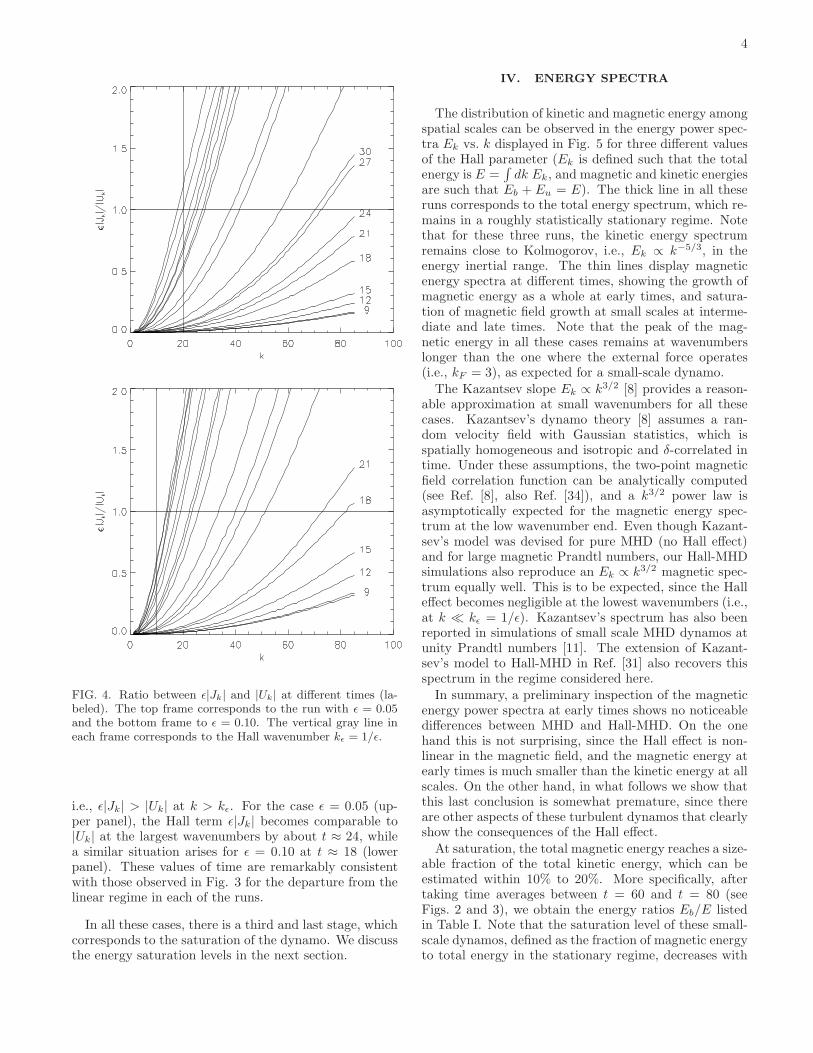
the electron velocity field, in Fig. 4 we display the ratiobetween ǫ|Jk| and |Uk| at different labeled times, where|Jk| and |Uk| are respectively the spectral intensities ofthe current density and of the velocity field at wavenum-ber k [note that U e = U − ǫJ from Eq. (5)]. The upperframe corresponds to the run with ǫ = 0.05 and the lowerframe to ǫ = 0.10. The vertical gray line in each framecorresponds to the Hall scale kǫ = 1/ǫ. In both cases, theHall term becomes gradually non-negligible and eventu-ally dominant at the largest wavenumbers of the system,
4
FIG. 4. Ratio between ǫ|Jk| and |Uk| at different times (la-beled). The top frame corresponds to the run with ǫ = 0.05and the bottom frame to ǫ = 0.10. The vertical gray line ineach frame corresponds to the Hall wavenumber kǫ = 1/ǫ.
i.e., ǫ|Jk| > |Uk| at k > kǫ. For the case ǫ = 0.05 (up-per panel), the Hall term ǫ|Jk| becomes comparable to|Uk| at the largest wavenumbers by about t ≈ 24, whilea similar situation arises for ǫ = 0.10 at t ≈ 18 (lowerpanel). These values of time are remarkably consistentwith those observed in Fig. 3 for the departure from thelinear regime in each of the runs.
In all these cases, there is a third and last stage, whichcorresponds to the saturation of the dynamo. We discussthe energy saturation levels in the next section.
IV. ENERGY SPECTRA
The distribution of kinetic and magnetic energy amongspatial scales can be observed in the energy power spec-tra Ek vs. k displayed in Fig. 5 for three different valuesof the Hall parameter (Ek is defined such that the totalenergy is E =
∫dk Ek, and magnetic and kinetic energies
are such that Eb + Eu = E). The thick line in all theseruns corresponds to the total energy spectrum, which re-mains in a roughly statistically stationary regime. Notethat for these three runs, the kinetic energy spectrumremains close to Kolmogorov, i.e., Ek ∝ k−5/3, in theenergy inertial range. The thin lines display magneticenergy spectra at different times, showing the growth ofmagnetic energy as a whole at early times, and satura-tion of magnetic field growth at small scales at interme-diate and late times. Note that the peak of the mag-netic energy in all these cases remains at wavenumberslonger than the one where the external force operates(i.e., kF = 3), as expected for a small-scale dynamo.
The Kazantsev slope Ek ∝ k3/2 [8] provides a reason-able approximation at small wavenumbers for all thesecases. Kazantsev’s dynamo theory [8] assumes a ran-dom velocity field with Gaussian statistics, which isspatially homogeneous and isotropic and δ-correlated intime. Under these assumptions, the two-point magneticfield correlation function can be analytically computed(see Ref. [8], also Ref. [34]), and a k3/2 power law isasymptotically expected for the magnetic energy spec-trum at the low wavenumber end. Even though Kazant-sev’s model was devised for pure MHD (no Hall effect)and for large magnetic Prandtl numbers, our Hall-MHDsimulations also reproduce an Ek ∝ k3/2 magnetic spec-trum equally well. This is to be expected, since the Halleffect becomes negligible at the lowest wavenumbers (i.e.,at k ≪ kǫ = 1/ǫ). Kazantsev’s spectrum has also beenreported in simulations of small scale MHD dynamos atunity Prandtl numbers [11]. The extension of Kazant-sev’s model to Hall-MHD in Ref. [31] also recovers thisspectrum in the regime considered here.In summary, a preliminary inspection of the magnetic
energy power spectra at early times shows no noticeabledifferences between MHD and Hall-MHD. On the onehand this is not surprising, since the Hall effect is non-linear in the magnetic field, and the magnetic energy atearly times is much smaller than the kinetic energy at allscales. On the other hand, in what follows we show thatthis last conclusion is somewhat premature, since thereare other aspects of these turbulent dynamos that clearlyshow the consequences of the Hall effect.
At saturation, the total magnetic energy reaches a size-able fraction of the total kinetic energy, which can beestimated within 10% to 20%. More specifically, aftertaking time averages between t = 60 and t = 80 (seeFigs. 2 and 3), we obtain the energy ratios Eb/E listedin Table I. Note that the saturation level of these small-scale dynamos, defined as the fraction of magnetic energyto total energy in the stationary regime, decreases with

5
TABLE I. Global results for runs with different values of theHall parameter ǫ. E is the mean saturation level of the totalenergy, Eb/E is the ratio of magnetic to total energy, kJ is theaverage wavenumber for the current density distribution, D isthe total dissipation rate, and Db/D is the ratio of magneticto total dissipation rate.
ǫ E Eb/E kJ D Db/D
0.00 0.37 0.14 23.1 0.13 0.48
0.05 0.35 0.13 19.4 0.11 0.39
0.10 0.33 0.13 17.4 0.10 0.34
the Hall parameter. Therefore, although in the lineardynamo regime the growth rate increases with the Hallparameter ǫ, the magnetic field reaches a smaller satura-tion level.As mentioned in Sect. III, the dynamics of the largest
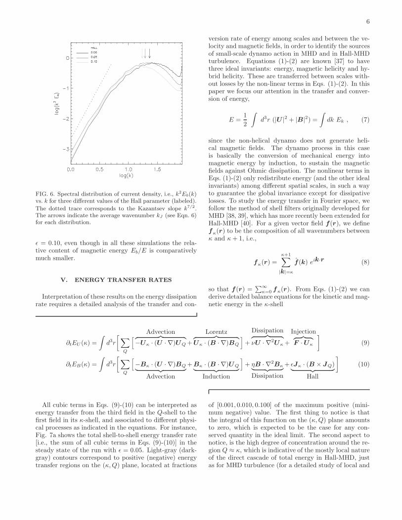
wavenumbers in our simulations is controlled by viscosityand electric resistivity. Therefore, the dissipation of mag-netic energy mostly takes place in current sheets with athickness which can be expected to be close to the in-verse of kη ≈ 85. On the other hand, the width andthe length of these current sheets will vary from oneto another [13, 35]. We can obtain a statistical aver-age of the dimensions of our magnetic dissipative struc-tures by computing the power spectrum of the electriccurrent density, which is simply k2Eb(k). In Fig. 6 weshow time averaged (between t = 60 and t = 80) cur-rent density spectra for three different values of the Hallparameter (labeled). All of these spectra are compat-ible with a Kazantsev law at low wavenumbers. Notethat the maximum of these spectra shift toward smallerwavenumbers as the Hall parameter increases. Since thepeak of the spectrum can be associated to an averagethickness of the current sheets, the above mentioned shiftcan be interpreted as the current sheets becoming rela-tively “thicker” as the Hall effect increases. This result isin agreement with previous experimental and numericalresults suggesting that in Hall-MHD the thickness of thecurrent sheets is given by the Hall scale rather than bythe Ohmic dissipative scale as in the MHD case (see [36]for recent results in support of this interpretation).For each of these runs, we also compute the magnetic
Taylor wavenumber kJ given by
k2J =
∫dk k2 Eb(k)∫dk Eb(k)
(6)
which are indicated in Figure 6 by arrows, and are ob-served to remain close, but somewhat to the left of themaximum for the corresponding power spectrum. Themagnetic Taylor scale (i.e., the inverse of kJ) can be in-terpreted as the mean curvature of the magnetic fieldlines [13] and of the ensuing current sheets. The value ofkJ also moves towards smaller wavenumbers as the Hallscale is increased. The values of kJ for each of these runs
FIG. 5. Total energy spectrum (thick trace) at t = 72 fordifferent values of ǫ (labeled). In each frame magnetic energyspectra at t = 18, 36, 72 are also shown (corresponding tothe thin lines from bottom to top). The Kolmogorov andKazantsev spectra are overlaid (dotted trace) for reference.
are listed in Table I. In Table I we also list the timeaveraged total dissipation rate D = Du + Db, clearlyshowing a progressive reduction as the Hall parameteris increased. The ratio of magnetic to total dissipationDb/D also reduces as ǫ increases, going from approxi-mate equipartition in the MHD case to about 33% for
6
FIG. 6. Spectral distribution of current density, i.e., k2Eb(k)vs. k for three different values of the Hall parameter (labeled).
The dotted trace corresponds to the Kazantsev slope k7/2.The arrows indicate the average wavenumber kJ (see Eqn. 6)for each distribution.
ǫ = 0.10, even though in all these simulations the rela-tive content of magnetic energy Eb/E is comparativelymuch smaller.
V. ENERGY TRANSFER RATES
Interpretation of these results on the energy dissipationrate requires a detailed analysis of the transfer and con-
version rate of energy among scales and between the ve-locity and magnetic fields, in order to identify the sourcesof small-scale dynamo action in MHD and in Hall-MHDturbulence. Equations (1)-(2) are known [37] to havethree ideal invariants: energy, magnetic helicity and hy-brid helicity. These are transferred between scales with-out losses by the non-linear terms in Eqs. (1)-(2). In thispaper we focus our attention in the transfer and conver-sion of energy,
E =1
2
∫
d3r (|U |2 + |B|2) =
∫
dk Ek , (7)
since the non-helical dynamo does not generate heli-cal magnetic fields. The dynamo process in this caseis basically the conversion of mechanical energy intomagnetic energy by induction, to sustain the magneticfields against Ohmic dissipation. The nonlinear terms inEqs. (1)-(2) only redistribute energy (and the other idealinvariants) among different spatial scales, in such a wayto guarantee the global invariance except for dissipativelosses. To study the energy transfer in Fourier space, wefollow the method of shell filters originally developed forMHD [38, 39], which has more recently been extended forHall-MHD [40]. For a given vector field f(r), we definefκ(r) to be the composition of all wavenumbers betweenκ and κ+ 1, i.e.,
fκ(r) =κ+1∑
|k|=κ
f(k) eik·r (8)
so that f (r) =∑∞
κ=0fκ(r). From Eqs. (1)-(2) we can
derive detailed balance equations for the kinetic and mag-netic energy in the κ-shell
∂tEU (κ) =
∫
d3r
[∑
Q
[Advection
︷ ︸︸ ︷
−Uκ · (U · ∇)UQ +
Lorentz︷ ︸︸ ︷
Uκ · (B · ∇)BQ
]
+
Dissipation︷ ︸︸ ︷
νU · ∇2Uκ +
Injection︷ ︸︸ ︷
F ·Uκ
]
(9)
∂tEB(κ) =
∫
d3r
[∑
Q
[
−Bκ · (U · ∇)BQ︸ ︷︷ ︸
Advection
+Bκ · (B · ∇)UQ︸ ︷︷ ︸
Induction
]
+ ηB · ∇2Bκ︸ ︷︷ ︸
Dissipation
+ ǫJκ · (B × JQ)︸ ︷︷ ︸
Hall
]
(10)
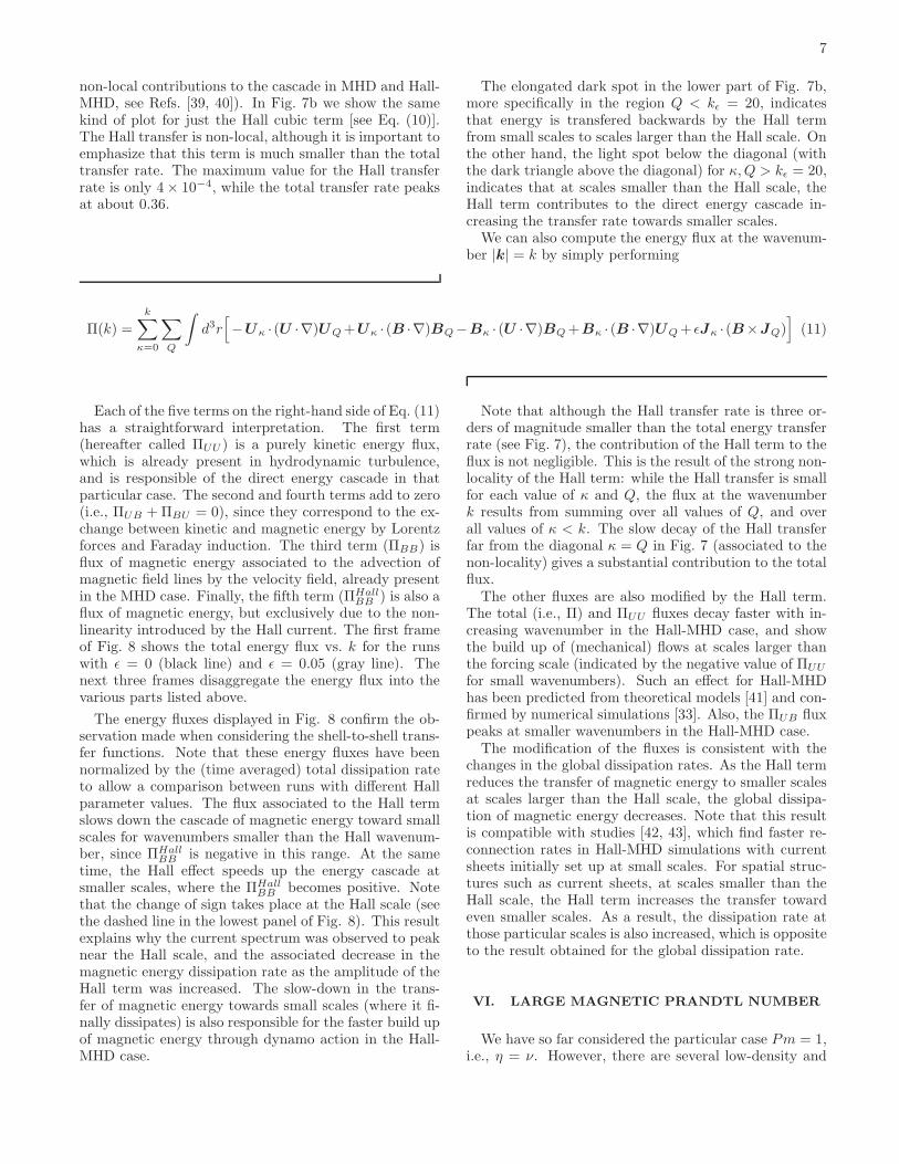
All cubic terms in Eqs. (9)-(10) can be interpreted asenergy transfer from the third field in the Q-shell to thefirst field in its κ-shell, and associated to different physi-cal processes as indicated in the equations. For instance,Fig. 7a shows the total shell-to-shell energy transfer rate[i.e., the sum of all cubic terms in Eqs. (9)-(10)] in thesteady state of the run with ǫ = 0.05. Light-gray (dark-gray) contours correspond to positive (negative) energytransfer regions on the (κ,Q) plane, located at fractions
of [0.001, 0.010, 0.100] of the maximum positive (mini-mum negative) value. The first thing to notice is thatthe integral of this function on the (κ,Q) plane amountsto zero, which is expected to be the case for any con-served quantity in the ideal limit. The second aspect tonotice, is the high degree of concentration around the re-gion Q ≈ κ, which is indicative of the mostly local natureof the direct cascade of total energy in Hall-MHD, justas for MHD turbulence (for a detailed study of local and
7
non-local contributions to the cascade in MHD and Hall-MHD, see Refs. [39, 40]). In Fig. 7b we show the samekind of plot for just the Hall cubic term [see Eq. (10)].The Hall transfer is non-local, although it is important toemphasize that this term is much smaller than the totaltransfer rate. The maximum value for the Hall transferrate is only 4× 10⁻⁴, while the total transfer rate peaksat about 0.36.
The elongated dark spot in the lower part of Fig. 7b,more specifically in the region Q < kǫ = 20, indicatesthat energy is transfered backwards by the Hall termfrom small scales to scales larger than the Hall scale. Onthe other hand, the light spot below the diagonal (withthe dark triangle above the diagonal) for κ,Q > kǫ = 20,indicates that at scales smaller than the Hall scale, theHall term contributes to the direct energy cascade in-creasing the transfer rate towards smaller scales.We can also compute the energy flux at the wavenum-
ber |k| = k by simply performing
Π(k) =
k∑
κ=0
∑
Q
∫
d3r[
−Uκ · (U ·∇)UQ+Uκ · (B ·∇)BQ−Bκ · (U ·∇)BQ+Bκ · (B ·∇)UQ+ ǫJκ · (B×JQ)]
(11)
Each of the five terms on the right-hand side of Eq. (11)has a straightforward interpretation. The first term(hereafter called ΠUU ) is a purely kinetic energy flux,which is already present in hydrodynamic turbulence,and is responsible of the direct energy cascade in thatparticular case. The second and fourth terms add to zero(i.e., ΠUB +ΠBU = 0), since they correspond to the ex-change between kinetic and magnetic energy by Lorentzforces and Faraday induction. The third term (ΠBB) isflux of magnetic energy associated to the advection ofmagnetic field lines by the velocity field, already presentin the MHD case. Finally, the fifth term (ΠHall
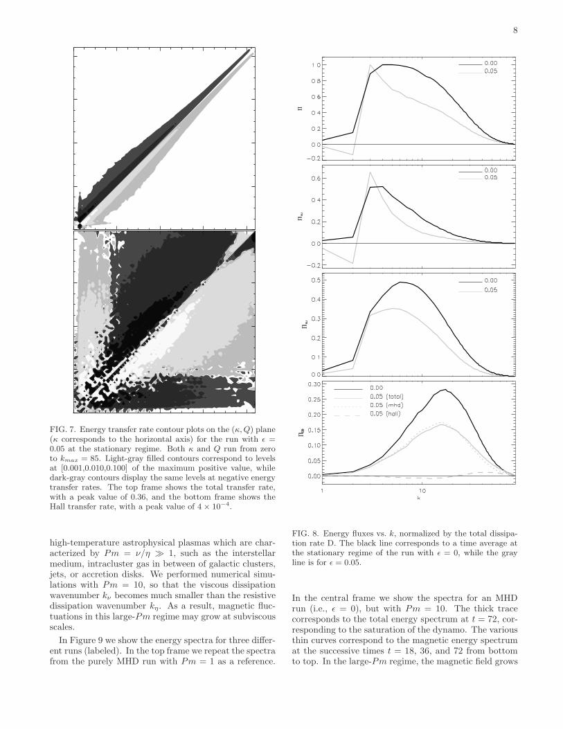
BB ) is also aflux of magnetic energy, but exclusively due to the non-linearity introduced by the Hall current. The first frameof Fig. 8 shows the total energy flux vs. k for the runswith ǫ = 0 (black line) and ǫ = 0.05 (gray line). Thenext three frames disaggregate the energy flux into thevarious parts listed above.
The energy fluxes displayed in Fig. 8 confirm the ob-servation made when considering the shell-to-shell trans-fer functions. Note that these energy fluxes have beennormalized by the (time averaged) total dissipation rateto allow a comparison between runs with different Hallparameter values. The flux associated to the Hall termslows down the cascade of magnetic energy toward smallscales for wavenumbers smaller than the Hall wavenum-ber, since ΠHall
BB is negative in this range. At the sametime, the Hall effect speeds up the energy cascade atsmaller scales, where the ΠHall
BB becomes positive. Notethat the change of sign takes place at the Hall scale (seethe dashed line in the lowest panel of Fig. 8). This resultexplains why the current spectrum was observed to peaknear the Hall scale, and the associated decrease in themagnetic energy dissipation rate as the amplitude of theHall term was increased. The slow-down in the trans-fer of magnetic energy towards small scales (where it fi-nally dissipates) is also responsible for the faster build upof magnetic energy through dynamo action in the Hall-MHD case.
Note that although the Hall transfer rate is three or-ders of magnitude smaller than the total energy transferrate (see Fig. 7), the contribution of the Hall term to theflux is not negligible. This is the result of the strong non-locality of the Hall term: while the Hall transfer is smallfor each value of κ and Q, the flux at the wavenumberk results from summing over all values of Q, and overall values of κ < k. The slow decay of the Hall transferfar from the diagonal κ = Q in Fig. 7 (associated to thenon-locality) gives a substantial contribution to the totalflux.The other fluxes are also modified by the Hall term.
The total (i.e., Π) and ΠUU fluxes decay faster with in-creasing wavenumber in the Hall-MHD case, and showthe build up of (mechanical) flows at scales larger thanthe forcing scale (indicated by the negative value of ΠUU
for small wavenumbers). Such an effect for Hall-MHDhas been predicted from theoretical models [41] and con-firmed by numerical simulations [33]. Also, the ΠUB fluxpeaks at smaller wavenumbers in the Hall-MHD case.The modification of the fluxes is consistent with the
changes in the global dissipation rates. As the Hall termreduces the transfer of magnetic energy to smaller scalesat scales larger than the Hall scale, the global dissipa-tion of magnetic energy decreases. Note that this resultis compatible with studies [42, 43], which find faster re-connection rates in Hall-MHD simulations with currentsheets initially set up at small scales. For spatial struc-tures such as current sheets, at scales smaller than theHall scale, the Hall term increases the transfer towardeven smaller scales. As a result, the dissipation rate atthose particular scales is also increased, which is oppositeto the result obtained for the global dissipation rate.
VI. LARGE MAGNETIC PRANDTL NUMBER
We have so far considered the particular case Pm = 1,i.e., η = ν. However, there are several low-density and
8
FIG. 7. Energy transfer rate contour plots on the (κ,Q) plane(κ corresponds to the horizontal axis) for the run with ǫ =0.05 at the stationary regime. Both κ and Q run from zeroto kmax = 85. Light-gray filled contours correspond to levelsat [0.001,0.010,0.100] of the maximum positive value, whiledark-gray contours display the same levels at negative energytransfer rates. The top frame shows the total transfer rate,with a peak value of 0.36, and the bottom frame shows theHall transfer rate, with a peak value of 4× 10⁻⁴.
high-temperature astrophysical plasmas which are char-acterized by Pm = ν/η ≫ 1, such as the interstellarmedium, intracluster gas in between of galactic clusters,jets, or accretion disks. We performed numerical simu-lations with Pm = 10, so that the viscous dissipationwavenumber kν becomes much smaller than the resistivedissipation wavenumber kη. As a result, magnetic fluc-tuations in this large-Pm regime may grow at subviscousscales.
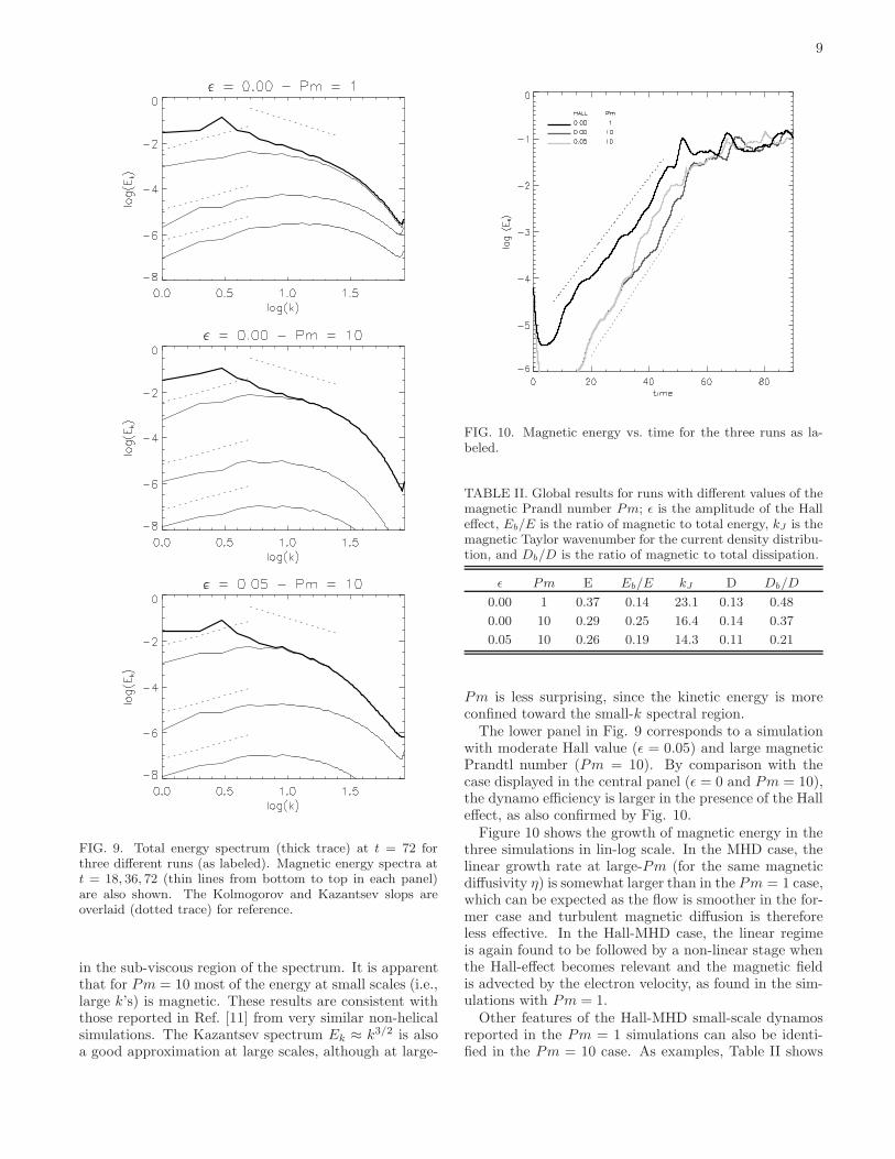
In Figure 9 we show the energy spectra for three differ-ent runs (labeled). In the top frame we repeat the spectrafrom the purely MHD run with Pm = 1 as a reference.
FIG. 8. Energy fluxes vs. k, normalized by the total dissipa-tion rate D. The black line corresponds to a time average atthe stationary regime of the run with ǫ = 0, while the grayline is for ǫ = 0.05.
In the central frame we show the spectra for an MHDrun (i.e., ǫ = 0), but with Pm = 10. The thick tracecorresponds to the total energy spectrum at t = 72, cor-responding to the saturation of the dynamo. The variousthin curves correspond to the magnetic energy spectrumat the successive times t = 18, 36, and 72 from bottomto top. In the large-Pm regime, the magnetic field grows
9
FIG. 9. Total energy spectrum (thick trace) at t = 72 forthree different runs (as labeled). Magnetic energy spectra att = 18, 36, 72 (thin lines from bottom to top in each panel)are also shown. The Kolmogorov and Kazantsev slops areoverlaid (dotted trace) for reference.
in the sub-viscous region of the spectrum. It is apparentthat for Pm = 10 most of the energy at small scales (i.e.,large k’s) is magnetic. These results are consistent withthose reported in Ref. [11] from very similar non-helicalsimulations. The Kazantsev spectrum Ek ≈ k3/2 is alsoa good approximation at large scales, although at large-
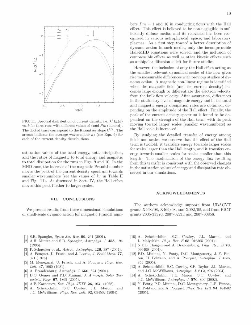
FIG. 10. Magnetic energy vs. time for the three runs as la-beled.
TABLE II. Global results for runs with different values of themagnetic Prandl number Pm; ǫ is the amplitude of the Halleffect, Eb/E is the ratio of magnetic to total energy, kJ is themagnetic Taylor wavenumber for the current density distribu-tion, and Db/D is the ratio of magnetic to total dissipation.
ǫ Pm E Eb/E kJ D Db/D
0.00 1 0.37 0.14 23.1 0.13 0.48
0.00 10 0.29 0.25 16.4 0.14 0.37
0.05 10 0.26 0.19 14.3 0.11 0.21
Pm is less surprising, since the kinetic energy is moreconfined toward the small-k spectral region.The lower panel in Fig. 9 corresponds to a simulation
with moderate Hall value (ǫ = 0.05) and large magneticPrandtl number (Pm = 10). By comparison with thecase displayed in the central panel (ǫ = 0 and Pm = 10),the dynamo efficiency is larger in the presence of the Halleffect, as also confirmed by Fig. 10.Figure 10 shows the growth of magnetic energy in the
three simulations in lin-log scale. In the MHD case, thelinear growth rate at large-Pm (for the same magneticdiffusivity η) is somewhat larger than in the Pm = 1 case,which can be expected as the flow is smoother in the for-mer case and turbulent magnetic diffusion is thereforeless effective. In the Hall-MHD case, the linear regimeis again found to be followed by a non-linear stage whenthe Hall-effect becomes relevant and the magnetic fieldis advected by the electron velocity, as found in the sim-ulations with Pm = 1.Other features of the Hall-MHD small-scale dynamos
reported in the Pm = 1 simulations can also be identi-fied in the Pm = 10 case. As examples, Table II shows
10
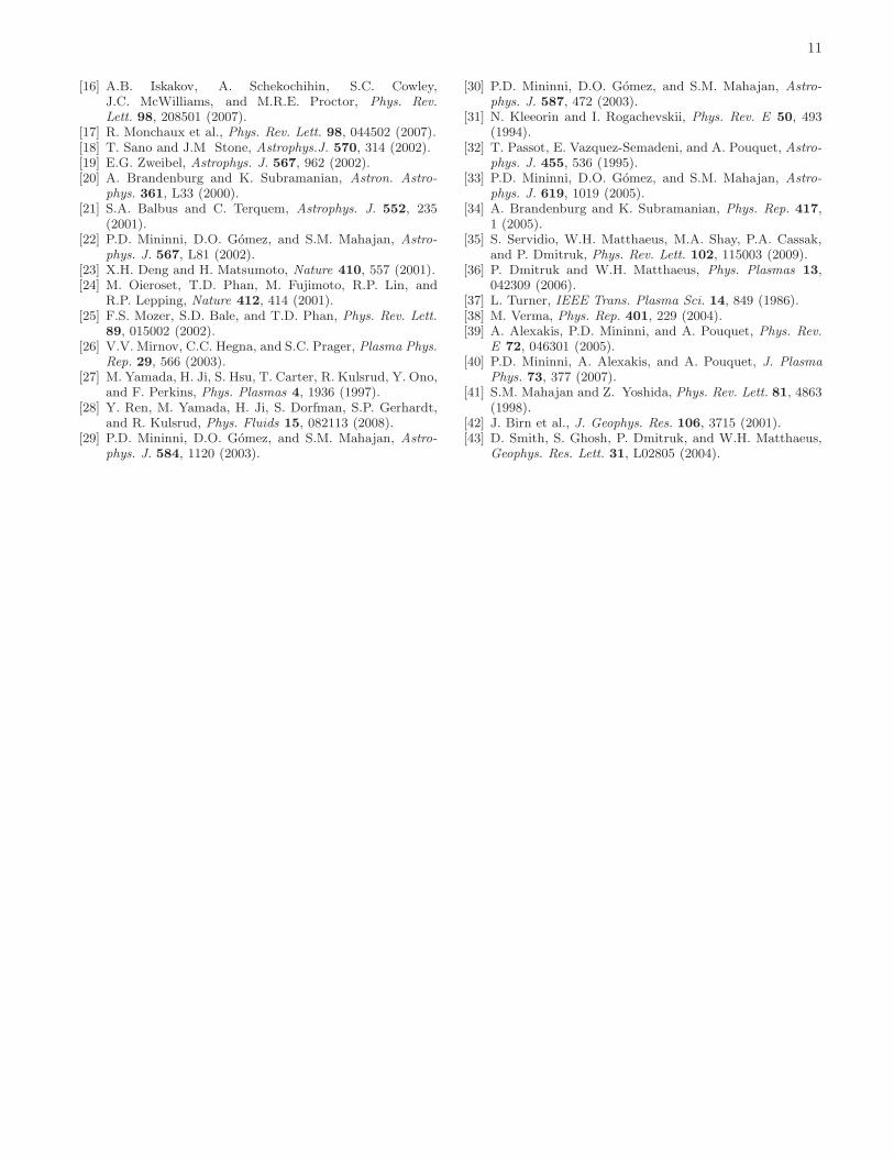
FIG. 11. Spectral distribution of current density, i.e. k2Eb(k)vs. k for three runs with different values of ǫ and Pm (labeled).
The dotted trace correspond to the Kazantsev slope k7/2. Thearrows indicate the average wavenumber kJ (see Eqn. 6) foreach of the current density distributions.
saturation values of the total energy, total dissipation,and the ratios of magnetic to total energy and magneticto total dissipation for the runs in Figs. 9 and 10. In theMHD case, the increase of the magnetic Prandtl numbermoves the peak of the current density spectrum towardssmaller wavenumbers (see the values of kJ in Table IIand Fig. 11). As discussed in Sect. IV, the Hall effectmoves this peak further to larger scales.
VII. CONCLUSIONS
We present results from three dimensional simulationsof small-scale dynamo action for magnetic Prandtl num-
bers Pm = 1 and 10 in conducting flows with the Halleffect. This effect is believed to be non-negligible in suf-ficiently diffuse media, and its relevance has been rec-ognized in various astrophysical, space, and laboratoryplasmas. As a first step toward a better description ofdynamo action in such media, only the incompressibleHall-MHD equations were solved, and the inclusion ofcompressible effects as well as other kinetic effects suchas ambipolar difussion is left for future studies.
However, the inclusion of only the Hall effect acting atthe smallest relevant dynamical scales of the flow givesrise to measurable differences with previous studies of dy-namo action. A magnetic non-linear regime is identifiedwhen the magnetic field (and the current density) be-comes large enough to differentiate the electron velocityfrom the bulk flow velocity. After saturation, differencesin the stationary level of magnetic energy and in the totaland magnetic energy dissipation rates are obtained, de-pending on the amplitude of the Hall effect. Finally, thepeak of the current density spectrum is found to be de-pendent on the strength of the Hall term, with its peakmoving toward larger scales (smaller wavenumbers) asthe Hall scale is increased.
By studying the detailed transfer of energy amongfields and scales, we observe that the effect of the Hallterm is twofold: it transfers energy towards larger scalesfor scales larger than the Hall length, and it transfers en-ergy towards smaller scales for scales smaller than thislength. The modification of the energy flux resultingfrom this transfer is consistent with the observed changesin the saturation values of energy and dissipation rate ob-served in our simulations.
ACKNOWLEDGMENTS
The authors acknowledge support from UBACYTgrants X468/08, X469/08, and X092/08, and from PICTgrants 2005-33370, 2007-02211 and 2007-00856.
[1] S.R. Spangler, Space Sci. Rev. 99, 261 (2001).[2] A.H. Minter and S.R. Spangler, Astrophys. J. 458, 194
(1996).[3] P. Schuecker et al., Astron. Astrophys. 426, 387 (2004).[4] A. Pouquet, U. Frisch, and J. Leorat, J. Fluid Mech. 77,
321 (1976).[5] M. Meneguzzi, U. Frisch, and A. Pouquet, Phys. Rev.
Lett. 47, 1060 (1981).[6] A. Brandenburg, Astrophys. J. 550, 824 (2001).[7] D.O. Gomez and P.D. Mininni, J. Atmosph. Solar Ter-
restrial Phys. 67, 1865 (2005).[8] A.P. Kazantsev, Sov. Phys. JETP 26, 1031 (1968).[9] A. Schekochihin, S.C. Cowley, J.L. Maron, and
J.C. McWilliams, Phys. Rev. Lett. 92, 054502 (2004).
[10] A. Schekochihin, S.C. Cowley, J.L. Maron, andL. Malyshkin, Phys. Rev. E 65, 016305 (2001).
[11] N.E.L. Haugen and A. Brandenburg, Phys. Rev. E 70,036408 (2004).
[12] P.D. Mininni, Y. Ponty, D.C. Montgomery, J.-F. Pin-ton, H. Politano, and A. Pouquet, Astrophys. J. 626,853 (2005).
[13] A. Schekochihin, S.C. Cowley, S.F. Taylor, J.L. Maron,and J.C. McWilliams, Astrophys. J. 612, 276 (2004).
[14] A. Schekochihin, J.L. Maron, S.C. Cowley, andJ.C. McWilliams, Astrophys. J. 576, 806 (2002).
[15] Y. Ponty, P.D. Mininni, D.C. Montgomery, J.-F. Pinton,H. Politano, and A. Pouquet, Phys. Rev. Lett. 94, 164502(2005).
11
[16] A.B. Iskakov, A. Schekochihin, S.C. Cowley,J.C. McWilliams, and M.R.E. Proctor, Phys. Rev.
Lett. 98, 208501 (2007).[17] R. Monchaux et al., Phys. Rev. Lett. 98, 044502 (2007).[18] T. Sano and J.M Stone, Astrophys.J. 570, 314 (2002).[19] E.G. Zweibel, Astrophys. J. 567, 962 (2002).[20] A. Brandenburg and K. Subramanian, Astron. Astro-
phys. 361, L33 (2000).[21] S.A. Balbus and C. Terquem, Astrophys. J. 552, 235
(2001).[22] P.D. Mininni, D.O. Gomez, and S.M. Mahajan, Astro-
phys. J. 567, L81 (2002).[23] X.H. Deng and H. Matsumoto, Nature 410, 557 (2001).[24] M. Oieroset, T.D. Phan, M. Fujimoto, R.P. Lin, and
R.P. Lepping, Nature 412, 414 (2001).[25] F.S. Mozer, S.D. Bale, and T.D. Phan, Phys. Rev. Lett.
89, 015002 (2002).[26] V.V. Mirnov, C.C. Hegna, and S.C. Prager, Plasma Phys.
Rep. 29, 566 (2003).[27] M. Yamada, H. Ji, S. Hsu, T. Carter, R. Kulsrud, Y. Ono,
and F. Perkins, Phys. Plasmas 4, 1936 (1997).[28] Y. Ren, M. Yamada, H. Ji, S. Dorfman, S.P. Gerhardt,
and R. Kulsrud, Phys. Fluids 15, 082113 (2008).[29] P.D. Mininni, D.O. Gomez, and S.M. Mahajan, Astro-
phys. J. 584, 1120 (2003).
[30] P.D. Mininni, D.O. Gomez, and S.M. Mahajan, Astro-
phys. J. 587, 472 (2003).[31] N. Kleeorin and I. Rogachevskii, Phys. Rev. E 50, 493
(1994).[32] T. Passot, E. Vazquez-Semadeni, and A. Pouquet, Astro-
phys. J. 455, 536 (1995).[33] P.D. Mininni, D.O. Gomez, and S.M. Mahajan, Astro-
phys. J. 619, 1019 (2005).[34] A. Brandenburg and K. Subramanian, Phys. Rep. 417,
1 (2005).[35] S. Servidio, W.H. Matthaeus, M.A. Shay, P.A. Cassak,
and P. Dmitruk, Phys. Rev. Lett. 102, 115003 (2009).[36] P. Dmitruk and W.H. Matthaeus, Phys. Plasmas 13,
042309 (2006).[37] L. Turner, IEEE Trans. Plasma Sci. 14, 849 (1986).[38] M. Verma, Phys. Rep. 401, 229 (2004).[39] A. Alexakis, P.D. Mininni, and A. Pouquet, Phys. Rev.
E 72, 046301 (2005).[40] P.D. Mininni, A. Alexakis, and A. Pouquet, J. Plasma
Phys. 73, 377 (2007).[41] S.M. Mahajan and Z. Yoshida, Phys. Rev. Lett. 81, 4863
(1998).[42] J. Birn et al., J. Geophys. Res. 106, 3715 (2001).[43] D. Smith, S. Ghosh, P. Dmitruk, and W.H. Matthaeus,
Geophys. Res. Lett. 31, L02805 (2004).