Nonlinear Processes in Geophysics (2004) 11: 619–629SRef-ID: 1607-7946/npg/2004-11-619 Nonlinear Processes

in Geophysics© European Geosciences Union 2004

Direct numerical simulations of helical dynamo action: MHD andbeyond

D. O. Gomez1,* and P. D. Mininni2

1Departamento de Fısica, Facultad de Ciencias Exactas y Naturales, Universidad de Buenos Aires, Ciudad Universitaria, 1428Buenos Aires, Argentina2Advanced Study Program, National Center for Atmospheric Research, P.O. Box 3000, Boulder, Colorado 80307, USA* also at: Instituto de Astronomıa y Fısica del Espacio, CONICET, Ciudad Universitaria, 1428 Buenos Aires, Argentina

Received: 30 September 2004 – Revised: 10 November 2004 – Accepted: 12 November2004 – Published: 3 December 2004

Part of Special Issue “Advances in space environment turbulence”

Abstract. Magnetohydrodynamic dynamo action is often in-voked to explain the existence of magnetic fields in severalastronomical objects. In this work, we present direct numeri-cal simulations of MHD helical dynamos, to study the expo-nential growth and saturation of magnetic fields. Simulationsare made within the framework of incompressible flows andusing periodic boundary conditions. The statistical proper-ties of the flow are studied, and it is found that its helicitydisplays strong spatial fluctuations. Regions with large ki-netic helicity are also strongly concentrated in space, form-ing elongated structures. In dynamo simulations using theseflows, we found that the growth rate and the saturation levelof magnetic energy and magnetic helicity reach an asymp-totic value as the Reynolds number is increased. Finally, ex-tensions of the MHD theory to include kinetic effects rele-vant in astrophysical environments are discussed.

1 Introduction

In magnetohydrodynamic (MHD) dynamos, an initiallysmall magnetic field is amplified and sustained by currentsinduced solely by the motion of a conducting fluid (Mof-fatt, 1978). Dynamo action is often invoked to explain theexistence of magnetic fields in several astronomical objects,including the Sun (Larmor, 1919; Parker, 1955; Leighton,1969; Dikpati and Charbonneau, 1999), late-type stars (Bran-denburg et al., 1998; Tobias, 1998), accretion disks (Bland-ford and Payne, 1982; Matsumoto et al., 1996; Casse andKeppens, 2004), and the Earth (Bullard, 1949; Braginsky,1964; Glatzmaier et al., 1999; Buffett, 2000). Together withrotation, turbulence is ubiquitous in all these objects, and thegeneration of a magnetic field by a turbulent flow has be-come a crucial aspect of dynamo theory. Evidence of the

Correspondence to:D. O. Gomez(dgomez@df.uba.ar)

existence of turbulent flows in astrophysics can be found ina large number of objects, such as the interstellar medium(Armstrong et al., 1995; Minter and Spangler, 1996) or thesolar convective region (Espagnet et al., 1993; Krishan et al.,2002).

In the last decades dynamo theory made significant ad-vances, pushed forward by the positive feedback from di-rect numerical simulations (DNS), and the growing powerof computers. The linear (or kinematic) regime of dynamoaction was first studied theoretically within the framework ofmean field magnetohydrodynamics (Steenbeck et al., 1966;Krause and Radler, 1980). Later, its nonlinear regime wasstudied using MHD closures, such as the EDQNM (Pouquetet al., 1976). These studies led to the conclusion that a heli-cal flow can under general conditions generate a large scalemagnetic field through theα-effect or the inverse cascade ofmagnetic helicity. Since then, direct simulations of MHDturbulence have given an important insight into the problem.

The first numerical simulation of dynamo action was madeby Meneguzzi et al.(1981). Although computer resourceswere insufficient at the time to span magnetic diffusiontimescales, the results made clear that a helical flow can am-plify an initially small magnetic field exponentially fast, aswell as significantly increase its spatial correlation. Later,several turbulent simulations were carried using mechanichelical forces (e.g. ABC type force), most of them with ide-alized conditions (Galanti et al., 1991; Brandenburg, 2001;Archontis et al., 2003; Mininni et al., 2003).

These simulations are often made in the incompressibleMHD limit (see howeverMeneguzzi and Pouquet(1989);Cattaneo(1999); Balsara and Pouquet(1999) for studiesof the effect of compressibility or stratification), and usingperiodic boundary conditions. Extensions of these modelsto include idealized boundaries can be found e.g. inBran-denburg and Dobler(2001). These conditions are far fromastrophysical or geophysical applications, but allow drastic

620 D. O. Gomez and P. D. Mininni: Simulations of helical dynamo action

simplifications in the equations and numerical methods. Inturn, these simplifications allow to resolve a larger separa-tion of scales, which is crucial to study turbulent dynamoaction. Actually, the strongest limitation for DNS is relatedwith the extreme computational resources needed to ensurethis scale separation. A systematic study of different flows,long simulations, or simulations in the range of parametersfound in astrophysics are impossible in the foreseeable fu-ture. As a result, it seems evident that theory and simulationsmust evolve together to reach a deeper understanding of theproblem.

On the other hand, in DNS the conditions that the flowmust satisfy to amplify and sustain a magnetic field can bestudied directly. In this work we follow this path and reviewrecent results in the study of helical dynamo action. In Sect.2we introduce the MHD equations, and in Sect.3 we presentresults for the time evolution of the MHD helical dynamo.In the last years, new effects relevant in several astrophysi-cal scenarios have been introduced into the theory and sim-ulations. Section4 reviews a few of these extensions, anddiscuss recent results found within the framework of Hall-MHD. Finally, in Sect.5 we present the conclusions of thiswork.

2 The equations

Incompressible MHD is described by the induction and theNavier-Stokes equations,

∂B

∂t= ∇× (U×B) + η∇

2B (1)

∂U

∂t= − (U · ∇) U + (B · ∇) B −

− ∇

(P +

B2

2

)+ F + ν∇

2U , (2)

with the additional constraints∇·U=∇·B=0. The externalforceF is assumed to be solenoidal, and the velocityU andmagnetic fieldB are expressed in units of a characteristicspeedU0. The pressureP was divided by the constant fluiddensity. Here,η andν are respectively the magnetic diffusiv-ity and the kinematic viscosity (assumed constant and uni-form).

The MHD system has three ideal quadratic invariants (i.e.for η=ν=0)

E =1

2 V

∫V

(U2+ B2) dV =

1

2< U2

+ B2 > , (3)

Hm =1

2 V

∫V

A · B dV =1

2< A · B > , (4)

Hc =1

2 V

∫V

B · U dV =1

2< B · U > . (5)

HereE is the mean energy density,Hm is the mean magnetichelicity, andHc is the mean cross helicity. It is standard prac-tice in numerical simulations to compute the volume averageof the ideal invariants over the total volumeV (indicated by

< . . . >), rather than their total values. The vector potentialA is defined byB=∇×A.

The simulations discussed in the following sections weremade using a parallel pseudospectral code (Mininni et al.,2003, 2004; Gomez et al., 2004). Equations (1) and (2)are integrated in a cubic box with periodic boundary con-ditions. The code implements Runge-Kutta of several ordersto evolve the equations in time, but most of the simulationswere performed using Runge-Kutta of order two. The totalpressurePT =P+B2/2 is computed solving a Laplace equa-tion in Fourier space at each time step, to ensure the incom-pressibility condition∇·U=0 (Canuto et al., 1988). To sat-isfy the divergence-free condition for the magnetic field, theinduction equation (1) is replaced by an equation for the vec-tor potential

∂A

∂t= U×B − ∇φ + η∇

2A , (6)

whereφ (the self-consistent electrostatic potential) is com-puted at each time step to satisfy the gauge∇·A=0, by solv-ing another Laplace equation with the same method used toobtain the pressure. The code uses the 2/3-rule to controlaliasing error (Canuto et al., 1988), and therefore the largestwavenumberkmax that can be resolved in a spatial grid ofN3 points is given bykmax=N/3. In this paper, we showsimulations up to resolutions of 2563 grid points.

3 MHD helical dynamos

It is clear from the equations presented in the previous sec-tion, that effects such as stratification, magnetic buoyancy, orrotation are neglected. As a result, no natural mechanism ispresent to break the mirror symmetry in the flow. Therefore,a net kinetic helicity must be injected into the fluid by thebody forceF . Usually, eigenfunctions of the curl operatorare used to force the fluid, ensuring both injection of energyand kinetic helicity at large scales. To help scale separation,the energy injection band is often restricted to a few wavenumbers around the wavenumberkf orce. In our simulationswe use an ABC forceF with A=B=C (Childress, 1970),acting atkf orce (seeMininni et al. (2003) for details).

The amount of helicity in the flow is measured by the ki-netic helicity (Moffatt, 1978)

Hk =1

2 V

∫V

U · ω dV =1

2< U · ω > , (7)

whereω=∇×U is the vorticity. It is also useful to normal-ize this quantity between 1 and−1 introducing the relativehelicity 2Hk/(

⟨U2⟩ ⟨

ω2⟩)1/2.

The main question is whether a turbulent flow can amplifyand sustain a magnetic field. As a result, no source of mag-netic field is used except for a small amplitude random seedat scales smaller than the energy injection band.

3.1 Helical flows

Before introducing the magnetic seed, a fully developed tur-bulent flow is needed. To this end, a forced hydrodynamic

D. O. Gomez and P. D. Mininni: Simulations of helical dynamo action 621D. O. Gomez and P. D. Mininni: Simulations of helical dynamo action 3

Fig. 1. (a) Kinetic energy spectrum at different Reynolds num-bers. (b) Spectrum of kinetic energy, and kinetic helicity dividedby }V~��i�k��� . The Kolmogorov’s law is showed as a reference.

simulation is carried out until it reaches a statistically steadystate. The resulting flow has, say, positive helicity (in all thesimulations discussed here this will be the case). The r.m.svalue of the velocity 243 ��w 2 �/x zi| � is used to define theReynolds number � � 2�3���3 S * . The value of � in all oursimulations is well above the threshold ( � Hv� c 1 ) in whichthe ABC flow destabilizes (Podvigina and Pouquet, 1994).

We will first study the hydrodynamic properties of theflow, since when the small magnetic field is introduced theLorentz force � P � in equation (2) can be neglected. Equa-tion (1) is linear in the magnetic field, and the electromotiveforce ��P �

is the only term able to amplify�

. Therefore,the geometrical properties of the flow are directly responsiblefor the observed amplification.

Figure 1.a shows the kinetic energy spectrum6 p � [ � in

a hydrodynamic simulation for different values of � and[nf/goh Hkj � Z . As the Reynolds number is increased, a scaleseparation between the energy injection wavenumber and thedissipation wavenumber appears. Then, three regions can be

Fig. 2. Isosurfaces of kinetic helicity (at 20% of the maximumvalue) in a helical hydrodynamic simulation with �T�N�/� grid points( �����N�T� , }V~��o��������� ). Green (above) indicates positive helic-ity, while red (below) corresponds to negative helicity. Note thepresence of elongated structures. Both snapshots correspond to thesame time. The region displayed is 1/8 of the box.

identified in Fourier space. The energy injection band, the in-ertial range, and the dissipation range. The energy is injectedat [nfTgih Hkj , cascades down to smaller scales through the iner-tial range (which follows a Kolmogorov’s [���� | a law), andfinally dissipates at small scales. The dissipation wavenum-ber scales as [n� ���ow{y �Jx�S * � �izi|i� . In all the simulations, thiswavenumber is smaller than [ C]\_^ and all scales in the floware well resolved.

The kinetic helicity injected at [�f/gih Hkj also cascadesdown to smaller scales, and its spectrum is proportional to[nf/goh Hkj{6 � [ � . The direct cascade of kinetic helicity was ex-pected from theoretical arguments (Brissaud, Frisch, Leorat,Lesieur, and Mazure, 1973; Kraichnan, 1973; Moffatt, 1978),and verified only recently in DNS (Chen, Chen, and Eyink,

Fig. 1. (a)Kinetic energy spectrum at different Reynolds numbers.(bfb) Spectrum of kinetic energy, and kinetic helicity divided bykf orce. The Kolmogorov’s law is showed as a reference.

simulation is carried out until it reaches a statistically steadystate. The resulting flow has, say, positive helicity (in allthe simulations discussed here this will be the case). Ther.m.s value of the velocityU0=

⟨U2⟩1/2

is used to define theReynolds numberR = U0L0/ν. The value ofR in all oursimulations is well above the threshold (Rc

≈50) in which theABC flow destabilizes (Podvigina and Pouquet, 1994).

We will first study the hydrodynamic properties of theflow, since when the small magnetic field is introduced theLorentz forceJ×B in Eq. (2) can be neglected. Equation(1) is linear in the magnetic field, and the electromotive forceU ×B is the only term able to amplifyB. Therefore, the ge-ometrical properties of the flow are directly responsible forthe observed amplification.

Figure 1a shows the kinetic energy spectrumEk(k) ina hydrodynamic simulation for different values ofR andkf orce=3. As the Reynolds number is increased, a scale sepa-ration between the energy injection wavenumber and the dis-sipation wavenumber appears. Then, three regions can beidentified in Fourier space. The energy injection band, the in-ertial range, and the dissipation range. The energy is injected

D. O. Gomez and P. D. Mininni: Simulations of helical dynamo action 3

Fig. 1. (a) Kinetic energy spectrum at different Reynolds num-bers. (b) Spectrum of kinetic energy, and kinetic helicity dividedby }V~��i�k��� . The Kolmogorov’s law is showed as a reference.

simulation is carried out until it reaches a statistically steadystate. The resulting flow has, say, positive helicity (in all thesimulations discussed here this will be the case). The r.m.svalue of the velocity 243 ��w 2 �/x zi| � is used to define theReynolds number � � 2�3���3 S * . The value of � in all oursimulations is well above the threshold ( � Hv� c 1 ) in whichthe ABC flow destabilizes (Podvigina and Pouquet, 1994).

We will first study the hydrodynamic properties of theflow, since when the small magnetic field is introduced theLorentz force � P � in equation (2) can be neglected. Equa-tion (1) is linear in the magnetic field, and the electromotiveforce ��P �

is the only term able to amplify�

. Therefore,the geometrical properties of the flow are directly responsiblefor the observed amplification.

Figure 1.a shows the kinetic energy spectrum6 p � [ � in

a hydrodynamic simulation for different values of � and[nf/goh Hkj � Z . As the Reynolds number is increased, a scaleseparation between the energy injection wavenumber and thedissipation wavenumber appears. Then, three regions can be

Fig. 2. Isosurfaces of kinetic helicity (at 20% of the maximumvalue) in a helical hydrodynamic simulation with �T�N�/� grid points( �����N�T� , }V~��o��������� ). Green (above) indicates positive helic-ity, while red (below) corresponds to negative helicity. Note thepresence of elongated structures. Both snapshots correspond to thesame time. The region displayed is 1/8 of the box.

identified in Fourier space. The energy injection band, the in-ertial range, and the dissipation range. The energy is injectedat [nfTgih Hkj , cascades down to smaller scales through the iner-tial range (which follows a Kolmogorov’s [���� | a law), andfinally dissipates at small scales. The dissipation wavenum-ber scales as [n� ���ow{y �Jx�S * � �izi|i� . In all the simulations, thiswavenumber is smaller than [ C]\_^ and all scales in the floware well resolved.

The kinetic helicity injected at [�f/gih Hkj also cascadesdown to smaller scales, and its spectrum is proportional to[nf/goh Hkj{6 � [ � . The direct cascade of kinetic helicity was ex-pected from theoretical arguments (Brissaud, Frisch, Leorat,Lesieur, and Mazure, 1973; Kraichnan, 1973; Moffatt, 1978),and verified only recently in DNS (Chen, Chen, and Eyink,

Fig. 2. Isosurfaces of kinetic helicity (at 20% of the maximumvalue) in a helical hydrodynamic simulation with 2563 grid points(R=560,kf orce=3). Green (above) indicates positive helicity, whilered (below) corresponds to negative helicity. Note the presence ofelongated structures. Both snapshots correspond to the same time.The region displayed is 1/8 of the box.

at kf orce, cascades down to smaller scales through the iner-tial range (which follows a Kolmogorov’sk−5/3 law), andfinally dissipates at small scales. The dissipation wavenum-ber scales askν=(

⟨ω2⟩/ν2)1/4. In all the simulations, this

wavenumber is smaller thankmax and all scales in the floware well resolved.

The kinetic helicity injected atkf orce also cascadesdown to smaller scales, and its spectrum is proportional tokf orceE(k). The direct cascade of kinetic helicity was ex-pected from theoretical arguments (Brissaud et al., 1973;Kraichnan, 1973; Moffatt, 1978), and verified only recentlyin DNS (Chen et al., 2003; Chenet et al., 2003; Gomez andMininni, 2004). Note that the kinetic helicity spectrum is nota positive defined quantity (Fig.1b). However, as positive

622 D. O. Gomez and P. D. Mininni: Simulations of helical dynamo action4 D. O. Gomez and P. D. Mininni: Simulations of helical dynamo action

Fig. 3. PDF of the spatial density of kinetic helicity normalized bythe r.m.s. values of velocity and vorticity, in the same simulation( �T��� � grid points, �����N�T� ). Note that although Schwartz inequal-ity ensures that the total relative helicity is bounded between �]�and 1, point to point this relation does not hold.

2003; Chen, Chen, Eyink, and Holm, 2003; Gomez andMininni, 2004). Note that the kinetic helicity spectrum is nota positive defined quantity (Figure 1.b). However, as positivehelicity is injected at [nf/gih Hkj , all the wavenumbers up to [ �are dominated by positive helicity. This does not imply thatthe flow in real space has positive helicity at every point (seeFigure 2). The nonlinear terms in the Navier-Stokes equationgenerates patches with different relative helicities. Indeed,the instantaneous flow shows regions with strong positive he-licity isotropically distributed in space, and also regions withnegative helicity. The filling factor of the positive regions islarger, and as a result positive helicity dominates at all scales.Helical regions display an elongated structure in real space.

The fluctuations of kinetic helicity can also be observedin its probability density function (PDF), shown in Figure3. The PDF is centered around zero, but it is asymmetricand has a stronger tail in the positive direction. As a result,regions with strong positive helicity have a larger probabilitythan regions with strong negative helicity. The mean value ofrelative kinetic helicity in this simulation is 1#L � .

Although the spectra of energy and kinetic helicity are pro-portional, the spectrum of relative helicity (not shown, seefor instance Borue and Orszag (1997)) follows a [�� z law,and large scales are relatively more helical than small scales.

3.2 Kinematic regime

Once the hydrodynamic steady state is reached, a random andnon-helical magnetic field is introduced. The initial magneticseed is usually generated by a � -correlated vector potential,centered at [n  j�j�¡ . This wavenumber is chosen to be smaller

Fig. 4. Kinetic (above) and magnetic energy (below) as a functionof time, for simulations with different Reynolds numbers ( }d~��o�����¢�� ).

than the dissipation wavenumber, but larger than [=f/goh Hkj . Itsamplitude must be much smaller than the kinetic energy, atall scales. Then the simulation is continued with the sameexternal helical force in the Navier-Stokes equation, to studythe growth of magnetic energy due to dynamo action.

In a flow capable of dynamo action, amplification onlytakes place when the magnetic Reynolds number � C �243���3 S � is larger than a critical value. For helical flows thisthreshold is small ( � H£� 7 , see Galanti, Sulem, and Pou-quet (1992); Brandenburg (2001); Brandenburg and Subra-manian (2004)), and all the simulations we consider are wellabove the critical case. The simulations we show are alsofor magnetic Prandtl number

" C � * S � � 7 , and therefore� C � � .Under these conditions, after a short time while magnetic

energy is redistributed in Fourier space, the magnetic fieldgrows exponentially as a function of time. Figure 4 showsthe magnetic and kinetic energy as a function of time for sim-ulations with different Reynolds numbers and [ fTgih Hkj � Z .During this kinematic stage, the r.m.s. value for the veloc-ity is 2 3 �Qw 2 �Vx zo| � � e

. The turnover time for the energycontaining eddies ( [�f/goh Hkj � Z ) is then approximately equalto ¤ � �1#L Z . Therefore, as shown in Figure 4, the kinematicregime lasts for about ten to twenty turnover times. Note alsothat the growth rate during the kinematic regime approachesan asymptotic value as � is increased (Archontis, Dorch, andNordlund, 2003; Mininni, Gomez, and Mahajan, 2004).

In this first stage, the magnetic energy is still weak and thevelocity field is not strongly affected by the Lorentz force.As a result, during the exponential growth of magnetic en-ergy the kinetic energy remains approximately constant. Theevolution in the kinematic regime can be explained usingthe mean field induction equation (Steenbeck, Krause, andRadler, 1966; Krause and Radler, 1980)� �����¥��¦ �� �Q� � �¨§©��� j fªf � � � L (8)

Here the overline denotes mean field quantities (defined us-ing an average satisfying Taylor’s hypothesis), and

� j f�f is the

Fig. 3. PDF of the spatial density of kinetic helicity normalized bythe r.m.s. values of velocity and vorticity, in the same simulation(2563 grid points,R=560). Note that although Schwartz inequalityensures that the total relative helicity is bounded between−1 and 1,point to point this relation does not hold.

helicity is injected atkf orce, all the wavenumbers up tokν

are dominated by positive helicity. This does not imply thatthe flow in real space has positive helicity at every point (seeFig. 2). The nonlinear terms in the Navier-Stokes equationgenerates patches with different relative helicities. Indeed,the instantaneous flow shows regions with strong positive he-licity isotropically distributed in space, and also regions withnegative helicity. The filling factor of the positive regions islarger, and as a result positive helicity dominates at all scales.Helical regions display an elongated structure in real space.

The fluctuations of kinetic helicity can also be observedin its probability density function (PDF), shown in Fig.3.The PDF is centered around zero, but it is asymmetric andhas a stronger tail in the positive direction. As a result, re-gions with strong positive helicity have a larger probabilitythan regions with strong negative helicity. The mean valueof relative kinetic helicity in this simulation is 0.4.

Although the spectra of energy and kinetic helicity are pro-portional, the spectrum of relative helicity (not shown, seefor instanceBorue and Orszag(1997)) follows a k−1 law,and large scales are relatively more helical than small scales.

3.2 Kinematic regime

Once the hydrodynamic steady state is reached, a random andnon-helical magnetic field is introduced. The initial magneticseed is usually generated by aδ-correlated vector potential,centered atkseed . This wavenumber is chosen to be smallerthan the dissipation wavenumber, but larger thankf orce. Itsamplitude must be much smaller than the kinetic energy, atall scales. Then the simulation is continued with the same

4 D. O. Gomez and P. D. Mininni: Simulations of helical dynamo action

Fig. 3. PDF of the spatial density of kinetic helicity normalized bythe r.m.s. values of velocity and vorticity, in the same simulation( �T��� � grid points, �����N�T� ). Note that although Schwartz inequal-ity ensures that the total relative helicity is bounded between �]�and 1, point to point this relation does not hold.

2003; Chen, Chen, Eyink, and Holm, 2003; Gomez andMininni, 2004). Note that the kinetic helicity spectrum is nota positive defined quantity (Figure 1.b). However, as positivehelicity is injected at [nf/gih Hkj , all the wavenumbers up to [ �are dominated by positive helicity. This does not imply thatthe flow in real space has positive helicity at every point (seeFigure 2). The nonlinear terms in the Navier-Stokes equationgenerates patches with different relative helicities. Indeed,the instantaneous flow shows regions with strong positive he-licity isotropically distributed in space, and also regions withnegative helicity. The filling factor of the positive regions islarger, and as a result positive helicity dominates at all scales.Helical regions display an elongated structure in real space.

The fluctuations of kinetic helicity can also be observedin its probability density function (PDF), shown in Figure3. The PDF is centered around zero, but it is asymmetricand has a stronger tail in the positive direction. As a result,regions with strong positive helicity have a larger probabilitythan regions with strong negative helicity. The mean value ofrelative kinetic helicity in this simulation is 1#L � .

Although the spectra of energy and kinetic helicity are pro-portional, the spectrum of relative helicity (not shown, seefor instance Borue and Orszag (1997)) follows a [�� z law,and large scales are relatively more helical than small scales.

3.2 Kinematic regime

Once the hydrodynamic steady state is reached, a random andnon-helical magnetic field is introduced. The initial magneticseed is usually generated by a � -correlated vector potential,centered at [n  j�j�¡ . This wavenumber is chosen to be smaller

Fig. 4. Kinetic (above) and magnetic energy (below) as a functionof time, for simulations with different Reynolds numbers ( }d~��o�����¢�� ).

than the dissipation wavenumber, but larger than [=f/goh Hkj . Itsamplitude must be much smaller than the kinetic energy, atall scales. Then the simulation is continued with the sameexternal helical force in the Navier-Stokes equation, to studythe growth of magnetic energy due to dynamo action.

In a flow capable of dynamo action, amplification onlytakes place when the magnetic Reynolds number � C �243���3 S � is larger than a critical value. For helical flows thisthreshold is small ( � H£� 7 , see Galanti, Sulem, and Pou-quet (1992); Brandenburg (2001); Brandenburg and Subra-manian (2004)), and all the simulations we consider are wellabove the critical case. The simulations we show are alsofor magnetic Prandtl number

" C � * S � � 7 , and therefore� C � � .Under these conditions, after a short time while magnetic

energy is redistributed in Fourier space, the magnetic fieldgrows exponentially as a function of time. Figure 4 showsthe magnetic and kinetic energy as a function of time for sim-ulations with different Reynolds numbers and [ fTgih Hkj � Z .During this kinematic stage, the r.m.s. value for the veloc-ity is 2 3 �Qw 2 �Vx zo| � � e

. The turnover time for the energycontaining eddies ( [�f/goh Hkj � Z ) is then approximately equalto ¤ � �1#L Z . Therefore, as shown in Figure 4, the kinematicregime lasts for about ten to twenty turnover times. Note alsothat the growth rate during the kinematic regime approachesan asymptotic value as � is increased (Archontis, Dorch, andNordlund, 2003; Mininni, Gomez, and Mahajan, 2004).

In this first stage, the magnetic energy is still weak and thevelocity field is not strongly affected by the Lorentz force.As a result, during the exponential growth of magnetic en-ergy the kinetic energy remains approximately constant. Theevolution in the kinematic regime can be explained usingthe mean field induction equation (Steenbeck, Krause, andRadler, 1966; Krause and Radler, 1980)� �����¥��¦ �� �Q� � �¨§©��� j fªf � � � L (8)

Here the overline denotes mean field quantities (defined us-ing an average satisfying Taylor’s hypothesis), and

� j f�f is the

Fig. 4. Kinetic (above) and magnetic energy (below) as a func-tion of time, for simulations with different Reynolds numbers(kf orce=3).

external helical force in the Navier-Stokes equation, to studythe growth of magnetic energy due to dynamo action.

In a flow capable of dynamo action, amplification onlytakes place when the magnetic Reynolds numberRm=0L0/η

is larger than a critical value. For helical flows this thresh-old is small (Rc

≈1, seeGalanti et al.(1992); Brandenburg(2001); Brandenburg and Subramanian(2004)), and all thesimulations we consider are well above the critical case. Thesimulations we show are also for magnetic Prandtl numberPm=ν/η=1, and thereforeRm=R.

Under these conditions, after a short time while magneticenergy is redistributed in Fourier space, the magnetic fieldgrows exponentially as a function of time. Figure4 showsthe magnetic and kinetic energy as a function of time forsimulations with different Reynolds numbers andkf orce=3.During this kinematic stage, the r.m.s. value for the velocity

isU0=⟨U2⟩1/2

≈6. The turnover time for the energy contain-ing eddies (kf orce=3) is then approximately equal to1t=0.3.Therefore, as shown in Fig.4, the kinematic regime lasts forabout ten to twenty turnover times. Note also that the growthrate during the kinematic regime approaches an asymptoticvalue asR is increased (Archontis et al., 2003; Mininni etal., 2004).

In this first stage, the magnetic energy is still weak and thevelocity field is not strongly affected by the Lorentz force.As a result, during the exponential growth of magnetic en-ergy the kinetic energy remains approximately constant. Theevolution in the kinematic regime can be explained using themean field induction equation (Steenbeck et al., 1966; Krauseand Radler, 1980)

∂B

∂t= ∇×

(U×B + αB

)+ ηeff ∇

2B. (8)

Here the overline denotes mean field quantities (defined us-ing an average satisfying Taylor’s hypothesis), andηeff isthe effective turbulent diffusivity. Theα-effect (Pouquet etal., 1976)

α =τ

3

(−u · ω + b · j

), (9)

D. O. Gomez and P. D. Mininni: Simulations of helical dynamo action 623D. O. Gomez and P. D. Mininni: Simulations of helical dynamo action 5

Fig. 5. Spectrum of magnetic energy during the kinematic regime,in a simulation with }V~��o�����«�¥� and �¥�)�N�T� ( �����T� grid points).Starting at ¬­�.� (below) up to ¬­���V® � (above), the time intervalbetween different spectra is ¯°¬����d® � . All the modes grow with thesame growth rate. The time ¬ corresponds to the one showed in Fig-ures 4 and 7. The Kazantsev slope }±��²o³ is displayed for reference.

effective turbulent diffusivity. The � -effect (Pouquet, Frisch,and Leorat, 1976)� ��´Z ¦i� µ��¶s � · �i¸ § , (9)

represents the back-reaction of the turbulent motions in themean field. Here µ and

·are respectively the small-scale ve-

locity and magnetic fields, s¹�U�?P�µ and ¸��U�?P ·are

the small-scale vorticity and current, and ´ is a typical corre-lation time for these turbulent motions. Attempts to measurethis quantity in direct simulations using different methodscan be found in Cattaneo and Hughes (1996), and Branden-burg (2001). In the absence of a mean flow � , equation (9)predicts an exponential growth above a certain threshold if�5º�51 (as it is the case in helical turbulence).

In the kinematic regime, all the magnetic modes grow withthe same rate (Figure 5), and the spectrum of magnetic en-ergy is peaked at small scales. As � is increased, the peak inthe spectrum moves to smaller scales (Figure 6), but the ratiobetween the amplitudes of the large scale modes ( [ � 7 , % )is virtually unchanged. The Kazantsev spectrum (Kazant-sev, 1968), which corresponds to a random velocity field � -correlated in time, is displayed in Figure 5 for reference. Al-though the hypothesis behind this spectrum are not satisfied,a qualitative agreement can be observed, as has also been re-ported by Haugen, Brandenburg, and Dobler (2004).

Magnetic helicity (Figure 7) also grows exponentially dur-ing the kinematic regime, and with a sign which is oppositeto the one of the kinetic helicity of the flow. This growth ofmagnetic helicity can also be explained using the � -effect.From equations (1), (4) and (6), the net magnetic helicityis conserved except for magnetic diffusion events at smallscales< BDC<d�»�t� % � : � � �Q< a¶¼ L (10)

Fig. 6. Spectrum of magnetic energy during the kinematic regime( ¬��r� ), in simulations with }d~��o�k���I�¹� and different Reynoldsnumbers.

But at large scales the � effect can inject helicity on the meanfield (Seehafer, 1996). From equation (8) we obtain for thetime evolution of the mean field magnetic helicity< B C<±�½� % : � � $ � � � j fªf � � ���o< a�¼ L (11)

This equation represents a transfer of magnetic helicity fromsmall scales to large scales. Since the net magnetic helicityis conserved, and the initial helicity is zero, magnetic helic-ity of different signs is segregated in different spatial scales,or different wavenumbers in Fourier space. The � -effect isresponsible for this process. It creates equal but oppositeamounts of magnetic helicity in the small and large scales.The spectra of magnetic helicity confirm this (Figure 8). Butmagnetic diffusion destroys the small scale magnetic helicityin reconnection events, leaving a net helicity of opposite signat large scales (Brandenburg, 2001).

Note that from equation (11) the mean magnetic helicityhas the same sign as the � coefficient, and therefore (fromequation (9)) the sign opposite to that of kinetic helicity. Thesigns shown in Figure 7 are in good agreement with this re-lation.

This effect is expected to decrease as the magneticReynolds number � C is increased. Moreover, several au-thors claim that the total magnetic helicity generated by the� -effect must approach zero in the high � C limit (Gilbert,2002; Hughes, Cattaneo, and Kim, 1996; Brandenburg andSubramanian, 2004). However, as it is also observed inthe growth of magnetic energy, the growth rate of magnetichelicity during the kinematic regime approaches an asymp-totic value as � is increased (Mininni, Gomez, and Mahajan,2004).

3.3 Saturation of the dynamo

When the Lorentz force is strong enough, saturation takesplace and the magnetic energy stops growing exponentially(see Figure 4). Since the kinetic energy spectrum follows a

Fig. 5. Spectrum of magnetic energy during the kinematic regime,in a simulation withkf orce=3 andR=560 (2563 grid points). Start-ing at t=1 (below) up tot=2.5 (above), the time interval betweendifferent spectra is1t=0.3. All the modes grow with the samegrowth rate. The timet corresponds to the one showed in Figs.4and7. The Kazantsev slopek3/2 is displayed for reference.

represents the back-reaction of the turbulent motions in themean field. Hereu and b are respectively the small-scalevelocity and magnetic fields,ω=∇×u andj=∇×b are thesmall-scale vorticity and current, andτ is a typical correla-tion time for these turbulent motions. Attempts to measurethis quantity in direct simulations using different methodscan be found inCattaneo and Hughes(1996), andBranden-burg (2001). In the absence of a mean flowU , Eq. (9) pre-dicts an exponential growth above a certain threshold ifα 6=0(as it is the case in helical turbulence).

In the kinematic regime, all the magnetic modes grow withthe same rate (Fig.5), and the spectrum of magnetic energyis peaked at small scales. AsR is increased, the peak inthe spectrum moves to smaller scales (Fig.6), but the ratiobetween the amplitudes of the large scale modes (k=1, 2)is virtually unchanged. The Kazantsev spectrum (Kazant-sev, 1968), which corresponds to a random velocity fieldδ-correlated in time, is displayed in Fig.5 for reference. Al-though the hypothesis behind this spectrum are not satisfied,a qualitative agreement can be observed, as has also been re-ported byHaugen et al.(2004).

Magnetic helicity (Fig.7) also grows exponentially duringthe kinematic regime, and with a sign which is opposite tothe one of the kinetic helicity of the flow. This growth ofmagnetic helicity can also be explained using theα-effect.From Eqs. (1, 4 and6), the net magnetic helicity is conservedexcept for magnetic diffusion events at small scales

dHm

dt= −2η

∫J · B d3x . (10)

But at large scales theα effect can inject helicity on the meanfield (Seehafer, 1996). From Eq. (8) we obtain for the timeevolution of the mean field magnetic helicity

dHm

dt= 2

∫(αB

2− ηeff J · B)d3x . (11)

D. O. Gomez and P. D. Mininni: Simulations of helical dynamo action 5

Fig. 5. Spectrum of magnetic energy during the kinematic regime,in a simulation with }V~��o�����«�¥� and �¥�)�N�T� ( �����T� grid points).Starting at ¬­�.� (below) up to ¬­���V® � (above), the time intervalbetween different spectra is ¯°¬����d® � . All the modes grow with thesame growth rate. The time ¬ corresponds to the one showed in Fig-ures 4 and 7. The Kazantsev slope }±��²o³ is displayed for reference.

effective turbulent diffusivity. The � -effect (Pouquet, Frisch,and Leorat, 1976)� ��´Z ¦i� µ��¶s � · �i¸ § , (9)

represents the back-reaction of the turbulent motions in themean field. Here µ and

·are respectively the small-scale ve-

locity and magnetic fields, s¹�U�?P�µ and ¸��U�?P ·are

the small-scale vorticity and current, and ´ is a typical corre-lation time for these turbulent motions. Attempts to measurethis quantity in direct simulations using different methodscan be found in Cattaneo and Hughes (1996), and Branden-burg (2001). In the absence of a mean flow � , equation (9)predicts an exponential growth above a certain threshold if�5º�51 (as it is the case in helical turbulence).

In the kinematic regime, all the magnetic modes grow withthe same rate (Figure 5), and the spectrum of magnetic en-ergy is peaked at small scales. As � is increased, the peak inthe spectrum moves to smaller scales (Figure 6), but the ratiobetween the amplitudes of the large scale modes ( [ � 7 , % )is virtually unchanged. The Kazantsev spectrum (Kazant-sev, 1968), which corresponds to a random velocity field � -correlated in time, is displayed in Figure 5 for reference. Al-though the hypothesis behind this spectrum are not satisfied,a qualitative agreement can be observed, as has also been re-ported by Haugen, Brandenburg, and Dobler (2004).

Magnetic helicity (Figure 7) also grows exponentially dur-ing the kinematic regime, and with a sign which is oppositeto the one of the kinetic helicity of the flow. This growth ofmagnetic helicity can also be explained using the � -effect.From equations (1), (4) and (6), the net magnetic helicityis conserved except for magnetic diffusion events at smallscales< BDC<d�»�t� % � : � � �Q< a¶¼ L (10)

Fig. 6. Spectrum of magnetic energy during the kinematic regime( ¬��r� ), in simulations with }d~��o�k���I�¹� and different Reynoldsnumbers.

But at large scales the � effect can inject helicity on the meanfield (Seehafer, 1996). From equation (8) we obtain for thetime evolution of the mean field magnetic helicity< B C<±�½� % : � � $ � � � j fªf � � ���o< a�¼ L (11)

This equation represents a transfer of magnetic helicity fromsmall scales to large scales. Since the net magnetic helicityis conserved, and the initial helicity is zero, magnetic helic-ity of different signs is segregated in different spatial scales,or different wavenumbers in Fourier space. The � -effect isresponsible for this process. It creates equal but oppositeamounts of magnetic helicity in the small and large scales.The spectra of magnetic helicity confirm this (Figure 8). Butmagnetic diffusion destroys the small scale magnetic helicityin reconnection events, leaving a net helicity of opposite signat large scales (Brandenburg, 2001).

Note that from equation (11) the mean magnetic helicityhas the same sign as the � coefficient, and therefore (fromequation (9)) the sign opposite to that of kinetic helicity. Thesigns shown in Figure 7 are in good agreement with this re-lation.

This effect is expected to decrease as the magneticReynolds number � C is increased. Moreover, several au-thors claim that the total magnetic helicity generated by the� -effect must approach zero in the high � C limit (Gilbert,2002; Hughes, Cattaneo, and Kim, 1996; Brandenburg andSubramanian, 2004). However, as it is also observed inthe growth of magnetic energy, the growth rate of magnetichelicity during the kinematic regime approaches an asymp-totic value as � is increased (Mininni, Gomez, and Mahajan,2004).

3.3 Saturation of the dynamo

When the Lorentz force is strong enough, saturation takesplace and the magnetic energy stops growing exponentially(see Figure 4). Since the kinetic energy spectrum follows a

Fig. 6. Spectrum of magnetic energy during the kinematic regime(t=2), in simulations withkf orce=3 and different Reynolds num-bers.

This equation represents a transfer of magnetic helicity fromsmall scales to large scales. Since the net magnetic helicityis conserved, and the initial helicity is zero, magnetic helic-ity of different signs is segregated in different spatial scales,or different wavenumbers in Fourier space. Theα-effect isresponsible for this process. It creates equal but oppositeamounts of magnetic helicity in the small and large scales.The spectra of magnetic helicity confirm this (Fig.8). Butmagnetic diffusion destroys the small scale magnetic helicityin reconnection events, leaving a net helicity of opposite signat large scales (Brandenburg, 2001).

Note that from Eq. (11) the mean magnetic helicity has thesame sign as theα coefficient, and therefore (from Eq.9) thesign opposite to that of kinetic helicity. The signs shown inFig. 7 are in good agreement with this relation.

This effect is expected to decrease as the magneticReynolds numberRm is increased. Moreover, several au-thors claim that the total magnetic helicity generated by theα-effect must approach zero in the highRm limit (Gilbert,2002; Hughes et al., 1996; Brandenburg and Subramanian,2004). However, as it is also observed in the growth of mag-netic energy, the growth rate of magnetic helicity during thekinematic regime approaches an asymptotic value asR is in-creased (Mininni et al., 2004).

3.3 Saturation of the dynamo

When the Lorentz force is strong enough, saturation takesplace and the magnetic energy stops growing exponentially(see Fig.4). Since the kinetic energy spectrum follows apower lawk−5/3, and during the kinematic regime all themagnetic modes grow with the same rate peaking at smallscales (Figs.5 and6), saturation takes place first at the smallscales. This was predicted byPouquet et al.(1976) using theEDQNM closure. Indeed, Eq. (9) shows that theα-effect isquenched by the termj×b, proportional to the current helic-ity at small scales.

624 D. O. Gomez and P. D. Mininni: Simulations of helical dynamo action6 D. O. Gomez and P. D. Mininni: Simulations of helical dynamo action

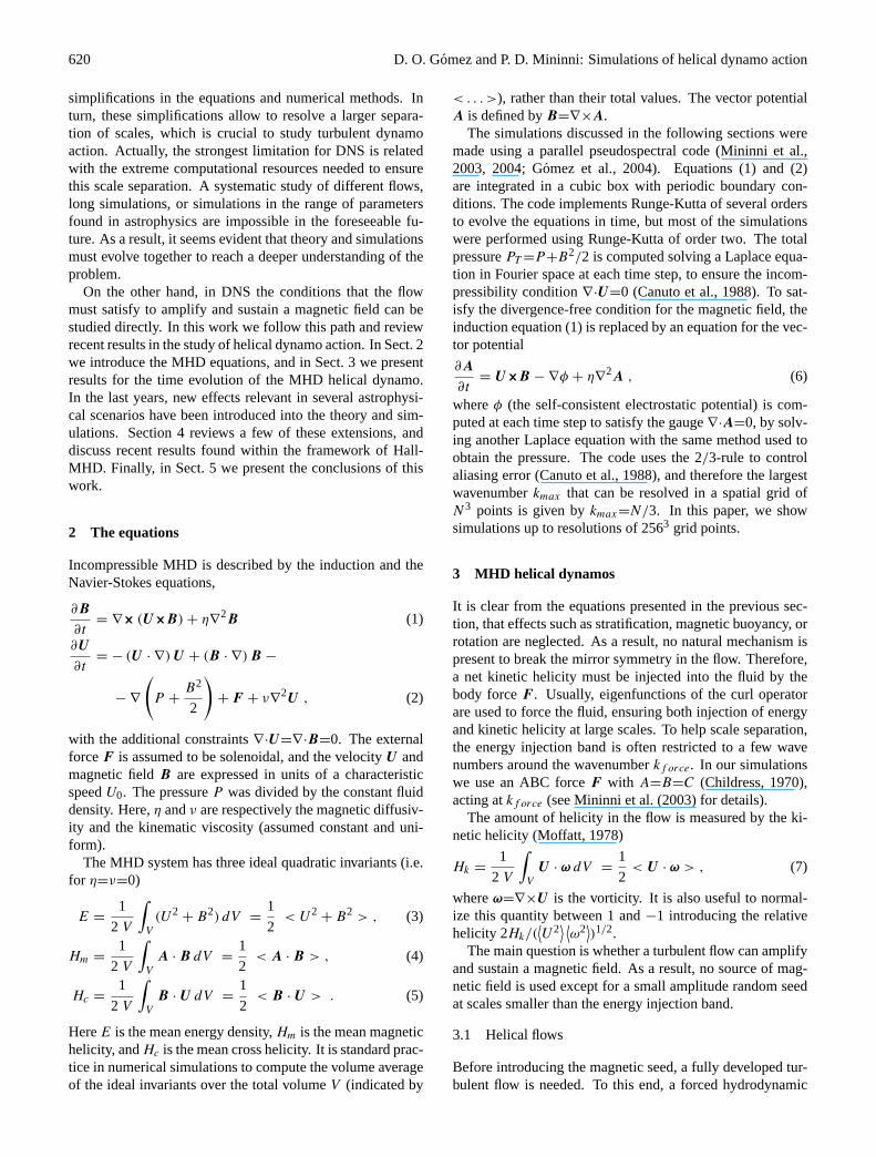
Fig. 7. Evolution of magnetic helicity (negative), in dynamo simu-lations with different Reynolds numbers ( }d~_�o�k���¾��� ).

Fig. 8. Spectrum of magnetic helicity at ¬©�¥� , normalized by themagnetic energy at each } . Note the peak and the change in signclose to }V~��i�k��� . Large scales are dominated by negative magnetichelicity, while the kinetic helicity of the flow is positive at all scales(see e.g. Figure 1.b).

power law [O��� | a , and during the kinematic regime all themagnetic modes grow with the same rate peaking at smallscales (Figures 5 and 6), saturation takes place first at thesmall scales. This was predicted by Pouquet, Frisch, andLeorat (1976) using the EDQNM closure. Indeed, equation(9) shows that the � -effect is quenched by the term ¸�P ·

,proportional to the current helicity at small scales.

During and after the saturation, the magnetic field isstronger than the velocity field at small scales (Figure 9).Note that the kinetic energy spectrum at small scales isquenched by the Lorentz force, and therefore velocity fluc-tuations at small scales are suppressed by the growing mag-netic field. The kinetic energy spectrum deviates from theKolmogorov’s law, and its slope is steeper than � c SJZ (seeFigure 9.b).

This effect can be seen more clearly as the Reynolds num-ber and the scale separation between the energy injectionband and the small scales are increased (Mininni, Gomez,

Fig. 9. Spectrum of kinetic (solid lines) and magnetic energy(dashed lines) during saturation at small scales, in a simulation with}V~��i�k���¢��� and �����T��� : (a) ¬�� � , (b) ¬���¿ , and (c) ¬���À .

and Mahajan, 2004). Figure 10 shows the compensated en-ergy spectrum

6 � [ � [#� | aTÁN� � | a in a simulation with [nf/gih Hkj �Z and � � cVe 1 , where Á is the energy injection rate. If theenergy spectrum

6 � [ � follows a Kolmogorov’s law in the in-ertial range

6 � [ � �m©Â Á � | a [ ��� | a , (12)

then the compensated spectrum should be flat in this range,and its amplitude corresponds to the Kolmogorov’s constantmÃÂ .

As can be seen from Figure 10, small scales are dominatedby the magnetic energy, and the kinetic energy spectrum issteeper than � c SVZ during the saturation. However, the totalenergy spectrum follows a Kolmogorov’s law. This powerlaw is satisfied by the total energy during the complete evo-lution of the dynamo (kinematic regime, saturation, and finalstate).

Fig. 7. Evolution of magnetic helicity (negative), in dynamo simu-lations with different Reynolds numbers (kf orce=3).

6 D. O. Gomez and P. D. Mininni: Simulations of helical dynamo action

Fig. 7. Evolution of magnetic helicity (negative), in dynamo simu-lations with different Reynolds numbers ( }d~_�o�k���¾��� ).

Fig. 8. Spectrum of magnetic helicity at ¬©�¥� , normalized by themagnetic energy at each } . Note the peak and the change in signclose to }V~��i�k��� . Large scales are dominated by negative magnetichelicity, while the kinetic helicity of the flow is positive at all scales(see e.g. Figure 1.b).

power law [O��� | a , and during the kinematic regime all themagnetic modes grow with the same rate peaking at smallscales (Figures 5 and 6), saturation takes place first at thesmall scales. This was predicted by Pouquet, Frisch, andLeorat (1976) using the EDQNM closure. Indeed, equation(9) shows that the � -effect is quenched by the term ¸�P ·

,proportional to the current helicity at small scales.

During and after the saturation, the magnetic field isstronger than the velocity field at small scales (Figure 9).Note that the kinetic energy spectrum at small scales isquenched by the Lorentz force, and therefore velocity fluc-tuations at small scales are suppressed by the growing mag-netic field. The kinetic energy spectrum deviates from theKolmogorov’s law, and its slope is steeper than � c SJZ (seeFigure 9.b).

This effect can be seen more clearly as the Reynolds num-ber and the scale separation between the energy injectionband and the small scales are increased (Mininni, Gomez,

Fig. 9. Spectrum of kinetic (solid lines) and magnetic energy(dashed lines) during saturation at small scales, in a simulation with}V~��i�k���¢��� and �����T��� : (a) ¬�� � , (b) ¬���¿ , and (c) ¬���À .

and Mahajan, 2004). Figure 10 shows the compensated en-ergy spectrum

6 � [ � [#� | aTÁN� � | a in a simulation with [nf/gih Hkj �Z and � � cVe 1 , where Á is the energy injection rate. If theenergy spectrum

6 � [ � follows a Kolmogorov’s law in the in-ertial range

6 � [ � �m©Â Á � | a [ ��� | a , (12)

then the compensated spectrum should be flat in this range,and its amplitude corresponds to the Kolmogorov’s constantmÃÂ .

As can be seen from Figure 10, small scales are dominatedby the magnetic energy, and the kinetic energy spectrum issteeper than � c SVZ during the saturation. However, the totalenergy spectrum follows a Kolmogorov’s law. This powerlaw is satisfied by the total energy during the complete evo-lution of the dynamo (kinematic regime, saturation, and finalstate).

Fig. 8. Spectrum of magnetic helicity att=5, normalized by themagnetic energy at eachk. Note the peak and the change in signclose tokf orce. Large scales are dominated by negative magnetichelicity, while the kinetic helicity of the flow is positive at all scales(see e.g. Fig.1b).

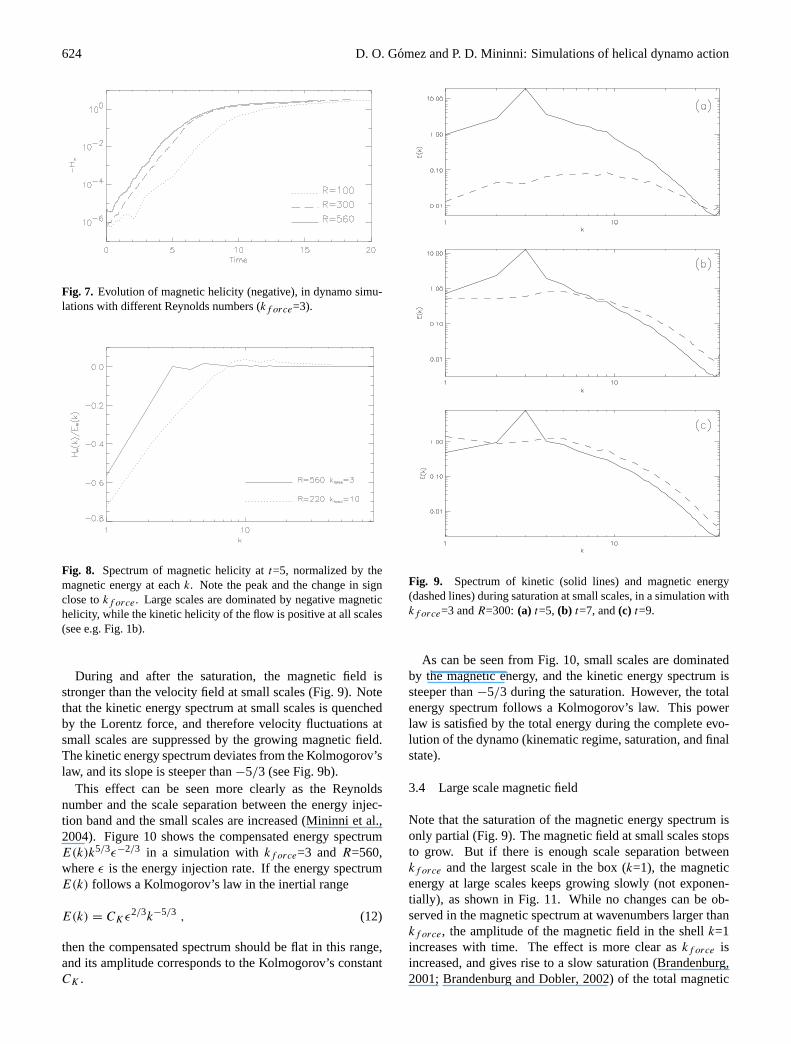
During and after the saturation, the magnetic field isstronger than the velocity field at small scales (Fig.9). Notethat the kinetic energy spectrum at small scales is quenchedby the Lorentz force, and therefore velocity fluctuations atsmall scales are suppressed by the growing magnetic field.The kinetic energy spectrum deviates from the Kolmogorov’slaw, and its slope is steeper than−5/3 (see Fig.9b).

This effect can be seen more clearly as the Reynoldsnumber and the scale separation between the energy injec-tion band and the small scales are increased (Mininni et al.,2004). Figure10 shows the compensated energy spectrumE(k)k5/3ε−2/3 in a simulation withkf orce=3 andR=560,whereε is the energy injection rate. If the energy spectrumE(k) follows a Kolmogorov’s law in the inertial range

E(k) = CKε2/3k−5/3 , (12)

then the compensated spectrum should be flat in this range,and its amplitude corresponds to the Kolmogorov’s constantCK .

6 D. O. Gomez and P. D. Mininni: Simulations of helical dynamo action

Fig. 7. Evolution of magnetic helicity (negative), in dynamo simu-lations with different Reynolds numbers ( }d~_�o�k���¾��� ).

Fig. 8. Spectrum of magnetic helicity at ¬©�¥� , normalized by themagnetic energy at each } . Note the peak and the change in signclose to }V~��i�k��� . Large scales are dominated by negative magnetichelicity, while the kinetic helicity of the flow is positive at all scales(see e.g. Figure 1.b).

power law [O��� | a , and during the kinematic regime all themagnetic modes grow with the same rate peaking at smallscales (Figures 5 and 6), saturation takes place first at thesmall scales. This was predicted by Pouquet, Frisch, andLeorat (1976) using the EDQNM closure. Indeed, equation(9) shows that the � -effect is quenched by the term ¸�P ·

,proportional to the current helicity at small scales.

During and after the saturation, the magnetic field isstronger than the velocity field at small scales (Figure 9).Note that the kinetic energy spectrum at small scales isquenched by the Lorentz force, and therefore velocity fluc-tuations at small scales are suppressed by the growing mag-netic field. The kinetic energy spectrum deviates from theKolmogorov’s law, and its slope is steeper than � c SJZ (seeFigure 9.b).

This effect can be seen more clearly as the Reynolds num-ber and the scale separation between the energy injectionband and the small scales are increased (Mininni, Gomez,

Fig. 9. Spectrum of kinetic (solid lines) and magnetic energy(dashed lines) during saturation at small scales, in a simulation with}V~��i�k���¢��� and �����T��� : (a) ¬�� � , (b) ¬���¿ , and (c) ¬���À .

and Mahajan, 2004). Figure 10 shows the compensated en-ergy spectrum

6 � [ � [#� | aTÁN� � | a in a simulation with [nf/gih Hkj �Z and � � cVe 1 , where Á is the energy injection rate. If theenergy spectrum

6 � [ � follows a Kolmogorov’s law in the in-ertial range

6 � [ � �m©Â Á � | a [ ��� | a , (12)

then the compensated spectrum should be flat in this range,and its amplitude corresponds to the Kolmogorov’s constantmÃÂ .

As can be seen from Figure 10, small scales are dominatedby the magnetic energy, and the kinetic energy spectrum issteeper than � c SVZ during the saturation. However, the totalenergy spectrum follows a Kolmogorov’s law. This powerlaw is satisfied by the total energy during the complete evo-lution of the dynamo (kinematic regime, saturation, and finalstate).

Fig. 9. Spectrum of kinetic (solid lines) and magnetic energy(dashed lines) during saturation at small scales, in a simulation withkf orce=3 andR=300: (a) t=5, (b) t=7, and(c) t=9.

As can be seen from Fig.10, small scales are dominatedby the magnetic energy, and the kinetic energy spectrum issteeper than−5/3 during the saturation. However, the totalenergy spectrum follows a Kolmogorov’s law. This powerlaw is satisfied by the total energy during the complete evo-lution of the dynamo (kinematic regime, saturation, and finalstate).

3.4 Large scale magnetic field

Note that the saturation of the magnetic energy spectrum isonly partial (Fig.9). The magnetic field at small scales stopsto grow. But if there is enough scale separation betweenkf orce and the largest scale in the box (k=1), the magneticenergy at large scales keeps growing slowly (not exponen-tially), as shown in Fig.11. While no changes can be ob-served in the magnetic spectrum at wavenumbers larger thankf orce, the amplitude of the magnetic field in the shellk=1increases with time. The effect is more clear askf orce isincreased, and gives rise to a slow saturation (Brandenburg,2001; Brandenburg and Dobler, 2002) of the total magnetic

D. O. Gomez and P. D. Mininni: Simulations of helical dynamo action 625D. O. Gomez and P. D. Mininni: Simulations of helical dynamo action 7

Fig. 10. Compensated spectrum of kinetic, magnetic and total en-ergy after saturation ( ¬©�5� ), in a simulation with }d~��o�����]�5� and��� �N�T� .

3.4 Large scale magnetic field

Note that the saturation of the magnetic energy spectrum isonly partial (Figure 9). The magnetic field at small scalesstops to grow. But if there is enough scale separation be-tween [ fTgih Hkj and the largest scale in the box ( [ � 7 ), themagnetic energy at large scales keeps growing slowly (notexponentially), as shown in Figure 11. While no changescan be observed in the magnetic spectrum at wavenumberslarger than [nf/goh Hkj , the amplitude of the magnetic field in theshell [ � 7 increases with time. The effect is more clear as[nf/goh Hkj is increased, and gives rise to a slow saturation (Bran-denburg, 2001; Brandenburg and Dobler, 2002) of the totalmagnetic energy (see Figure 4). The increase of magnetic en-ergy at large scales can also be observed in real space (Figure12).

The large scale magnetic field ( [ � 7 ) is an approximatelyforce-free field. Neglecting the mean flow � , assuming asolution of the form� � � 3�Ä/ÅÇÆÉÈ_Ê Ë4Ì�Í/Î , (13)

and replacing in the mean field equation (8), we finally obtainÏ � Æ 3 P � 3 � ¦�Ð ��� j f�fn[ � § � 3 L (14)

This equation is satisfied if� 3 is an eigenvector of the curl

operator, �WP � 3 �MÑ [d3 � 3 . Note that in this case theLorentz force � P �

at large scales is zero, and the hypoth-esis of negligible mean flow is consistent with the solution.Equation (14) only holds during the kinematic regime. How-ever figure 11.b shows that in the saturated state the spectrumat large scales is dominated by magnetic energy as [=f/gih Hkj isincreased, and Meneguzzi, Frisch, and Pouquet (1981) andBrandenburg (2001) verified in DNS of helical dynamo ac-tion that the magnetic field at [ � 7 is a force-free field.

Using this result, and the asymptotic conservation ofmagnetic helicity from equation (10), Brandenburg (2001)showed that the saturation of the amplitude of the large scalemagnetic field is achieved as$ � �o� � $ 3�Ò 7 � Ä � �{Ó p_ÔÈ�Õ Î � ΪÖ�×oØ�Ù�Ú L (15)

Fig. 11. Magnetic energy spectrum (thin lines) as a function oftime (from ¬q�X¿ up to ¬q�X�N� , time as in Figure 4), and kineticenergy spectrum at late times (thick line), during the last stage ofthe saturation of the dynamo: (a) }d~��o�k���Û�U� and �U�U�T��� , (b)}V~��i�k���Û�¹�_� and �U������� . Note the slow increase of magneticenergy at }9�+� .The time evolution of the amplitude of the large scale mag-netic field from DNS shows a good agreement with this re-lation (Brandenburg, 2001). Equation (15) indicates that thesaturation of the large scale field takes place in a resistivetime scale, and is dominated by the evolution of magnetichelicity.

Due to this build up of a coherent magnetic field witha correlation length of the size of the box, helical dy-namos (considered as dynamos produced by flows mostlydominated by one sign of kinetic helicity, as discussedat the beginning of this section) are often called “largescale dynamos”. This name is used in the literature inopposition to “small scale dynamos” where a non-helicalflow is studied (Kazantsev, 1968; Zeldovich, Ruzmaikin,

Fig. 10. Compensated spectrum of kinetic, magnetic and totalenergy after saturation (t=6), in a simulation withkf orce=3 andR=560.

energy (see Fig.4). The increase of magnetic energy at largescales can also be observed in real space (Fig.12).

The large scale magnetic field (k=1) is an approximatelyforce-free field. Neglecting the mean flowU , assuming asolution of the form

B = B0 eik0·x+σ t , (13)

and replacing in the mean field Eq. (8), we finally obtain

iαk0 × B0 =

(σ + ηeff k2

)B0 . (14)

This equation is satisfied ifB0 is an eigenvector of the curloperator,∇×B0=±k0B0. Note that in this case the Lorentzforce J×B at large scales is zero, and the hypothesis ofnegligible mean flow is consistent with the solution. Equa-tion (14) only holds during the kinematic regime. How-ever Fig.11b shows that in the saturated state the spectrumat large scales is dominated by magnetic energy askf orce

is increased, andMeneguzzi et al.(1981) andBrandenburg(2001) verified in DNS of helical dynamo action that themagnetic field atk=1 is a force-free field.

Using this result, and the asymptotic conservation of mag-netic helicity from Eq. (10), Brandenburg(2001) showed thatthe saturation of the amplitude of the large scale magneticfield is achieved as

B(t) = B0

[1 − e−2ηk2

0(t−tsat )]

. (15)

The time evolution of the amplitude of the large scale mag-netic field from DNS shows a good agreement with this re-lation (Brandenburg, 2001). Equation (15) indicates that thesaturation of the large scale field takes place in a resistivetime scale, and is dominated by the evolution of magnetichelicity.

Due to this build up of a coherent magnetic field with a cor-relation length of the size of the box, helical dynamos (con-sidered as dynamos produced by flows mostly dominated byone sign of kinetic helicity, as discussed at the beginning ofthis section) are often called “large scale dynamos”. Thisname is used in the literature in opposition to “small scaledynamos” where a non-helical flow is studied (Kazantsev,

D. O. Gomez and P. D. Mininni: Simulations of helical dynamo action 7

Fig. 10. Compensated spectrum of kinetic, magnetic and total en-ergy after saturation ( ¬©�5� ), in a simulation with }d~��o�����]�5� and��� �N�T� .

3.4 Large scale magnetic field

Note that the saturation of the magnetic energy spectrum isonly partial (Figure 9). The magnetic field at small scalesstops to grow. But if there is enough scale separation be-tween [ fTgih Hkj and the largest scale in the box ( [ � 7 ), themagnetic energy at large scales keeps growing slowly (notexponentially), as shown in Figure 11. While no changescan be observed in the magnetic spectrum at wavenumberslarger than [nf/goh Hkj , the amplitude of the magnetic field in theshell [ � 7 increases with time. The effect is more clear as[nf/goh Hkj is increased, and gives rise to a slow saturation (Bran-denburg, 2001; Brandenburg and Dobler, 2002) of the totalmagnetic energy (see Figure 4). The increase of magnetic en-ergy at large scales can also be observed in real space (Figure12).

The large scale magnetic field ( [ � 7 ) is an approximatelyforce-free field. Neglecting the mean flow � , assuming asolution of the form� � � 3�Ä/ÅÇÆÉÈ_Ê Ë4Ì�Í/Î , (13)

and replacing in the mean field equation (8), we finally obtainÏ � Æ 3 P � 3 � ¦�Ð ��� j f�fn[ � § � 3 L (14)

This equation is satisfied if� 3 is an eigenvector of the curl

operator, �WP � 3 �MÑ [d3 � 3 . Note that in this case theLorentz force � P �

at large scales is zero, and the hypoth-esis of negligible mean flow is consistent with the solution.Equation (14) only holds during the kinematic regime. How-ever figure 11.b shows that in the saturated state the spectrumat large scales is dominated by magnetic energy as [=f/gih Hkj isincreased, and Meneguzzi, Frisch, and Pouquet (1981) andBrandenburg (2001) verified in DNS of helical dynamo ac-tion that the magnetic field at [ � 7 is a force-free field.

Using this result, and the asymptotic conservation ofmagnetic helicity from equation (10), Brandenburg (2001)showed that the saturation of the amplitude of the large scalemagnetic field is achieved as$ � �o� � $ 3�Ò 7 � Ä � �{Ó p_ÔÈ�Õ Î � ΪÖ�×oØ�Ù�Ú L (15)

Fig. 11. Magnetic energy spectrum (thin lines) as a function oftime (from ¬q�X¿ up to ¬q�X�N� , time as in Figure 4), and kineticenergy spectrum at late times (thick line), during the last stage ofthe saturation of the dynamo: (a) }d~��o�k���Û�U� and �U�U�T��� , (b)}V~��i�k���Û�¹�_� and �U������� . Note the slow increase of magneticenergy at }9�+� .The time evolution of the amplitude of the large scale mag-netic field from DNS shows a good agreement with this re-lation (Brandenburg, 2001). Equation (15) indicates that thesaturation of the large scale field takes place in a resistivetime scale, and is dominated by the evolution of magnetichelicity.

Due to this build up of a coherent magnetic field witha correlation length of the size of the box, helical dy-namos (considered as dynamos produced by flows mostlydominated by one sign of kinetic helicity, as discussedat the beginning of this section) are often called “largescale dynamos”. This name is used in the literature inopposition to “small scale dynamos” where a non-helicalflow is studied (Kazantsev, 1968; Zeldovich, Ruzmaikin,

Fig. 11.Magnetic energy spectrum (thin lines) as a function of time(from t=7 up tot=20, time as in Fig.4), and kinetic energy spectrumat late times (thick line), during the last stage of the saturation of thedynamo:(a) kf orce=3 andR=300,(b) kf orce=10 andR=220. Notethe slow increase of magnetic energy atk=1.

1968; Zeldovichet al., 1983; Schekochihin et al., 2001, 2004;Haugen et al., 2003), and the magnetic field generated is cor-related on scales much smaller than the energy containingscales of the turbulence. However, we want to point out thata large scale magnetic field can in some cases be generatedwithout fully helical turbulence or a netα-effect. Anisotropicflows can generate large scale magnetic fields (Nore et al.,1997). As another example, in mean field theory there areterms in the mean electromotive force that can build a meanfield when theα coefficient is zero (Urpin, 2002). Theω×j

term in this expansion is also known to generate large scalemagnetic fields (Geppert and Rheinhardt, 2002).

626 D. O. Gomez and P. D. Mininni: Simulations of helical dynamo action8 D. O. Gomez and P. D. Mininni: Simulations of helical dynamo action

Fig. 12. Spatial density of magnetic energy in a MHD dynamo sim-ulation, at early times (above) and during the saturation (below).The increase in the amplitude of the field and in the correlationlength can be observed.

and Sokoloff, 1983; Schekochihin, Cowley, Maron, andMalyshkin, 2001; Schekochihin, Cowley, Taylor, Hammett,Maron, and McWilliams, 2004; Haugen, Brandenburg, andDobler, 2003), and the magnetic field generated is correlatedon scales much smaller than the energy containing scales ofthe turbulence. However, we want to point out that a largescale magnetic field can in some cases be generated with-out fully helical turbulence or a net � -effect. Anisotropicflows can generate large scale magnetic fields (Nore, Bra-chet, Politano, and Pouquet , 1997). As another example, inmean field theory there are terms in the mean electromotiveforce that can build a mean field when the � coefficient is

zero (Urpin, 2002). The stP�¸ term in this expansion is alsoknown to generate large scale magnetic fields (Geppert andRheinhardt, 2002).

4 Beyond the MHD approximation

One-fluid MHD, as presented in equations (1) and (2) andused in the previous section, is the standard framework usedfor describing dynamo action in astronomical objects. It isa good approximation for the solar dynamo and the geody-namo (Priest and Forbes, 2000). Also, one-fluid MHD oftenturns out to be a reasonable description of the large scale bulkdynamics of the fluid, as long as the fluid does not support asignificant electric field in its own frame of reference. In ide-alized DNS of dynamo action, MHD is often used to obtain alarger scale separation, since the introduction of two-fluid ef-fects would increase the computer resources needed to carryout the simulations.

The increase of computing power in the last years allowedthe study of some extensions to the MHD dynamo theory,relevant in some astrophysical scenarios characterized bylow temperatures, partial ionization, or collisionless plasmas.MHD cannot be expected to properly describe these plasmasbecause it fails to distinguish the relative motions betweendifferent species. A first step toward creating a more appro-priate theory for these objects might be to include the dom-inant two-fluid effects considering a generalized Ohm’s law.The most relevant effects for astrophysical applications areambipolar diffusion and the Hall effect (Zweibel, 1988; War-dle, 1999; Wardle and Ng, 1999; Balbus and Terquem, 2001;Sano and Stone, 2002). In this section, we will discuss recentextensions of dynamo theory to include these effects.

4.1 Ambipolar diffusion

Ambipolar diffusion is important in the evolution of mag-netic fields in protostars, proto-planetary circumstellar disks,as well as in the case of the galactic gas (Zweibel, 1988,2002; Sano and Stone, 2002; Brandenburg and Subramanian,2004). It is also relevant in the evolution of magnetic clouds(Zeldovich, Ruzmaikin, and Sokoloff, 1983). In the interstel-lar medium, ambipolar diffusion is believed to be the princi-pal mechanism responsible for breaking the frozen-in condi-tion for the magnetic field.

The ambipolar drift occurs because the magnetic field linesare attached to the plasma ions but not to the neutrals. TheLorentz force acting over the magnetized ions generates adrift between the ions and the neutrals. If collisions are fre-quent, the Lorentz force acting on the ions is balanced bycollisions with the neutrals. Under these assumptions, in apartially ionized medium with the bulk velocity � dominatedby the neutrals, the induction equation (1) takes the form�������¥��(ÜÝ�k� � Þ � P �¨� �àß���� ��� � , (16)

whereÞ �á�ªâ Ūã#Ååä � � z . Here, â Å is the ion mass density,

and ã#Ååä is the collision frequency between ions and neutrals.

Fig. 12.Spatial density of magnetic energy in a MHD dynamo sim-ulation, at early times (above) and during the saturation (below).The increase in the amplitude of the field and in the correlationlength can be observed.

4 Beyond the MHD approximation

One-fluid MHD, as presented in Eqs. (1 and 2) and usedin the previous section, is the standard framework used fordescribing dynamo action in astronomical objects. It is agood approximation for the solar dynamo and the geody-namo (Priest and Forbes, 2000). Also, one-fluid MHD oftenturns out to be a reasonable description of the large scale bulkdynamics of the fluid, as long as the fluid does not support asignificant electric field in its own frame of reference. In ide-alized DNS of dynamo action, MHD is often used to obtain alarger scale separation, since the introduction of two-fluid ef-fects would increase the computer resources needed to carryout the simulations.

The increase of computing power in the last years allowedthe study of some extensions to the MHD dynamo theory,relevant in some astrophysical scenarios characterized bylow temperatures, partial ionization, or collisionless plasmas.MHD cannot be expected to properly describe these plasmasbecause it fails to distinguish the relative motions betweendifferent species. A first step toward creating a more appro-priate theory for these objects might be to include the dom-inant two-fluid effects considering a generalized Ohm’s law.The most relevant effects for astrophysical applications areambipolar diffusion and the Hall effect (Zweibel, 1988; War-dle, 1999; Wardle and Ng, 1999; Balbus and Terquem, 2001;Sano and Stone, 2002). In this section, we will discuss recentextensions of dynamo theory to include these effects.

4.1 Ambipolar diffusion

Ambipolar diffusion is important in the evolution of mag-netic fields in protostars, proto-planetary circumstellar disks,as well as in the case of the galactic gas (Zweibel, 1988,2002; Sano and Stone, 2002; Brandenburg and Subramanian,2004). It is also relevant in the evolution of magnetic clouds(Zeldovichet al., 1983). In the interstellar medium, ambipo-lar diffusion is believed to be the principal mechanism re-sponsible for breaking the frozen-in condition for the mag-netic field.

The ambipolar drift occurs because the magnetic field linesare attached to the plasma ions but not to the neutrals. TheLorentz force acting over the magnetized ions generates adrift between the ions and the neutrals. If collisions are fre-quent, the Lorentz force acting on the ions is balanced bycollisions with the neutrals. Under these assumptions, in apartially ionized medium with the bulk velocityU dominatedby the neutrals, the induction equation (1) takes the form

∂B

∂t= ∇× [(U + λJ × B)×B] + η∇

2B , (16)

whereλ=(ρiυin)−1. Here,ρi is the ion mass density, andυin

is the collision frequency between ions and neutrals. Notethat in this approximationU i=U+λJ×B is the velocity ofthe ions, and Eq. (16) expresses that the magnetic field linesin the ideal case (i.e.η=0) are frozen to the ion velocity field.

Simulations with this modified version of the inductionequation have been made within the context of reconnec-tion in the interstellar medium (Zweibel and Brandenburg,1997), and the generation of sharp fronts together with achange in the reconnection rate of magnetic fields were ob-served. The effect of ambipolar diffusion in the dynamo wasstudied using a simplified model byZweibel (1988), and anα-effect was recovered from Eq. (16). It was shown thathelical turbulence can amplify a magnetic field under theseconditions, and ambipolar diffusion can alleviate the needof large turbulent diffusivity in some numerical models ofgalactic dynamos. More recentlyBrandenburg and Subra-manian(2000) confirmed the existence of anα-effect con-tributed by ambipolar diffusion, using both direct simulationsin a periodic box and a closure model.

D. O. Gomez and P. D. Mininni: Simulations of helical dynamo action 627

4.2 The Hall effect

The Hall effect is relevant in dense molecular clouds (Wardleand Ng, 1999), in accretion disks (including proto-planetarydisks) (Wardle, 1999; Balbus and Terquem, 2001; Sano andStone, 2002), in white dwarfs and neutron stars (Yakovlevand Urpin, 1980; Muslimov, 1994; Geppert and Rheinhardt,2002; Geppertet et al., 2003), and in the early universe(Tajima et al., 1992). Recently, the impact of the Hall cur-rent on the dynamo effect was also measured in the labora-tory (Ding et al., 2004).

With the inclusion of the Hall effect, the induction equa-tion (1) reads

∂B

∂t= ∇× [(U − εJ ) ×B] + η∇

2B , (17)

The Hall termεJ×B is the manifestation of the differencein velocity between ions and electrons. Indeed, in a two-species quasi-neutral electron-ion plasmaU e=U−εJ is theelectron velocity. From Eq. (17), whenη=0 the magneticfield is frozen to the velocity field, instead of the bulk veloc-ity U as is the case in one-fluid MHD.

Assuming the characteristic velocity equal to the Alfvenvelocity, the intensity of the Hall effect is given byε=c/(ωpiL0). Herec is the speed of light, andωpi is the ionplasma frequency. Note thatc/ωpi has dimensions of length(the ion skin depth), and corresponds to the lenghtscalewhere the Hall effect becomes non-negligible. General ex-pressions forε, as well as characteristic values for astrophys-ical objects can be found inMininni et al. (2003).

Since in Eq. (17) the magnetic field is stretched by theelectron velocity fieldU e rather than the bulk velocity fieldU , and these velocities can be quite different, the Hall termis expected to impact on dynamo mechanisms. The influenceof the Hall effect on the dynamo was studied in simplifiedmodels byHeintzmann(1983), and byGalanti et al.(1994).

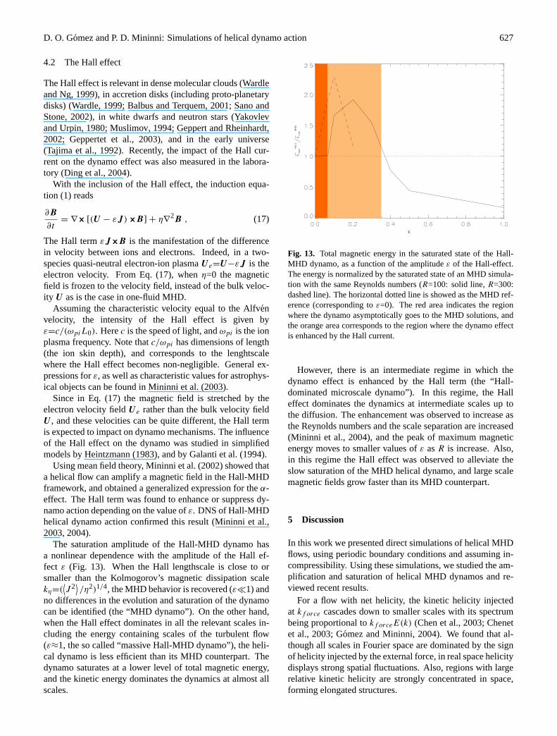
Using mean field theory,Mininni et al.(2002) showed thata helical flow can amplify a magnetic field in the Hall-MHDframework, and obtained a generalized expression for theα-effect. The Hall term was found to enhance or suppress dy-namo action depending on the value ofε. DNS of Hall-MHDhelical dynamo action confirmed this result (Mininni et al.,2003, 2004).

The saturation amplitude of the Hall-MHD dynamo hasa nonlinear dependence with the amplitude of the Hall ef-fect ε (Fig. 13). When the Hall lengthscale is close to orsmaller than the Kolmogorov’s magnetic dissipation scalekη=(

⟨J 2⟩/η2)1/4, the MHD behavior is recovered (ε�1) and

no differences in the evolution and saturation of the dynamocan be identified (the “MHD dynamo”). On the other hand,when the Hall effect dominates in all the relevant scales in-cluding the energy containing scales of the turbulent flow(ε≈1, the so called “massive Hall-MHD dynamo”), the heli-cal dynamo is less efficient than its MHD counterpart. Thedynamo saturates at a lower level of total magnetic energy,and the kinetic energy dominates the dynamics at almost allscales.

10 D. O. Gomez and P. D. Mininni: Simulations of helical dynamo action

Fig. 13. Total magnetic energy in the saturated state of the Hall-MHD dynamo, as a function of the amplitude ð of the Hall-effect.The energy is normalized by the saturated state of an MHD sim-ulation with the same Reynolds numbers ( �K���_��� : solid line,�(�����T� : dashed line). The horizontal dotted line is showed as theMHD reference (corresponding to ð���� ). The red area indicatesthe region where the dynamo asymptotically goes to the MHD so-lutions, and the orange area corresponds to the region where thedynamo effect is enhanced by the Hall current.

netic helicity seems to reach an asymptotic value. This be-havior was also found in the evolution of the magnetic energyby Archontis, Dorch, and Nordlund (2003).

Finally, we reviewed recent extensions made to the stan-dard MHD dynamo theory, to include kinetic effects relevantin several astrophysical scenarios, such as protostars, proto-planetary disks, the interstellar medium, white dwarfs, andneutron stars. The most important extensions to the theory inthese objects are ambipolar diffusion and the Hall effect.

The idealized conditions used in these dynamo simula-tions are far from astrophysical or geophysical applications.Also, the values of the Reynolds numbers considered hereare far away from realistic values for astrophysical or geo-physical flows. This is even more relevant when extensionsto one-fluid MHD are considered. The study of new ef-fects (as ambipolar drift or the Hall effect) introduces newlenghtscales, making the separation between physically rel-evant scales (e.g. the energy injection band, the Hall scale,and the dissipation scale) even harder. However, despite thefact that these studies are still performed under idealized con-ditions, the results are encouraging. The inclusion of neweffects in MHD dynamo mechanisms, can help the devel-opment of the theory under conditions more appropriate forastrophysical plasmas.

Acknowledgements. Use of computer time at the Bocha Beowulfcluster at the Departamento de Fısica (FCEN, UBA) is acknowl-edged. Research of DOG has been partially founded by grantX209/01 from the University of Buenos Aires and by grant PICT

03-9483 from ANPCyT. DOG is a member of the Carrera del In-vestigador Cientıfico of CONICET.

References

Archontis, V., Dorch, S. B. F., and Nordlund, A.: Dynamo action inturbulent flows, Astron. & Astrophys., 410, 759–766, 2003.

Armstrong, J. W., Rickett, B. J., and Spangler, S. R.: Electron den-sity power spectrum in the local interstellar medium, Astrophys.J., 443, 209–221, 1995.

Balbus, S. A., and Terquem, C.: Linear Analysis of the Hall effectin protostellar disks, Astrophys. J., 552, 235–247, 2001.

Balsara, D. and Pouquet, A.: The formation of large scale struc-tures in supersonic magnetohydrodynamic flows, Phys. Plasmas,6, 89–99, 1999.

Blandford, R.D., and Payne, D.G.: Hydromagnetic flows from ac-cretion discs and the production of radio jets, Monthly Not. R.Astr. Soc., 199, 883–903, 1982.

Borue, V., and Orzag, A.: Spectra in helical three-dimensional ho-mogeneous isotropic turbulence, Phys. Rev. E, 55, 7005–7009,1997.

Brandenburg, A.: The inverse cascade and nonlinear alpha-effect insimulations of isotropic helical hydromagnetic turbulence, As-trophys. J., 550, 824–840, 2001.

Brandenburg, A. and Dobler, W.: Large scale dynamos with helicityloss through boundaries, Astron. & Astrophys., 369, 329–338,2001.

Brandenburg, A. and Dobler, W.: Solar and stellar dynamos - latestdevelopments, Astron. Nachr., 323, 411–416, 2002.

Brandenburg, A. and Subramanian, K.: Astrophysical magneticfields and nonlinear dynamo theory, arXiv:astro-ph/0405052.

Brandenburg, A. and Subramanian, K.: Large scale dynamos withambipolar diffusion nonlinearity, Astron. & Astrophys., 361,L33–L36, 2000.

Braginsky, S. I.: Magnetogidrodinamika zemnovo yadra, Geomag-netizm i Aeronomiya, 4, 989–916, 1964.

Brandenburg, A., Saar, S.H., and Turpin, C.R.: Time evolution ofthe magnetic activity cycle period, Astrophys. J. Lett., 498, L51–L54, 1998.

Brissaud A., Frisch, U., Leorat, J., Lesieur, M., and Mazure, A.:Helicity cascades in fully developed isotropic turbulence, Phys.Fluids, 16, 1366–1367, 1973.

Buffett, B. A.: Earth’s core and the geodynamo, Science, 288,2007–2012, 2000.

Bullard, E.: The magnetic field within the Earth, Proc. Roy. Soc.London, A197, 433–453, 1949.

Canuto, C., Hussaini, M. Y., Quarteroni, A., and Zang, T. A.: Spec-tral Methods in Fluid Dynamics. Springer-Verlag, New York,1988.

Casse, F., and Keppens, R.: Radiatively inefficient magnetohydro-dynamic accretion-ejection structures, Astrophys. J., 601, 90–103, 2004.

Cattaneo, F. and Hughes, D. W.: Nonlinear saturation of the turbu-lent ñ effect, Phys. Rev. E, 54, R4532–R453, 1996.

Cattaneo, F.: On the origin of magnetic fields in the quiet photo-sphere, Astrophys. J. Lett., 515, 39–42, 1999.

Chen, Q., Chen, S., and Eyink, G. L.: The joint cascade of energyand helicity in three-dimensional turbulence, Phys. Fluids, 15,361–374, 2003.

Chen, Q., Chen, S., Eyink, G. L., and Holm, D.D.: Intermittencyin the joint cascade of energy and helicity, Phys. Rev. Lett., 90,

Fig. 13. Total magnetic energy in the saturated state of the Hall-MHD dynamo, as a function of the amplitudeε of the Hall-effect.The energy is normalized by the saturated state of an MHD simula-tion with the same Reynolds numbers (R=100: solid line,R=300:dashed line). The horizontal dotted line is showed as the MHD ref-erence (corresponding toε=0). The red area indicates the regionwhere the dynamo asymptotically goes to the MHD solutions, andthe orange area corresponds to the region where the dynamo effectis enhanced by the Hall current.

However, there is an intermediate regime in which thedynamo effect is enhanced by the Hall term (the “Hall-dominated microscale dynamo”). In this regime, the Halleffect dominates the dynamics at intermediate scales up tothe diffusion. The enhancement was observed to increase asthe Reynolds numbers and the scale separation are increased(Mininni et al., 2004), and the peak of maximum magneticenergy moves to smaller values ofε asR is increase. Also,in this regime the Hall effect was observed to alleviate theslow saturation of the MHD helical dynamo, and large scalemagnetic fields grow faster than its MHD counterpart.

5 Discussion

In this work we presented direct simulations of helical MHDflows, using periodic boundary conditions and assuming in-compressibility. Using these simulations, we studied the am-plification and saturation of helical MHD dynamos and re-viewed recent results.

For a flow with net helicity, the kinetic helicity injectedat kf orce cascades down to smaller scales with its spectrumbeing proportional tokf orceE(k) (Chen et al., 2003; Chenetet al., 2003; Gomez and Mininni, 2004). We found that al-though all scales in Fourier space are dominated by the signof helicity injected by the external force, in real space helicitydisplays strong spatial fluctuations. Also, regions with largerelative kinetic helicity are strongly concentrated in space,forming elongated structures.

628 D. O. Gomez and P. D. Mininni: Simulations of helical dynamo action

In simulations of helical dynamos, we reviewed the de-tailed evolution of magnetic energy and magnetic helicityduring the amplification and saturation stages. As we in-creased the Reynolds number, we found that the growth rateand the saturation level of the magnetic energy and the mag-netic helicity seems to reach an asymptotic value. This be-havior was also found in the evolution of the magnetic energyby Archontis et al.(2003).

Finally, we reviewed recent extensions made to the stan-dard MHD dynamo theory, to include kinetic effects relevantin several astrophysical scenarios, such as protostars, proto-planetary disks, the interstellar medium, white dwarfs, andneutron stars. The most important extensions to the theory inthese objects are ambipolar diffusion and the Hall effect.

The idealized conditions used in these dynamo simula-tions are far from astrophysical or geophysical applications.Also, the values of the Reynolds numbers considered hereare far away from realistic values for astrophysical or geo-physical flows. This is even more relevant when extensionsto one-fluid MHD are considered. The study of new ef-fects (as ambipolar drift or the Hall effect) introduces newlenghtscales, making the separation between physically rel-evant scales (e.g. the energy injection band, the Hall scale,and the dissipation scale) even harder. However, despite thefact that these studies are still performed under idealized con-ditions, the results are encouraging. The inclusion of neweffects in MHD dynamo mechanisms, can help the devel-opment of the theory under conditions more appropriate forastrophysical plasmas.

Acknowledgements.Use of computer time at the Bocha Beowulfcluster at the Departamento de Fısica (FCEN, UBA) is acknowl-edged. Research of DOG has been partially founded by grantX209/01 from the University of Buenos Aires and by grant PICT03-9483 from ANPCyT. DOG is a member of the Carrera delInvestigador Cientıfico of CONICET.

Edited by: P.-L. SulemReviewed by: two referees

References

Archontis, V., Dorch, S. B. F. and Nordlund,A.: Dynamo action inturbulent flows, Astron. & Astrophys., 410, 759–766, 2003.

Armstrong, J. W., Rickett, B. J. and Spangler, S. R.: Electron den-sity power spectrum in the local interstellar medium, Astrophys.J., 443, 209–221, 1995.

Balbus, S. A. and Terquem, C.: Linear Analysis of the Hall effectin protostellar disks, Astrophys. J., 552, 235–247, 2001.

Balsara, D. and Pouquet, A.: The formation of large scale struc-tures in supersonic magnetohydrodynamic flows, Phys. Plasmas,6, 89–99, 1999.

Blandford, R. D. and Payne, D.G.: Hydromagnetic flows from ac-cretion discs and the production of radio jets, Monthly Not. R.Astr. Soc., 199, 883–903, 1982.

Borue, V. and Orzag, A.: Spectra in helical three-dimensional ho-mogeneous isotropic turbulence, Phys. Rev. E, 55, 7005–7009,1997.

Brandenburg, A.: The inverse cascade and nonlinear alpha-effect insimulations of isotropic helical hydromagnetic turbulence, As-trophys. J., 550, 824–840, 2001.

Brandenburg, A. and Dobler, W.: Large scale dynamos with helicityloss through boundaries, Astron. & Astrophys., 369, 329–338,2001.

Brandenburg, A. and Dobler, W.: Solar and stellar dynamos – latestdevelopments, Astron. Nachr., 323, 411–416, 2002.

Brandenburg, A. and Subramanian, K.: Astrophysical magneticfields and nonlinear dynamo theory, arXiv:astro-ph/0405052,2004.

Brandenburg, A. and Subramanian, K.: Large scale dynamos withambipolar diffusion nonlinearity, Astron. & Astrophys., 361,L33–L36, 2000.

Braginsky, S. I.: Magnetogidrodinamika zemnovo yadra, Geomag-netizm i Aeronomiya, 4, 989–916, 1964.

Brandenburg, A., Saar, S. H. and Turpin, C. R.: Time evolution ofthe magnetic activity cycle period, Astrophys. J. Lett., 498, L51–L54, 1998.

Brissaud A., Frisch, U., Leorat, J., Lesieur, M., and Mazure, A.:Helicity cascades in fully developed isotropic turbulence, Phys.Fluids, 16, 1366–1367, 1973.

Buffett, B. A.: Earth’s core and the geodynamo, Science, 288,2007–2012, 2000.

Bullard, E.: The magnetic field within the Earth, Proc. Roy. Soc.London, A197, 433–453, 1949.

Canuto, C., Hussaini, M. Y., Quarteroni, A., and Zang, T. A.: Spec-tral Methods in Fluid Dynamics, Springer-Verlag, New York,1988.

Casse, F. and Keppens, R.: Radiatively inefficient magnetohydrody-namic accretion-ejection structures, Astrophys. J., 601, 90–103,2004.

Cattaneo, F. and Hughes, D. W.: Nonlinear saturation of the turbu-lentα effect, Phys. Rev. E, 54, R4532–R453, 1996.

Cattaneo, F.: On the origin of magnetic fields in the quiet photo-sphere, Astrophys. J. Lett., 515, 39–42, 1999.

Chen, Q., Chen, S., and Eyink, G. L.: The joint cascade of energyand helicity in three-dimensional turbulence, Phys. Fluids, 15,361–374, 2003a.

Chen, Q., Chen, S., Eyink, G. L., and Holm, D.D.: Intermittencyin the joint cascade of energy and helicity, Phys. Rev. Lett., 90,214503, 2003b.

Childress, S.: New solutions of the kinematic dynamo problem, J.Math. Phys., 11, 3063–3076, 1970.

Dikpati, M. and Charbonneau, P.: A Babcock-Leighton flux trans-port dynamo with solar-like differential rotation, Astrophys. J.,518, 508–520, 1999.

Ding, W. X., Brower, D. L., Craig, D., Deng, B. H., Fiksel, G.,Mirnov, V., Prager, S. C., Sarff, J. S., Svidzinski, V.: Measure-ment of the Hall dynamo effect during magnetic reconnection ina high-temperature plasma, Phys. Rev. Lett., 93, 045002, 2004.

Espagnet, O., Muller, R., Roudier, T., and Mein, N.: Turbulentpower spectra of solar granulation, Astron. & Astrophys., 271,589–600, 1993.

Galanti, B., Sulem, P.-L., and Gilbert, A. D.: Inverse cascades andtime-dependent dynamos in MHD flows, Physica D, 47, 416–426, 1991.

Galanti, B., Sulem, P.-L., and Pouquet, A.: Linear and non-lineardynamos associated with ABC flows, J. Geophys. Astrophys.Fluid Dyn., 66, 183–208, 1992.

Galanti, B., Kleeorin, N., and Rogachevskii, I.: Nonlinear dynamoin ABC flow: the Hall effect, Phys. Plasmas, 1, 3843–3849,

D. O. Gomez and P. D. Mininni: Simulations of helical dynamo action 629

1994.Geppert, U. and Rheinhardt, M.: Non-linear magnetic field decay

in neutron stars, Theory and observations, Astron. & Astrophys.,392, 1015–1024, 2002.

Geppert, U. Rheinhardt, M. and Gil, J.: Spot-like structures ofneutron star surface magnetic fields, Astron. & Astrophys., 412,L33–L36, 2003.

Gilbert, A. D.: Magnetic helicity in fast dynamos, Geophys. Astro-phys. Fluid Dynam., 96, 135–151, 2002.

Glatzmaier, G. A., Coe, R. S., Hongre, L., and Roberts, P. H.: Therole of the Earth’s mantle controlling the frequency of geomag-netic reversals, Nature, 401, 885–890, 1999.

Gomez, D. O., and Mininni, P. D.: Understanding turbulencethrough numerical simulations, Physica A, 342, 69–75, 2004.

Gomez, D. O., Mininni, P. D. and Dmitruk, P.: Parallel simulationsin turbulent MHD, Adv. Space Res., in press, 2004.

Haugen, N. E. L., Brandenburg, A. and Dobler, W.: Is nonhelicalhydromagnetic turbulence peaked at small scales?, Astrophys. J.Lett., 597, 141–144, 2003.

Haugen, N. E. L., Brandenburg, A. and Dobler, W.: Simulations ofnonhelical hydromagnetic turbulence, Phys. Rev. E, 70, 016308,2004.

Heintzmann, H.: The Hall effect in a unipolar inductor – A possi-ble mechanism for a dynamo and an antidynamo, J. Exp. Theor.Phys., 57, 251–259, 1983.

Hughes, D. W., Cattaneo, F., and Kim, E. J.: Kinetic helicity, mag-netic helicity and fast dynamo action, Phys. Lett. A, 223 167–172, 1996.

Kazantsev, A. P.: Enhancement of a magnetic field by a conductingfluid, Sov. Phys. JETP, 26, 1031–1034, 1968.

Kraichnan, R. H.: Helical turbulence and absolute equilibrium, J.Fluid Mech., 59, 745–752, 1973.

Krause, F. and Radler, K.-H.: Mean-Field Magnetohydrodynamicsand Dynamo Theory, Pergamon Press, New York, 1980.

Krishan, V., Paniveni, U., Singh, J., and Srikanth, R.: Relationshipbetween horizontal flow velocity and cell size for supergranula-tion using SOHO Dopplergrams, M. Not. R. Ast., 334, 230–232,2002.

Larmor, J.: How could a rotating body such as the sun become amagnet?, Brit. Assn. Adv. Sci. Rep., 1919, 159–160, 1919.

Leighton, R. B.: A magneto-kinematic model of the solar cycle,Astrophys. J., 156, 1–26, 1969.

Matsumoto, R., Uchida, Y., Hirose, S., et al.: Radio Jets and the For-mation of Active Galaxies: Accretion Avalanches on the Torusby the Effect of a Large-Scale Magnetic Field, Astrophys. J., 461,115–126, 1996.

Meneguzzi, M., Frisch, U., and Pouquet, A.: Helical and nonhelicalturbulent dynamos, Phys. Rev. Lett., 47, 1060–1064, 1981.

Meneguzzi, M. and Pouquet, A.: Turbulent dynamos driven by con-vection, J. Fluid. Mech., 205, 297–318, 1989.

Mininni, P. D., Gomez, D. O., and Mahajan, S. M.: Dynamo actionin Hall magnetohydrodynamics, Astrophys. J. Lett., 567, 81–83,2002.

Mininni, P. D., Gomez, D. O., and Mahajan, S. M.: Dynamo actionin magnetohydrodynamics and Hall-magnetohydrodynamics,Astrophys. J., 587, 472–481, 2003.

Mininni, P. D., Gomez, D. O., and Mahajan, S. M.: Direct Sim-ulations of Helical Hall-MHD Turbulence and Dynamo Action,Astrophys. J., in press, 2004.

Minter, A. H. and Spangler, S. R.: Observation of turbulent fluc-tuations in the interstellar plasma density and magnetic field onspatial scales of 0.01 to 100 parsecs, Astrophys. J., 458, 194–214,1996.

Moffatt, H. K.: Magnetic field generation in electrically conductingfluids, Cambridge University Press, Cambridge, 1978.

Muslimov, A. G.: Magnetic field evolution in neutron stars – cou-pling between poloidal and toroidal components in the crust, M.Not. R. Ast., 267, 523–528, 1994.

Nore, C., Brachet, M. E., Politano, H., and Pouquet, A.: Dynamoaction in the Taylor-Green vortex near threshold, Phys. PlasmasLett., 4, 1–3, 1997.

Parker, E. N.: Hydromagnetic dynamo models, Astrophys. J., 122,293–314, 1955.

Podvigina, O., and Pouquet, A.: On the non-linear stability of the1:1:1 ABC flow, Physica D, 75, 471–508, 1994.

Pouquet, A., Frisch, U., and Leorat, J.: Strong MHD helical turbu-lence and the nonlinear dynamo effect, J. Fluid Mech., 77, 321–354, 1976.

Priest, E. and Forbes, T.: Magnetic reconnection: MHD theory andapplications. Cambridge University Press, Cambridge, 2000.

Sano, T. and Stone, J. M.: The effect of the Hall term on the non-linear evolution of the magnetorotational instability, I. Local ax-isymmetric simulations, Astrophys. J., 570, 314–328, 2002.

Schekochihin, A., Cowley, S., Maron, J., and Malyshkin, L.: Struc-ture of small-scale magnetic fields in the kinematic dynamo the-ory, Phys. Rev. E, 65, 016305, 2001.

Schekochihin, A .A., Cowley, S. C., Taylor, S. F., Hammett, G. W.,Maron, J. L., and McWilliams J. C.: Saturated state of the non-linear small-scale dynamo, Phys. Rev. Lett., 92, 084504, 2004.

Seehafer, N.: Nature of theα effect in magnetohydrodynamics,Phys. Rev. E, 53, 1283–1286, 1996.

Steenbeck, M., Krause, F., and Radler, K.-H.: Berechnung der mit-tleren Lorentz-Feldstarke v×B fur ein elektrisch leitendendesMedium in turbulenter, durch Coriolis-Krafte beeinflußter Be-wegung, Z. Naturforsch., 21a, 369–376, 1966.

Tajima, T., Cable, S., Shibata, K., and Kulsrud, R. M.: On the originof cosmological magnetic fields, Astrophys. J., 390, 309–321,1992.

Tobias, S.: Relating stellar cycle periods to dynamo calculations,Monthly Not. R. Astr. Soc., 296, 653–661, 1998.

Urpin, V.: Mean electromotive force in turbulent shear flow, Phys.Rev. E, 64, 026301, 2002.

Wardle, M.: The Balbus-Hawley instability in weakly ionized discs,M. Not. R. Ast., 307, 849–856, 1999.

Wardle, M. and Ng, C.: The conductivity of dense molecular gas,M. Not. R. Ast., 303, 239–246, 1999.

Yakovlev, D. G. and Urpin, V. A.: On thermal and electrical conduc-tivities in neutron stars and white-dwarfs, Astr. Zh., 57, 526–536,1980.

Zeldovich, Ya .B., Ruzmaikin, A. A., and Sokoloff, D. D.: Magneticfields in astrophysics. Gordon and Breach, New York, 1983.

Zweibel, E. G.: Ambipolar diffusion drifts and dynamos in turbu-lent gases, Astrophys. J., 329, 384–391, 1988.

Zweibel, E. G. and Brandenburg, A.: Current sheet formation in theinterstellar medium, Astrophys. J., 478, 563–568, 1997.

Zweibel, E. G.: Ambipolar drift in a turbulent medium, Astrophys.J., 567, 962–970, 2002.