unit iii - bevel, worm and cross helical gears - SNS Courseware
Upload
khangminh22Category
view
1download
0
Cranfield University
MHMOD A A HAMEL
Condition Monitoring of Helical Gears Using Acoustic
Emission (AE) Technology
School of Engineering
Doctor of Philosophy
July, 2013


Cranfield University
School of Engineering
PhD Thesis
July, 2013
MHMOD A A HAMEL
Condition Monitoring of Helical Gears Using Acoustic
Emission (AE) Technology
Under Supervision: Prof. David Mba
Dr. A Addali
Academic Year 2012 - 2013
© Cranfield University, 2013. All rights reserved. No part of this publication may
be reproduced without the written permission of the copyright holder
i
ABSTRACT
Techniques such as vibration monitoring, thermal analysis and oil analysis are well
established as means to have been used to improve reliability of gearboxes and extend
time-to-failure. In this area Acoustic Emission (AE) technology is still in its infancy but
the attention shown by researchers towards this method has increased dramatically
because several studies have shown the AE offers the important advantage of improved
sensitivity over more conventional monitoring tools for the early detection and
prediction of gear failure.
Helical gear lubrication is critically important for maintaining the integrity of operating
gears and the oil also prevents asperity contact at the gear mesh thereby protecting the
gears from a deterioration process and surface failures. In gear systems, there are three
types of lubrication regimes: Dry Running, Boundary Lubrication (BL), Hydrodynamic
Lubrication (HL) and Elastohydro-dynamic Lubrication (EHL). The last regime is
associated with the normal operating running condition of gears.
Acoustic emissions were acquired from gears and analysed for different lubrication
regimes (dry, BL, HL and EHL regimes at different temperatures), and corresponding
specific film thicknesses (λ) levels. The results showed an inverse relationship between
AE signal levels and specific film thickness (λ) of the oil. This relation was used to
determine the lubrication regime from the measured AE signals. For instance, dry
running had the highest AE levels which were attributed to the metal-to-metal contact of
the gear mesh. The BL regime had relatively high AE levels which also attributed to the
level of asperity contact is greater than the oil film thickness. The HL regime was
characterized by the lowest AE levels due to the lubricant oil completely separating the
teeth during gear meshing. Finally, the EHL regime showed intermediate AE levels
compared to the BL and HL regimes because the oil film was less than for the HL
regime but greater than for the BL regime.
It is shown that the application of advanced signal processing methods is necessary for
monitoring helical gears; Kurtosis and Spectral Kurtosis were used to investigate the

ii
AE signatures and found to be effective in de-noising (spectral kurtosis) acquired
signals. Acoustic Emission proved to be a powerful tool to detect the oil regime for both
defective and non-defective conditions.
It is concluded that the experimental findings of this research programme will provide
the foundations for significant advancement in the application of AE for the
determining the lubrication regime present within a helical gearbox and for the detection
of developing gear faults. This should give a new impetus in the field of maintenance
and prevention of human and material catastrophes.
Several papers presenting the findings of this research have been published in
international journals and given at conferences.
Papers for Journals:
1. Journal of lubricants (mdpi): Using of Acoustic Emission for Monitoring Oil Film
Regimes. Manuscript ID (Research Paper): lubricants-34202 (published)
2. Journal of Engineering Tribology: Employing of Acoustic Emission for Monitoring
Oil Film Regimes. The number assigned to work (Research Paper) is TRIB-12-1205
(accepted)
3. Journal of Applied Acoustics: Investigation of the influence of oil film thickness on
helical gear defect detection using Acoustic Emission. the reference number:
APAC-D-13-00027 (accepted)
Papers for Conferences:
1. Oil Regime Monitoring in Helical Gears Using Acoustic Emission. M Hamel,
A Addali and D Mba. AMME-15 conference 29-31 May 2012 , Cairo, Egypt

iii
2. Employing acoustic emission for monitoring oil film regime. M Hamel,
A Addali and D Mba. The 51st Annual Conference of The British Institute of Non-
Destructive Testing, 11-13 September 2012, Northamptonshire, UK.ISBN: 978 0
903132 55 9
3. Investigation of the influence of oil film thickness on helical gear defect detection
using Acoustic Emission. M Hamel, A Addali and D Mba. CM 2013 and MFPT
2013, 18-20 June 2013, Kraków, Poland
4. Babak Eftekharnejad, Mhmod Hamel, Abdulmajid Addali and David Mba.
Condition Monitoring of Machinery in Non-Stationary Operations ,"Proceedings of
the Second International Conference "Condition Monitoring of Machinery in Non-
Stationnary Operations" CMMNO’2012", March 26 - 28, 2012 - Hammamet –
Tunisia, Part 4, 425-437, DOI: 10.1007/978-3-642-28768-8_45.

iv
Acknowledgment
First of all, I thank Allah, the almighty, for giving me the strength to carry on this
project. Next, I would like to express my gratitude to Department Power and Propulsion
of School of Engineering, Cranfield University, and specially to my supervisor Prof
David for the useful comments, remarks and engagement through the learning process
of this PhD thesis. Furthermore I would like to express my gratitude to staff of
Advanced Centre of Technology, ACT-Tripoli, and specially for Dr Mohmmed Ateeg
for introducing me to the topic as well for the support on the way. Also, I like to thank
everyone who helped me in my research, who have willingly shared their precious time
during the process of my research. I would like to thank my loved ones, who have
supported me throughout entire process. I will be grateful forever for you.
‘’ Deep gratitude and love for my parents, my wife, my children Aws and Farah and all
of my brothers and sisters’’

v
TABLE OF CONTENTS
ABSTRACT .................................................................................................. i
List of Tables ................................................................................................ 1
List of Figure s ............................................................................................. 2
1 Introduction .......................................................................................... 8
Project Aim and Objectives..................................................................... 11 1.1
Project Contribution ............................................................................... 11 1.2
2 Gears .................................................................................................... 14
Background ........................................................................................... 14 2.1
2.1.1 A historical Note ............................................................................. 14
2.1.2 Gear Types and Terminology ........................................................... 15
2.1.3 Helical Gears .................................................................................. 17
2.1.4 Advantages of Helical Gear .............................................................. 19
2.1.5 Gear Life Predictions ....................................................................... 20
Gear Lubrication .................................................................................... 21 2.2
2.2.1 Gear Tooth Temperature .................................................................. 22
2.2.2 Purposes of Lubrication ................................................................... 22
2.2.3 Lubricant Selection ......................................................................... 23
2.2.4 Lubrication Properties...................................................................... 23
Lubrication Methods .............................................................................. 24 2.3
2.3.1 Spray Lubrication (Forced oil circulation lubrication). ........................ 25
2.3.2 Splash Lubrication Systems .............................................................. 26
2.3.3 Grease Lubrication .......................................................................... 26
Lubrication Regimes in Gears ................................................................. 26 2.4
2.4.1 Boundary Lubrication (BL) .............................................................. 27
2.4.2 Elastohydrodynamic Lubrication (EHL) ............................................ 28
2.4.3 Hydrodynamic Lubrication (HL) ....................................................... 30
2.4.4 The Stribeck Curve .......................................................................... 31
Specific Oil Film Thickness (λ) ............................................................... 33 2.5
Gear Failures ......................................................................................... 37 2.6

vi
2.6.1 Lubrication Related Failures ............................................................. 39
2.6.2 Non Lubrication Related Failure ....................................................... 42
3 Gearbox Condition Monitoring Review: ......................................... 45
Signal Processing Techniques ................................................................. 46 3.1
Temperature Monitoring: ........................................................................ 52 3.2
Oil Debris Monitoring: ........................................................................... 53 3.3
Vibration analysis: ................................................................................. 57 3.4
Chapter 4 .................................................................................................... 60
Acoustic Emission ...................................................................................... 60
4 Acoustic Emission ............................................................................... 61
Brief history of Acoustic Emission .......................................................... 61 4.1
Acoustic Emission Sources ..................................................................... 62 4.2
Acoustic Emission Applications .............................................................. 64 4.3
Acoustic Emission’s, Advantages and Disadvantages ................................ 65 4.4
Acoustic Emission Sensors ..................................................................... 66 4.5
Sensor Couplant .................................................................................... 67 4.6
AE Measuring ....................................................................................... 69 4.7
Wear Conditions and Acoustic Emission .................................................. 71 4.8
Gear faults monitoring using acoustic emission. ........................................ 74 4.9
Acoustic Emission Activities Constraints ................................................. 75 4.10
Acoustic Emission and lubricant .............................................................. 75 4.11
Chapter 5 .................................................................................................... 78
Experimental Setup and procedure ......................................................... 78
5 Experimental Setup and procedure .................................................. 79
Experimental Gearbox ............................................................................ 79 5.1
5.1.1 Gears ............................................................................................. 81
5.1.2 Electrical Motor .............................................................................. 81
5.1.3 Lubrication ..................................................................................... 82
5.1.4 Loading Plates ................................................................................ 82
5.1.5 AE Sensors ..................................................................................... 83

vii
5.1.6 Thermocouples ............................................................................... 83
5.1.7 Slip Ring ........................................................................................ 84
5.1.8 Pre-Amplifier.................................................................................. 84
5.1.9 Accelerometers ............................................................................... 85
Data Acquisition (DAQ) Cards ................................................................ 85 5.2
5.2.1 Data Acquisition (DAQ) Software .................................................... 85
Experimental Procedure ......................................................................... 86 5.3
5.3.1 Capability of AE Technology for Gearbox Diagnosis .......................... 87
5.3.2 Influence of Lubrication Film Conditions on AE Signal ...................... 89
Chapter 6 .................................................................................................... 94
Results and Discussion .............................................................................. 94
6 Results and Discussion ....................................................................... 95
Capability of AE Technology for Gearbox Diagnosis ................................ 95 6.1
6.1.1 Test Instrumentation and Procedure .................................................. 95
6.1.2 Results Based on Acoustic Emission AE Monitoring .......................... 97
Influence of Lubrication Film Conditions on AE ..................................... 103 6.2
6.2.1 Test Instrumentation and Procedure ................................................ 103
6.2.2 Observations of AE Under Lubricated Conditions ............................ 104
Diagnosis During Dry and Lubricated Contact ........................................ 108 6.3
6.3.1 Test Instrumentation and Procedure ................................................ 108
6.3.2 Observations of AE Under Dry and Lubricated Conditions ................ 108
Applicability of AE in Monitoring Defects During Dry and Lubricated Contact6.4
112
6.4.1 Test Instrumentation and Procedure ................................................ 112
6.4.2 Observation of The Signals in Time and Frequency Domains ............ 113
Spectral Kurtosis of AE Signal from Defective and Non-Defective Gear ... 117 6.5
Correlation of AE r.m.s With Specific Film Thickness (λ) ...................... 126 6.6
General Observations ........................................................................... 127 6.7
Chapter 7 .................................................................................................. 128
Conclusions and Future Work ............................................................... 128
7 Conclusions and Future Work ........................................................ 129

viii
Conclusions ........................................................................................ 129 7.1
Future Work ........................................................................................ 131 7.2
8 References ......................................................................................... 134
9 Appendixes ........................................................................................ 148

1
List of Tables
Table 1: Ranges of tangential speed for gears (Handbook of metric gears, ). .................. 25
Table 2: Film thickness regimes, mechanisms and applications (Dowson, 1995; Dowson
and Ehret, 1999) ........................................................................................................ 27
Table 3: Specifications of helical gears used in the experimental work (Appendix A) ... 81
Table 4: Specification of the lubricant (Appendix C) ....................................................... 82
Table 5: K&J-type Thermocouple Specification (Appendix D for data sheet) ................ 83
Table 6: Experimental stages ............................................................................................ 93
Table 7: Estimated optimum frequencies and bandwidths from Kurtogram .................. 120

2
List of Figure s
Figure 1: Illustration of (a) spur and (b) helical gears (Gitin M, 1994) ....................... 14
Figure 2: Gear Types (Ham et al., 1958) ................................................................. 16
Figure 3: Gear Terminology (Ham et al., 1958) ....................................................... 16
Figure 4: Helical gear geometry (Becker and Shipley, 2002) ..................................... 18
Figure 5: Tooth contact lines on a spur gear (a), a bevel gear (b), and helical gear(c).
(Stokes, 1992) ............................................................................................... 19
Figure 6: Relative gear surface fatigue life as a function of (λ) (Townsend and Shimski,
1994) ............................................................................................................ 21
Figure 7: Lubricant spray arrangement (ASM., 1992) .............................................. 25
Figure 8: Splash (Bath) Lubrication System (Pirro and Wessol, 2001) ....................... 26
Figure 9: Boundary lubrication. (Richard Booser, P. D. (1983) ................................. 28
Figure 10: Distribution of pressure, temperature, pressure path in Hertz and film
thickness in an EHL contact (Dowson, 1977). ................................................... 29
Figure 11: Elastohydrodynamic Lubrication (EHL) (. Richard Booser, P. D. (1983) .... 30
Figure 12: Hydrodynamic lubrication (HL) (. Richard Booser, P. D. (1983) ............... 31
Figure 13: Stribeck Curve (Stribeck, 1902) ............................................................. 31
Figure 14 : Diagram of gear pair ............................................................................ 35
Figure 15: Gear failure modes ............................................................................... 38
Figure 16: Combination of sliding and rolling in gear teeth (Walton and Goodwin, 1998)
.................................................................................................................... 39
Figure 17: Stress distribution at and near contacting surfaces under rolling contact ..... 41
Figure 18: Modes of gear failures (Boyer, 1975) ...................................................... 43
Figure 19: condition based monitoring techniques ................................................... 46
Figure 20: Classical Bath-tub curve for wear (Roylance and Hunt, 1999) ................... 54
Figure 21: Schematic of the Acoustic Emission principle (NDT, 2013) ...................... 62
Figure 22: Example of Kaiser Effect (NDT, 2013) ................................................... 64
Figure 23: Schematic diagram of typical AE sensor(Miller and McIntire, 1987b) ........ 67
Figure 24: Hsu-Nielsen calibration head (Brüel and Kjaer., 1981) ............................. 68
Figure 25: Pencil lead break test raw signal, (Brüel and Kjaer., 1981) ....................... 69
Figure 26: Different AE signal types (Holroyd, 2000) ............................................. 70
Figure 27: The typical AE signal features (Physical Acoustic Co., 2007) ................... 71

3
Figure 28: Back-to-back gearbox ........................................................................... 79
Figure 29: Schematic diagram of the test arrangement .............................................. 80
Figure 30: Loading plates ...................................................................................... 83
Figure 31: Slip ring .............................................................................................. 84
Figure 32: Schematic diagram of the Data Acquisition Systems ................................ 86
Figure 33: Schematic diagram showing the different test positions at which the Nielsen
source was located ......................................................................................... 88
Figure 34: Seeded defect on single tooth ................................................................. 89
Figure 35: Cooling arrangement showing nitrogen gun nozzle .................................. 90
Figure 36: Liquid nitrogen gun location and gear wheel ........................................... 90
Figure 37: Defective gear ...................................................................................... 92
Figure 38: Schematic diagram of the experimental procedure ................................... 93
Figure 39: AE and vibration sensors locations ......................................................... 96
Figure 40: AE waveform associated with a defect free condition ............................... 98
Figure 41: AE waveform associated with a tooth defect ........................................... 98
Figure 42: Oil temperature with time; defect free and with seeded defect ................... 99
Figure 43: AE r.m.s values at each sensor with oil temperature ............................. 100
Figure 44: AE Energy values at each sensor with oil temperature ............................ 101
Figure 46: Statistical parameters of the AE first channel signals, a) kurtosis and b) Crest
Factor. ........................................................................................................ 102
Figure 47: Locations of the AE sensor and thermocouples ...................................... 103
Figure 48: Gear temperature, specific film thickness and AE r.m.s with lubrication
regime (system started dry, then oil was added and then system cooled). ........... 105
Figure 49: Influence of gear temperature and specific film thickness on AE waveforms
(the waveforms corresponded the regions in Figure 48) ................................... 107
Figure 50: Influence of gear temperature and specific film thickness on AE r.m.s
(system started dry, then oil was added and then system cooled). ...................... 109
Figure 51: Gear temperature, specific film thickness and AE r.m.s as Figure 50 but
enlarged ...................................................................................................... 110
Figure 52: Influence of gear temperature and specific film thickness on AE waveforms
(the waveforms correspond to the regions in Figure 50) .................................. 110
Figure 53: Defective Teeth – spalls of 2 mm diameter and 2 mm depth ..................... 112
Figure 54: Influence of gear temperature and specific film thickness on AE r.m.s ..... 113

4
Figure 55: AE waveforms associated with regions ‘A’, ‘B’, ‘C’ in Figure 54 ........... 114
Figure 56: Statistical parameters associated with AE waveform for different lubrication
regimes. ...................................................................................................... 116
Figure 57: Kurtogram for defect free test; waveforms ‘A’ to ‘D’ correspond to regions
‘A’ to ‘D’ in Figure 50 ................................................................................ 118
Figure 58: Kurtogram for defective gear test; waveforms ‘A’ to ‘D’ correspond to
regions ‘A’ to ‘D’ in Figure 54 ..................................................................... 119
Figure 59: AE waveforms associated with filtered signals (defect free test) ............. 121
Figure 60: AE waveforms associated with filtered signals (test with defective gear) .. 122
Figure 61: Effect of band pass filtering of raw AE signal on KURT and CF (Defect free
gear test) ..................................................................................................... 124
Figure 62: Effect of band pass filtering of raw AE signal on KURT and CF (defective
gear test) ..................................................................................................... 125

5
LIST OF EQUATIONS
……………………………………………………….….1 33
............................................................................2 33
..........................................................3 34
……......………………………………………. 4 34
……………………………………………...………5 34
.......................................................................6 35
........................................................ 7 35
......................................................................................................8 36
...............................................................................9 36
……………………………………...………..10 37
……………………………………………….....11 37
∫
……………………………………………………...12 47
r.m.s =√
∫
……………………………………………13 47
Fc = =
………………………..………………………………..….14 48
∑ ̅
………………………………………………...15 48
∫
……………………………………..16 51
……………………………………...…17 51

6
{| | }
| | …………………….……18 52
……………………………………..19 52

7
Chapter 1
Introduction

8
1 Introduction
Gearboxes are an essential component in all rotating machinery. A gearbox is a
transmission mechanism that provides both torque and speed conversions from a power
source that is rotating (such as an electric motor) to other devices in proportion to its gear
ratios. The often heavy financial losses associated with machine breakdown and
commercial pressure for greater efficiency, performance, and safety have made effective
machine fault detection and diagnosis increasingly important (Choy et al., 1994)
To ensure survival in the modern competitive market place it is vital for industries to
improve product reliability and simultaneously cut production costs. Product reliability is
particularly important for industries such as nuclear, aviation and petro-chemical where
failure can cause a serious environmental disaster. In particular the typical life of a wind
turbine is about 23 years (Luke, 2012), but there is considerable commercial pressure
increase this lifespan and improve productively, both of which will require effective
health monitoring of the gearbox.
Of particular note because they are so widely reported are helicopter accidents. Between
1964-1974, one fifth of UK helicopter accidents were caused by gearbox malfunction
(Tan, 2005; Le Sueur, 1978). The problem of faulty gearboxes in helicopters has not been
solved as witnessed by the report of the AAIB (UK Air Accidents Investigation Branch)
which blamed the North Sea helicopter crash of 1 April 2009 which killed 16 people on
gearbox failure (B. O. H, 2011). (McNiff, 1991) contains more reports on fatal aviation
accidents caused by gearbox failures. (Kar and Mohanty, 2006) have discussed
monitoring of helicopter transmission systems to avoid failure and the resulting
catastrophic accidents.
The correct choice of lubricant for a gearbox is essential for smooth running and long life
of gear boxes. The gear box is an important element of a wind turbine and it has been
reported that the right lubricant could save a typical operator as much as $5,000 year-on-
year per turbine operated (Luke, 2012). (Ashley, 2008) has reported that a survey of
experts working in different plants found that on average some 23 % of gear box failures
were attributed to either lack of lubricant or use of the wrong lubricant.

9
(Ribrant and Bertling, 2007) surveyed failures in Swedish wind power plants for the eight
years from 1997 to 2004. Their data shows that gearboxes can be a major source of wind
turbine breakdowns. Typically 20% of wind turbine downtime was due to gearbox
failure, with gearbox repairs taking an average of about 256 hours (Ribrant and Bertling,
2007)). A recent report by the Low Carbon Innovation Coordination Group (LCICG) has
emphasised the importance of energy from offshore wind turbines in the replacement of
elderly fossil fuel and nuclear plants. It is claimed that there could be a resultant saving of
as much as £89 billion of the UK’s energy bill, and that technological spin offs could take
a substantial share of a global market that could reach £1 trillion by 2050. Such a
development would have the added benefits of reducing the UK’s reliance on imported
gas and help meet GHG renewable energy and emission targets; The LCICG predicts that
UK companies could benefit from business opportunities worth up to £35bn from
offshore wind power. The report also predicts that given the necessary investment
offshore wind could deliver up to 50% of the UK’s total electricity generation by 2050
(ClickGreen, 2012)
The surveys in the public domain as reported by (Spinato et al., 2009) have revealed that
the gearbox has the longest downtime per failure for all onshore wind turbine sub-
assemblies, (Various, 2008; Faulstich, 2008) have revealed that gearbox faults account
for some 30% of all onshore lost wind turbine availability.
Early maintenance practices was breakdown strategy where an item was repaired only
when it broke down, this was also termed run-to-failure or unplanned maintenance. A
more advanced technique was preventive, or planned maintenance where the item was
removed from service, inspected and any necessary repairs or upgrading carried out at set
intervals, regardless of the health of the item. The relative complexity of modern products
and the production lines on which they are produced has increased the cost associated
with preventive maintenance until today it has become a major cost on production. Thus,
more efficient maintenance practices are being used, these include condition based
maintenance. For a good review of condition-based maintenance for detection and
diagnosis of faults see (Jardine et al., 2006).
Effective condition monitoring should detect the onset of a fault at an early stage and
provide a diagnosis of what the fault is and where it can be found. Ideally condition

10
monitoring should provide an all-round and detailed health assessment of the item of
equipment.
Condition based methods can be used for both production quality control and
maintenance planning, with the main benefits being cost savings and increased safety.
For maintenance, condition based monitoring is often used as an early warning system
which can be extremely useful in the process industries where unplanned shutdowns can
result in severe financial consequences or possibly even an accident involving working
personnel (Benbouzid, 2000). Condition based maintenance may necessitate significant
initial investment but can reduce overall costs by minimizing down-time and maximizing
the life time of items of equipment.
Today, condition monitoring usually means the application of advanced technology but
traditionally it has included visual and aural inspection (using the human senses), oil
analysis (also called wear debris analysis), temperature monitoring, airborne sound and
acoustic emission analysis, vibration measurement and analysis, and motor current
signature analysis. It has also included non-destructive testing.
Visual inspection although a basic form of condition monitoring can detect potential
failure modes such as leaking, cracking, corrosion, etc. Visual inspection should always
be carried out and other fo r.m.s of condition monitoring should augment it, (Keith,
2002)
Oil analysis is very useful for use with e.g. the gearboxes and bearings of wind turbines.
The measured levels of ferrous and non-ferrous particles in the lubricant give useful
information about the condition of the equipment. Trending is often used to predict faults
prior to failure (Tan et al., 2007).
Thermography is a well tried and tested method of condition monitoring and is especially
useful where heat is indicative of a fault as with electrical contacts, high speed bearings
or where there is metal-to-metal contact (Beattie and Rumsey, 1999) .
Using the vibration signal from a machine is a widespread as a method of condition
monitoring of rotating machinery as the vibration signal contains useful information
concerning the running condition of the machine (Tan et al., 2007; Lebold et al., 2000;
Mba and Rao, 2006).

11
Over the last few decades there has been a growing interest in using Acoustic Emission
for monitoring the condition of gearboxes. Recently Acoustic Emission has been shown
to be particularly useful in detecting and diagnosing fault formation at rolling contacts.
Acoustic Emission has a high frequency content, well above normal background, and so
is relatively insensitive to background noise, it is also highly sensitive to change in
machine condition but it has the disadvantage that the sensors must be place in close
proximity to the source(s) (Tan and Mba, 2005b; Tandon and Choudhury, 1999).
Project Aim and Objectives 1.1
The aim of this research is to use experimentally measured AE signals to identify and
classify lubrication regimes at gear mesh as a function of specific film thickness (λ). This
is to be achieved by measuring the AE signal as a function of lubricating oil and gear
metal temperature.
To achieve the objective it was necessary:
(i) To understand the effect of variations in the test operating temperatures on oil film
thickness and ability to identify the oil regime using AE technology.
(ii) To design and build a novel device to spray liquid nitrogen onto rotating gears, in-
situ, to reduce lubricant temperature whilst monitoring changes in AE.
(iii) To increase understanding of AE technology and its ability to monitoring helical
gears.
(iv) To investigate the condition on the AE signal produced due to a change in lubrication
regime of helical gears.
(v) Understand the influence on AE from studied natural surface fatigue under various
oil film regimes in real time operating gears.
(vi) To study the application of appropriate advanced signal processing techniques to
enhance the diagnostic effectiveness of AE signals to ascetain the lubricant regime.
(vii) To develop a relationship between oil film thickness and AE.
Project Contribution 1.2
The main contribution is the ability to effectively detect the oil film thickness
during helical gear mesh with the AE.

12
The outcomes of this research can contribute to a better and deeper understanding
of lubrication film classifications and their effects on gear performance and
service life efficiency.
It encourages the use of AE technology as an effective diagnosis technique in
lubrication-related failures of helical gear.
Results from this research program will establish a relationship between AE
technology and the lubrication regimes.

13
Chapter 2
Gears

14
2 Gears
Background 2.1
2.1.1 A historical Note
Gears are wheel-like elements within a machine which have teeth spaced uniformly
around their outer perimeters, see Figure 1. Gears have been in use for over 3000 years
(Gitin M, 1994) in rotating machines from clocks to giant transporters and vary in size
from a few mm to several metres in diameter
Gears are usually used in pairs, each on its own shaft, with the teeth of one meshing with
the teeth of the other which allows power to be transmitted from one shaft to the other
without slippage. When the gear teeth are meshed, turning one gear causes the other to
rotate. This set up allows the direction and speed of rotation of the driven shaft to be
changed. The gear with fewer teeth is the pinion. Speed of rotation is decreased when the
pinion drives the gear and increased when the gear drives the pinion. The speed reduction
factor is the ratio: = (number of gear teeth)/ (number of pinion teeth). Theoretically, when
the driven gear has three times the number of teeth of the driving gear it will rotate at
one-third the speed but deliver three times the torque.
Figure 1: Illustration of (a) spur and (b) helical gears (Gitin M, 1994)
a b
15
This control of speed and torque obtained by changing the relative number of teeth on the
gears is invaluable in industrial design and a large proportion of the world’s industry
depends on gears and gearing for its functioning (Manufacturing Association American
Gear, 1989).
2.1.2 Gear Types and Terminology
When considering their applications it is convenient to divide gears into one of three
groups. The differentiation is based on the different relative movements of the teeth when
meshing.
Figure 2 shows deferent types of gears. Spur gears have teeth which are cut parallel to
the shaft and are used to transmit power with parallel shafts. Spur gears produce no axial
thrust and this combined with their lower costs means spur gears are very widely used in
general machine applications of moderate speeds.
Helical gears - which are the subject of this study, are described in more detail in Section
2.1.3 - have their teeth cut at an angle, see Figure 1, which has the advantage that the
load is transferred progressively along the length of the tooth from one edge of the gear to
the other.
Bevel gears are used when quietness of operation is important. Bevel gears transmit
motion between shafts with intersecting centre lines (the intersecting angle is normally 90
deg). The teeth of bevel gears can also be cut in a curved manner to produce spiral bevel
gears, which produce smoother and quieter operation than straight cut bevels.
Other type of gears is worm and hypoid gears for high gear ratio, usually operate under
mixed friction conditions. Figure 3 shows some of the te r.m.s for gears (Ham et al.,
1958).

16
Figure 2: Gear Types (Ham et al., 1958)
Figure 3: Gear Terminology (Ham et al., 1958)

17
2.1.3 Helical Gears
An alternative to the spur gear are single helical gears where the teeth run around the
pitch cylinder in the form of a regular helix. Because of this helical shape the line of
contact the helical tooth makes with the mating gear is not parallel to the axis, as with
spur gears, but runs diagonally across the tooth face (Shigley et al., 2004). The helix
angle, an important parameter for helical gears is the acute angle which this line makes
with the axis, see Figure 4 and Appendix A and B. The helical gears may be viewed as
an infinite number of spur gears immediately adjacent to each other but with a relative
offset which in the limit combine to form a continuous smooth line, see Figure s 1 and 4
(Becker and Shipley, 2002). This slanted-line tooth contact is common to helical, hypoid
and spiral bevel gears. For equal standards of manufacturing accuracy helical gears have
a greater load carrying capacity and will transmit more power between parallel shafts
more quietly.
Helical Gear - Tooth Contact
The helical arrangement ensures tooth engagement is smooth and gradual and the load
more evenly distributed which gives quieter running and sudden shock loadings are
virtually eliminated. Figure 5 shows tooth contact lines for helical, straight spur and
bevel toothed gears. Of course, where single helical gears on parallel shafts are mated
they must both have equal helix angles, but in opposite directions, that is, they must be
opposite handed. To find the handing of a gear view the teeth on the end face looking
along the axis. If the teeth slope from bottom right to top left, the thread is a left handed
helix, if the teeth slope from bottom left to top right the thread is a right handed helix.
Careful selection of the helix angle ensures that the number of teeth in simultaneous
contact can be arranged to give the best compromise between mechanical efficiency and
smooth running. However, the helix angle means that a proportion of the force exerted by
the mating teeth is transmitted as an axial thrust along the shaft, and this must be allowed
for when choosing bearings to support the shaft.
The thrust on the bearings due to single helical gears can be overcome (to an extent) by
using double helical gears with opposing helix angles. These are more expensive and
require an increase in the width of the gears, but are widely used where quiet and smooth-

18
running gearing is important in the transmission of heavy loads at high speeds. They also
usually need longer and heavier shafting with larger capacity bearings (Stokes, 1992).
Figure 4: Helical gear geometry (Becker and Shipley, 2002)
Helical gears angel Ψ - between
the red and blue lines

19
Figure 5: Tooth contact lines on a spur gear (a), a bevel gear (b), and helical
gear(c). (Stokes, 1992)
2.1.4 Advantages of Helical Gear
In a helical gear train the teeth progressively engage rather than all at once. This
reduces noise generation and gives “silent” power transfer.
Is able to transfer power between non-parallel shafts, though with some loss of
efficiency.
The teeth of the helical gear are positioned diagonally (see Figure 1) and so are
effectively larger than the teeth on a spur gear. Hence, for same tooth size helical
gears can carry a greater load than a spur gear.
Suitable for high-speed, high-power transmission systems.
20
2.1.5 Gear Life Predictions
There are so many factors and indeterminacies that govern the life of gears (e.g.
alignment, load, lubrication, operating temperature, etc.) that predicting the remaining
useful life of a gear remains an inexact science. Nevertheless, based on experience it is
possible to usefully estimate the life of gears. A combination of accelerated life tests and
practical on-site experience is commonly used to predict the life of gears. This method
tends to be used conservatively to avoid catastrophic failure and so usually
underestimates the remaining life. The capability of predicting gear life more accurately
would allow the process of gear design to be undertaken with greater confidence, as well
as enabling greater length of working life.
Both the International Standards Organization and British Standards have developed
methods for estimating a gear’s strength and durability, allowing the life of the gear to be
estimated. Using BS 436-3:1986 as a basis, the British Gear Association (BGA) has
produced a software package (Gear Analysis Suite) which simplifies the load capacity
calculation for helical and spur gears and estimates the safety factor for these gears using
bending and contact stresses. It also takes into account a number of parameters such as
lubricant, gear material and tooth profile, etc. (Joseph, 2005).
The lubricant and its properties are clearly of vital importance in determining the life of
gears and it is now becoming increasingly clear that oil-film thickness is often over-
estimated by isothermal smooth surface analyses (Olver, 2002). Consequently it is
necessary to review the estimation of gear surface temperature to improve reliability of
film thickness calculations. Figure 6 shows that where the lubricant has a specific film
thickness greater than unity there is a rapid and substantial increase in surface fatigue life
(Townsend and Shimski, 1994).

21
Figure 6: Relative gear surface fatigue life as a function of (λ) (Townsend and
Shimski, 1994)
Gear Lubrication 2.2
An essential element of mechanical engineering is determining what takes place at the
interface when two machine components meet or touch. Whenever one surface slides
over another there is a frictional force. The common explanation for this is that the peaks
of the surface roughness (asperities) of the one surface interact with those of the other
surface, increasing the friction and possibly causing cause surface damage. Lubricants are
used to maintain separation of the surfaces and so reduce friction and wear. Lubricants
can also act to remove heat and protect against corrosion. To maintain the operation of
helical gears at the required power and speed appropriate lubrication and cooling are
necessary (Gitin M, 1994).
The duration of the working life of a gear is largely determined by the specific film
thickness (λ) of the lubricant. The specific film thickness is the ratio of the thickness of
the oil film to the composite surface roughness of the two gears in contact. It has been
shown that for elastohydrodynamic lubrication (EHL – see Section 2.4.2) λ is strongly
influenced by gear loading, speed and temperature (Dowson, 1977); Dowson and
Higginson, 1977).
λ

22
2.2.1 Gear Tooth Temperature
When gear trains are continuously operated important surface failure problems (e.g.
pitting, cracking and scoring) can occur due to thermal effects. High transient
temperatures can be generated by tooth contact and these heat up the surface of the gear,
sometimes at start-up when the layer of lubricant is thin the rate of temperature increase
is so great as to generate a thermal shock and thermo-cracking of the tooth surface and
break up (desorption) the layer of lubricant. Seireg (2001) has reported that transient
temperatures on the surface of the tooth and in the lubrication film have a significant
influence on surface pitting and wear.
Each cycle of heating and cooling generates microscopic changes in the structure of the
gear surface material which accumulate and eventually a network of microscopic cracks
appears on the gear surface. Thus, the monitoring and evaluation of the temperature of
the gear surface is important and a large number of reports and publications concerning
the prediction and evaluation of transient temperatures due to heat generation during
meshing are now available. For example, John et al., (1985) reviewed gear lubricant
selection and methods for tooth temperature prediction, and more recently Handschuh
and Kilmain (2002) reported on the thermal behavior of helical gear trains operated at
high-speed.
(J and Quin˜o´nez, 2004) concluded from their experimental research that the thermocou-
ple is a very practical and reliable means of surface temperature measurement for online
monitoring of gear conditions.
2.2.2 Purposes of Lubrication
Lubrication is primarily to reduce heat generation and wear between surfaces in contact
and with relative motion. Heat and wear can never be completely eliminated but they can
be reduced to acceptable or even negligible levels. Both heat generation and wear are due
to frictional forces and can be minimized by lowering the coefficient of friction between
the surfaces in contact.
(Pirro and Wessol, 2001) have described how lubrication is also used to prevent the
formation of rust by reducing oxidation and to seal the system against the ingress of dust

23
and water. With transformers it also provides insulation and with hydraulic fluid power
applications it can transmit mechanical power.
2.2.3 Lubricant Selection
Published standards are available to assist in the selection of lubricant for gear systems.
These take into account gear type, gear speed, operating sump temperature and lubricant
viscosity index to determine the lubricant that is the best for the given application (ASM.,
1992). The properties of the lubricant are listed in Section 2.2.4 and each needs to be
considered in the selection.
2.2.4 Lubrication Properties
The most important properties of lubricants for gears operating under typical or
conventional conditions are (Pirro and Wessol, 2001):
Viscosity. This is a measure of the lubricant’s resistance to flow. When the gear is
operational the viscosity is key in determining and maintaining the optimal
lubricant film thickness between moving surfaces (teeth). The viscosity will often
be different for different types of gearbox. Manufacturers will state the
appropriate viscosity limits which will be a compromise for the various operating
conditions for the unit.
Adherence is a measure of how well the lubricant sticks to the teeth of the gear. It
is very important because it ensures the maintenance of the lubricant layer
between the meshing teeth.
Resistance to Oxidation. The lubricant must resist oxidization. Large gear units
can contain several thousand litres of oil which is expensive to replace so the
lubricant must be remain serviceable as long as possible.
Resistance to Corrosion. Corrosion inhibitors are included in good quality gear
lubricants to prevent surface oxidation should the lubricant become contaminated
with water due to, for example, condensation.

24
High Film Strength and Oiliness. Modern lubricants often use additives to
increase the oil's natural film strength which maintains separation of the meshing
surfaces, Oiliness is important, especially in the case of worm gears, to reduce the
very high tooth friction.
Demulsibility is the property of rapid separation should the gear lubricant be
contaminated with water.
Extreme Pressure Properties are important to prevent possible welding and
consequent tearing of tooth surfaces when in contact under high pressure.
Prevent scuffing by using anti-scuff additives; Anti-scuff additives reduce
scuffing by forming thick films of high melting point metal salts on the surface
which prevent metal to metal contact which, when extensive, may cause scuffing.
Lubrication Methods 2.3
The lubrication conditions for spur and helical gear are basically same. The magnitudes
of the loads and sliding speeds are similar, and requirements for viscosity and anti-scuff
properties are virtually identical. As has been stated above, viscosity is one of the most
important lubricant properties, and the higher the viscosity, the greater the protection
against gear tooth failure. For critical applications, the specific film thickness, λ, should
be calculated using Dowson and Higginson equation (Dowson, 1995).
The method of applying the lubricant to the gear teeth depends primarily on the pitch line
velocity and there are three methods in general use:
1. Spray lubrication (forced oil circulation lubrication),
2. Splash lubrication (oil bath method), and
3. Grease lubrication.
The selection depends upon tangential speed (m/s) of gear teeth and shaft rotational
speed. Grease is a good lubricant to use at low speeds but splash and forced circulation
lubrication are more appropriate for medium and high speeds. Table 1 shows the three
basic lubrication methods with applicable speed ranges.

25
Table 1: Ranges of tangential speed for gears (Handbook of metric gears, ).
2.3.1 Spray Lubrication (Forced oil circulation lubrication).
The lubricant (oil) is supplied through jets placed on the incoming side of the gear mesh
for high pitch line velocities and for gears equipped with plain bearings. This method can
be used for even the fastest peripheral speeds met in gear systems (about 250 m/s). Oil is
sprayed through perforated or slotted nozzles onto the tooth flanks and contact zone
either at the initial or the final meshing zone, see Figure 7. It is assumed that it is more
beneficial for lubrication for oil to be sprayed onto the initial meshing zone, but cooling
is enhanced by oil sprayed onto the final meshing zone. ASM recommend the amount of
sprayed oil to be between 0.5 and 1.0 l/min per cm width of tooth depending on the heat
to be dissipated (ASM., 1992).
Figure 7: Lubricant spray arrangement (ASM., 1992)

26
2.3.2 Splash Lubrication Systems
Splash lubrication gear systems are considered the easiest to use but are limited to a low
pitch line velocities, up to about 5 m/sec for helical, spur and bevel gears, but less than
about 4 m/sec for worm gears. To avoid excessive churning with unwanted loss of power
the lubricant level should not be too high, see Figure 8. The bottom wheel, see Figure 8,
should dip into the lubricant to about twice the tooth length, possibly between 2 cm and 4
cm depending upon the diameter of the gear. (Pirro and Wessol, 2001) have suggested
that high speed, high power gear sets should use pressure circulating systems with oil
coolers to reduce churning.
Figure 8: Splash (Bath) Lubrication System (Pirro and Wessol, 2001)
2.3.3 Grease Lubrication
The third type is grease lubrication; is suitable for any low speed gear system.
Lubrication Regimes in Gears 2.4
Most gear failure mechanisms occur because the lubricant layer breaks down and the
surfaces of the teeth come into intimate contact. Lubrication minimizes or eliminates this
contact by ensuring the presence of a thin film between the components which supports
the necessary load. The lubrication must be such that the motion of the surfaces does not
remove the lubricant film. Any lubricant that is “used up”, i.e. removed from the system
must be replaced so the load between the components will remain supported. Table 2
lists the three lubrication regimes which are described by the specific film thickness ratio
(λ, lambda) and the mechanisms by which the film is formed (E. Richard Booser, 1983)

27
(Dwyer Joyce, 1995). (Copper, 1983; Kutz, 2006; Martin, 1978; Neale, 1995) all studied
specific film thickness (λ) and their findings regarding values of lambda were almost
compatible with those shown in Table 2.
Table 2: Film thickness regimes, mechanisms and applications (Dowson, 1995;
Dowson and Ehret, 1999)
Regime
Specific film
thickness or Lambda
ratio (λ)
Typical
Friction
Coefficient
Mechanism of
Film Formation
Typical
Applications
(b) Boundary
Lubrication
(BL)
λ<1 0.1-0.3
Surfaces not fully
separated. Thin chemical
layers reduce the tendency
of the asperities to adhere.
metal cutting,
bearing start-up or
shutdown
(d) Elasto-
hydrodynamic
Lubrication
(EHL)
1< λ<10 0.001-0.01
As hydrodynamic, but high
local pressure causes
increase in viscosity and
elastic deformation
rolling element
bearings, gears,
cams and tappets
(a) Hydrodynamic
Lubrication
(HL)
λ>10 0.01-0.03
Lubricant is dragged into
wedge between
components. The lubricant
pressure increase supports
the applied load
journal bearings,
machine slideways,
piston ring/liner.
2.4.1 Boundary Lubrication (BL)
Much research is being conducted to gain a better understanding of boundary lubrication,
where the lubricant acts as a protective barrier and the oil film thickness is greater than
the sum of surface roughness of both surfaces. However, most boundary lubricants are a
sacrificial film – in the sense that must be continually renewed - that only delays the
onset of friction and wear. A number of factors exist that can prevent a lubricant film
from forming. (Krantz and Kahraman, 2004) list these as: misalignment, interruption of
lubricant supply, lubricant with too low a viscosity, too high local temperatures, loads too
great for the lubricant to support, shock loads and low speeds.
Boundary lubrication exists when the lubricant film between sliding surfaces breaks
down and the gears meshing surfaces come into contact. This occurs at low speeds and
high loads, when the surfaces slide over each other, see Figure 9. The absence of an oil
film means the load is transferred to those areas of the sliding surfaces in direct contact,
which is only a small a fraction of the apparent area. At the microscopic level it is the

28
surface asperities which meet and create numerous micro scale grooves in the opposing
surface. In these circumstances the asperities are constantly being crushed and
restructured and in the process release bursts of energy in the form of Acoustic Emission
(AE) and local flash temperatures (Macconochie and Newman, 1961). The exact nature
of the surface interactions is not fully understood but in such a regime the properties of
the lubricant film are assumed to be unimportant.
Figure 9: Boundary lubrication. (Richard Booser, P. D. (1983)
2.4.2 Elastohydrodynamic Lubrication (EHL)
Figure 10 shows pressure and temperature distributions and film thickness for
Elastohydrodynamic Lubrication (EHL). Dowson (Dowson, 1995; Dowson and Ehret,
1999) has provided a wide-ranging history of the research into EHL during the 20th
century. Operating experience accumulated over many years of gearbox operation where
suitable lubrication was used, clearly pointed to metal-to-metal contact as a rare event
even in highly loaded gears. The conclusion was that a protective film of oil separated the
surfaces of the meshing gear teeth, thus EHL is considered the dominant mode of
lubrication for meshing surfaces such as bearings and gears.

29
Figure 10: Distribution of pressure, temperature, pressure path in Hertz and film
thickness in an EHL contact (Dowson, 1977).
(Dowson, 1977) has described how, initially, the minimum thickness of the lubricating oil
film between gear teeth was calculated on the basis of hydrodynamic theory alone but
this was found to be much less than the measured surface roughness of the gear teeth. By
the 1950s it was realised that the analysis had to include lubricant viscosity and local
elastic deformation. Dowson explains how this breakthrough resulted in a number of
empirical dimensionless expressions for minimum oil film thickness, in each of which the
minimum oil film thickness was strongly influenced by the properties of both the
lubricant and the gear teeth, and the speed of rotation. In practice the range of materials
involved is small so the lubricant film thickness is dominated by the speed of rotation so
much so that an increase in load has negligible effect, what happens is that the size of the
effective loading carrying region is increased.
Figure 11 shows typical features of EHL contact in te r.m.s of the surface contact
friction model. For continuity of mass flow of the oil film between the two meshing
surfaces, the product of film thickness and lubricant density must be constant. Over most
of the Hertzian contact zone (between the meshing surfaces, refer to Figure 7) the film
layer is assumed to be of constant thickness, though the fluid pressure can rise to large
values. As the oil flows out of the contact zone the fluid pressure quickly returns to that
in the body of the lubricant. This sudden drop in pressure creates a restriction or choke
point. In order to maintain the continuity of mass flow of the film, the mass flow at the

30
entraining end has to increase. Coupling this phenomenon and the geometrical form, a
secondary pressure peak arises at the exit end. This feature characterises EHL. The
magnitude of the secondary pressure peak always far exceeds the maximum Hertzian
pressure. It is also at this exit where the minimum film thickness is located. Minimum
film thickness usually is 80% of the central film thickness (Dowson, 1995; Johnson,
2012).
Figure 11: Elastohydrodynamic Lubrication (EHL) (. Richard Booser, P. D. (1983)
2.4.3 Hydrodynamic Lubrication (HL)
Hydrodynamic Lubrication (HL) is the regime where a continuous film of lubricant fully
supports the sliding surface hydrodynamically. In HL, a fluid layer of thickness, h, as
shown in Figure 12 is formed by the relative motion of the gear teeth, this film decreases
friction between sliding surfaces by separating the solid surfaces and replacing
mechanical friction with fluid friction, see Figure 9. Factors effecting HL formation
include oil film viscosity and temperature, and speed of the fluid flow. When applied
correctly, HL can substantially reduce friction with high speeds and loads, reduce
vibration, and substantially extend service life. Most industrial equipment such as
turbines, compressors, transmissions and bearings operates under this regime (William,
1992).

31
Figure 12: Hydrodynamic lubrication (HL) (. Richard Booser, P. D. (1983)
2.4.4 The Stribeck Curve
(Stribeck, 1902) performed a series of experiments on bearing friction and derived a
relationship between the applied load, the coefficient of friction (µ), dynamic viscosity of
the lubricating oil (η) and rotational speed (v), which is presented as the Stribeck curve in
Figure 13. The Stribeck curve confi r.m.s that the lubrication process can be divided into
the three regions (regimes): boundary lubrication h (film thickness) < R (surface
roughness), elastohydrodynamic lubrication h ≈ R and hydrodynamic lubrication h >> R.
Figure 13: Stribeck Curve (Stribeck, 1902)
Boundary
lubrication
Elastohydrodynamic and
mixed lubrication
Hydrodynamic lubrication
Fri
ctio
n C
oef
fici
ent
µ
ηv/w
< 𝑅
> 𝑅 ≈ 𝑅

32
With HL, the lubricant totally separates the two friction surfaces and lubricant viscosity is
the major factor determining the tribological characteristics. With EHL lubrication, three
factors dominate the tribological characteristics: the coefficient of elasticity between the
solid surfaces, the viscosity of the lubricant, and the relation between viscosity and
applied pressure. BL tribology is largely determined by frictional forces between the
surfaces in asperity contact and the action on those frictional forces of the lubricant
(including any additives) present between the friction surfaces. Because the determining
characteristic of BL is the actual contact made between the surfaces the hydrodynamic
properties of any lubricating oil are not a significant influence on the tribological
characteristics (Hamrock J et al., 2004).
(Macconochie and Newman, 1961) showed that the thickness of the lubricant film formed
between gear teeth is of the same order of magnitude as the surface roughness or the
diameter of foreign particles in the lubricant. Thus the film regime may be considered to
act hydrodynamically at the pitch line for all but the heaviest loads. If the gears are
heavily loaded, the lubrication will be quasi-hydrodynamic. The film regime conditions
depends upon the load, speed, tooth contour, surface finish, impurities in the lubricant
and lubricant viscosity. For a hydrodynamic film to be retained between two rolling
surfaces in contact strongly suggests additional mechanisms are at work – e.g. in high
speed rollers the transit time of the lubricant may be of the same order of magnitude as
the molecular relaxation time which determines the value of the viscosity and may cause
the lubricant to exhibit symptoms of shear rigidity. To calculate oil film thickness the
pressure viscosity may be used but pressure viscosity may not be used to calculate the
friction coefficient because the results obtained are far higher than found experimentally.
(Krantz and Kahraman, 2004) experimentally investigated the average wear rate of spur
gear pairs made from AISI 9310 steel, with lubricant viscosity and additives. Seven
lubricants with a range of viscosities were used to test gear tooth wear for gears that were
heat treated and case carburised. The measured wear was related to the elasto-
hydrodynamic film thickness, the contact fatigue lives of the specimens as determined in
the experiments, and the as-manufactured surface roughness. Typically, the rate of wear
was inversely proportional to the lubricant viscosity and specific film thickness (see
below). An exponential relationship was found between surface fatigue life and average

33
wear rates. The addition of different additives to lubricants with similar viscosities
produced different gear surface wear rates and fatigue lives.
Specific Oil Film Thickness (λ) 2.5
Specific film thickness (λ - lambda ratio) is strongly related to the lubricant viscosity,
temperature and surface roughness. Increasing λ can help to improve contact fatigue life
and a lambda ratio (λ) greater than 1 is usual for gears (Dowson, 1995);
……………….1
Where h is the thickness of the film of oil and σ r.m.s is a measure of the composite r.m.s
roughness of the two surfaces in frictional contact.
....................2
Where σ1 and σ2 are the r.m.s . surface roughnesses of the two surfaces in contact.
The problem can be simplified by assuming the two areas in frictional contact are
infinitely stiff, so that any wedging effect will depend only on the relative velocity of the
two surfaces and the lubricant. Such an assumption is valid only for low pressures. At
high pressures there will be deformation in the contact zone, and the increase in working
temperature will cause changes in the viscosity of the film. Both these need to be
included in any working model (Dwyer-Joyce, 1995). In fact, the viscosity of all
lubricants will generally increase as pressure increases and decrease as temperature
increases. These changes will be important for gears and rolling bearings which have
highly contact loads.
Viscosity will vary with temperature as given by the MacCoull equation (Alexander,
1992), and reference tables normally provide values of the lubricant viscosity at 40oC and
100oC (104
oF and 212
oF):
.......................3
Where

34
ν= Kinematic viscosity = η/ρ, (η = dynamic viscosity, ρ= density)
T= Absolute temperature, and
A and B = Constants for any given lubricant.
Re-arranging we obtain:
……......… 4
The manufacturer of lubricant provided values for the viscosity of Mobilegear type 636
used in these experiments at 40oC (680 cSt) and at 100
oC (39.2 cSt), see Appendix C. By
substituting these values into the equation for viscosity it was possible to solve for A and
B.
Mobilegear
Type 636
A=20.58
B=-3.26
Using results obtained by other workers and simplifying the physics of the situation by
assuming the load factor could be neglected and that for small temperature changes the
change in viscosity could also be neglected, Dowson and Higginson (Dowson, 1977)
obtained the following equation for oil film thickness:
……………………………5
Where: h= oil film thickness in µm,
ηo= dynamic viscosity in Pas,
u= entraining velocity in m/s, and

35
R= Equivalent radius in m.
Figure 14 : Diagram of gear pair
R can be obtained from:
...................6
u, entraining velocity, can be obtained from:
.......... 7
Where gear ratio,

36
......................................................8
r always expressed as a number larger than 1.
S= the distance between pitch line and contact point
R1 = pitch radius of the pinion
R2= pitch radius of the wheel
Ψ =Φ= pressure angle in Figure 14
N1 = rotational speed of pinion
To simplify the derivation, the contact between the meshing teeth will be assumed to be
on the pitch line, which implies S = 0, so Equations 6 and 7 simplify to:
..............9
u= V1 sin
Where
V1 is the pitch line velocity of pinion
Dynamic viscosity (cP) = Kinematics viscosity (cSt) * density(g/ml)
Or
Dynamic viscosity (Pas) = Kinematics viscosity (cSt) * (
)

37
………………..10
Where h is in µm
k = 1.6
E= modulus of elasticity (Pa)
w = load per unit length of cylinder (N/m)
α = pressure exponent of viscosity (Pa-1
)
Since:
and
F = Total load applied on the tooth/teeth (N),
d1 , d2 = Diameter of wheel and pinion (m),
T = Torque applied on the wheel shaft (Nm), and
l c = Line of contact length (m) (Appendix A and B).
The λ which used in this research was calculated as:
………....11
Gear Failures 2.6
Gearbox failures usually result from wear in the primary load carrying elements such as
gears, bearings and shafts. When gears fail there may be an increase in noise and
vibration levels but no further indication until total failure. However, each type of failure
imparts certain characteristics to the gear teeth, and (Peter Lynwander, 1983) has
38
described how a detailed examination can provide sufficient information to determine the
specific failure.
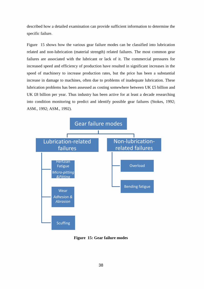
Figure 15 shows how the various gear failure modes can be classified into lubrication
related and non-lubrication (material strength) related failures. The most common gear
failures are associated with the lubricant or lack of it. The commercial pressures for
increased speed and efficiency of production have resulted in significant increases in the
speed of machinery to increase production rates, but the price has been a substantial
increase in damage to machines, often due to problems of inadequate lubrication. These
lubrication problems has been assessed as costing somewhere between UK £5 billion and
UK £8 billion per year. Thus industry has been active for at least a decade researching
into condition monitoring to predict and identify possible gear failures (Stokes, 1992;
ASM., 1992; ASM., 1992).
Figure 15: Gear failure modes
Gear failure modes
Lubrication-related failures
Hertzian Fatigue
Micro-pitting &Pitting
Wear
Adhesion & Abrasion
Scuffing
Non-lubrication-related failures
Overload
Bending fatigue

39
2.6.1 Lubrication Related Failures
Lubrication and cooling are necessary for the successful and efficient operation of helical
gear transmission systems. As helical gear teeth mesh the surfaces both roll and slide
against each other, see Figure 16, actions which can cause numerous failures.
Direct contact of tooth surfaces due to a lubrication related failure will generate stress at
and/or beneath the surface which can lead to tooth/gear failure. This has two fo r.m.s :
a- Micro-pitting along the pitch-line of gear teeth due to rolling contact fatigue.
b- Sliding-rolling contact fatigue which occurs in the gear teeth below the pitch-line
where negative sliding conditions exist. This can lead to surface pits which can then act
as the starting points for other failure modes.
Figure 16: Combination of sliding and rolling in gear teeth (Walton and Goodwin,
1998)
The lack or loss of lubricant between the gear teeth causes the teeth to rub against each
other and small particles of metal break loose. The areas in contact take on a roughened
appearance due to the consequent abrasive effects (sometimes called fretting corrosion)
Rolling contact
Sliding
Rolling

40
and red oxide debris may be seen. A badly worn surface is often produced very quickly if
the operation of a gear with the lubrication problem is not stopped. Unless remedial
action is taken the tooth will bend or break and the mesh disengages.
Lack of lubricant in gearboxes can usually be ascribed to damaged gaskets or seals, a
lubrication plug not re-inserted, oil leakage through inadequately sealed shaft keyways, or
an insufficient amount of lubrication used. There are no significant differences in the
lubrication problems which occur for spur gears as occur for helical gears.
Not only an adequate volume but the right lubricant must be used. That is, the lubricant
must have the correct viscosity to be thin enough to flow into the tooth mesh contact area
when cold but at operating temperatures and speeds is not too thin to support the tooth
mesh load. These conditions impose tight restrictions on the choice of lubricant and thus
an extreme pressure (EP) lubricant should be used (Fernandes and McDuling, 1997).
Pitting takes place due to metal fatigue and when the surface cannot withstand the high
Hertzian contact stresses. Small crack opens either on the tooth’s surface or just below
the surface. For sub-surface cracks, repeated cycling causes the crack to propagate nearly
parallel to the surface of the tooth for short distances before branching up to the tooth
surface, see Figure 17. Individual cracks can grow sufficiently long and in such a pattern
that small pieces of the surface layer are separated off and a pit is formed, see Figure 17.
Of course, adjacent cracks can have the same effect.
Spalling is when several small pits coalesce into a single large pit. Chemicals
(particularly hydrogen) contained in the water in lubricants can accelerate pitting of metal
surfaces, and metal particles carried with the lubricant can scratch the surface of the tooth
which enhances pitting by interrupting the continuity of the lubricant film as well as
causing stress concentrations, see Figure 18. Crack generation and pitting problems can
be reduced and even avoided by reducing the load to minimise contact stresses, ensuring
the surfaces of the gear teeth were carefully ground to be smooth, and properly heat-
treated.

41
Figure 17: Stress distribution at and near contacting surfaces under rolling contact
Micropitting: even when gears teeth have been surface hardened pitting can still take
place, though to a smaller depth, typically 10μm. Surfaces which have suffered
micropitting have a so-called frosted appearance, see Figure 18.
Adhesive: adhesive wear takes place when two surfaces rub together and material transfer
occurs. Mild adhesive wear does no more than disrupt the thin oxide layers on the
surfaces of the gear teeth. Severe adhesive wear is where the oxide layer is stripped away
and the bare metal of the gear tooth is exposed. Scuffing is severe adhesive wear, see
below.
Special care must be taken with gears operating at high loads and low speeds. Here
increasing the viscosity of the lubricant will significantly decrease adhesive wear, but
lubricants with chemically active extreme pressure additives should be avoided as they
are likely to be cause a high wear rate at low speeds and high loads.
Scuffing: occurs if the lubricant conditions are such that there are relatively large areas of
metal-to metal contact. The oxide films that protect the tooth surfaces are stripped away
and the bare metal revealed, which results in roughened surfaces and metal transfer from
one surface to the other. This can result in catastrophic damage if the teeth weld together
due to the frictional heat generated. New gear teeth are most vulnerable because their
surfaces have not been smoothed by running-in. The lubricants used in this situation
should contain anti-scuff additives which form a protective oxide layer at any local point
42
of high temperature by chemically reacting with the gear tooth’s surface. The oxide layer
once formed has a high melting point and remains as a solid on the surface of the tooth
even at high contact temperatures.
Scuffing is reduced by good alignment, rigid gear mounting and accurate machining of
the gear teeth. Scuffing will also be reduced if the temperature of the lubricant is
prevented from rising too high. This can be done by a heat exchanger in circulating-oil
systems. The materials used in the manufacture of the gears needs consideration, and
aluminium and stainless steel should be avoided. If there is any risk of scuffing, use
nitrided steel instead. Scoring of a gear tooth is similar effect to scuffing.
Abrasion: abrasive wear of gear teeth is invariably (and often) caused by particulate
contamination of the lubricant: spalled particles, sand or dirt particles taken in through
breathers, or particles that become added during maintenance. The spalled particles can
become work hardened when they pass between the gear teeth and are then especially
abrasive, so the use of oil filters in circulating-oil systems is essential. The use of filtered
breather vents and oil tight seals should minimize ingestion of contaminants. With
abrasive wear, inspection of gear teeth surfaces will reveal surface scratches.
Plastic flow: heavy loads combined with rolling and sliding action between gear teeth can
stress the material of the gear tooth beyond its elastic limit and deformation occurs
resulting in “fins” along the tops of the teeth.
2.6.2 Non Lubrication Related Failure
Non-lubrication-related failures tend to be tooth breakages which usually occur as result
of high levels of residual stress (e.g. due to an inclusion or cavity) in the region of the
root of the gear tooth, see Figure 18. Another cause of fracture or breakage of gear teeth
is the propagation of cracks due to overloading, impact or fatigue. With thin rims the
crack will start at the tooth root and travel through the gear resulting in catastrophic
failure (Joseph, 2005).

43
Figure 18: Modes of gear failures (Boyer, 1975)
Pitting
Spalling Crack
MicroPitting

44
Chapter 3
Gearbox Condition
Monitoring Review
45
3 Gearbox Condition Monitoring Review:
When monitoring the condition of gearboxes it is important to have the ability to detect
faults early, but the reliability of such detection must be high or there could be
unwarranted and costly shut downs of plant and production lines. Faults which progress
at a slow rate, if detected early, do not require immediate action. On the other hand, it is
essential not to confuse e.g. bending fatigue which can rapidly lead to catastrophic
failure, with pitting on gear teeth, which progresses at a slow rate and may even heal
over. In some industries such as the aircraft industry prevention of catastrophic failure is
put at a premium.
(Forrester, 1996) suggested catastrophic failure and can be prevented by;
1. Early detection at the beginning of the failure mode and rapid replacement of the
component well before catastrophic failure occurs, and
2. Reduction of the probability of failure, either by redesign of the component and/or
monitoring the component’s usage and replacing it when the probability of failure
exceeds a set threshold limit.
To detect and correctly diagnosis an imminent failure, suitable methods for collecting and
quantitatively analysing and assessing the necessary data, and a good understanding of
the failure mode are all necessary. Many faults are easily detectable if the component in
question can be removed and subjected to a series of tests: microscopy, X-ray, etc. Such
methods have an important place during manufacture, assembly and overhaul, but they
are often impractical in an operational system such as a plant production line or
helicopter transmission. In such circumstances non-intrusive methods need to be used for
routine condition monitoring.
Where the signal to be monitored is generated by the gear(s) any failure mode of the
rotating elements will cause changes in the vibration signature. They may also increase
the local temperature or produce material debris in the lubricant. Unlike industrial plant
and machinery where vibration monitoring is widely used and is often the system of
choice, few helicopters used temperature and oil debris monitoring (Forrester, 1996).
Figure 19 illustrate a diagram for types of condition monitoring techniques.

46
Figure 19: condition based monitoring techniques
Signal Processing Techniques 3.1
Gearbox fault detection was traditionally carried out by monitoring the vibration signal
and extracting certain statistical parameters. The extracted features were correlated with
particular faults within the gearbox. The most common of these parameters was the r.m.s
value of the time domain signal which was taken as a direct measure of the vibration
energy. (Samuel and Pines, 2005) have described other statistical parameters of interest
for condition monitoring, these included Kurtosis and Crest Factor. These parameters and
the associated theory are presented by (Samuel and Pines, 2005). The basis of the
technique was (Samuel and Pines, 2005) work reviewed a report by Stewart describing
how changes in the gearbox vibration signal were produced by damage to the gear(s) and
McFadden's mathematical model for generation of gearbox vibration signals (McFadden,
1986).
Until the mid-1970s the statistical indices were invariably extracted from the time domain
signal (Drouillard, 1988; Miller and McIntire, 1987b). However, with increased memory
and more rapid processing it has been possible to transform the time domain signal into
the frequency domain using, for example, the Fast Fourier Transform (FFT). With the
CBM
Oil Analysis
Vibration Analysis
Motor Current Signature Analysis
Thermography NDT Ispection
visual inspection
Ultrasonic Monitoring

47
time domain signal the energy at all frequencies is summed by the r.m.s value thus, to be
detected, a fault must have developed to an extent that the “fault energy” is of sufficient
magnitude to be detectable over the general background. In the frequency domain, on the
other hand, the energy of each frequency component can be seen. By trending the growth
in vibrational energy at a particular frequency a fault can be detected well before would
be detected in the time domain signal (Jardine et al., 2005). The vibration spectrum of a
gearbox contains a range of characteristic frequencies and their side bands, e,g, the tooth
mesh frequency, its harmonics and sidebands. It has been found both experimentally and
from theoretical analysis that when gearbox faults occur they have their own
characteristic frequencies. When these frequencies are detected in the spectrum they can
be used to classify gearbox faults (Henning, 1988).
Both time and frequency domain signals can be characterised using the same statistical
parameters, e.g. r.m.s , Crest Factor and Kurtosis. Creast Factor CF is the measure of the
relative energy above and below the mean signal level. Those parametres of interest to
this project are described in more detail below.
The techniques for analysing Acoustic Emission (AE) signals may be considered simply
as an extension of those used with vibration signals. The essential difference is that the
frequency range for AE is much higher than for vibration.
Time domain analysis: The most common statistical parameters extracted from the
time domain vibration signal for fault detection are the peak value, r.m.s (measure of
signal energy), Crest Factor, Kurtosis and the duration of specific events.
The mean value,
∫
……..12
Root mean square ( r.m.s ): is a measure of the power content of the signal and is defined
as follows (Broch, 1973):
r.m.s =√
∫
……………..13

48
Where x(t) is the instantaneous value of the time signal being analysed and T is the period
of measurement.
Crest factor: is a measure of the number and sharpness of the peaks in the signal. The
higher the crest factor the more “peaky” the signal. A high value for the vibration signal
from a bearing would normally be taken as an indication of the presence of a fault
(Yesilyurt, 1997; AlKazzaz et al., 2003).
Crest Factor, Fc = Peak value / r.m.s =
…….14
Where P is the peak value of the signal: P = max(x) – min(x)
Kurtosis for a signal which is digitally sampled is given by:
∑ ̅
……15
Where xi is the value of the ith
sample, N is the total number of samples,
x is the mean of
the samples and σ is the standard deviation of the samples. The “-3” is a normalisation
factor included so that the Gaussian/Normal distribution has K=0. A “peaky” signal will
have K > 0 and, conversely, a high value of K usually means the signal includes a number
of extreme peaks.
Kurtosis has been successfully used to detect and discriminate between different faults
but it has a significant weakness. If the fault is allowed to grow, the signal gradually loses
its “peakiness” and the K value decreases and ceases to be useful in detecting the fault
(Naid et al., 2009)
Consider two signals S1 = x1(t) and S2 = x2(t). Suppose S1 contains the greater energy; then
the r.m.s S1 > r.m.s S2. It is also possible for S1 and S2 to simultaneously have the same

49
peak values but the time-domain of S2 to be spikier than that of S1. In this situation we the
K value (and crest factor) for S2 would be larger than for S1.
Frequency domain analysis: The Fourier transform produces a frequency spectrum
which is the average of the input signal over the sampling period. It does not show how a
signal spectrum changes with time (Ruqiang, 2007) Today, the Discrete Fast Fourier
Transform (DFFT) is the most popular method of deriving it (Mathew, 1989). Decades of
practical application have confirmed frequency-domain analysis can reliably identify
frequency components within the signal indicative of a faulty condition of one or more
components. In practice the frequency components identifying the presence of a fault
may show themselves not as peaks in their own right but as sidebands to particular
frequencies in the spectrum and it is the change in the amplitude of these sidebands that
indicates the presence of mechanical problems in, say, a gear. Indeed, condition
monitoring of gearboxes invariably uses frequency domain analysis precisely because the
failure modes associated with each component have their own characteristic frequencies
(Muller and Errichello, 2001).
Where the signal is stationary the FFT is very useful, but many signals contain transient
phenomena including step changes, and these cannot be adequately analysed by FFT. The
Short-Time Fourier Transform (STFT) which analyzes only a small section of the signal
at a time was developed to overcome this problem. The STFT is able to map the signal
into both time and frequency providing useful information about both. The precision is
limited and determined by the window’s width (Da Silva, 1997) and (Liu et al., 1997).
Time-frequency domain analysis: Despite their usefulness there are occasions
when time domain and frequency domain analyses cannot characterise a fault. In such
circumstances to extract useful condition information from the vibration signal time-
frequency domain analysis is widely used.
Time-frequency domain (wavelet) analysis: is a procedure which contains variable-sized
windowing; using longer duration windows when accurate frequency information is
required, and shorter duration windows when accurate time information is needed.
Wavelets do not use the term “frequency” nor do we refer to time-frequency domains,

50
rather we speak about time-scale depiction where scale is an inverse function of
frequency. Wavelet analysis has attracted significant attention as a diagnostic tool for
condition monitoring and is recommended as an effective tool for detecting faults in gears
and bearing faults which are difficult to detect by the other frequency analysis methods
(Tse et al., 2004; Gaberson, 2002).
The Fourier transfo r.m.s the time-domain signal in te r.m.s of trigonometric functions
(sine and cosine); the wavelet transform expresses a signal in te r.m.s of known standard
“mother” wavelet functions which makes it more useful for the extraction of transient
features contained in a signal. Because these wavelets are of variable scale - the scale can
be varied by contraction/expansion and translation of the mother wavelet (window
function) - wavelet analysis can scrutinise the entire spectrum when extracting a fault
signal.
Wavelet analysis has the major advantage that it can characterise a signal localised in
time (non-stationary signals). This property is valuable for extracting information on
small magnitude changes in the signal and separates the wavelet transform from other
signal analysis methods.
Spectral Kurtosis: spectral kurtosis was introduced by (Dwyer, 1983) as a technique able
to distinguish between stationary signals and impulses and other transients in a
background of Gaussian noise. Spectral kurtosis has a high value for a frequency band
where the signal is dominated by impulses, and a low value for a frequency band where
the signal is dominated by stationary periodic components or Gaussian noise.
Recently, however, spectral kurtosis has also been applied for this purpose. Spectral
kurtosis was first introduced some twenty years ago but recently has it been applied to
fault detection in rotating machines (Antoni, 2004).
Spectral kurtosis was originally used to detect randomly occurring signals. Equally it can
be used to detect non-Gaussian components in a signal, e.g. structural vibrations in a
machine generated by a gear fault such as a cracked tooth. (Antoni, 2006) provides the
theoretical background to spectral kurtosis together with many references and examples
of its application to machine diagnostics including determining the frequency of the
excited component. (Antoni and Randall, 2006) and (Sawahli and Randall, 2004) present

51
the application of spectral kurtosis to the detection and diagnosis of faults in gears and
bearings.
(Sawahli and Randall 2004) concluded “spectral kurtosis is an exciting new analysis
technique for use in the diagnostics of rolling element bearing faults”. They claim it can
identify the frequency band that will provide most information on the presence of a fault
without the necessity of comparison of the “faulty” spectrum with the baseline healthy
spectrum. In this way the spectral kurtosis can aid fault detection and diagnosis by
providing information on what filters to use to isolate the most impulsive sections of a
signal spectrum from stationary masking (stationary components).
With spectral kurtosis it is useful to consider the vibration signal (say) to be stationary
Gaussian white noise modulated by a time and frequency varying complex envelope
function H(t,f) (Antoni, 2006). If signal Y(t) is defined as the system response at
frequency f, then
∫
…….16
With real machine vibration H(t,f) should be presented as H(t,f,w) because it is a
stochastic process. Here w is introduced as a random variable which represents time
variations. When H is time stationary and independent of the process X, we obtain a
conditionally non-stationary process (CNS).
Spectral kurtosis is a fourth-order spectral cumulant of a conditionally non-stationary
process:
…………………17
Where S2
nY(t,f) is second-order instantaneous moment and a measure of the energy of the
complex envelope:

52
{| | }
| | ………18
Thus, the spectral kurtosis is defined as the energy normalized cumulant (Antoni, 2004)
which is a measure of the peakiness of the probability density function H:
………………..19
The kurtogram was suggested by (Antoni and Randall, 2006) as a means of designing a
band-pass filter which can be applied to increase the signal–to-noise ratio. The kurtogram
is a 2-D map of the values of the spectral kurtosis calculated for various baqndwidths and
frequencies. Originally the kurtogram was based on the STFT but now it uses a filter
bank approach which gives the same quality of result but requires less calculation time –
this is the fast kurtogram which will be used here (Antoni, 2007).
The method will thus include following main steps (Antoni, 2007):
1. “Calculate the fast kurtogram of the vibration signal”.
2. “Design the bandpass filter based on the results of the kurtogram”.
3. “Analyse the filtered signal”.
Since a cracked tooth should generate impulses at a characteristic gear frequency,
analysis will focus on identifying the presence of such a signal.
Temperature Monitoring: 3.2
(Townsend and Akin, 1981) have shown that tooth load and tooth modification are the
most important factors in determining the temperature attained by the gearbox oil, and
toothed gears meshing under EHL produce a considerably higher temperature in the
lubricant than for direct contact of the tooth surfaces. Secondary factors include oil
viscosity and gear rotational speed. Further investigation of such factors as tooth shape

53
should help in determining optimum temperatures of lubricants under EHL conditions
(Wiśniewski and Janczak, 1981).
Present methods of temperature monitoring are not sufficiently sophisticated to determine
the temperatures of specific components and are used to indicate overheating due to such
problems as insufficient cooling and/or loss of lubricant. The effects of rotational speed,
load and meshing point on the gear tooth surface temperature have been investigated for a
spur gear using miniature type-K thermocouples. Maximum surface temperature was
found to occur on the dedendum. It was also shown that thermocouples are a practical
and reliable means of on-line CM of gears (J and Quin˜o´nez, 2004).
Temperature measurements of the tooth flanks has been achieved using thermocouples
which were glued as closely as possible to the areas of interest. The electronic evaluation
unit that was used provided a digital output to a PC for subsequent analyses. (Peter. J and
Stefan, 2001) claim that this his method produced accurate measurement of the
temperature for gearbox surface and lubricating oil temperatures. These results were then
used to estimate viscosity of the lubricant, wear, etc.
During continuous operation the gearbox temperature will arise until it reaches a stable
temperature, when heat generated within the gearbox equals the heat lost. The heat
generation is due to friction between the gears, hydrodynamic friction between the
lubricant and the moving components (during gear meshing, in the bearings and at the
seals) and overcoming viscous forces in the lubricant. These heat sources are, typically
are less than the heat generated when a fault or malfunction is present and this is offers a
method of monitoring the condition of gearboxes. Temperature can be measured by a
variety of thermal sensors such as thermometers, thermocouples, thermographic paints,
and thermal cameras (Pekka, 2006); (Cairns, 1991).
Oil Debris Monitoring: 3.3
Oil debris analysis is a widely used condition monitoring technique, from the technician
who rubs the oil debris between finger and thumb to spectrometric oil analysis and

54
scanning electron microscopy. The fault must have progressed sufficiently for enough
debris to be carried by the oil to the collection site for the fault to be detected. Careful and
detailed monitoring can indicate the type of component (e.g., gear teeth), type of failure
(e.g., spalling) and rate of degeneration. Unfortunately, while oil debris monitoring
cannot differentiate between two components of the same material, spectrometric oil
analysis has proved to be second only to acoustic emission techniques in detecting pitting
rates (Tan et al., 2007).
Trending is a common practice with wear debris analysis. Figure 20 shows the classic
Bath-tub curve for wear over the life of a gear. During running-in wear is high which
produces a lot of debris. Once the system has “settled in” and is properly lubricated the
rate of wear reduces to a low level. With time the gear shows signs of fatigue and the
rate of wear increases rapidly (Neale, 1995)(Evans and Hunt, 2008; Hamzah and Mba,
2009).
Figure 20: Classical Bath-tub curve for wear (Roylance and Hunt, 1999)
Wear occurs if two surfaces rub against one another with sufficient normal force.
However, adequate lubrication between the surfaces prevents the occurrence of wear
when the lubricant is clean, there is no overloading, temperature remains within
acceptable limits, etc. Excessive loading will cause the gear teeth to come into contact
and the material removed from contacting surfaces (wear debris) will contaminate the

55
lubricant and can be detected by lubricant monitoring. The analysis of the lubricant to
determine its condition can be off-line or continuously working (on-line). Both methods
usually use representative samples of the oil, though sometimes with the on-line method
all the oil flow passes through the measuring devices. Wear particles can be sorted and
collected by means of magnetic chip detectors (MCD). Most measurements concentrate
of detecting and analysing the solid debris to determine wear and need for oil additives.
Many techniques are used for wear metal analysis, for example spectrometric oil analysis
(SOA). Before analysis of oil samples using spectroscopic methods pre-treatment is
usually required. In SOA, an inductively coupled plasma (ICP) technique is used with an
Atomic Emission spectrometer. The oil sample is subjected to a high-voltage plasma
which energises the atomic structure of metallic elements present and the emitted light
can then be analysed. The wavelengths and intensity of this light determine the elements
present in the debris and their concentration.
However, oil analysis methods cannot identify faults such as fatigue cracks because such
as these failures may not generate metal particles (Tan et al., 2007; Pekka, 2006).
Debris analysis is, of course, intimately linked to EHL film thickness for lubricants. Thus
debris wear detection and analysis has also been used successfully for the detection
adequate lubricant thickness able to provide a protective film and control surface distress
in lubricated highly stressed components such as gears.
Some researchers have detailed the influence of load, speed and material properties on
the Elastohydrodynamic pressure distribution between solids and the thickness of the oil
film separating them (Bankim and Bernard, 1882). Speed and material of gears tend to be
the most important factors influencing the behaviour of the secondary pressure peak;
which is the result of the local pressure peak far in excess of the Hertzain maximum
which effectively reduces the film thickness at that position by approximately a further
25%(Dowson, 1977). However, as the range of materials is very small in practice, the
speed factor is the dominant variable.
In evaluating the EHL, (Tan et al., 2007) assumed the contacting surfaces were flat.
However in practice, particularly in gears, the contacting surfaces may be rough, leading
to asperity contact between the meshing surfaces even with the presence of a lubricant

56
film. The ratio of the minimum lubricant thickness to surface roughness will determine
the rapidity with which surface fatigue failures such as pitting and wear occur.
(Czichos, 1977) was performed experimental work with two different types of
equipment; line contact conditions were realised with a disc-on-flat tribometer, point
contact conditions were obtained using a ball-flat contact or ball-ball contact tribometer.
Experimental evidence indicates that the changeover from partial EHD to full asperity
contact is accompanied by only a small increase in the friction coefficient and may
therefore be overlooked if friction is not continuously recorded (with high resolution)
during the whole failure test. With full asperity contact, the onset of incipient scuffing is
determined by the stability of the asperity surface films, which in turn are affected by the
metal-lubricant interactions and the existence of the initial surface oxide films. It was
concluded that a criterion predicting the failure of sliding concentrated contacts should
take into account the physical and chemical nature of protecting surface layers as well as
the EHD and asperity contact conditions.
The FZG gear test rig system was used to study and observe the affect of oil temperature
on gear failures such as wear, pitting, micropitting and scuffing. High temperatures lead
to low viscosities, thin lubricant films and high chemical activity with good tribological
layer formation in the gear mesh which generally has a detrimental influence on failure
performance. At higher temperatures and thus lower viscosities and film formation
decreases, adhesive forces decrease and chemical activity is increased (Höhn and
Michaelis, 2004).
(Guangteng et al., 2000) used the spacer layer imaging method (SLIM) to study the
relationships between lubricant film thickness, rough surface and rolling EHD contact. It
was observed that there was a reverse proportionality between the elastic deformation of
the asperities and the rolling speed, suggesting that the fluid film contributes to a
lowering of asperity pressure. Effectiveness of asperity on increasing mean EHD film
thickness depends on the relative orientations of transverse and rolling directions. A small
EHD film thickness is produced at the asperity tip at slow speeds, increase in rolling
speed results in an increase in micro-EHD film thickness in the classical mode.
(Dempsey et al., 2004)and (Paula. J, 2001) used the spur gear test rig at the NASA Glenn
Research Centre to test 8 spur gears without damage and 8 spur gears with pitting

57
damage. The data collected was analysed using a fuzzy logic technique and it was
concluded that while the accumulated mass of debris cannot discriminate between gear
and bearing damage it can be a good predictor of pitting damage on spur gears.
Vibration analysis: 3.4
There have been many investigations carried out to monitor and evaluate of industrial
gearboxes using different techniques. Among these techniques vibration signal
processing technique is well known. Measuring vibration gearbox with the help of
accelerometer fixed on the gearbox case is one of the best procedures for gear damage
evaluation. Thus, condition monitoring of the gearbox system during its operation is
essential to prevent the system from failure that could cause system shutdown (de Kraker
and Stakenborg, 1986).
(Cairns, 1991; Vayionas, 1991) have both reported results from purpose built back-to-
back gearbox test rigs for condition monitoring, and showed that vibration signal analysis
was able to detect an eccentricity on just one of the gears. (Reimche and Südmersen,
2003)used purpose designed back-to-back gearbox test rigs and demonstrated that
analysis of the vibration signal analysis is able to detect the eccentricity on one of the
gears.
The competence of a gearbox depends on the state of the internal components; load
carrying elements such as shafts, gears and bearings cause wear and fail. These failures
increase noise and vibration in the gearbox. Thus vibration monitoring is a method used
on a large range of equipment and provides the most information (Yesilyurt, 1997;
Hasan, 2006). Vibration monitoring can be used to detect a variety of faults; bent or
eccentric shaft, misaligned components, unbalanced components, faulty bearings and
gears, inappropriate clearances, and many more. Vibration monitoring is well able to
detect, locate, and distinguish between the different failures in a machine. Today time
domain, frequency domain and time-frequency domain analyses are all well established.

58
Time domain analysis uses statistical analysis techniques on direct or filtered time signals
to detect parametric or pattern changes as transmission components wear. Statistical
parameters such as r.m.s , Kurtosis and Crest Factor are used to qualify general wear
from tooth specific damage. In the frequency domain the change in amplitude of the
peaks in the vibration spectrum are used to detect and diagnose faults (Stokes, 1992;
ASM., 1992). Moreover, Time-frequency analysis has been found to be effective in
monitoring the transient or time varying characteristics of machinery vibration signals,
and therefore its use in machine condition monitoring is increasing (Peng et al., 2005).
(Choy et al., 1994) developed a signature analysis scheme to study and identify the
characteristics of vibration signal of a gear system using time averaging and spectrum
analysis. Simulating varying degrees of wear and pitting damage, could provide a
comprehensive database of gear fault detection to study and characterise the vibration
signal of the gear system.
To detect defects in rolling elements and gears the piezoelectric accelerometer is the
vibration transducer of choice for very nearly all situations. As consequence the peak
ratio was more reliable than r.m.s , Kurtosis or Crest Factor as an indicator of the
presence of localised defects, and also demonstrated a good correlation with defect size.
While the frequency-based peak ratio is excellent for localised defect detection, a time
domain method such as r.m.s is more suited for non-localised defect detection such as
debris denting (Shiroishi et al., 1997). However, results reported by (Tandon and
Choudhury, 1999) claim that Kurtosis is the most effective measure for fault detection
but identifying the initial stages of a bearing fault directly from the vibration spectrum
was not possible. This is confirmed by (Hasan, 2006) who found variation of Kurtosis
values for the raw vibration data provides a better basis than r.m.s for understanding
fault progression.
(Yesilyurt et al., 2003) studied vibration behaviour of roller bearings with different
viscosity lubricants using vibration monitoring and were able to detect changes in
lubrication regime resulting from change in oil viscosity. It was found that the viscosity
could modulate the r.m.s value of specific frequency bands in the vibration signals
because the film thickness of the oil changed. For gear systems the gear mesh and gear
transmission errors were the main contributors to r.m.s vibration level in the time-
averaging method.
59
During wear detection tests using vibration analysis, early stage faults on spur gear teeth
were identified and an approximately linear decreasing relationship between tooth mesh
stiffness and time was found (Serrato et al., 2007; Smith, 1993).
In gearbox health monitoring and fault detection the scalogram based parameter (mean
frequency variation) provides the most useful basis for monitoring of localised pitting
gear damage (Hasan, 2006).
In the wind power industry, vibration monitoring is used routinely to detect faults in
bearings and gears. Sensors are mounted on the bearing housing to detect the unique
characteristic vibration signatures for each gear mesh or bearing, which depends on the
geometry, load, and speed of the components (Lucente, 2008).
Other research extracted that the overall condition of the tested gearbox is well
represented by the r.m.s of the time domain vibration signal. The Kurtosis did not reflect
any explicit trend. The Crest Factor reflected the trends of the r.m.s and peak values
both of which increased slightly during the test. Narrow band filtering techniques enable
easier detection of fatigue cracks in gear teeth, largely due to the occurrence of a phase
lag in the vibration produced by the affected teeth (Shiroishi et al., 1997; Vecer et al.,
2005).
Continuous wavelet transfo r.m.s applied to the vibration signal have been successfully
used for the detection of localised and distributed pitting damages in a helical gearbox.
Time and frequency domain techniques and cepstrum analysis did not provide any
significant diagnostic information about the presence and advancement of pitting fault
until the fault severity was substantial (Hasan, 2006).

60
Chapter 4
Acoustic Emission

61
4 Acoustic Emission
Brief history of Acoustic Emission 4.1
The application of acoustic emission was used as early as 6500 BC in the manufacture of
pottery. The potters would listen to the cooling clay vessels in the kiln. Cracking sounds
were taken as an indication of structural instabilities indication. More recently (Kaiser,
1950) used tensile tests to determine the AE characteristics of engineering materials. He
demonstrated the irreversibility phenomenon that now bears his name, the Kaiser Effect.
The Kaiser effect is defined by (Holroyd, 2000); 'Material does not start to re-emit AE
activity until the applied stress exceeds that which it has previously experienced'.
Schofield realised the potential of Kaiser’s work and began the first wide-ranging
research programme in the USA into AE phenomena, in particular the identification of
AE sources and applications of AE to materials science. Schofield’s work encouraged
many subsequent researchers to become active in AE research and development which
then progressed rapidly particularly in the nuclear industries.
(Miller and McIntire, 1987b) have described how applying AE to the detection of coolant
loss in nuclear reactors. This work was to develop a novel non-destructive test that was
faster than the then conventional methods. Also by 1965 the Space Division of Boeing
began research on applications of AE to (i) detection of the early stages of bearing
failure, (ii) detection of leaks in hydraulic systems (iii) cavitation in fluid flow and
consequent erosion of flow valves and (iv) analysis of AE signals produced within
rotating machinery. (Balderston, 1969) reported on a response from a transducer with
high signal, as compared to a background noise compared to vibration signals. Balderston
understood that the response with its associated high resonance frequency was potentially
useful as a diagnostic tool. Soon afterwards (Board, 1975) explored the potential benefits
of AE diagnostics over conventional vibration techniques for the detection of incipient
machine failures.
The interest in the applications of AE for condition monitoring of rotating machinery can
be seen to be relatively new and has grown significantly in the last decade accompanied
by the development of new more advanced signal analysis techniques particularly for the
detection of incipient failure in bearings and gears. Defect growth was often characterised

62
by the slow growth of the AE signal, but with the advances in signal processing this
method has become a reliable technique for health monitoring of machinery (Mba and
Rao, 2006; Holroyd, 2000; Vahaviolos, 1999). The recent progress in industrial
applications of acoustic emission testing AET to the formation of several organizations
including, acoustic emission Working Group (AEWG) aims to support the research and
development of AET in the field of non-destructive testing NDT.
Acoustic Emission Sources 4.2
Acoustic Emission Technology and Application AE can be defined as the transient elastic
wave generated when strain energy is released suddenly within or on the surface of a
material under stress; e.g. initiation and extension of fatigue cracks or plastic deformation
and the associated dislocations. Other sources of AE can be thermal stress, cracking
during rapid cooling and the failure of fibres composite materials. The elastic waves
generated cover a broad frequency range between about 100 KHz and 1 MHz (Miller and
McIntire, 1987b). The wave travels through the body of the material to the surface where
it is “picked-up” by an AE detector. The detector converts the AE signal into an electric
voltage which characterises the wave and can be used for fault detection and diagnosis,
see Figure 21.
Figure 21: Schematic of the Acoustic Emission principle (NDT, 2013)

63
Condition Monitoring of rotating machinery based on AE uses time, frequency and time-
frequency domain analyses of the signals for fault detection and identification. However,
whether the signal being monitored is AE or vibration there will always be a common
factor - the rotational speed of the machine. For example, in gears, the main factors
would be shaft rotational speed and subsequent interactions between gears within the
gearbox; transducer location may also be a factor. The major frequency of gear induced
vibrations, for example, would be the gear meshing frequency, m = N*rpm/60 = Hz.
Where, N is the number of teeth, and rpm is the rotational speed of the gear in revolutions
per minute (Miller and McIntire, 1987a).
Factors affecting the amplitude of the AE will include applied load, see Figure 22 which
also shows the Kaiser effect (NDT, 2013). In Figure 22 the applied load is first increased
(A to B) with the result that the number of AE counts increases. At B the load is
decreased (B to C) and then increased back to its original level (C to B). There is no more
AE until the load again reached the level B when the AE signal recommences (the Kaiser
Effect, occurs when there are few or no flaws in the material). There is a further increase
in the AE signal as the load is increased form B to D) but the signal ceases as the load is
reduced for a second time (D to E). However on this occasion as the load is increased (E
to D) the AE signal recommences just prior to the load reaching the level at D. This is
known as the Felicity Effect, and is due to flaws present in the material. The AE signal
then continues to increase as the load is further increased (F to G).

64
Figure 22: Example of Kaiser Effect (NDT, 2013)
Acoustic Emission Applications 4.3
A classification of the functional categories of AE applications according to (Capgo Pty
Ltd., 2009; Envirocoustics S. A., 2007) is given below:
1. Material; and mechanical property testing and characterisation;
2. Pre-service proof testing;
3. In-service testing (requalification);
4. On-line process monitoring;
5. In-process weld monitoring;
6. Mechanical signature analysis;
7. Leak detection and location;
8. Geological applications; and
9. Other application: drought stress monitoring of crops and woods, wear and friction
engine status monitoring and crack detection of steel rollers.
AE technique has been applied in a wide variety of research, civil and industrial fields.
These applications include ((Capgo Pty Ltd., 2009; Envirocoustics S. A., 2007):
1. Chemical and petroleum industries,

65
2. Electric and power plant industries,
3. Aircraft and aerospace industries,
4. Metalworking industries,
5. Civil engineering, and
6. Transportation application.
Successful application of AE to gearboxes has included detection of crack initiation and
crack propagation in gear teeth, pitting and wear of specific gear teeth, lack of adequate
lubrication. The AE signal provides sufficient information to detect and diagnose the
presence of faults before vibration or wear debris analysis (Robinson, 2001). The AE
signal generally increases as the fault progresses.
Acoustic Emission’s, Advantages and Disadvantages 4.4
For condition monitoring, AE offers a number of advantages over most commonly used
technique (Miller and McIntire, 1987b; Holroyd and Randall, 1993):
AE signals are omnidirectional so that an AE sensor can be placed anywhere in the
vicinity of the AE source(s),
Because of its frequency range AE is less affected by mechanical background noise,
and offers a high signal to noise ratio giving a clearer indication of the presence of a
fault,
AE is a more effective measure than vibration at low rotational speed because the
latter can have difficulty due to the low frequencies of the signals generated at low
speeds.
AE sources are usually generated at the microscopic level which makes AE more
capable of detecting incipient faults,
AE is a non-destructive technique,
Sensitive to activity from faults, and
The AE signal is independent of structural resonances.
The main drawbacks associated with acoustic emission are (Miller and McIntire, 1987b;
Holroyd and Randall, 1993):

66
Because AE signals tend to be low amplitude and of high frequency (which is rapidly
attenuated) AE must be placed closed to the source(s),
AE signals tend to require considerable amplification,
AE signals are usually limited to faults produced by/within solid materials such as
cracking, asperity contact, etc.,
AE can have difficulty in detecting unsafe situations related to imbalance and
misalignment, and
AE can suffer from interference from high frequency noise such as turbulence.
Acoustic Emission Sensors 4.5
Before use AE sensors are checked for sensitivity and frequency response. Normally
sensors are resonant (narrow frequency range) or broadband piezoelectric transducers
(typically 20 kHz to 1 MHz) used with an impedance matching couplant which can be
silicon epoxy or even a mechanical clamp (Physical Acoustic Co., 2007). The former
type of sensor has the advantage of that the low frequency signals from machine vibration
have minimal influence on its output. When more than one sensor is used, the location of
the AE source is determined by measuring the signal’s arrival time at each sensor and
source distance calculated, see Figure s 21and 23.
The sensor voltage is generated by the variation in strain in a very thin wafer of
piezoelectric ceramic (e.g. lead zirconate titanate (PZT) or polyvinylidene fluoride
(PVDF)). These sensors can “detect various combinations of waves (compressional,
shear, surface and plate) coming from any direction” (BS EN 13477-1:2001., 2001). With
AE transducers as with most other types of transducer the three major considerations are
(1) sensitivity, (2) operating frequency and (3) physical characteristics such as operating
temperature range, repeatability, robustness and reliability.

67
Figure 23: Schematic diagram of typical AE sensor(Miller and McIntire, 1987b)
Sensor Couplant 4.6
Sensor Couplant because AE signals are usually of low amplitude it is essential that there
is good mechanical coupling between the surface to which the transducer is attached and
the transducer itself. To eliminate air gaps between the two surfaces a layer of couplant is
used, though this should be as thin as possible. Proprietary couplants are available to
match the impedance of the moving surface to that of the transducer and maximise
transmission of signal energy. As with accelerometers and other measuring transducers
the surface should be cleaned with a wire brush or similar to remove debris and any
layers of loose paint, and then wiped down with an appropriate solvent. The surface
where the transducer is to be positioned should be flat and smooth to maximise adhesion.
To ensure the couplant layer is thin it is usual to firmly press the transducer onto the test
surface.
The optimum characteristics of a couplant are (i) good matching of transducer and
surface impedances (highly viscous), (ii) low attenuation at AE frequencies, (iii) high
wettability, (iv) corrosion resistant and (iv) easy removable. If the sensor is disposable
then an excellent couplant is ethyl cyanoacrylate based super glue.
After attaching the sensor(s), the quality of the coupling(s) should be tested and
calibrated and the simplest way of doing this is to use the pencil lead break, or Hsu-

68
Nielsen pulse calibration, test (BS EN 1330-9:2009 Non-destructive testing (HMSO,
London). This simple, easy and direct test also provides a check on whether the AE data
acquisition system is functioning properly.
Figure 24 shows the calibration device which consists of a graphite pin (“pencil lead”) of
hardness 2H and 0.5 mm diameter. The test is made repeatable by pulling the lead out a
distance of 3 mm to give the same break angle for each test. The lead is broken by
pressing it against surface of the workpiece, and this generates a sudden intense AE
signal (Boczar and Lorenc, 2004). Because it is so simple this test is very popular and has
been standardised (BS EN 1330-9:2009 Non-destructive testing (HMSO, London).
The emitted AE signal from the pencil lead break test is shown in 25. Signal intensity
shows whether the location of the sensor is close enough to the source to detect the
required AE signals strong signal and there exist no saturation due to setting the
sensitivity of the sensor too high and whether it may saturate during grinding (single grit
grinding).
Figure 24: Hsu-Nielsen calibration head (Brüel and Kjaer., 1981)

69
Figure 25: Pencil lead break test raw signal, (Brüel and Kjaer., 1981)
AE Measuring 4.7
(Holroyd, 2000) has described AE signals as being of three types, see Figure 26. Burst
type signals are generally emitted by static structures. The Individual events can be seen
quite clearly and can be recorded and analysed separately. However, for rotating
machinery it is possible for individual events to have much the same amplitude and occur
sufficiently frequently that the signal appears “continuous”. However a more common
type of signal with rotating machinery is where the “continuous” signal appears as
background with more energetic events appearing as peaks.
8.055 8.06 8.065 8.07 8.075
x 106
-1
-0.5
0
0.5
1
1.5
Microseconds
Vo
ltag
e (
V)
(a)
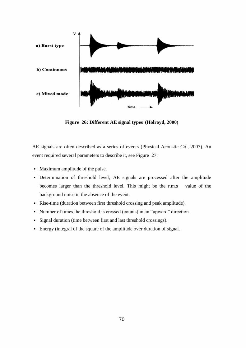
70
Figure 26: Different AE signal types (Holroyd, 2000)
AE signals are often described as a series of events (Physical Acoustic Co., 2007). An
event required several parameters to describe it, see Figure 27:
Maximum amplitude of the pulse.
Determination of threshold level; AE signals are processed after the amplitude
becomes larger than the threshold level. This might be the r.m.s value of the
background noise in the absence of the event.
Rise-time (duration between first threshold crossing and peak amplitude).
Number of times the threshold is crossed (counts) in an “upward” direction.
Signal duration (time between first and last threshold crossings).
Energy (integral of the square of the amplitude over duration of signal.

71
Figure 27: The typical AE signal features (Physical Acoustic Co., 2007)
Wear Conditions and Acoustic Emission 4.8
Various methods have been used to detect and diagnose fatigue in rolling contact in
bearings, and AE is the latest. However, the results still have not been completely
successful because the AE measurement techniques developed thus far have dealt only
with the AE emission generated by rolling contact with time. (Tekeo and Takashi, 1982)
have shown that by employing of acoustic emission technology it could be explored
defects of rolling bearings before the start of accelerated vibration . There is needed to
further clarify the type of relationship between AE and wear failure (Halme and
Andersson, 2010; Mba, 2003). After studying the relation between AE and failure
detection in rolling contact fatigue processes it was clear that the AE was related to
bearing fatigue failure and can precisely locate the defect position.
(Sarychev and Shchavelin, 1991) investigated the relationship between cumulative AE
counts and frictional work, it was found that the real area of contact between surfaces
comprised a number of discrete asperity contacts and the deformations of these are
associated with the AE output with only larger asperities generating AE above the
threshold level. In dry sliding metals it was easy to detect the AE signals which were
varied more or less consistently with process conditions (speed and load) and material

72
combination used. (Lingard and Ng, 1989)found there was an increase in the cumulative
AE counts with total friction work. Also the rate of AE was directly proportional to the
contact area in the direction of sliding.
A ball and cylinder test rig give conditions of pure sliding if a stationary ball is held
against a rotating cylinder. (Boness et al., 1990) postulated that the first peak in the r.m.s
value of the signal was associated with the initial removal and gross deformation of the
original surface asperities. A special test using a polished cylinder established that when a
full elastohydrodynamic film existed between the specimens no r.m.s signal above the
noise level of the instrument could be detected, inferring that asperity contact was the
prime source of the AE signal.
A scanning electron microscope (SEM) examination of the rubbing surfaces showed that
the gradual increase to the second peak in the r.m.s value of the signal was related to
transference of debris from the rotating cylinder to the smoother stationary ball. For the
unlubricated situation the erratic behaviour of the r.m.s signal after 120 s was observed
to be predominantly due to abrasive wear. It was demonstrated that r.m.s measurements
of the AE signals provide a valuable tool in the study of wear between dry and lubricated
sliding contacts. The time-dependent nature of the r.m.s signal is able to distinguish
between different wear mechanisms. A direct empirical relationship between integrated
r.m.s signal and the wear volume removed from the test ball in a ball on cylinder test rig
was obtained (Boness et al., 1990).
(Mechefske et al., 2002) studies the mild-to-severe wear transition using sapphire sliding
over steel sliding disks using AE to measure changes in test conditions. AE signals
generated during the wear process were analysed in both time domain and frequency
domain. Experiments demonstrated that AE has the possibility to be a useful wear rate
monitoring technique. In the time domain the increase of AE r.m.s and peak level values
were in direct proportion to the sliding speed and inversely proportional to the applied
load conditions and so are useful measures of the wear surface strain rate.
Boness et al [60] indicated that the asperity contact, micro-crack initiation and growth,
plastic deformation are the basic wear mechanisms. Also, Boness et al stated that the AE
signature was mostly continuous with superimposed AE burst attributed by the rapid
high-amplitude at events the rubbing surfaces. Boness at al [60] experienced AE under

73
dry and lubricated contacts under pure sliding conditions. Tests with a full
elastohydrodynamic film between highly polished surfaces did not generate any AE
activity above the electronic noise of the acquisition system, inferring that asperity
contact was the prime source for AE. Also found AE r.m.s signal varied directly with
wear Volume. In general, the occurrence of severe wear results in high AE activity as
evidenced by a high AE count rate in the time domain and high spectral variation in the
frequency domain (Boness et al., 1990; Jiaa and Dornfeld, 1990).
(Tan and Mba, 2005b) investigated the use of AE detection of pitting damages on gear
teeth surfaces. They noticed that the lubricant oil temperature is relatively higher at
higher operating torques generating a higher r.m.s value in the AE signal, of course at
this higher temperature the oil film is thinner resulting in more asperity contact so long as
the lubricating regime is under partial EHL. They concluded that a linear relationship
existed between measured AE levels generated by pitting of a gear pinion and area of
pitting and that detection of pitting began when only 8% of the area was pitted. This
strongly suggests that AE techniques can be used for health monitoring and pit
progression. It was also found that AE offered better sensitivity to pitting progression
from the bearing casing than the vibration method, depending on load conditions
(Vincent, 2007).
Detection of incipient faults in rolling element bearings at low speeds was evaluated
experimentally by (Eric Y et al., 2007) it was found the time domain r.m.s value was the
best parameter to clearly show the difference between normal and defective bearings
regardless of speed and type of the defect.
Preliminary fatigue testing of a complete landing gear has demonstrated the applicability
of the AE signal using resonant sensors attached to the outer surface of the landing gear
assembly. Fatigue crack monitoring of compact test specimens has confirmed that AE can
detect the initial stages of crack growth in typical landing gear materials (Matthew G et
al., 2004). The study examined AE from fatigue cracks in compact tension specimens
using a broadband transducer and a resonant sensor to assess their effectiveness in
monitoring fatigue crack growth in aerospace grade steel. It was shown that detection of
fatigue crack growth in aerospace grade steel compact tension specimens using
appropriate AE techniques is possible. Furthermore a quick and efficient way to

74
distinguish between emissions from a hydraulic actuator and fatigue crack growth in the
laboratory has been identified (Matthew G et al., 2004).
Gear faults monitoring using acoustic emission. 4.9
(Boness et al., 1990; Boness and McBride, 1991) investigated the application of AE to
both sliding and rolling conditions and found that asperity contact generated AE. This
research was an attempt to better the understanding of how the operation of both helical
and spur gears generate AE. That work was extended by (Tan and Mba, 2005b;
Toutountzakis et al., 2005) who found that the principal AE sources are interactions
between the surface roughnesses of the two gears due to their relative motion. Helical and
spur gears undergo combined rolling and sliding on both sides of the pitch point, and pure
rolling at the pitch point. However, due to the geometry of the helical gears, the pitch
point during gear mesh does not pass along the width of the gear at the same time as with
meshing of spur gears mesh, instead pitch point contact for the helical gear mesh is
progressive.
The operating life of gears is determined by the lambda ratio which is vital for
maintaining mechanical integrity. Recommended values for have been published but
the actual value is difficult to determine during operation. EHL studies have shown that
is predominantly determined by temperature, load, surface roughness and speed of the
meshing gears (Dowson, 1977; Dowson, 1995). Because changes with change in any or
all these parameters, the level of contact between the surface asperities during gear
meshing will also vary.
(Hamzah and Mba, 2009) observed that AE was more sensitive to changes in specific
film thickness under combined rolling and sliding (spur gear) compared to pure rolling
(helical gear).and established a relationship between load, speed and AE for both spur
and helical gears; the increase in speed increases the AE r.m.s and the reduction in load
conditions, has reduced the AE r.m.s . levels. Further the variation in AE levels during
helical gear mesh is suggested as attributable to not only the asperity levels but also to the
variation in contact length during meshing.

75
Acoustic Emission Activities Constraints 4.10
(Loutas and Kalaitzoglou, 2007) compared the abilities of monitoring techniques to
differentiate between different load and defect states in a single stage gearbox. It was
observed that the AE r.m.s changed with increasing oil temperature and these findings
confirm the conclusions of (Tan et al., 2007) and (Toutountzakis et al., 2005) that oil
temperature significantly affected AE and should always be taken into account.
Pitting in gear tooth progresses from of micro-cracks initiation and crack growth to the
separation of tiny particles from the gear surface. Simultaneously, these particles and
other debris resulting from wear create abrasions between teeth surfaces. All these stages
emit AE.
The detection of defects seeded into gearboxes using AE is fraught with difficulties. The
biggest burst of the AE signals were not always present in the centre region of the
window at the same location as the artificial fault (pit) on gear tooth. However, some
researchers claim to have shown the contrary; that the AE energy as measured by the time
domain r.m.s clearly distinguished a simulated pit, micro-cracks initiation and crack
growth up to removal of tiny particles from the gear surface (Tandon and Choudhury,
1999; Toutountzakis and Mba, 2003). In addition third-body abrasions will be created by
wear particles removed from gear surfaces and will have their own AE activity and
further complicate observations (Matthew G et al., 2004). As stated earlier AE levels are
inversely proportional to oil film thickness and directly proportional to asperity contact
and are influenced by surface roughness (Tan and Mba, 2005b; Ebersbach et al., 2006).
Acoustic Emission and lubricant 4.11
(Benabdallah and Aguilar, 2008) investigate how the AE depended on friction and wear
properties using a ball-on-cylinder lubrication test machine with a fixed, stationary ball
sliding over a flat ring around a rotating cylinder. Included in the investigation was dry
sliding contact lubricated with pure grease and contamination simulated by the
introduction of small glass particles. The speed of the cylinder (sliding speed of the ball)
was the parameter of major interest and it was found that for dry contact: sliding contact

76
generated a continuous AE waveform, the r.m.s voltage of the AE signal produced by
the ball sliding over the ring was a good measure of the coefficient of friction (µ).
(Jie and Drinkwater, 2006) used an ultrasonic technique to measure the thickness of
lubricating films for the rolling element of a ball bearing steel type 6016. The results
obtained were in good agreement with those produced by EHL theory over the range 0.3–
1.0 μm for radial loads greater than 2.5 kN but shaft speeds were limited to less than 200
rpm (3.3 Hz). Ultrasonic measurements suffer from a number of limitations, including:
the pulse repetition rate limits the number of measurement points, the ultrasonic beam
does not focus at a point but over a small area and so gives an average value over that
area. However it was clearly demonstrated that ultrasonic measurement has the potential
for monitoring the thickness of lubricant films in industrial applications.
(Toutountzakis et al., 2005; Toutountzakis and Mba, 2003) used AE for an experimental
investigation of gear defects and their diagnosis. They showed that AE monitoring of the
health of gears was a useful tool that would allow monitoring for developing defects in
gears externally, from a sensor on the bearing casing. (Tan and Mba, 2005a) noted that
for isothermal conditions the imposed load had a minimal effect on the r.m.s level of the
AE signal, but that speed had a significant effect. They confirmed that for rolling contact
the level of the AE signals depended on the speed of rotation of the gears and that AE
transients were found at the gear mesh frequency. The r.m.s value of the AE signal also
depended on film thickness. The relative proportions of rolling and sliding contact
strongly affected the overall level of the AE signal.
(Hamzah and Mba, 2007) extended previous work into the generation of AE as a function
of using helical and spur gears made of 045M15 steel without any heat treatment, in a
standard back-to-back oil bath lubricated gearbox, powered by a 1.1 kW motor. It was
found that the value of clearly and directly influenced the level of the AE signal for
both types of gears (inversely proportional).
(Eftekharnejad and Mba, 2008; Eftekharnejad and Mba, 2009) assessed the ability of AE
to identify specific defects seeded into helical (214M15) steel test gears. The gearbox test
rig used was the same back-to-back arrangement as used by (Hamzah and Mba, 2007). It
was operated at a speed of 11.5 Hz (690 rpm). Mobilgear 636 oil was the lubricant used.
They concluded that the AE waveform could be used to identify the seeded defects. They

77
also concluded that the measured AE r.m.s levels were more useful for identifying the
seeded faults than vibration measurement made with an accelerometer situated on the
bearing pedestal. However (Toutountzakis and Mba, 2003; Hamzah et al., 2008) using a
similar test procedure found this was not the case for spur gears.
In most of the studies conducted earlier, the impact of specific film thickness (λ) or rather
lubrication regime on the AE generation has at gear contact area not been investigated in
detail. And the main focus of previously published work was on the use of the AE
technology for the detection of defects on gear tooth surface, and understanding the
influence of the operation parameters such as applied load, speed, and surface roughness
on the AE signal.
Thus the aim of this project work is to understand how three different lubricating
conditions, hydrodynamic (HL), elastohydrodynamic (EHL) and boundary (BL)
lubrication influenced the generation of AE at the meshing gears. Gear operating
temperature will be changed while whilst AE activity in monitored during the whole test.
The main objective of this research programme is to assess the potential of AE
technology as a monitoring tool capable not only to detect the failure onset but as an
effective preventive maintenance tool. Knowing the lubrication regime at gear meshing is
responsible on lubrication-related-failures. So, in this research programme, the capability
of AE in quantifying the lubrication regime of the operational helical gears will be
evaluated.

78
Chapter 5
Experimental Setup
and procedure

79
5 Experimental Setup and procedure
Experimental Gearbox 5.1
The test programme used a back-to-back type gearbox designed and fabricated at
Cranfield University comprising slave gears driving the test gears via a flexible coupling,
see Figure s 28 and 29. This type of gearbox is typical of those used for gear fatigue tests
(Vayionas, 1991). AC 3 phase 1KW electric motor was used to drive the gearbox. A
flexible coupling connected the motor input to the slave gears, two loaded plates on the
power return shaft were used to dissipate the energy of the motor. The loading coupling
consists of couple of half flanges bolted to each other; through a threaded hole on one of
the flanges. The applied torque rotated the loaded plates against each other (Vayionas,
1991). The idea of applying the back-to-back arrangement is to allow the torque to be
maintained within a closed loop so that the power requirement overcomes frictional
losses only. In other words, when the gearbox is operating at a steady speed, even when
the test gears are operated under very high load, the energy supplied by the drive driving
only has to compensate for power losses in the system.
Figure 28: Back-to-back gearbox
Slip-ring
Electric motor (1KW)
Slave Gears Test Gears F-Coupling
Loading Plates

80
The details of the gearbox design are presented schematically in Figure 29.
Figure 29: Schematic diagram of the test arrangement
V acce
lerom
eter
A
E senso
r
Th
ermo
cou
ples

81
5.1.1 Gears
The helical gears from HPC Gears Limited were used for the experiment. These were
045M15 steel supplied without any heat or surface treatment. The pinion (or driver gear)
had 51 teeth and wheel (or driven gear) had 70 teeth. The contact ratio was 1.7 mm and
center distance between the pinion and wheel was 171 mm. A 25 mm face width was
used for both pinion and wheel during the tests. Table 3 shows the gear specifications.
Table 3: Specifications of helical gears used in the experimental work (Appendix A)
Specification of test gears
Pinion Wheel
Number of teeth 51 70
Module 3 mm 3 mm
Pressure angle 20 20
Helix angle 17.5 17.5
Contact ratio 1.7 1.7
Face width 25 mm 25 mm
Direction Right Hand Left Hand
Hardness 137 Hv30 137 Hv30
Surface roughness 1.327 μm 1.327 μm
Pitch circle diameter 160 mm 220 mm
Size of Addendum 3 mm 3 mm
Size of Dedendum 3.75 mm 3.75 mm
5.1.2 Electrical Motor
A 1 kW AC electrical motor of operating speed 690 rpm was used to power the back-to-
back gearbox. The operating speed was measured using a tachometer at the input shaft;
the accuracy of the measurements was ±1 rpm.

82
5.1.3 Lubrication
Splash lubrication was used for the gears during the tests. This is supported by (Drago,
1988.) who claims that splash lubrication is well suited to applications with pitch line
velocity less than 25.4 m/s. The pitch line velocity used in these tests was approximately
5.4 m/s which is well below the Drago limit. Mobilegear 636, a high performance oil
intended for splash lubrication in gearboxes was used, see Table 4.
Table 4: Specification of the lubricant (Appendix C)
Lubricant properties Mobil gear 632
Kinematics viscosity at 40 C˚ 664 (cSt)
Kinematics viscosity at 100 C˚ 62.8 (cSt)
Viscosity index ASTM D2270 165
Density at 15_ ASTM D4052 0.87
5.1.4 Loading Plates
The back-to-back gearbox arrangement is to contain the torque inside a closed loop
system so that ay a steady operating speed the power requirement overcomes frictional
losses only (Vayionas, 1991) and (Hamzah and Mba, 2007). The maximum applied
torque in this system is 370Nm with an accuracy of + 5Nm. Twisting the loading plates
against each other by tightening or loosening a bolt into or out of the threaded hole. This
procedure will allow a static torque to be applied across the gearbox, see Figure 30. The
loading plate consists of two half flanges bolted to each other; one of the flanges has a
threaded hole. The loading plates were calibrated using an optical strain gauge with
rosette arrangement mounted at the opposite shaft connecting slave and test pinions
together.

83
Figure 30: Loading plates
5.1.5 AE Sensors
Physical Acoustic Corporation (PAC) Acoustic Emission wideband (WD, Physical
Acoustic Corporation) sensors (with operating frequency range from 100 KHz to 1 MHz
were used for the test work. The AE sensors were mounted on the pinion and held in
place with superglue.
5.1.6 Thermocouples
K-type (Iron-Constantan) thermocouples - see Table 5 for brief specifications - were used
to measure gear metal and lubricant temperatures. Five thermocouples were mounted on
the test pinion and one dipped into the lubricant (RS Components Ltd, UK). J-type
thermocouple was used and placed inside the oil bath for monitoring oil temperature.
Table 5: K&J-type Thermocouple Specification (Appendix D for data sheet)
Maximum Temperature Sensed +200°C
Minimum Temperature Sensed 0°C
Probe Diameter 6.35mm
Probe Length 1000mm
2 Flanges of
Loading Plate

84
5.1.7 Slip Ring
A Moog Components PM-12 80039-950 slip ring with 12 contact channels was used - see
Appendix E for specifications. The slip ring was used to transmit the signals from the AE
sensor mounted on the pinion to the data acquisition board. Figure s 28, 29 and 31 show
the slip ring connected in-line with the input shaft of the gearboxes at the end of the test
gearbox.
Figure 31: Slip ring
5.1.8 Pre-Amplifier
AE piezoelectric transducers are high impedance sources producing low voltage signals
and so require both pre-amplifier and amplifier. A PAC preamplifier made by the
‘Physical Acoustics Corporation) was used this has gain settings of 20, 40 and 60 dB. It
also has a plug-in filter and single-ended and differential sensor inputs. The AE output
signal was fed directly from the pre-amplifier to the data acquisition card using BNC
connectors on coaxial cable.
Slip ring Rubber connector
Pinion shaft

85
5.1.9 Accelerometers
The accelerometer used for vibration measurement in this experimental work was an
Endevco Dynamic Instrument Division ISOBASE Model 236 piezoelectric transducer
with operating frequency between 10 and 8000 Hz. One of the accelerometers was
mounted on the pinion shaft bearing pedestal and the second was mounted on gear casing,
see Figure 39, to record the vibration of the gear system at that point.
.
Data Acquisition (DAQ) Cards 5.2
A Physical Acoustics Corporation PAC PCI-2 16-bit, two channel card was used to
continuously acquire the AE signal, from which such parameters as the r.m.s level,
Absolute Energy and Absolute Signal Level (ASL) were obtained. The card has a
maximum sampling rate of 5 MHz. The system has anti-aliasing filters prior to the
Analogue to Digital Converter (ADC) which can be controlled directly from the software.
For higher speed data capture a Physical Acoustics Corporation MISTRAS AE DSP-
32/16 16 bit 2 channel card with a maximum sampling rate of 10 MHz was used.
5.2.1 Data Acquisition (DAQ) Software
AE-win
AE-win Version E1.62 software developed by the Physical Acoustics Corporation was
used to calculate and record the r.m.s , Absolute Energy and ASL of the AE signal. With
this package real time calculation of the AE parameters is possible. Each value from the
ADC was squared and added into the accumulator by a “hardware accelerator” for the
programmed time interval. The r.m.s value was found by taking the square root of the
accumulated squared ADC readings. For real time calculations the software has the
minimum time driven rate of 10 milliseconds and minimum time constant of 10
milliseconds. The accumulator was cleared at the end of each time interval and then the
same process was repeated. The software is capable of recording the waveform at a
maximum sampling rate of 5 MHz.

86
Mi-Tra
With the MISTRAS AE DSP-32/16 card the software used acquire the AE raw waveform
data was Mi-Tra Mistras 2001 E1.73. This package has a digital filter of between 10 kHz
to 1200 kHz. The pre-amplifier range that the software can accommodate is between 0 dB
and 60 dB. The test arrangements are shown schematically in Figure 33.
Lab-view 7.5 software script was used for temperature measurements and display.
Instrumentations
AE Sensors Thermocouples
Slip ring K-type(gear) J-type (Oil)
slip ring
Pre-amplifier Data acquisition cards
Trigger sensor Lab-view software
Charge amplifier
Data acquisition cards
AE Software Waveform software
Figure 32: Schematic diagram of the Data Acquisition Systems
Experimental Procedure 5.3
The research was undertaken with Mobilgear 636 lubrication on the helical gear. A load
of 370 Nm was used at this stage of the test procedure. Gear data, lubricant properties and
operating conditions were as shown in tables 3 and 4.
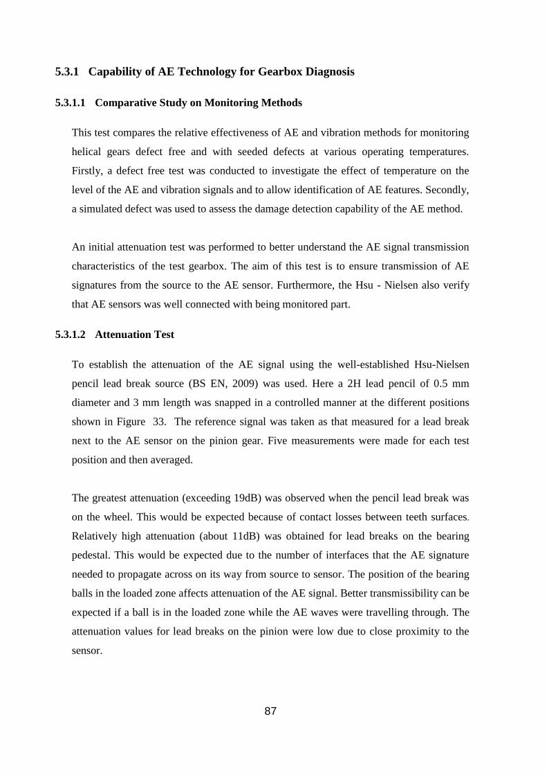
87
5.3.1 Capability of AE Technology for Gearbox Diagnosis
5.3.1.1 Comparative Study on Monitoring Methods
This test compares the relative effectiveness of AE and vibration methods for monitoring
helical gears defect free and with seeded defects at various operating temperatures.
Firstly, a defect free test was conducted to investigate the effect of temperature on the
level of the AE and vibration signals and to allow identification of AE features. Secondly,
a simulated defect was used to assess the damage detection capability of the AE method.
An initial attenuation test was performed to better understand the AE signal transmission
characteristics of the test gearbox. The aim of this test is to ensure transmission of AE
signatures from the source to the AE sensor. Furthermore, the Hsu - Nielsen also verify
that AE sensors was well connected with being monitored part.
5.3.1.2 Attenuation Test
To establish the attenuation of the AE signal using the well-established Hsu-Nielsen
pencil lead break source (BS EN, 2009) was used. Here a 2H lead pencil of 0.5 mm
diameter and 3 mm length was snapped in a controlled manner at the different positions
shown in Figure 33. The reference signal was taken as that measured for a lead break
next to the AE sensor on the pinion gear. Five measurements were made for each test
position and then averaged.
The greatest attenuation (exceeding 19dB) was observed when the pencil lead break was
on the wheel. This would be expected because of contact losses between teeth surfaces.
Relatively high attenuation (about 11dB) was obtained for lead breaks on the bearing
pedestal. This would be expected due to the number of interfaces that the AE signature
needed to propagate across on its way from source to sensor. The position of the bearing
balls in the loaded zone affects attenuation of the AE signal. Better transmissibility can be
expected if a ball is in the loaded zone while the AE waves were travelling through. The
attenuation values for lead breaks on the pinion were low due to close proximity to the
sensor.

88
Figure 33: Schematic diagram showing the different test positions at which the
Nielsen source was located
5.3.1.3 Seeded Defect for First Test
For the seeded defect test, a pitch line defect was introduced onto a single tooth as a deep
rectangular scratch (8 mm long x 3 mm wide x 2 mm deep) as shown in Figure 34. The
gearbox was then restarted and the same measurement procedure followed as for the
defect free test.

89
Figure 34: Seeded defect on single tooth
5.3.2 Influence of Lubrication Film Conditions on AE Signal
The purpose of this test was to study the effect of temperature of the lubrication on the
AE signal. This could be achieved only using wide range of temperatures, which required
the use of liquid nitrogen to cool gear system and thus give a wide range of lubrication
film thickness.
This test was performed to better understand the influence of temperature variation on the
behaviour of specific film thickness (λ) and resulting generation of AE activities. The
assumption is that lubricant viscosity is affected by temperature which thus has a direct
influence on type of lubrication regime and specific film thickness (λ) generated during
gear meshing (Dowson, 1977).
Liquid nitrogen was used to obtain a large temperature drop (up to 10C per minute).
Figure s 35 and 36 show the location and manner in which the liquid nitrogen was
sprayed onto the gear wheel. The wheel was chosen as the location because AE signals
generated here suffered maximum attenuation and so any macro- and/or micro-structural
activity of the gear material due to rapid reduction in temperature during the test would
Seeded defect

90
be minimal at the sensor. Gear temperatures were reduced by spraying liquid nitrogen at
the cylider pressure of 2 bars through the nitrogen gun made an angle of 45o with the
wheel surface. The tip was placed as close as possible to the wheel (approximately 5
mm), see Figure 36. (Hamzah et al., 2008) has demonstrated this is necessary to avoid
freezing the oil mist and forming oil crystals which generates unwanted AE activity when
crushed inside the gear mesh.
Figure 35: Cooling arrangement showing nitrogen gun nozzle
Figure 36: Liquid nitrogen gun location and gear wheel
Nitrogen Inlet
Nitrogen gun distance between
the tip and wheel is 5mm
Wheel gear
Pinion gear
Gearbox Cover
Nitrogen gun

91
And this is the brief View of testing methods:
5.3.2.1 Influence of Temperature Variation on AE Activity
The gearbox was run until the temperature stabilized at about 43°C (with a change of no
more than ±1°C over an hour). The gearbox ran for a total time of about 4 hours at
370Nm load and speed 690 rpm. To remove heat and reduce the temperature, liquid
nitrogen was spraying, approximately at rate of 10˚C per minute, onto the wheel through
a 5 mm diameter steel pipe, see Figure 37. After about 10 minutes and when the
thermocouple on the pinion recorded a temperature of 0oC, the supply of nitrogen was
stopped. The gearbox was then run continuously during which time the temperature
increased until it was at about the same level as when the nitrogen flow commenced. This
procedure was repeated three times to reduce random errors and ensure more accurate
results.
5.3.2.2 Diagnosis During Dry and Lubricated Contact
To obtain dry contact for the start of the test the lubricating oil was sucked out of the
gearbox using suctions pump, and it was run dry for about five minutes. Oil was then
injected into the gearbox, the gearbox was running, which continued to run until both the
gear and lubricant oil reached a steady temperature (40°C), After that test followed same
procedure as described in previous test.
5.3.2.3 Defective Gear Diagnosis During Dry and Lubricated Contact
To investigate the effect of oil regimes on defect detection using AE signals a defective
gear was used, see Figure 37. The test followed same procedure as described above.

92
Figure 37: Defective gear
Figure 38 shows a schematic diagram of the experimental procedure and Table 6 shows
the tests carried out in this project.
Defects

93
Figure 38: Schematic diagram of the experimental procedure
Table 6: Experimental stages
Process
Dry run
Oiling run Till stabilization of
temperature
Cooling run using nitrogen till
0°C
Warming up
1
Comparative test
First test
3 Influence of oil film on AE
Second test, Third test and Fourth test
comparative test
AE sensors
Pinion & Case
Vibration accelerometer
pedestal & Case
Normal Seeded defect
Influence of oil film on AE test
Normal gear lubricated gears
test
Normal gear dry & lubricated
gears test
Defective gear dry & lubricated
gears test

94
Chapter 6
Results and
Discussion

95
6 Results and Discussion
Capability of AE Technology for Gearbox Diagnosis 6.1
Comparing AE activity from defect free and simulated defect conditions under varying
loads and/or speeds can be very misleading if the effect of oil temperature is not
considered. Previous studies related to gearbox diagnosis with AE have shown that the oil
temperature affects the AE signal because lubricant temperature is an influential factor in
AE generation (Tan and Mba, 2005a; Hamzah et al., 2008). These changes in the AE
activity due to change in oil temperature have significant consequences that require more
research work to develop AE as a robust diagnosis tool that includes temperature effects
and so reduce errors.
6.1.1 Test Instrumentation and Procedure
Two wide-band AE sensors were used throughout the tests. One sensor was placed on the
pinion (first channel) and the other on the gearbox casing (second channel) as shown in
Figure 39. The cable connecting the sensor placed on the pinion with the pre-amplifier
was fed into the shaft and connected to a slip ring placed at the end of test gearbox. This
arrangement allowed the AE sensor to be placed as close as possible to the gear teeth.
Both sensors were held in place using super glue. AE signals were pre-amplified at 60 dB
for both sensors. A PH-12 slip rig manufactured by ‘IDM Electronics Ltd’ was used. The
slip ring used silver contacts and could accommodate up to 12 channels. AE sensors were
of differential type with a relative flat response of between 100 kHz and 1 MHz. AE was
recorded with MISTRAS AE DSP-32/16 data acquisition card at a sampling rate of 5
MHz. Accelerometers (ISOBASE 236 Endevco) used had an operating range of between
10 Hz and 8 kHz.
Figure 39 shows the way the accelerometers were mounted, one mounted on the bearing
pedestal of test gear and the other on the gearbox casing. All vibration data was recorded
at a sampling rate of 10 kHz. J-type thermocouple, rated from -60 C° to +850 C° was
placed inside the oil bath to monitor the temperature during the experiment see Figure
37. It was important that any data recorded was taken from a well-defined

96
circumferential point at every revolution because this experiment focused on assessing
the applicability of AE for identifying seeded defects on helical gears. For this reason, an
optical triggering mechanism was used. The triggering system consisted of metal disk
with 2 mm diameter hole and an optical sensor. Each time the hole passed through the
optical sensor the AE and vibration acquisition systems were triggered.
An Analogue-to-digital converter (ADC) controlling software was used to calculate
continuous AE r.m.s values in real time. The hardware accelerator used by the software
enabled the calculations of the AE r.m.s in real time. Each value from the ADC was
squared and added into the accumulator by the hardware accelerator for a programmable
time interval, 90ms in this case which corresponds to very slightly below one complete
revolution of the pinion at the rotational speed (690 rpm). To calculate the r.m.s , the
square root of the accumulated squared ADC readings was used. The accumulator was
reset at the start of each new time interval and the same process was repeated. The time
interval for the acquisition was set at 90 ms.
Figure 39: AE and vibration sensors locations
The defect free gearbox was run at a given load and speed (370 Nm and 690 rpm
respectively) for a period of 5 hours so that the gearbox reached a stable temperature. The
acquisition time window of 16 teeth was set for which the trigger mechanism allowed an
acquisition duration of 0.0256-s, which corresponds to 16 teeth at 690 rpm for each set of
Accelerometers
AE sensors Thermocouple of
oil bath

97
data. At the beginning of the test, when the oil was still at room temperature, a defect free
recording of AE and vibration was undertaken. The instantaneous recording was made to
allow the influence of temperature on the levels of AE and vibration to be investigated.
The AE and vibration signals were then recorded with the gearbox running at each 3oC
rise in temperature of the oil bath until the temperature stabilized at 54oC. To check
repeatability, the tests were carried out twice. In order to introduce the seeded defect, the
test rig was stopped and the defect introduced, see Figure 34. The gearbox was then
restarted and the same procedure was followed for the seeded defect run.
6.1.2 Results Based on Acoustic Emission AE Monitoring
The AE sensors on the pinion and gearbox casing were synchronized, so that when the
data acquisition system was triggered, both AE sensors captured data simultaneously.
Figure 40 shows typical waveforms for the defect free condition at 370 Nm. Continuous
type AE waveform is dominant although transient AE bursts whose amplitude
considerably exceeds the underlying continuous wave can be seen (Don’t forget a
“continuous” AE waveform is a series of bursts of similar amplitudes so close together
that they cannot be separated). The frequency of the periodicity of these AE bursts
represents the number of meshing teeth within the acquisition window. This is similar to
the observations of (Tan and Mba, 2005a) who studied AE waveforms in spur gear
meshing in which both continuous and transient type fo r.m.s of AE activity were
apparent. Tan and Mba concluded that rolling contact on the pitch line of the spur gear
mesh was responsible for generating high amplitude AE transient bursts, whilst sliding
contact generated a large portion of the continuous waveform. In the case of the helical
gears, contact between a specific gear pair begins as a minute contact point which
increases in contact length as the pair engage while decreasing contact length occurs as
the pair disengage. The contact length varies along the pitch line of the helical gears but
in spur gears the contact length remains constant. Furthermore, the continued variation in
the contact length during meshing of helical gears directly influences the load conditions
experienced by the gear and leads to instantaneous changes in oil film thickness (Hamzah
and Mba, 2007). Thus, AE waveforms associated with helical gear meshing are expected
to be of the continuous type with amplitude variations attributed to the gear mesh length,
see Figure 40.

98
Figure 40: AE waveform associated with a defect free condition
Typical AE waveform associated with defected tooth is shown in Figure 41. The
relatively large transient AE bursts associated with tooth meshing are clearly seen over
the continuous AE levels. The transient AE bursts were observed to originate in the
region of the tooth where the defect was seeded. Such observations were not observed in
a similar test with spur gears; that means the seeded defects were not evident in the
waveforms (Toutountzakis and Mba, 2003; Tan and Mba, 2005)
Figure 41: AE waveform associated with a tooth defect
0 0.5 1 1.5 2 2.5 3
x 105
-0.4
-0.3
-0.2
-0.1
0
0.1
0.2
0.3
0 0.005 0.01 0.015 0.02 0.025 0.03-0.8
-0.6
-0.4
-0.2
0
0.2
0.4
0.6
Time(s)
Ampli
tude(v
olts)
Defective tooth
0 0.005 0.01 0.015 0.02 0.025 0.03-0.8
-0.6
-0.4
-0.2
0
0.2
0.4
0.6
Time(s)
Am
plit
ude(v
olts)

99
The variation in the oil temperature with the operating time is shown in Figure 42. It is
clear that there was no significant difference in oil temperature between the fault free and
seeded defect conditions. Thus AE data was for the two conditions was acquired at the
same temperatures.
Figure 42: Oil temperature with time; defect free and with seeded defect
In both the cases, the oil temperature increased at a faster rate in the first hour after which
the rate of increase reduced. Note that it took the gearbox system at least 5 hours of
continuous running to reach a stable temperature.
Figure 43 shows the r.m.s value of the AE signals with temperature for both channels.
For the AE sensor placed on the pinion (first channel) it can be seen that the AE r.m.s
levels with the seeded defect increased as the oil temperature increased. In the defect free
test it was noted that the AE r.m.s value for the sensor on the opinion grew at the start of
test resulted to increase in oil temperature, this increase enabled the increase in asperities
contact, and when oil thermal stabilised led to the stability in AE r.m.s .
0
10
20
30
40
50
60
0 60 120 180 240 300
Tem
per
ature
C°
Time(mins)
Free defect run seeded defect run

100
The increase in AE r.m.s was progressive in seeded-defect case. This trend of AE r.m.s
with oil temperature shows the presence of the simulated defect in the gear tooth. This
increase in AE r.m.s was attributed to pinion tooth defect contact with wheel teeth due
to decrease in oil film thickness in the contact area.
The AE r.m.s levels measured by the sensor on the gearbox casing (second channel) did
not vary with temperature in the same manner as noted with the sensor on the pinion.
This is due to dissipation and attenuation of the signal during transmission before it was
received by this sensor.
The relation between AE absolute energy and oil temperature for both AE signals
channels for both free/seeded defect tests are shown in Figure 44. As expected the AE
energy for the first channel increased with the oil temperature in the case where the
seeded defect was present and, again, no specific trend was seen with the second channel.
Figure 43: AE r.m.s values at each sensor with oil temperature
0
1
2
3
4
5
6
7
8
9
10
27 30 33 36 39 42 45 48 51 54
AE
r.
m.s
(m
v)
Temperature C
defect free- first channel defect free-second channel
seeded defect-first channel seeded defect- second channel

101
Figure 44: AE Energy values at each sensor with oil temperature
The Kurtosis (KURT) and Crest Factor (CF) of the AE signals are shown in Figure 46a
and 46b, respectively with and without the seeded fault and with change in oil
temperature (first channel). Both K and CF are measures of the peaks in the spectrum and
would be expected to increase with the seeding of the defect. From Figure 46a it can be
seen that the K value for the defect free test shows very little variation with temperature.
However, the K value when the seeded defect is present shows a clear ascending trend,
especially above an oil temperature of 36oC. This was attributed to the increase of oil
temperatures giving a decrease in the oil viscosity led to the decrease in the oil film
thickness in contact area of the gear mesh.
Similar trends are observed with the CF, see Figure 46b. At lower oil temperatures CF
and K values are not significantly different but above 36oC the CF shows a clear
indication of the presence of a defect.
0.00E+00
1.00E+04
2.00E+04
3.00E+04
4.00E+04
5.00E+04
6.00E+04
7.00E+04
8.00E+04
9.00E+04
27 30 33 36 39 42 45 48 51 54
AE
-Ener
gy(J
)
Temperature C°
Seeded defect run gear sensor Seeded defect run case sensor
Free defect run gear sensor Free defect run case sensor

102
It was concluded that both Kurtosis and Crest Factor provided an upward trend with oil
temperature reflecting the presence of a fault and thinning of the oil film under a fixed
load and speed conditions.
Figure 45: Statistical parameters of the AE first channel signals, a) kurtosis and b)
Crest Factor.
0
5
10
15
20
25
30
35
40
45
27 30 33 36 45 48 51 54
Ku
rto
sis
Temperature (c)
KURT--Seeded Defect run
KURT--Non Defect run
a)
0
5
10
15
20
25
30
27 30 33 36 45 48 51 54
Cre
st F
acto
r
Temperature(c)
CF-Non DefectD run
CF-Seeded Defect run
b)

103
It can be concluded from the results presented here that for constant speed and load,
increasing oil temperature in the gear system or introducing a tooth fault had negligible
effect on vibration r.m.s as measured at both the bearing pedestal and gearbox case.
The AE measurements made by the sensor on the gearbox casing also showed no
significant change with seeded defect or change in oil temperature. This was attributed to
high attenuation of AE signal before reached the sensor.
However, for the sensor on the gear, increasing oil temperature with the seeded fault had
a considerable effect on Kurtosis and Crest Factor. Above 36oC both these statistical
measures gave a strong and positive indication of the presence of a defect.
Influence of Lubrication Film Conditions on AE 6.2
6.2.1 Test Instrumentation and Procedure
The AE sensor was placed near to the tooth root of the pinion gear as shown in Figure
47.
Figure 46: Locations of the AE sensor and thermocouples
This test involved observing AE generation levels under elastichydrodynamic (EHL) and
hydrodynamic (HL) conditions.
Prior to the start of this test the gearbox was run for a period of 4 hours at 370 Nm load
and a speed of 690 rpm until the temperature reached thermal balance, in this test was
AE sensor
Thermocouples

104
about 43°C (-/+ 1°C). The liquid nitrogen was sprayed onto the rotating wheel gear
through angled pipe so that no nitrogen directly impinged on the meshing area. While the
nitrogen liquid was being sprayed on to the wheel, the temperature and AE r.m.s was
measured in real-time, and AE waveforms were captured at different instances during the
test. The flow of liquid nitrogen was halted when the temperature of the metal of the gear
reached 0°C. After the supply of nitrogen was stopped the gearbox was allowed to
continue operating hence the temperature of the lubricant increased gradually to about the
same level as before the liquid nitrogen was introduced.
The AE r.m.s was measured and recorded in real time with a constant time of 100 ms
and at a sampling rate of 10 Hz. AE waveforms were recorded every 30s at a sampling
rate of 5 MHz. The AE waveforms captured represented approximately one revolution.
The oil viscosity at the measured pinion temperature was calculated using MacCoull’s
equations (Alexander, 1992). The film thickness was calculated from the measured gear
temperature, and specific film thickness (λ) for gear metal was obtained by dividing oil
film thickness by composite surface roughness (σ r.m.s ),(Dowson, 1977; Dowson, 1995).
It was assumed the surface roughness remained constant (σ r.m.s = 2.5 μm) throughout the
experiment.
6.2.2 Observations of AE Under Lubricated Conditions
Figure 48 shows a typical plot of temperature, specific film thickness and AE r.m.s as a
function of time. It can be seen that at the start of the test (after the gear had run for about
4 hours and the operating temperature was stable the AE r.m.s level was constant for
approximately 500s at about 0.155 Volts, see region A in Figure 48. The corresponding
calculated specific film thickness remained below 1 during this period, corresponding to
an EHL regime (Dowson and Ehret, 1999; Hamzah et al., 2008).
The instant the cooling nitrogen gas was applied (500 seconds into the test) there was a
decrease in gear metal temperature and a rapid fall in AE r.m.s . However, this rapid fall
was pre-empted by an initial rise in AE between 500 to 650 seconds, see Figure 48,
which was attributed to the influence of the cooling on the microstructure of the gear
metal. The drop in AE levels from 650s was a direct result of the increasing viscosity and
film thickness of the oil film at the mesh. The AE r.m.s reached its minimum,

105
approximately 0.12 Volts when specific film thickness was at its maximum, λ= 9.9. The
nitrogen supply was stopped when the gear temperature reached 0˚C. The gearbox
continued operating and as such the temperature of lubricant and metal gradually returned
to their initial levels, with a corresponding increase in AE levels as the specific film
thickness decreased with an increase in temperature, see region C in Figure 48.
Samples of the AE raw waveforms captured at different times during the test are shown
in Figure 49. For normal operating conditions (before cooling) the AE waveform showed
transient bursts superimposed on a continuous waveform. The rate of generation of the
transient bursts corresponded to the gear mesh frequency, see waveform A in Figure 49.
Over the time period associated with region B the AE waveform amplitude decreased as
specific film thickness increased and the AE bursts were less visible. Waveform C was
captured at the minimum temperature region, region C in Figure 49, where specific film
thickness was a maximum. At this point the captured waveform showed the lowest
amplitude of the AE waveform. It was also noted that the transient bursts were hardly
distinguishable from the continuous emissions from background noises such as oil film
friction between mating surfaces and supporting bearings in the gearbox.
Figure 47: Gear temperature, specific film thickness and AE r.m.s with lubrication
regime (system started dry, then oil was added and then system cooled).
200 400 600 800 1000 1200 1400 1600 1800 2000 22000.1
0.11
0.12
0.13
0.14
0.15
0.16
0.17
0.18
0.19
0.2
Time S
AE
-RM
S
0
5
10
15
20
25
30
35
40
45
50
Tem
p (
C)
0
1
2
3
4
5
6
7
8
9
10
lam
bda
A
C
D

106
The reduction in AE amplitude was attributed to there being no asperity contact at the
gear mesh due to increased oil film thickness, similar to what occurs under the
hydrodynamic lubrication (HL) regime. At this point the predicted λ value was 9.5, which
is considered to be in the HL regime. (Boness et al., 1990; Hamzah et al., 2008) have
concluded that asperity contact was non-existent under the hydrodynamic lubrication
regime. However, even under HL conditions it is known that shearing of the oil film can
generate AE. (Mirhadizadeh and Mba, 2009) have confirmed that in a properly
maintained HL regime a principal source of AE is the friction in the shearing of the
lubricant. After cooling, the system was allowed to return to its original operating
conditions and the levels of AE increased as the lubrication regime moved from HL to
EHL.

107
Figure 48: Influence of gear temperature and specific film thickness on AE
waveforms (the waveforms corresponded the regions in Figure 48)
As the temperature of the gears increased and the specific film thickness reduced and the
transient AE bursts were again observed in the waveform, see waveform D in Figure 49.
This confi r.m.s that the lubrication regime had moved from HL back to EHL.
In conclusion: the results showed the AE levels could be used to identify the lubrication
film regimes. A reduction in specific film thickness resulted in an increase in AE r.m.s
levels and increasing the specific film thickness significantly reduced AE r.m.s levels.
The results confirm the potential of AE technology to predict and quantify lubrication
film regime under different operating conditions of helical gears.
0 0.01 0.02 0.03 0.04 0.05 0.06 0.07 0.08 0.09 0.1-0.1
0
0.1
0 0.01 0.02 0.03 0.04 0.05 0.06 0.07 0.08 0.09 0.1-0.1
0
0.1
0 0.01 0.02 0.03 0.04 0.05 0.06 0.07 0.08 0.09 0.1-0.1
0
0.1
0 0.01 0.02 0.03 0.04 0.05 0.06 0.07 0.08 0.09 0.1-0.1
0
0.1
Time(s)
Am
plit
ude(v
olt)
B-At mid-region temperature (20˚C)
A-Before cooling stage (43˚C)
D-System returned to initial temperature (30˚C)
C-At lowest temperature point (0˚C)

108
Diagnosis During Dry and Lubricated Contact 6.3
6.3.1 Test Instrumentation and Procedure
This test used the same test-rig setup (Figure s 28 and 29) but the procedure for this test
involved extracting lubricating oil from the gearbox. To achieve fully dry running
conditions the gear teeth surface and gearbox housing were thoroughly cleaned with
acetone. The test began by running the gears dry for a period of three minutes after which
oil was slowly injected so that the boundary (BL), elastohydrodynamic (EHL) and
hydrodynamic (HL) regimes could be established in succession. The oil was injected
through a funnel which was positioned directly above the wheel gear but not at the
position at gear mesh. After the oil returned to its normal level the same procedure was
used in previous test.
The AE r.m.s and AE waveforms at the pinion were measured and recorded at the
measured pinion temperature in the same way as in the tests described above. Also as
above, the oil viscosity at the measured pinion temperature was calculated using
MacCoull’s equations.
6.3.2 Observations of AE Under Dry and Lubricated Conditions
Figure 50 shows AE r.m.s , specific film thickness and temperature as a function of time
as the gears go through unlubricated to HL regimes. The rapid rise in the r.m.s value of
the AE signal approximately 1.8 Volts during the initial stage of testing, was due to
meshing of the unlubricated gears, see region A in Figure 50. Normally under this
condition metal to metal contact dominates. The plot A in Figure 52 shows the AE
waveform for dry conditions, it can be clearly observed that the high levels of AE were
modulated by the gear mesh frequency. In unlubricated conditions the load is carried by
tooth surface asperities which increase friction, energy loss and leads to excessive
vibration and destruction of gear teeth (Tan and Mba, 2005a). The gears were run dry for
180s before the addition of a lubricant.
Oil was continuously added to the rotating gear wheel gear at rate of 10 ml/sec via a slot
in the top gearbox cover. Once the oil touched the wheel teeth and entered the contact
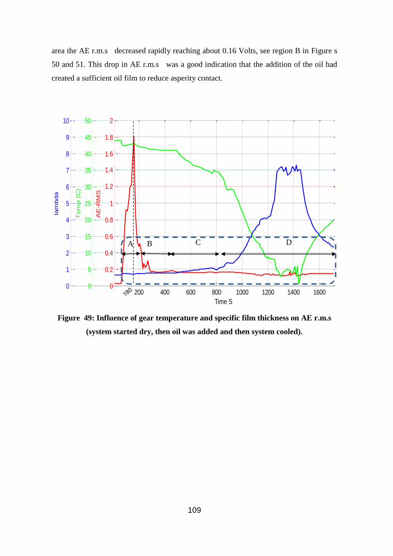
109
area the AE r.m.s decreased rapidly reaching about 0.16 Volts, see region B in Figure s
50 and 51. This drop in AE r.m.s was a good indication that the addition of the oil had
created a sufficient oil film to reduce asperity contact.
Figure 49: Influence of gear temperature and specific film thickness on AE r.m.s
(system started dry, then oil was added and then system cooled).
200 400 600 800 1000 1200 1400 16000
0.2
0.4
0.6
0.8
1
1.2
1.4
1.6
1.8
2
Time S
AE
-RM
S
0
5
10
15
20
25
30
35
40
45
50
Tem
p (
C)
0
1
2
3
4
5
6
7
8
9
10
lam
bda
A B D C

110
Figure 50: Gear temperature, specific film thickness and AE r.m.s as Figure 50
but enlarged
Figure 51: Influence of gear temperature and specific film thickness on AE
waveforms (the waveforms correspond to the regions in Figure 50)
200 400 600 800 1000 1200 1400 16000
0.1
0.2
0.3
0.4
0.5
Time S
AE
-RM
S
0
5
10
15
20
25
30
35
40
45
50
Tem
p (
C)
0
1
2
3
4
5
6
7
8
9
10la
mbda
0 0.01 0.02 0.03 0.04 0.05 0.06 0.07 0.08 0.09 0.1-0.4
-0.2
0
0.2
0.4
0 0.01 0.02 0.03 0.04 0.05 0.06 0.07 0.08 0.09 0.1-0.4
-0.2
0
0.2
0.4
0 0.01 0.02 0.03 0.04 0.05 0.06 0.07 0.08 0.09 0.1-0.4
-0.2
0
0.2
0.4
Am
plit
ude(v
olt)
0 0.01 0.02 0.03 0.04 0.05 0.06 0.07 0.08 0.09 0.1-0.4
-0.2
0
0.2
0.4
Time(s)
D C B A
B - Touch teeth with oil (BL)
C - Before cooling stage (EHL)
D - Cooling stage (HL)
A - Before adding oil stage (dry)

111
Region B of Figure s 50 and 51 represents the time frame from the instant oil was added
to the gearbox to the point where the oil levels had reached a height such that the gear
wheel teeth was in continuous contact with the oil in the sump. Within region B, during
the initial stages fluctuating levels in AE r.m.s were noted. The calculated λ value was
less than 1, suggesting a boundary lubrication regime. In addition, observations of the
waveform characteristics associated with this region, see waveform B in Figure 52,
showed transient AE bursts at the start of the signal but continuous type characteristics
towards the end of the signal. Given that large transient bursts are directly associated with
asperity contact at the mesh, this observed characteristic would suggest a contact region
of varying levels of asperity contact during the shaft revolution, indicative of a boundary
type regime.
Region C in Figure s 50 and 51 is associated with the period when the gears continuously
dipped into the oil, i.e, there was now a sufficient lubrication supply. The AE r.m.s level
in this region was 0.158 Volts and specific film thickness exceeded unity, λ ≥1, so region
C in Figure 51 is where the elastohydrodynamic regime became dominant.
The same procedure was followed as for the previous test and very similar results were
observed; a decrease in AE r.m.s as specific film thickness increased, and vice-versa.
These results indicate that AE technology can detect and distinguish the difference in oil
film thickness and thereby the lubrication regimes (e.g. EHL or HL).
In conclusion the results of this study indicate that the direct contact between the helical
gear teeth in dry conditions was a significant source of AE energy, confirming that
asperity contact is an essential source of AE signals. The results also showed that level of
the AE signal could be used to identify the lubrication film regime. A reduction in
specific film thickness resulted in an increase in AE r.m.s level and increasing the
specific film thickness significantly reduced AE r.m.s level. The results indicate the
potential of AE technology to predict and quantify lubrication film regime under different
operating conditions for helical gears.
112
Applicability of AE in Monitoring Defects During Dry and Lubricated 6.4
Contact
6.4.1 Test Instrumentation and Procedure
The test setup was similar to that of the previous tests, i.e. the same back to back gearbox
shown in Figure s 28 and 29.The teeth were damaged naturally by running the gears for a
prolonged period. Eventually, spalls, 2 mm diameter and 2 mm in depth, were noted on
six teeth, see circulated at teeth in Figure 53.
This test explores the influence of oil film thickness on the generation of AE from a
defective helical gear. The test programme undertaken measured the AE energy
generated during the mesh of a defective helical gear whilst simultaneously varying the
thickness of the lubricating oil. The latter was accomplished by spraying the liquid
nitrogen onto the test gear whilst it was in operation. This reduced the temperature of the
metal of the gear which also reduced the lubricant temperature, thus increasing the
lubricant viscosity and specific film thickness. The arrangement allowed the in-situ
variation of the film thickness in a controlled manner.
Defective teeth
on tested pinion
Figure 52: Defective Teeth – spalls of 2 mm diameter and 2 mm depth

113
To chieve fully dry running conditions the oil present in the gearbox was removed and
then the gear teeth surfaces and gearbox housing were thoroughly cleaned with acetone,
this was the same procedure as previously.
Again the AE r.m.s , AE waveforms were measured and recorded and the oil viscosity
estimated at the measured pinion temperature, using the same approach as adopted in the
previous tests.
6.4.2 Observation of The Signals in Time and Frequency Domains
Figure 54 presents the r.m.s value of the AE signal obtained with dry, EHL and HL
lubrication regimes; regions ‘A’, ‘B’ and ‘C’ respectively. As explained previously under
dry conditions the gear load is carried by tooth surface asperities. The gears were run dry
for 200s before lubricating oil was added, see region ‘A’ in Figure 54. Figure 55 shows
samples of AE raw waveforms captured at intervals during the test. Waveform ‘A’ in
Figure 55 was associated with dry region, ‘A’ in Figure 54, and so on. Under dry
running conditions it can be seen that there were transient bursts in the AE signal which
were superimposed onto a continuous type emission. These were attributed to asperity
contacts of the defective gears (dashed circle in waveform ‘A’)
Figure 53: Influence of gear temperature and specific film thickness on AE r.m.s
200 400 600 800 1000 1200 1400 1600 1800 20000
0.1
0.2
0.3
0.4
0.5
Time S
AE
-RM
S(v
olts)
0
5
10
15
20
25
30
35
40
45
50
Tem
p (
C)
0
5
10
15
Specific
Oil F
ilm
Thic
kness(lam
bda)
Gears returned under (EHL)
Cooling stage, Gears
operating under (HL)
Normal Gears operating under (EHL)
C (EHL) D (HL) A (Dry) B (BL)

114
Region ‘B’ of Figure 54 is associated with the period when the gears continuously dip
into the oil (the gearbox operates under normal conditions). The AE r.m.s level had an
average value of 0.17 Volts, and specific film thickness was greater than unity, λ ≥1.
Region ‘B’ in Figure 54 is indicative of a regime where EHL dominates. Waveform B in
Figure 55 shows transient AE bursts which are noticeably smaller than those noted under
dry conditions (region A). This significant reduction was predictable and attributed to the
presence of an oil film in the meshing area, causing partial separation between
corresponding asperities of defects (dashed circle in waveform B) on gear teeth in the
contact area. Thus in the EHL regime the generation of AE amplitude is relatively lower
than under dry conditions.
Figure 54: AE waveforms associated with regions ‘A’, ‘B’, ‘C’ in Figure 54
0 0.01 0.02 0.03 0.04 0.05 0.06 0.07 0.08 0.09 0.1-0.5
0
0.5
Time(s)
0 0.01 0.02 0.03 0.04 0.05 0.06 0.07 0.08 0.09 0.1-0.5
0
0.5
0 0.01 0.02 0.03 0.04 0.05 0.06 0.07 0.08 0.09 0.1-0.5
0
0.5
0 0.01 0.02 0.03 0.04 0.05 0.06 0.07 0.08 0.09 0.1-0.5
0
0.5
Am
plitu
de(v
olt)
A (Dry)
C (EHL)
D (HL)
B (BL)

115
With the introduction of nitrogen into the operation at 1100 seconds there was a sharp
decrease in gear metal temperature and a rapid fall in AE r.m.s . The drop in AE level
was a direct result of increasing viscosity and oil film thickness at the meshing area. The
AE r.m.s reached its minimum, approximately 0.13 Volts when the specific film
thickness was at its maximum, λ= 14.
Waveform C in Figure 55 was captured in the minimum temperature region, where
specific film thickness was a maximum and corresponding by the AE waveform showed
the lowest amplitude. It was noted that transient bursts were hardly distinguishable from
the continuous emissions. This confirmed that increasing oil film thickness decreased the
AE generated from the defective gears. The increased film thickness under this region
prevented the asperities in the defective region from meeting with the mating gear. This
explains the lack of a transient AE burst associated with the defect in the captured
waveform, see Figure 55.
The nitrogen supply was stopped when the gear temperature reached 0˚C, at about 1420
s, see region C in Figure 54. The gearbox continued operating and the temperatures of
lubricant and metal gradually returned to their initial values, with a corresponding
increase in AE levels as the specific film thickness decreased with increase in
temperature. The AE signals associated with the presence of surface defects on the pinion
tooth face showed no change in frequency content.
Statistical parameters obtained from the AE raw wavefo r.m.s ; Kurtosis (KURT) and
crest factor (CF) were used to compare the effect of film thickness in measuring the
presence of a defect, see Figure 55. These parameters were chosen on the basis that they
are commonly used for condition monitoring of gears, and were used above, see Figure
56 because they were used above which demonstrated that both Kurtosis and Crest Factor
could be used to detect the the presence of a fault, depending on oil temperature.
It can be seen that the highest levels of Kurtosis and Crest Factor were noted under dry
conditions. The Kurtosis value rapidly decreased as the oil regime proceeded from dry to
EHL. A similar reduction was noted for the CF. Further increases in film thickness
resulted in further reductions of Kurtosis and CF values. These results were noted for all

116
experiments and reaffirm the finding that the level of film thickness greatly influences the
generation of AE associated with defective gears.
Figure 55: Statistical parameters associated with AE waveform for different
lubrication regimes.
0
5
10
15
20
25
30
0
5
10
15
20
25
0 1 2 3 4 5
CF
ku
rto
sis
(KU
R)
CF KUR
Dry contact
EHL regime
1<λ<10
HL regime
λ>10
Spicific Film Thickness (λ)

117
Spectral Kurtosis of AE Signal from Defective and Non-Defective Gear 6.5
The meshing of helical gears is progressive due to the gradual increase and decrease in
contact length over a particular tooth face. Background noise masks the signal of interest
and the Kurtosis obtained is low. When there is strong background noise the Spectral
Kurtosis (SK) has been used instead of the global Kurtosis. The SK is a technique that
calculates the Kurtosis locally in different frequency bands. SK has been used to identify
a filter to select the part of the signal that is most impulsive, considerably reducing the
background noise and improving the diagnostic capability and it is suggested that its
application is appropriate here (Antoni, 2006; Sawahli and Randall, 2004).
Figure s 52 and 55 show peaks contained within the wavefo r.m.s , but the peaks are
different in size and the time intervals between the peaks vary due to the helical gear’s
contact mechanism. In Figure 55 the interval exactly reflects passage of the wheel over
the cracked pinion teeth. The existence of peaks showed that the signal contained a
number of impulses, which should be detected using spectral kurtosis.
The use of SK would effectively de-noise the AE signals for both defect free and
defective gear tests. The process involved calculating the Kurtogram for each signal for
which the bandwidth and center frequency are required for the design of a band-pass
filter. The determination of the SK was based on the algorithm developed by (Antoni and
Randall, 2006; Antoni, 2007).
A Kurtogram of signals from defect free and defective gear tests are presented in Figure s
57and 58 respectively for each of the four lubrication regimes (dry, BL, EHL and HL).
The center frequency (Fc) , bandwidth and max kurtosis were presented in Table 7.

118
Figure 56: Kurtogram for defect free test; waveforms ‘A’ to ‘D’ correspond to regions
‘A’ to ‘D’ in Figure 50
frequency [Hz]
level
k
fb-kurt.2 - Kmax
=4.8 @ level 1.5, Bw= 833333.3333Hz, fc=416666.6667Hz
0 0.5 1 1.5 2 2.5
x 106
0
1
1.6
2
3
3.2
3.4
3.6
3.8
4
4.2
4.4
4.6
4.8
frequency [Hz]
level
k
fb-kurt.2 - Kmax
=3.3 @ level 1.5, Bw= 833333.3333Hz, fc=416666.6667Hz
0 0.5 1 1.5 2 2.5
x 106
0
1
1.6
2
1.8
2
2.2
2.4
2.6
2.8
3
3.2
frequency [Hz]
level
k
fb-kurt.2 - Kmax
=1.4 @ level 3, Bw= 312500Hz, fc=1093750Hz
0 0.5 1 1.5 2 2.5
x 106
0
1
1.6
2
2.6
3
0.2
0.4
0.6
0.8
1
1.2
1.4
frequency [Hz]
level
k
fb-kurt.2 - Kmax
=1.2 @ level 1.5, Bw= 833333.3333Hz, fc=416666.6667Hz
0 0.5 1 1.5 2 2.5
x 106
0
1
1.6
2
2.6
30.2
0.4
0.6
0.8
1
1.2
Region (B)
Region (A)
Region (C)
Region (D)

119
Figure 57: Kurtogram for defective gear test; waveforms ‘A’ to ‘D’ correspond to regions
‘A’ to ‘D’ in Figure 54
frequency [Hz]
level
k
fb-kurt.2 - Kmax
=28.1 @ level 3.5, Bw= 208333.3333Hz, fc=520833.3333Hz
0 0.5 1 1.5 2 2.5
x 106
0
1
1.6
2
2.6
3
3.6
4 5
10
15
20
25
frequency [Hz]
level
k
fb-kurt.2 - Kmax
=21.2 @ level 7.5, Bw= 13020.8333Hz, fc=397135.4167Hz
0 0.5 1 1.5 2 2.5
x 106
0
1
1.6
2
2.6
3
3.6
4
4.6
5
5.6
6
6.6
7
7.6
8
4
6
8
10
12
14
16
18
20
frequency [Hz]
level
k
fb-kurt.2 - Kmax
=3.1 @ level 8, Bw= 9765.625Hz, fc=317382.8125Hz
0 0.5 1 1.5 2 2.5
x 106
0
1
1.6
2
2.6
3
3.6
4
4.6
5
5.6
6
6.6
7
7.6
80
0.5
1
1.5
2
2.5
3
frequency [Hz]
leve
l k
fb-kurt.2 - Kmax
=1.6 @ level 1.5, Bw= 833333.3333Hz, fc=416666.6667Hz
0 0.5 1 1.5 2 2.5
x 106
0
1
1.6
2
2.6
3
3.6
4
4.6
5
0
0.5
1
1.5
Region (B)
Region (A)
Region (D)
Region (C)
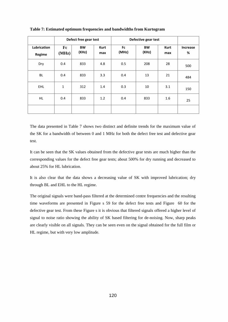
120
Table 7: Estimated optimum frequencies and bandwidths from Kurtogram
Defect free gear test Defective gear test
Lubrication
Regime
Fc
(MHz)
BW (KHz)
Kurt max
Fc (MHz)
BW (KHz)
Kurt max
Increase %
Dry 0.4 833 4.8 0.5 208 28 500
BL 0.4 833 3.3 0.4 13 21 484
EHL 1 312 1.4 0.3 10 3.1 150
HL 0.4 833 1.2 0.4 833 1.6 25
The data presented in Table 7 shows two distinct and definite trends for the maximum value of
the SK for a bandwidth of between 0 and 1 MHz for both the defect free test and defective gear
test.
It can be seen that the SK values obtained from the defective gear tests are much higher than the
corresponding values for the defect free gear tests; about 500% for dry running and decreased to
about 25% for HL lubrication.
It is also clear that the data shows a decreasing value of SK with improved lubrication; dry
through BL and EHL to the HL regime.
The original signals were band-pass filtered at the determined centre frequencies and the resulting
time waveforms are presented in Figure s 59 for the defect free tests and Figure 60 for the
defective gear test. From these Figure s it is obvious that filtered signals offered a higher level of
signal to noise ratio showing the ability of SK based filtering for de-noising. Now, sharp peaks
are clearly visible on all signals. They can be seen even on the signal obtained for the full film or
HL regime, but with very low amplitude.

121
Figure 58: AE waveforms associated with filtered signals (defect free test)
0 0.005 0.01 0.015 0.02 0.025-0.4
-0.3
-0.2
-0.1
0
0.1
0.2
0.3
0.4
Time(s)
Am
plitu
de(v
olts
)
0 0.005 0.01 0.015 0.02 0.025-0.3
-0.2
-0.1
0
0.1
0.2
Time(s)
Am
plitu
de (
volts)
0 0.005 0.01 0.015 0.02 0.025-0.1
-0.08
-0.06
-0.04
-0.02
0
0.02
0.04
0.06
0.08
0.1
Time(s)
Am
plitu
de(v
olts)
0 0.005 0.01 0.015 0.02 0.025-0.1
-0.05
0
0.05
0.1
Time(s)
Am
plitu
de (
volts)
Region (B)
BL regime
Region (A)
Dry regime
Region (C)
EHL regime
Region (D)
BL regime
Original signals Filtered signals

122
Figure 59: AE waveforms associated with filtered signals (test with defective gear)
0 0.01 0.02 0.03 0.04 0.05 0.06 0.07 0.08 0.09 0.1-0.5
-0.4
-0.3
-0.2
-0.1
0
0.1
0.2
0.3
0.4
0.5
Time(s)
Am
plitu
de(v
olts
)
0 0.01 0.02 0.03 0.04 0.05 0.06 0.07 0.08 0.09 0.1-0.4
-0.3
-0.2
-0.1
0
0.1
0.2
0.3
0.4
Time(s)
Amlpl
itude
(volt
)
0 0.01 0.02 0.03 0.04 0.05 0.06 0.07 0.08 0.09 0.1-0.15
-0.1
-0.05
0
0.05
0.1
0.15
0.2
Time(s)
Ampli
tude
(volt
s)
0 0.01 0.02 0.03 0.04 0.05 0.06 0.07 0.08 0.09 0.1-0.2
-0.15
-0.1
-0.05
0
0.05
0.1
0.15
Time(s)
Am
plitu
de(v
olts
)
Region (B)
BL regime
Region (A)
Dry regime
Region (C)
EHL regime
Region (D)
BL regime
Original signals Filtered signals

123
Kurtosis (KURT) and Crest Factor (CF) are traditional methods to measure the smoothness of a
signal and any increase in the spikiness of the signal profile will result in an increase in K and CF
values. Both K and CF are used to detect the onset of machine failure, and have also been
effective in monitoring the development of cracks and spall (Naid et al., 2009) (Tandon and
Choudhury, 1999; Vecer et al., 2005). Here the relative abilities of K and CF to detect a gear fault
have been compared before and after filtering.
The K values of the AE signals for the four lubrication regimes with no seeded fault (shown as
regions A to D in Figure 51) prior to, and after, filtering are presented in Figure 61. It can be
seen that the K value for the AE signal measured for the dry regime increased from 4.8 to 13 on
filtering, and the increase for full film lubrication was 1 to 1.6. In every case the filtered K value
was at least three times that obtained for the unfiltered signal, as can be seen from Figure 60, the
presence of spikes was much more evident with the filtered wavefo r.m.s .
There was also an increase in the CF value on filtering the AE signal. This was not as dramatic as
for the K values but still significant. In each lubrication regime the CF after filtering was at least
10% greater than for the unfiltered signal.
As expected the values of both K and CF decreased as the lubrication improved, and this is
explained as due to the effect of the lubricating regime on the spikiness of the AE signal.
Figure 62 shows the K and CF values for AE signals from the defective gear test. For the dry
regime the increase in CF levels rose from about 12.5 to about 14 on filtering and for full
lubrication doubled from 8 to 16 on filtering the raw signal. However, K levels rose from 28 to
200 for the dry regime and levels rose from 1 to 2 at HL regime.

124
Figure 60: Effect of band pass filtering of raw AE signal on KURT and CF (Defect free
gear test)
0
2
4
6
8
10
12
14
Dry BL EHL HL
KURT for Unfiltered Signal
KURT for filtered Signal basedSK
0
2
4
6
8
10
12
14
16
Dry BL EHL HL
CF for Unfiltered signal
CF for filtered signal based SK

125
Figure 61: Effect of band pass filtering of raw AE signal on KURT and CF (defective gear
test)
0
50
100
150
200
250
Dry BL EHL HL
KURT for Unfiltered Signal
KURT for filtered Signal based SK
0
5
10
15
20
25
30
35
Dry BL EHL HL
CF for Unfiltered signal
CF for filtered signal based SK

126
Correlation of AE r.m.s With Specific Film Thickness (λ) 6.6
Results showed the relationship between AE r.m.s and the calculated specific film
thickness (λ) for both defect free and seeded defect tests. The test gears experienced three
lubrication regimes from dry lubrication regime with λ =0 through BL, EHL and HL
regimes. It was noted that the highest levels of AE r.m.s were in dry region, about 0.5
volts in the non-defective tests and 1 volt with seeded defects. There was a decrease in
AE levels with the addition of lubricating oil; from direct (dry) contact to the BL region
where the teeth were still in partial direct contact with λ about unity. It was clearly
observed that the AE r.m.s levels were higher (0.20 volts) when the seeded defects were
present than for the defect free test (0.16 volts).
The AE r.m.s levels decreased with increased thickness of lubricant film. It is believed
that AE sources in this region come from either asperity contact and/or the elastic
deformation of the teeth at contact. Again was clear that AE r.m.s levels obtained for
seeded defects were higher. If asperity contact is the main contributor to AE activity, then
when the specific film thickness increased to a value of λ = 9 when asperity contact
would be expected to disappeared, there should be no further reduction in AE levels with
increased lubrication.

127
General Observations 6.7
Significant events noticed and observed during the tests which will be important
when analysing the AE signal in later sections are:
At the point where liquid nitrogen was initially introduced onto the wheel (t =500
seconds), see Figure 48, there was a slight increase in AE activity which increased
significantly when the temperature of the gear fell to below 35oC. See regions ‘A’ and
‘B’ in Figure 48, and in particular the trace included within the dotted circle. This
peak in AE r.m.s level lasted from about 500 to 650 seconds and occurred even
though there was a continuous increase in specific film thickness (λ) during this time.
This was attributed to the micro-structural change in the gear material as the
temperature of the gear was reduced rapidly. This micro-structural change contributed
to the generation of AE activity and thus increased the AE r.m.s level. After this
micro-structural change was stabilised, the continuous increase in specific film
thickness (λ) reduced the AE r.m.s level.
During the actual tests, the effect of these macro- and micro-structural changes in
gear metal due to the rapid change in temperature (from approximately 50ºC+/- to
0ºC) in a very short period of time (typically less than 10 minutes) caused extraneous
AE activities. These extraneous AE activities contributed to the higher AE r.m.s .
Also it was observed that the AE r.m.s started to decrease rapidly when temperature
reached about 15°C.
During the experiment, the oil mist generated as a result of churning of the oil formed
a “frozen mist” as the oil temperature approached 0°C. This frozen oil mist was
thrown into the gear mesh by the rotating wheel resulting in the generation of AE
activity. This sudden increase in activity is shown in Figure 48 in the dotted circle in
region ‘C’. It was not possible to control the entry of the frozen mist into the gear
mesh.
The region between A and B (dotted circle) shown in Figure 51 also a sudden
increase in AE r.m.s level as drops of oil were first dripped onto the gear wheel (at
about 240s). It is suggested that adding oil in this manner and quantity results in oil
drag and oil friction. This effect lasted for about 60s.

128
Chapter 7
Conclusions and
Future Work

129
7 Conclusions and Future Work
Conclusions 7.1
An AE sensor was used to monitoring oil film thickness at contact area between the gear
teeth in real-time for vary oil temperature conditions. At constant speed and load the
operating temperature plays a role in surface fatigue and micropitting. As the temperature
at the contact area increases, the oil viscosity is reduced and film thickness decreases.
Thus a lubricant with too low an initial viscosity will become too thin and not provide
adequate protection as the gear temperature increases leading to an increased rate of
micropitting and surface fatigue.
A thorough analysis of oil film regime detection in helical gears has been presented. This
analysis included a review of online condition monitoring methodologies for gears. In
this research programme tests have been conducted, on a back-to-back gearbox,
investigating the effects of changes in lubrication and gear temperatures at constant load
and speed.
This research has investigated the application of acoustic emission to the identification of
oil film regime in helical gear and used advanced signal processing techniques to analyse
the AE signals, and several conclusions have been drawn based on the results and
observations.
Firstly, mechanisms and factors that influence the generation of AE activities during
helical gear mesh have been identified. The project has compared AE and vibration
signals from the gears for condition monitoring and diagnosis of defect free and seeded
surface defect on the gears in the presence of temperature variations. The AE signal
showed better sensitivity for early diagnosis of the seeded damage compared to
vibration. The AE signal showed a high sensitivity to identifying the presence of gear
surface faults and was capable of detecting incipient damage in helical gears, far better
than the vibration signals. Because pitch point contact for helical gear mesh is
progressive pure rolling activities occur during meshing, resulting in the series of
transient bursts that are so closely spaced as to form high amplitude continuous types of
wavefo r.m.s .

130
Results presented here (Section 1.1) show that for constant speed and load, increasing the
oil temperature in the gear system or introducing a tooth fault had negligible effect on
vibration r.m.s as measured at both the bearing pedestal and gearbox case. The AE
measurements for the sensor placed on the gearbox casing also showed no significant
change with change in oil temperature or seeded defect. However, for the AE sensor on
the gear the presence of the seeded fault had considerable effect on Kurtosis and Crest
Factor of the AE signal when the temperature of the lubricating oil reached 36oC.
The influence of calculated lubrication specific film thickness (λ) on AE generation was
experimentally investigated and reported (Section 6.2). The change in specific film
thickness, as calculated from the gear metal temperature, suggests that λ has a substantial
effect on AE generation. The results obtained show an inverse relationship between
specific film thickness λ and AE r.m.s level, strengthening the view that asperity
contact is the main source of AE during helical gear meshing. The results confirm the
potential of AE technology to predict and quantify lubrication film regime and suggests
that the AE signal can be used for assessing the level of asperity contact under a variety
of temperatures in real time operation. Because the level of asperity contact is influenced
by the lubricant film thickness and surface roughness, AE technique can be a useful tool
in detecting lubricating film breakdown and/or degradation of contact surfaces.
The investigation showed that in dry conditions (Section 6.3) a significant source of AE
energy was direct contact between the helical gear teeth and the level of the AE signal
demonstrated that this was a method that would readily detect dry gear running, further
confirming that asperity contact is an important source of the AE signals. If accurately
monitored the detection AE offers of running dry would, in practice, severely reduce the
occurrence of gearbox destruction.
The rapid decline in the AE levels, resulting from introducing even a small amount of
lubricating oil directly onto the gear provides evidence of the potential of AE technology
to predict the transition from dry regime to the boundary regime BL. Its high sensitivity
can provide an early warning of instability and it does not require measurements to be
taken over a prolonged period to establish that gear distortions are occurring. In addition,
it can provide a real-time indication of oil regime-dependent stability. Acoustic emission

131
technology has the potential to provide an effective lubrication regime monitoring
system. The AE signal was lowest at the highest values of the specific film thickness and
this is evidence to transition from the EHL to the HL regime. The results also showed
that under lubricating conditions that completely separate the gear surface asperities, the
generation of AE due to the presence of a defect may not be detectable over typical
background noise.
Diagnosis of detective gear during dry and lubricated contact, which naturally degraded,
has been investigated (Section 6.4) and the results provided the ability to identify gear
defects under different lubricating regimes has been explored. It has been demonstrated
that under lubricating conditions that completely separate the gear surface asperities, the
generation of AE due to the presence of a defect may not be detectable over typical
background noise level.
Spectral Kurtosis and Kurtograms were investigated as analysis tools for the AE signal
for monitoring non-defective and naturally defective gears (Section 6.5). It was shown
that the application these techniques was effective in de-noising the AE signals. The
Kurtogram identified a frequency band in which the measure of the spikiness of the
signal profile was greatest. Of the statistical parameters considered, variation of kurtosis
values for the filtered raw AE data provides basis for a better understanding for lubricant
film deterioration and fault progression.
Future Work 7.2
This research has made a contribution to knowledge; it has demonstrated that AE is a
powerful diagnostic tool for identifying gear lubrication film regime and for early
diagnosis of gear faults. This research has also opened new doors for the exploration of
using AE signal analysis that could form the foundation for a significant advance in the
application of AE for the prediction of the remaining life time of gears. The author hopes
that the work presented in this thesis will stir the thoughts and generate new ideas in
readers that will contribute to the advancement of gear engineering and the technologies
used for detecting and diagnosing oil film thickness in geared transmission systems.

132
The findings of this research are encouraging and promising for the development of AE
technology as preventative maintenance approach for early fault detection and prevention
in all types of gearboxes. However further research is needed in critical areas.
Recommendations for future work include:
The signal from the gearbox casing typically experiences a high level of attenuation
and it is expected, lower a SNR, making defect identification more challenging. In the
future work the sensors on the casing might be mounted using such techniques as
waveguides, and more advanced time/frequency analysis methods.
Investigate the combined influence of wear, lubrication and contact mechanics on AE
generation in helical gears. This could be realised by undertaking tests on specially
designed machines such as a wear or tribology machine.
Finding new technique for controlling and measuring the temperature inside the gear
mesh would be very beneficial in obtaining a close approximation for the specific
film thickness (λ) during gear operations. The use of liquid nitrogen during the tests
was problematic particularly because of the formation of thick very low temperature
lubricant mists at entered the gear mesh and generated unwanted AE signals. Varying
the specific film thickness (λ) using other techniques would overcome this problem.
Further work is needed to investigate the wear development of helical gears and
correlate specific oil film thickness λ, asperity contact and wear rate.

133
hapter 8
References

134
8 References
Alexander, D. (1992), "The viscosity of lubricants", Lubrication, vol. 78, no. 3, pp. 1-16.
AlKazzaz, S., Ahmed, S. and Singh, G. (2003), " Experimental investigations on induction
machine condition monitoring and fault diagnosis using digital signal processing
techniques", Electric Power Systems Research, vol. 65, pp. 197-221.
Antoni, J. (2004), "The Spectral Kurtosis of non-stationary signals some properties and
applications ", Proc Eurasip, , pp. 1167-1170.
Antoni, J. (2006), "The spectral kurtosis: A useful tool for characterising non-stationary
signals", Mechanical Systems and Signal Processing, vol. 20, pp. 282-307.
Antoni, J. (2007), "Fast computation of the kurtogram for the detection of transient faults",
Mechanical Systems and Signal Processing, vol. 21, pp. 108-124.
Antoni, J. and Randall, R. B. (2006), " The spectral kurtosis: Application to the vibratory
surveillance and diagnostics of rotating machines", Mechanical Systems and Signal
Processing, vol. 20, pp. 308-331.
Ashley, M. (2008), Mixing Lubricants: A Recipe For Trouble, machinerylubrication, U.S.
ASM. (ed.) (1992), Friction, Lubrication and Wear Technology, ASM International; 10th
edition.
B. O. H, L. (2011), null, Aircraft Accident Report No: 2/2011, AAIB Bulletin, UK.
Balderston, H. L. (1969), "The detection of incipient failure in bearings", materials
rvaluation, vol. 27, no. 6, pp. 121-128.
Bankim and Bernard, J. H. (1882), Frictional Heating Due to Asperity Interaction of
Elastohydrodynamic Line-Contact Surfaces (unpublished Technical Paper), NASA.
Beattie, A. and Rumsey, M. (1999), "Non-Destructive Evaluation of Wind Turbine Blades
Using an Infrared Camera", ASME Wind Energy Symposium,18th, Aerospace Sciences
Meeting and Exhibit, 37th, Vol. 18th, Reno, Nevada.

135
Becker, W. T. and Shipley, R. J. (eds.) (2002), Failure Analysis and Prevention (ASM
HandbookVolume 11), 10th ed, ASM, US.
Benabdallah, H. and Aguilar, D. (2008), "Acoustic emission and its relationship with friction
and wear for sliding contact", Tribology Transactions, vol. 51, no. 6, pp. 738-747.
Benbouzid, M. E. H. (2000), "A review of induction motors signature analysis as a medium
for faults detection", IEEE Transactions on Industrial Electronics, vol. 47, no. 5, pp. 984-
993.
Board, D. B. (1975), "Incipient failure detection in high speed machinery", Vol. 10th
Symposium, 23-25 April, San Antonio, .
Boczar, T. and Lorenc, M. (2004), "Determining the Repeatability of Acoustic Emission
Generated by the Hsu-Nielsen Calibrating Source", Molecular and Quantum Acoustics,
vol. 25, no. ., pp. 177-191.
Boness, R. and McBride, S. (1991), "Adhesive and abrasive wear studies using acoustic
emission techniques", Wear, vol. 149, no. 1, pp. 41-53.
Boness, R., McBride, S. and Sobczyk, M. (1990), "Wear studies using acoustic emission
techniques", Tribology International, vol. 23, no. 5, pp. 291-295.
Boyer, E. B. (1975), Failure Analysis and Prevention , Metal Handbook ed, Ohia, American
Society for Metals., U.
Brüel and Kjaer. (1981), "(1981) Technical Review", vol. ISSN:0007- 2621, no. 2, pp. 38-
40.
BS EN (2009), BS EN 1330-9:2009 Non-destructive testing— Terminology, , BS, UK.
BS EN 13477-1:2001. (2001), Non-destructive testing - Acoustic emission - Equipment
characterization, Part 1, BS, UK.
Cairns, M. (1991), The Condition Monitoring of a Spur gearbox Using Noise and Vibration
Measurements and Correlation (unpublished MSc thesis), Cranfield University, UK.

136
Capgo Pty Ltd. (2009), Fatigue Detection by Acoustic Emissions, Capgo Pty Ltd, available
at: http://www.capgo.com/Resources/ConditionMonitoring/Acoustic.html (accessed
12/2012).
Choy, F. K. S., Huang, J. J. and Zakrajsek, R. F. (1994), Vibration signature analysis of a
faulted gear transmission system, 106623. AIAA-94-2937, University of Akron,
University of Akron.
ClickGreen, s. (2012), Offshore wind will play a vital role in the UK's future energy mix,
report confi r.m.s , , ClickGreen, UK.
Copper, P. (1983), "Wear debris monitoring of rolling bearings", British Journal of NDT,
vol. 25, no. 2, pp. 75-83.
Czichos, H. (1977), "Influence of asperity contact conditions on the failure of sliding
elastohydrodynamic contacts", Wear, vol. 41, no. 1, pp. 1-14.
Da Silva, A. (1997), "Rotating machinery monitoring and diagnosis using short-time Fourier
transform and wavelet techniques", Knoxville, T. (ed.), in: Proc. Int. Conf. Maintenance
and Reliability, Vol. 1, pp. 14.01–14.15.
de Kraker, A. and Stakenborg, M. J. L. (1986), "Cepstrum analysis as a useful supplement to
spectrum analysis for gear-box monitoring ", stress analysis: proceedings of the 8th
international conference, Amsterdam, Netherlands, , May 12-16, Amsterdam,
Netherlands, pp. 181-190.
Dempsey, P., Lewicki, D. and Decker, H. (2004), Investigation of Gear and Bearing Fatigue
Damage Using Debris Particle Distributions.
, 2004-212883, NASA/TM.
Dowson, D. (1977), Elasto-hydrodynamic lubrication, 2nd ed, Pergamon, Oxford.
Dowson, D. (1995), "Elastohydrodynamic and micro-elastohydrodynamic lubrication",
Wear, vol. 190, no. 2, pp. 125-138.

137
Dowson, D. and Ehret, P. (1999), "Past, present and future studies in elastohydrodynamics",
Proceedings of the Institution of Mechanical Engineers, Part J: Journal of Engineering
Tribology, vol. 213, no. 5, pp. 317-333.
Drago, T. (ed.) (1988.), Fundamentals of gear design, Butterworths ed, Boston, London.
Drouillard, T. F. (ed.) (1988), Introduction to acoustic emission, Material Evaluation ed, 46,
174-179.
Dwyer Joyce, R. S. (1995), Tribological Design Data, , Institution of Mechanical Engineers
1995, UK.
Dwyer, R. (1983), " Detection of non-Gaussian signals by frequency domain Kurtosis
estimation", Acoustics, Speech, and Signal Processing, IEEE International Conference on
ICASSP, Vol. 8, pp. 607-610.
Dwyer-Joyce, R. S. (ed.) (1995), Lubrication, 1st ed, Tribological Design Data Part 2.
E. Richard Booser, P. D. (1983), CRC HANDBOOK of LUBRICATION (Theory and
Practice of Tribology)Volume IITheory & Design
, Volume II ed, Library of Congress, US.
Ebersbach, S., Peng, Z. and Kessissoglou, N. J. (2006), "The investigation of the condition
and faults of a spur gearbox using vibration and wear debris analysis techniques", Wear,
vol. 260, no. 1–2, pp. 16-24.
Eftekharnejad, B. and Mba, D. (2008), "Acoustic emission signals associated with damaged
helical gears", Insight: Non-Destructive Testing and Condition Monitoring, vol. 50, no. 8,
pp. 450-453.
Eftekharnejad, B. and Mba, D. (2009), "Seeded fault detection on helical gears with acoustic
emission", Applied Acoustics, vol. 70, no. 4, pp. 547-555.
Envirocoustics S. A. (2007), Acoustic Emission Theory, Envirocoustics S. A.Publications,
available at: http://www.envirocoustics.gr/acoustic_emission_theory_eng.htm (accessed
12/2012).

138
Eric Y, K., Andy, C. T., Bo-Suk, Y. and Vladis, K. (2007), "Experimental Study on
Condition Monitoring of Low Speed Bearings : Time Domain Analysis", Fifth
Australasian Congress on Applied Mechanics (ACAM 2007), Vol. 5th Australasian
Congress on Applied Mechanics, 10–12 December, Brisbane, Australia, ACAM, .
Evans, J. S. and Hunt, T. M. (eds.) (2008), Machine & systems condition monitoring series–
The oil analysis handbook, Firset ed, Coxmoor Publishing Company, Oxford, UK.
Faulstich, S. (2008), Windenergie Report Deutschland 2008, , Institut für Solare
Energieversorgungstechnik (Hrsg.), Kassel.
Fernandes, P. and McDuling, C. (1997), "Surface contact fatigue failures in gears",
Engineering Failure Analysis, vol. 4, no. 2, pp. 99-107.
Forrester, D. (1996), Advanced vibration analysis techniques for fault detection and
diagnostic in geared transmission systems (PhD thesis), Swinburne University of
Technology, Melbourne.
GABERSON, H. (2002), "The Use of Wavelets for Analyzing Transient Machinery
Vibration", S.V.Sound and Vibration, vol. 36, pp. 12-17.
Gitin M, M. (ed.) (1994), Handbook of Gear Design, Second Edition ed, Tata McGraw-Hill,,
©1989, New Delhi, India ; Montréal.
Guangteng, G., Cann, P. M., Olver, A. V. and Spikes, H. A. (2000), "An experimental study
of film thickness between rough surfaces in EHD contacts", Tribology International, vol.
33, no. 3–4, pp. 183-189.
Halme, J. and Andersson, P. (2010), "Rolling contact fatigue and wear fundamentals for
rolling bearing diagnostics – state of the art", Proceedings of the Institution of
Mechanical Engineers, Part J: Journal of Engineering Tribology, vol. 224, pp. 4.
Ham, C. W., Crank, E. J. and Rogers, W. L. (eds.) (1958), Mechanics of Machinery,
McGraw-Hill.
Hamrock J, B., Steven, R. S. and Jacobson, B. O. (eds.) (2004), Fundamentals of Fluid Film
Lubrication, Second ed, McGraw-Hill.
139
Hamzah, R. I., Al-Balushi, K. R. and Mba, D. (2008), "Observations of acoustic emission
under conditions of varying specific film thickness for meshing spur and helical gears",
Journal of tribology, vol. 130, no. 2.
Hamzah, R. I. and Mba, D. (2007), "Acoustic emission and specific film thickness for
operating spur gears", Journal of tribology, vol. 129, no. 4, pp. 860-867.
Hamzah, R. I. and Mba, D. (2009), "The influence of operating condition on acoustic
emission (AE) generation during meshing of helical and spur gear", Tribology
International, vol. 42, no. 1, pp. 3-14.
Handbook of metric gears (ed.) Handbook of metric gears - Product guide and technical
data: Catalog Q 410, .
Hasan, (2006), Gearbox Health Monitoring and Fault Detection Using Vibration Analysis
(PhD thesis), Dokuz Eylül University, Dokuz Eylül.
Henning, D. (1988), "Josef Kaiser: His achievement in acoustic emission research
", Material Evaluation, vol. 46, no. 2, pp. 193-195.
Höhn, B. and Michaelis, K. (2004), "Influence of oil temperature on gear failures",
Tribology International, vol. 37, no. 2, pp. 103-109.
Holroyd, T. (2000), Acoustic Emission & Ultrasonic, 1st ed, Coxmoor Publishing
Company's. Oxford, UK.
Holroyd, T. and Randall, N. (1993), "Use of acoustic emission for machine condition
monitoring", British journal of non-destructive testing, vol. 35, no. 2, pp. 75-78.
J, Y. and Quin˜o´nez, P. D. (2004), "Gear surface temperature monitoring", vol. IMechE
Vol. 219 Part J: J. Engineering Tribology, pp. 99-105.
Jardine, A. K., Lin, D. and Banjevic, D. (2005), A review on machinery diagnostics and
prognostics implementing condition-based maintenance, Technical report, CBM Lab,
Department ofMechanical and Industrial Engineering, University of Toronto.

140
Jardine, A. K. S., Lin, D. and Banjevic, D. (2006), "A review on machinery diagnostics and
prognostics implementing condition-based maintenance", Mechanical Systems and Signal
Processing, vol. 20, no. 7, pp. 1483-1510.
Jiaa, C. L. and Dornfeld, D. A. (1990), "Experimental studies of sliding friction and wear via
acoustic emission signal analysis", Wear, vol. 139, no. 2, pp. 403-424.
Jie, Z. and Drinkwater, B. W. (2006), "Acoustic measurement of lubricant-film thickness
distribution in ball bearings", J. Acoust. Soc. Am., vol. 119, no. 2, pp. 863-871.
Johnson, M. L. (2012), Lubrication Technology , available at:
http://www.sumitomodrive.com (accessed 06/05).
Joseph, R. D. (ed.) (2005), Gear materials, properties, and manufacture, Second Edition ed,
ASM International, 2005.
Kaiser, J. (1950), A study of acoustic phenomena in tensile tests, Dr.-Ing. Dissertation,
TechnicalUniversity of, Munich.
Kar, C. and Mohanty, A. R. (2006), "Multistage gearbox condition monitoring using motor
current signature analysis and Kolmogorov–Smirnov test", Journal of Sound and
Vibration, vol. 290, no. 1–2, pp. 337-368.
Keith, M. R. (2002), An introduction to predictive maintenance , Second ed, Elsevier
Science, U.S.
Krantz, K. and Kahraman, A. (2004), "An Experimental Investigation of the Influence of
Lubricant Viscosity and Additives on Gear Wear", Tribology Trans, vol. 47, pp. 138-148.
Kutz, M. (ed.) (2006), Mechanical engineers' handbook, 3rd ed, Wiley, Hoboken, N.J.
Le Sueur, H. E., (1978), Airworthiness of Hlicopters, 82(814), Aeronaut J, 82(814).
Lebold, M., McClintic, K. and Campbell, R. (2000), Review of vibration analysis methods
for gearbox diagnostics and prognostics, 634, ed. pp. 623, Proceedings of the 54th
Meeting of the Society for Machinery Failure Prevention Technology, Virginia Beach.

141
Lingard, S. and Ng, K. K. (1989), "An investigation of acoustic emission in sliding friction
and wear of metals", Wear, vol. 130, no. 2, pp. 367-379.
Liu, H., Lin, J. and Liangsheng, Q. (1997), "FFT Spectral Entropy and its application in fault
diagnosis", China Mech. Eng., vol. 4, no. E6.10, pp. 157-159.
Loutas, T. H. and Kalaitzoglou, J. (2007), "T.H. On the application of non-destructive
testing techniques on rotating machinery", 4th International Conference on NDT, 11-
14october, Chiania, Crete-Greece, NDT, .
Lucente, M. (2008), Condition monitoring system in wind turbine gearbox (MSc thesis),
KTH, Stockholm, Sweden.
Luke, D., ( 2012), Changing a Gear: Gearbox Lubrication and Its Impact on Wind Turbine
Lifespan, Wind Technology, Distributed with Renewable Energy World Magazine, UK.
Macconochie, I. O. and Newman, W. H. (1961), "The effect of lubricant viscosity on the
lubrication of gear teeth", Wear, vol. 4, no. Issue 1, pp. 10-21.
Manufacturing Association American Gear (ed.) (1989), Geometry Factors for Determining
the Pitting Resistance and BendingStrength of Spur, Helical, and Herringbone Gear
Teeth, 1st ed, Manufacturing Association American Gear, US.
Martin, K. F. (1978), "A Review of friction prediction in gear teeth", Wear, vol. 49, pp. 201-
238.
Mathew, J. (1989), Monitoring the vibration of rotating machine elements , 1, An overview.
The Bulletin of the Center of Machine Condition Monitoring, Monash University.
Matthew G, B., Dr Rhys, P. and Dr Karen M, H. (2004), Detection of fatigue crack growth
in aircraft landing gear, DGZfP-Proceedings BB 90, CD Lecture 27 EWGAE.
Mba, D. (2003), "Acoustic Emissions and Monitoring Bearing Health", STLE Tribol. Trans.,
vol. 46, no. 3, pp. 447-451.
Mba, D. and Rao, R. B. (2006), "Development of acoustic emission technology for condition
monitoring and diagnosis of rotating machines; bearings, pumps, gearboxes, engines and
rotating structures", Shock and Vibration Digest, vol. 38, no. 1, pp. 3-16.

142
McFadden, P. D. (1986), "DETECTING FATIGUE CRACKS IN GEARS BY
AMPLITUDE AND PHASE DEMODULATION OF THE MESHING VIBRATION",
Journal of Vibration, Acoustics, Stress, and Reliability in Design, vol. 108, no. 2, pp.
165-170.
McNiff, B. P. (1991), Variations in gear fatigue life for different wind turbine braking
strategies, SERI/TP-257-3984; CONF-9009107--7, DOE; USDOE, Washington, DC
(USA), United States.
Mechefske, C., G, S. and J, S. (2002), "Using Acoustic Emission to Monitor Sliding Wear",
INSIGHT - The Journal of the British Society of Non-Destructive Testing, vol. 44, no. 8,
pp. 490-497.
Miller, R. and McIntire, P. (eds.) (1987a), Acoustic emission testing. Nondestructive
, Second ed, Nondestructive testing handbook, American Society for Nondestructive
Testing.
Miller, R. K. and McIntire, P. (eds.) (1987b), Nondestructive testing handbook, volume 5:
Acoustic emission testing, 2nd ed, ASNT.
Mirhadizadeh, S. A. and Mba, D. (2009), "Observations of acoustic emission in a
hydrodynamic bearing", Journal of quality in maintenance engineering, vol. 15, no. 2, pp.
193-201.
Muller, J. and Errichello, R. L. (2001), How to analyze gear failures, January, Geartech.
Naid, A., Gu, F., Shao, Y. and Ball, A. (2009), "Bispectrum analysis of motor current
signals for fault diagnosis of reciprocating compressors", Key Engineering Materials, vol.
413 - 414, pp. 505-511.
NDT, E. R. C. (2013), Introduction to Acoustic Emission Testing, available at:
http://www.ndted.org/EducationResources/CommunityCollege/Other%20Methods/AE/A
E_Intro.htm (accessed 03/03).
Neale, M. J. (ed.) (1995), Tribology, 2nd ed, Butterworth-Heinemann, Oxford, UK.
143
Olver, A. V. (2002), "Gear lubrication - A review Part J. Journal of Engineering Tribology",
vol. 216, pp. 255-267.
Paula. J, D. (2001), Gear Damage Detection Using Oil Debris Analysis, NASA / TM--2001-
210936, NASA, Manchester, United Kingdom, September 4--6, 2001.
Pekka, V. (2006), Oil analysis in machine diagnostics, ISBN 951-42-8076-8, Acta
Universitatis Ouluensis A, University of Oulu.
Peng, Z., Kessissoglou, N. J. and and Cox, M. (2005), "A Study of the Effect of
Contaminant Particles in Lubricants using Wear Debris and Vibration Condition
Monitoring Techniques", Wear, vol. 258, no. 11-12, pp. 1651-1662.
Peter Lynwander (1983), Gear Drive Systems: Design and Application, Volume 20 of
Dekker Mechanical Engineering Series ed, Marcel Dekker.
Physical Acoustic Co. (2007), PCI-2 BASED AE SYSTEM USER's MANUAL, .
Pirro, D. M. and Wessol, A. A. (eds.) (2001), Lubrication Fundamentals, Second Edition:
Revised and Expanded, Second Edition ed, CRC Press.
Reimche, W. and Südmersen, U. (2003), "Basics of Vibration Monitoring for Fault
Detection and Process Control, vol. 6, pp. 2-6. Rio de Janeiro, Brazil (2003).", Vol. 6,
Rio de Janeiro, Brazil, pp. 2-6.
Ribrant, J. and Bertling, L. (2007), "Survey of failures in wind power systems with focus on
Swedish wind power plants during 1997-2005", Power Engineering Society General
Meeting, 2007. IEEE, Vol. 22, 24-28 June 2007, Tampa, FL, pp. 1 - 8.
Robinson, J. C. (2001), " Detection and Severity Assessment of Faults in Gearboxes from
Stress Wave Capture and Analysis", Society for Machinery Failure Prevention
Technology (MFPT) 2001 Annual Conference, 2001.
Roylance, B. J. and Hunt, T. M. (eds.) (1999), Machine & condition monitoring series –
Wear debris analysis, 1st ed ed, Coxmoor Publishing Company, Oxford, UK.

144
Ruqiang, Y. (2007), Base Wavelet Selection Criteria for Non-stationary Vibration Analysis
in Bearing Health Diagnosis (PhD thesis), University of Massachusetts, Online PhD
Thesis.
Samuel, P. D. and Pines, D. J. (2005), "A review of vibration-based techniques for
helicopter transmission diagnostics", Sound and Vibration, vol. 282, pp. 475-508.
Sarychev, G. A. and Shchavelin, V. M. (1991), " Acoustic emission method for research and
control of friction pairs", Tribology International, vol. 24, no. 1, pp. 11.
Sawahli, N. and Randall, R. (2004), "The application of spectral kurtosis to bearing
diagnostics", Proc Acoustics (ed.), in: null, Noveember 2004, Australia, pp. 393.
Serrato, R., Maru, M. M. and Padovese, L. R. (2007), "Effect of lubricant viscosity grade on
mechanical vibration of roller bearings", Tribology International, vol. 40, no. 8, pp. 1270-
1275.
Shigley, J. E., Mischke, C. R. and Brown, T. H. (eds.) (2004), Standard handbook of
machine design electronic resource, 3rd ed ed, McGraw-Hill, New York.
Shiroishi, J., Li, Y., Liang, S., Kurfess, T. and Danyluk, S. (1997), "BEARING
CONDITION DIAGNOSTICS VIA VIBRATION AND ACOUSTIC EMISSION
MEASUREMENTS", Mechanical Systems and Signal Processing, vol. 11, no. 5, pp. 693-
705.
Smith, J. D. (1993), "A new diagnostic technique for asperity contact", Tribology
International, vol. 26, no. 1, pp. 25-27.
Spinato, F., Tavner, P. J., van Bussel, G. J. W. and Koutoulakos, E., (2009), "Reliability of
wind turbine subassemblies", vol. 3, no. 4, pp. 1-15.
Stokes, A. (ed.) (1992), Manual Gearbox Design, Butterworth-Heinemann Ltd.
Stribeck, R. (1902), " Die Wesentlichen Eigenschaften der Gieit- und Rollenlager--the key
qualities of sliding and roller bearings. Zeitschrift des Vereines Seutscher Ingenieure",
vol. 46, no. 38, pp. 1342-1348.

145
Tan, C. K. (2005), An Investigation on the Diagnostic and Prognostic Capabilities of
Acoustic Emission on Spur Gearbox (PhD thesis), Cranfield University, UK.
Tan, C. K. and Mba, D. (2005), " Limitation of Acoustic Emission for Identifying Seeded
Defects in Gearboxes", Nondestructive Evaluation, vol. 24, no. 1, pp. 11-28.
Tan, C. K., Irving, P. and Mba, D. (2007), "A comparative experimental study on the
diagnostic and prognostic capabilities of acoustics emission, vibration and spectrometric
oil analysis for spur gears", Mechanical systems and signal processing, vol. 21, no. 1, pp.
208-233.
Tan, C. K. and Mba, D. (2005a), "Experimentally established correlation between acoustic
emission activity, load, speed, and asperity contact of spur gears under partial
elastohydrodynamic lubrication", Proceedings of the Institution of Mechanical Engineers,
Part J: Journal of Engineering Tribology, vol. 219, no. 6, pp. 401-409.
Tan, C. K. and Mba, D. (2005b), "Identification of the acoustic emission source during a
comparative study on diagnosis of a spur gearbox", Tribology International, vol. 38, no.
5, pp. 469-480.
Tandon, N. and Choudhury, A. (1999), "A Review of Vibration and Acoustic Measurement
Methods for the Detection of Damages in Rolling Element Bearings", vol. Tribology
International, 32(8), no. 1999, pp. 469–480.
Tekeo, Y. and Takashi, F. (1982), "A new acoustic emission source locating system for the
study of rolling contact fatigue", Wear, vol. 81, pp. 183-186.
Toutountzakis, T. and Mba, D. (2003), "Observations of acoustic emission activity during
gear defect diagnosis", NDT & E International, vol. 36, no. 7, pp. 471-477.
Toutountzakis, T., Tan, C. K. and Mba, D. (2005), "Application of acoustic emission to
seeded gear fault detection", NDT & E International, vol. 38, no. 1, pp. 27-36.
Townsend, D. P. and Akin, L. S. (1981), "Analytical and Experimental Spur Gear Tooth
Temperature as Affected by Operating Variables", J. Mech. Des., vol. vol. 103, no. no. I,
Jan., pp. 219-229.

146
Townsend, D. P. and Shimski, J. (1994), Evaluation of the EHL film thickness and extreme
pressure additives on gear surface fatigue life, N ARL-TR-477. Perth, ASA Technical
Report, Australia.
Tse, P., Yang, W. and Tam, H. (2004), "Machine fault diagnosis through an effective exact
wavelet analysis", Journal of Sound and Vibration, vol. 4, no. 277, pp. 1005-1024.
Vahaviolos, S. J. (ed.) (1999), Acoustic Emission standards and technology update, stp1353
ed, ASTM.
Various, A. (2008), Operations Report 2007, OWEZ_R_000_20081023, Noordzee Wind,
Noordzee Wind.
Vayionas, P. (1991), Design and Build of a Gearbox Test Rig for Condition Monitoring
Through Vibration Analysis (unpublished MSc thesis), Cranfield University, Cranfield.
Vecer, P., Kreidl, M. and Smid, R. (2005), Condition Indicators for Gearbox Condition
Monitoring Systems
, 45 (6), Acta, Polytechnica.
Vincent, O. (2007), Condition Monitoring of Gear Failure with Acoustic Emission (MSc
thesis), Department of Mechanical Engineering Blekinge Institute of Technology
Karlskrona, Sweden.
Walton, D. and Goodwin, A. J., (1998), "The wear of unlubricated metallic spur gears",
Wear, vol. 222, pp. 103-113.
William, A. G. (ed.) (1992), Materials for Tribology, Elsevier Materials for Tribology ed, .
Wiśniewski, M. R. and Janczak, K. J. (1981), "Temperatures of meshing gears under
conditions of elastohydrodynamic lubrication", Wear, vol. 67, no. 1, pp. 25-30.
Yesilyurt, I. (1997), Gear Fault Detection and Severity Assessment Using Vibration
Analysis (Ph.D. thesis), Manchester, The University of Manchester.

147
Yesilyurt, I., Gu, F. and Ball, A. D. (2003), "Gear tooth stiffness reduction measurement
using modal analysis and its use in wear fault severity assessment of spur gears", NDT &
E International, vol. 36, no. 5, pp. 357-372.

148
9 Appendixes
APPENDIX A
Helical Gear geometry
Gear Specifications
Normal module mn is mn = m cos ψ
From geometry we have normal pitch as pn = p cos ψ .
The pitch diameter (d) of the helical gear is: d = Z m
= Z mn / cos ψ
The axial pitch (pa) is: pa = p / tan ψ
For axial overlap of adjacent teeth, b ≥ pa
Normal module mn is pn = p cos ψ
mn is used for hob selection. mn = m cos ψ
The pitch diameter (d) of the helical gear is: d = Z m
= Z mn / cos ψ
The relation between normal and transverse pressure
angles is
tan Øn = tan Ø .cos ψ
Basic Gear Formulas
Pitch diameter (d) d = zmn / cos β
Base diameter (db) db = d cos αt
Root diameter (df) df = da – 2h
Tip diameter (da) da = d + 2ha
Addendum (ha) ha = mn(1+xn)
Dedendum (hf) -
Whole depth (h) h = 2.25mn
Radial pressure angle (αt) αt = tan-1(tan αn / cos β)
Tooth Thickness (t) t = πmn / 2
mn = Normal module
z = No of teeth
α = Pressure angle
αn = Normal pressure angle
β = Helix angle
xn = Normal coefficient of profile shift
ψt = transverse pressure angle
σo = base helix angle
Gears Dimensions:
da = tip diameter, pinion da = 166.65 mm

149
do = base diameter, pinion do = 150.06 mm
d = pitch diameter, pinion d = 160.65 mm
Da = tip diameter, wheel Da = 226.50 mm
Do = base diameter, wheel Do = 205.97 mm
D = pitch diameter, wheel D = 220.50 mm
f = gear face width f = 25 mm
C = center distance c = 190.58 mm
C = center distance t = 51 teeth
σo = base helix angle σo = 17.75o
mn = Normal module mn = 3
Line of Contact Calculation for Helical Gear Equations from Merritt
Nomenclatures
pn = normal pitch pn = π mn
pa = axial pitch pa = pn / sin β
pot = transverse base pitch pot = π do / t (3)
ψt = transverse pressure angle cos ψt = (do + Do)/ 2C (4)
lp = length of path addendum contact, pinion lp = lp = ½ √(da^2-do^2) – ½ d sin ψt
lw = length of path addendum contact, wheel lw = ½ √(Da^2-Do^2) – ½ D sin ψt
Qctp = transverse contact ratio, pinion Qctp = lp/pot (7)
Qctw = transverse contact ratio, wheel Qctw = lw/pot (8)
Qct = transverse contact ratio Qct = Qctp + Qctw (9)
Qcn = Normal contact ratio Qcn = Qct sec2 σo (10)
Qca = axial contact ratio Qca = f / pa (11)
lcmin = minimum length of line of contact
lc = maximum length of line of contact
Since Qca lies between 2-Qct and 1, single line contact occurs over the axial length pa(2-
Qct) and double line contact for the rest [109] given that the minimum length of line of contact,
lcmin = pa ( 2Qca + Qct – 2 ) sec σo = 41.2965524 mm The calculation of the maximum length of line of contact during helical gear mesh is given by,
lc = lcmin Qct / (Qca + Qct -1) = 46.70 mm

150
Appendix B
Equivalent load per unit length at gear face width calculated from the torque laod
Torque [Nm] Load [kN/m]
60.00 13.18
120.00 26.36
180.00 39.53
250.00 54.91
370.00 81.27
Line of contact calculation- continued
π = 3.14
mn= 3.00
β= 17.75
sinβ= 0.30
Pn= πmn 9.43
Pa=pn/sinβ 30.93
do= 150.06
d= 160.65
da= 166.65
Do= 205.97
D= 220.50
Da= 226.50
σ= 17.75
sec σ= 1.05
sec² σ= 1.10
c= 190.58
f= 25.00
t= 51.00
Pot=πdo/t 9.25
cosψ=(do+Do)/2C 0.93
ψ= 20.93
sinψ= 0.36
lp=0.5*(da^2-do^2)^0.5-(.5*d*sinψ) 7.57
lw=0.5*(Da^2-Do^2)^0.5-(.5*D*sinψ) 7.75
Qctp=lp/Pot 0.82
Qctw=lw/Pot 0.84
Qct=Qctp+Qctw 1.66
Qcn=Qct sec² σ 1.82
Qca=f/Pa 0.81
2-Qct= 0.34
F=Total load applied on the tooth/teeth in
N
T= Torque applied on the wheel shaft in
Nm 60.00
di,d2=Diameter of wheel and pinion in m 0.11

151
W= load per uint length in N/m
F=d1/T(N) 544.22
w=F/lc (Nlm) 13.18
lcmin=pa(2Qca+Qct-2)sec σ (mm) lc=lcmin Qct/(Qca+Qct-1) (mm)
41.2965524 46.70
Appendix C
Lubrication Specifications
Mobilgear 600 Series 629 636
cSt @ 40º C 150 680
cSt @ 100º C 15.8 39.2
Viscosity Index, ASTM D 2270 98 90
Pour Point, ºC, ASTM D 97 -27 -9
Flash Point, ºC, ASTM D 92 245 285
Density @15.6º C, ASTM D 4052, kg/l 0.89 0.91
Timken OK Load, ASTM D 2782, lb 65 65
4-Ball EP test, ASTM D 2783:
Weld Load, kg 250 250
Load Wear Index, kgf 48 48
FZG Scuffing, DIN 51534, A/8.3/90, Fail
Stage
12+ 12+
Rust protection, ASTM D 665, Sea Water Pass Pass
Copper Strip Corrosion, ASTM D 130, 3
hrs @ 100º C
1B 1B
Demulsibility, ASTM D 1401, @ 54º C
Time to 3ml emulsion, minutes @ 82º C
30 30
Appendix D
Thermocouples specifications

152
Appendix E
PM Series
Description
Suitable for a wide variety of industrial applications, the PM series is designed to transmit power and data
signals at high speeds. Compatible with thermocouple and strain gauge instrumentation, the PM series is

153
designed to maintain reliable performance under adverse operating conditions. Continuous silver
connections ensure minimal thermal error. Quick and easy to install and available with 8, 12 and 24
circuits.
Features
• Suitable for a wide variety of industrial applications
• Transmits power and data signals at high speeds
• Compatible with thermocouple and strain gauge
instrumentation
• Reliable performance under adverse operating conditions
• Continuous silver connections ensure minimal thermal error
• Quick and easy to install
• Available with 8, 12 and 24 circuits
Benefits
• High rotational speed
• Low torque required to drive this unit

154
Copyright © 2022 FDOKUMEN