Developing Numerical Fluxes with New Sonic Fix for MHD Equations

JOURNAL OF COMPUTATIONAL PHYSICS 133, 43–55 (1997)ARTICLE NO. CP975644

Developing Numerical Fluxes with New Sonic Fixfor MHD Equations

Necdet Aslan* and Terry Kammash†

*Fen-Ed. Physics Department, Marmara University, 81040 Goztepe Istanbul, Turkey; and †Nuclear Engineering Department,University of Michigan, Ann Arbor, Michigan 48109

E-mail: [email protected]

Received February 15, 1996; revised December 9, 1996

around the sonic interface as done in [5]. As in [4, 5], itrelies on the physical grounds and it leads to the correctIn this paper, the solution of a generalized system of hyperbolic

equations by means of upwind, limited, second-order accurate amount of sonic flux transfer between the related states,fluxes including a new sonic fix is presented. The new sonic fix producing a correct decay rate of sonic gradients.introduced here utilizes a dissipation term embedded directly in the Section 2 describes the basic equations of generalizedfluxes and it is totally based on physical grounds producing the

hyperbolic equations with source and a second-order accu-correct decay rate of sonic gradients. In addition to the sonic fix,rate numerical scheme with a new sonic fix and a sourcethe effects of the source term on the flux limiters are also introduced.

The resulting scheme is applied to a variety of test problems re- parameter. An appropriate flux limiter which includes thesulting from the solutions of Euler’s and magneto-hydrodynamic effects of the source and sonic fix parameters is found and(MHD) equations. To eliminate the divergence problem, a new a modified Superbee limiter is introduced in Section 3. Itimplementation of a recently introduced scheme for the MHD equa-

is shown that the lower and upper bounds of the limitertions which includes a divergence wave and a source related toshould be modified when the source parameter is signifi-= ? B is introduced. The numerical test results obtained with this

new scheme are in excellent agreement with previous results and cantly greater than unity. In Section 4, the conservativethey show that the scheme presented here is robust, accurate, and form of ideal MHD equations and the parameters requiredentropy satisfying by producing very sharp contact discontinuities for the new sonic fix are given. Secton 5 gives one- andand shocks without postshock oscillations and divergence

two-dimensional numerical results to show the excellenterrors. Q 1997 Academic Press

performance of the new sonic fix and the new divergencesource along with the divergence wave. Finally, the conclu-sion is given in Section 6.1. INTRODUCTION

The behavior of hyperbolic equations near sonic points 2. BASIC EQUATIONSis very critical. While algorithms including a reconstruction

The nonconservative form of the system of hyperbolicstage of primitive quantities are less affected by the sonicpartial differential equations in one space dimension ispoints, algorithms using flux limiters may lead to unphysi-

cal expansion shocks if the sonic points are not handledut 1 A(u)ux 5 s, (1)correctly. In this case the algorithm may not converge to

the correct entropy satisfying solution. Treatments of sonicwhere u(x, t) is the m component state vector and s(x, t)points have been developed so far by many investigatorsis the source vector. The conservative form of (1) with the(see [1–4]). The most striking sonic fix was introducedflux function f(u) that satisfies A 5 f/u is given byrecently by Roe [5] for the solutions of Euler’s equations

where both of the states around the sonic interfaces areut 1 f(u)x 5 s. (2)modified to obtain the correct decay rate of sonic gradients.

This idea was applied to the magnetohydrodynamicThe system given by (1) or (2) is hyperbolic if the m 3 m(MHD) equations by Aslan [6] and very satisfactory resultsflux-to-state Jacobian matrix, A, is diagonalizable with realwere obtained with the requirement of no structure coeffi-eigenvalues such that the following decomposition is al-cients used in [7]. The new sonic fix introduced here followslowedan idea similar to that given in [5] but it differs in the sense

that it is embedded directly in fluxes and that it requiresno additional modification of the left and right states A 5 RLR21, (3)

430021-9991/97 $25.00

Copyright 1997 by Academic PressAll rights of reproduction in any form reserved.

44 ASLAN AND KAMMASH

where L is the diagonal matrix of eigenvalues and R 5 gives rise to the following definitions of cell-averaged state,source, and the numerical flux respectively,[r1ur2 ? ? ? urm] is the column matrix of m right eigenvectors.

This eigenvalue equation can be written in componentform as

Uni 5

1Dx

Exi11/2

ii21/2

u(x, tn) dx, (6)Ark 5 lkrk , k 5 1, 2, ..., m, (4)

Sn11/2i 5

1Dx Dt

Exi11/2

xi21/2Etn11

tn s(x, t) dx dt, (7)where now rk is defined as the right eigenvector of ktheigenvalue, lk . If the Jacobian matrix is constant, the equa-

Fn11/2i61/2 5

1Dt

Etn11

tn f(xi61/2 , t) dt. (8)tion set is linear and the flux satisfies f 5 Au; therefore(1) trivially leads to (2). The nonlinearity in the system,arising from the Jacobian varying with u, can be removedby linearizing it with a Jacobian frozen at A 5 A(u). The Employing these in (5) leads to the more familiar schemerequired average state, u, for converting (1) into (2) system-atically can be found from the identity fx 5 Aux (calledthe Rankine–Hugoniot, R–H, relations). Un11

i 5 Uni 2

DtDx

[Fn11/2i11/2 2 Fn11/2

i21/2 ] 1 DtSn11/2i . (9)

The initial input, u(x, 0), for the above system of equa-tions is usually chosen such that the state denotes the cellaverages that are piecewise continuous. In this case, at Note that if Fi11/2 increases the state in cell i 1 1, the sameeach cell edge there is a discontinuity (unless the state is amount is decreased in cell i. Thus the form given by (9)constant) and one must solve a Riemann problem locally. guarantees that the physical quantities (mass, momentum,Since the Riemann solution represents a wavelike charac- current, etc.) are affected by the flows into or out of theter, such a discontinuity located at, say x0 , will give rise to first and last cells (telescoping property) and by the sourcethe production of m different families of waves propagating within the domain. The sources may arise in hyperbolicwith a speed lk along the curves x 5 x0 1 lkt (characteris- differential equations due to the actual external forces,tics) on the x–t plane. In this case, the solution (which can the coordinate curvature, the divergence condition, etc.be viewed as being the superposition of m waves, each of Regardless of the fact that the existence of the sources willwhich is advected independently) can be found along these affect the solution and hence the shock structure, one stillcharacteristic curves. These curves are straight lines if the must integrate the homogeneous part of the equations inJacobian matrix is constant at all times; otherwise, each conservative form. In this paper, the effect of the sourcecharacteristic speed depends on the solution itself, and the vector is included in the fluxes by projecting it onto theproblem becomes nonlinear. This difficulty can be over- right eigenvectors so that its effect will advect correctly income by linearizing the system around an average state the medium. As an example, the correct advection of theun from which the characteristics are found and then the divergence wave in MHD can only be ensured by consider-solution at tn11 is obtained. ing an eight-wave eigensystem and a small-magnitude

Now discretize the x–t plane by choosing an appropriate source vector related to = ? B. Projecting the source vectormesh of width Dx and time step of Dt and let xi61/2 5 (i 6 onto the eigenvectors was first introduced by Glaister [8],1/2) Dx be the boundary locations of cell i, and let tn 5 who investigated the spherical shock reflection from then Dt, n 5 0, 1, 2, ..., be the time level which is restricted origin and obtained much better results than those of Nohby the Courant–Friedrichs–Lewy condition. In the finite- [9]. This procedure was also outlined and explained byvolume method, (2) is integrated over the finite volume Roe [10]. Recently, having produced comparable results,of the cell (i.e., here the finite area on the x–t plane) and Aslan [6] examined this technique and explained the effectconverted into the following integral form, of the source term and the underlying physics about the

origin heating in spherical geometry. Implementing theseideas into the MHD and modifying the fluxes bring aboutExi11/2

xi21/2

[u(x, tn11) 2 u(x, tn)] dxnew limitations on the flux limiters. Thus, in what followsa formal presentation of how the flux limiters should be

5 2Etn11

tn [f(xi11/2 , t) 2 f (xi21/2 , t)] dt (5) obtained is given in detail.Provided that the flux and source vectors in (9) are

calculated such that the conservation is maintained, this1 Exi11/2

ii21/2Etn11

tn s(x, t) dx dt,scheme can be used to update Un

i by an appropriate timemarching procedure (explicit, implicit, Runga–Kutta, etc.).To obtain second-order accuracy in time in 1D problems,which yields important shock capturing properties and

NUMERICAL FLUXES WITH NEW SONIC FIX FOR MHD EQUATIONS 45

the Lax–Wendroff (L–W) method based on the following sonic interface is given by (these will be explained laterin detail)Taylor’s series can be used,

Un11i 5 Un

i 1 Dt(Ut)i 1Dt2

2(Utt)i 1 O(Dt3), (10)

Dt2

2 Dx2 (3 2 c) SP 1B2

y 1 B2z

8f2

B2x

8fD(14)

DVx 1 small terms.whose last two terms before truncation can be written from(2) as This second-order contribution is related to the total per-

pendicular pressure and to the change in Vx (which has aUt 5 S 2 Fx local maximum at unphysical expansion shocks). This sonic

transfer (as far as it is applied at only sonic points) reducesUtt 5 St 2 AtUx 2 A(S 2 Fx)x

DVx to the required levels as the iterations proceed and its5 St 2 (AS)x 1 AxFx 1 A(Fx)x effect becomes insignificant after the unphysical expansion

shock is totally eliminated.5 St 2 (AS)x 1 (AFx)x

The numerous numerical results (some of which will bepresented later) prove that adding this term into the fluxesusing Fx 5 AUx and AtUx 5 AuUtUx 5 AxUt . Note thatat sonic points successfully eliminates the unphysical expan-the same form for Utt could have been obtained in fewersion shocks. The original feature in this new pointwise fix issteps if Fxt 5 (Ft)x 5 (AUt)x was used. The reason forthat it is embedded automatically in the fluxes to transferwriting Utt in this form is to put it in terms of AxFx whichthe right amount of flux between the cells around the sonicacts as a dissipation term that is maximized only at sonicinterface without the need of an extra modification of thepoints. This is clear for scalar problems since a P 0, ax Rscheme. Taking this extra term into consideration, (10) canmax defines a local sonic point. For the systems of equa-be written to second order in time astions, the vector AxFx will have a local maximum at a sonic

point associated with the kth eigenvalue that satisfieslL , 0, lR . 0, li11/2 P 0. Thus the term AxFx seems to Un11

i 5 Uni 1 Dt(S 2 Fx)i 1

Dt2

2[St 1 (AFx)x

(15)be a good candidate for this purpose, and it can be usedpointwise to produce an additional dissipation for the sonic

1 A*x Fx 2 (AS)x]i,flux at the sonic points. The physical effect of this termcan be described as follows: where the term A*x Fx denotes the term to be applied point-

Assume that the interface at xi11/2 includes a sonic point wise at only sonic points. Rearranging this equation oneand hence a sonic flux, F*i11/2 . Then the updates of the getsstates on both sides of this interface will be given by

Un11i 5 Un

i 2 Dt(I 2 K *)[Fx]i 1Dt2

2[(AFx)x 2 (AS)x]i

(16)Un11i 5 Un

i 2DtDx

[F*i11/2 2 Fi21/2] (11)

1 DtSni 1

Dt2

2 SSn11i 2 Sn

i

Dt D ,Un11

i11 5 Uni11 2

DtDx

[Fi13/2 2 F*i21/2], (12)

where I is the unit matrix and K * ; (Dt/2)(Aiti 2 Ai)/Dxneglecting the source terms. Writing the first-order part of is called, here, the sonic fix matrix.the sonic flux as (see Eq.(29)) Defining V 5 (Dt/Dx)A as the local Courant matrix and

Sn11/2i 5 (Sn11

i 1 Sni )/2 as the time-averaged source, the

space derivatives in (16) are taken to second order andF*i11/2 5 (1 2 K *)Fi 1 Fi11

21 small terms

(13)the following numerical scheme overall second-order accu-rate in both space and time (in 1D) is obtained:

PFi 1 Fi11

22 K *F(Ui11/2),

Un11i 5 Un

i 2DtDx

one sees that a contribution term (Dt/Dx)K *F(U) is trans-ferred from Ui11 to Ui . To understand the physical signifi- 3 (I 2 K *)

Fi11 2 Fi21

22

Vi11/2

2(Fi11 2 Fi)

1Vi21/2

2(Fi 2 Fi21) 1

Dt2

(Ai11/2Si11/2 2 Ai21/2Si21/2)41 Dt Sn11/2i .cance underlying this transfer consider, for example, the

x component of the momentum equation for MHD. Afterstraightforward algebra one sees that this transferred quan-tity from the right momentum to the left one across the (17)


It is well known that upwind schemes produce better for A . 0 and Fi11 for A , 0. This leads to the followingform valid for both directions of the flow [11]:results near discontinuities and shocks, due to the fact that

they utilize the information the characteristics carry todetect the correct direction of wave propagation. Conser-

F1Oi11/2 5

Fi 1 Fi11

22

12

sgn(A)(Fi11 2 Fi). (21)vative L–W fluxes, FLW, that work well in smooth regionscan be obtained easily from the terms in brackets in (17).With a simple modification, these fluxes can be written as Since Fi11 2 Fi 5 Ai11/2(Ui11 2 Ui) from the R–H condi-a first-order upwind flux (which is monotonicity preserving tions and sgn(A)A 5 uAu, the first-order fluxes becomebut too much diffusive) plus an antidiffusive correctionwhose magnitude is to be limited by a limiter function F(u)depending on the smoothness of data F1O

i61/2 5Fi 1 Fi61

27

12

uAi61/2 u (Ui61 2 Ui). (22)

FLW 5 F1O 1 [FLW 2 F1O]F(u), (18)Combining the rest of the terms in (19) and (20) by meansof s, the sign of A, one gets the following upwind, second-

where u is defined as the ratio of the upwind flux to the order, limited interface fluxes in 1Dinterface flux (see Eq. (52)).

To introduce this idea, rewrite (17) in a form that in-cludes an upwind, first-order flux plus an antidiffusive, Fi11/2 5 (I 2 K *) FFi 1 Fi61

27

12

uAi61/2u(Ui61 2 Ui)Glimited correction in the following two different forms:

712 F[V 2 s(I 2 K *)]Ai61/2(Ui61 2 Ui) (23)

Un11i 5 Un

i 2DtDx

(I 2 K *)[Fi 2 Fi21] 1 DtSn11/2i

7Dt2

(AS)i61/2GFi61/2(u)2

DtDx FDt

2Ai11/2Si11/2

to be used along with (9). Using (3), the discrete form of2

12

[V 2 (I 2 K *)]i11/2(Fi11 2 Fi)GFi11/2 the R–H relations at the interfaces i 6 1/2 becomes

Fi61 2 Fi 5 Ai61/2(Ui61 2 Ui) 5 (RLR21)i61/2(Ui61 2 Ui).DtDx FDt

2Ai21/2Si21/2 (24)

Defining (ak)i61/2 5 6(rk)21i61/2(Ui61 2 Ui) as the strength2

12

[V 2 (I 2 K *)]i21/2(Fi 2 Fi21)GFi21/2 (19)of the kth wave, the relation

Un11i 5 Un

i 2DtDx

(I 2 K *)[Fi11 2 Fi] 1 DtSn11/2i 6(Ui61 2 Ui) 5 O

k(akrk)i61/2 (25)

2DtDx FDt

2Ai11/2Si11/2 will hold for the state differences so that (24) will lead to

the relation

212

[V 1 (I 2 K *)]i11/2(Fi11 2 Fi)GFi11/26(Fi61 2 Fi) 5 O

k(lkakrk)i61/2 (26)

1DtDx FDt

2Ai21/2Si21/2

for the flux differences. Since the source terms appearingin the second-order fluxes include the Jacobian matrices,they can also be projected onto the right eigenvectors as [8]2

12

[V 1 (I 2 K *)]i21/2(Fi 2 Fi21)GFi21/2 (20)

Ai61/2Si61/2 5 (RLR21)i61/2Si61/2 5 Ok

(lkbkrk)i61/2 , (27)To maintain the upwinding property, the form given by(19) should be used when the characteristic speeds arealways positive (i.e., A . 0) and (20) for A , 0. In this where here bk is called the strength of the source carried

along with the kth wave. This letscase, the first-order flux at the interface i 1 1/2 will be Fi


Si61/2 5 Ok

(bkrk)i61/2 . (28)l*kr 5 lR1 Sli11/2 2 lR2

lR1 2 lR2 D , l*kl 5 lL2 SlR1 2 li11/2

lR1 2 lR2 D (33)

Here lk and rk are the kth eigenvalue and right eigenvector lR1 5 max(li11 , 0), lL2 5 min(li , 0). (34)of A evaluated at the interfaces by means of the averagestate. Being an important part of the construction, this Roe [5] differentiated (1) with respect to x and obtainedaverage state is found analytically by solving (25) and (26) l ? [uxt 1 Axux] 5 0 for the sonic points (at which A 5 0),simultaneously using the states on both sides of the inter- where he defined l ? uxt as a measure at which the sonicfaces which are the only available data. This usually re- field is decaying. He suggested that a term (k ? r)i11/2 , wherequires straightforward but lengthy analytical derivations k ; Asl ? [uxt Dx Dt 2 (dui11 2 dui)] (with dui 5 un11

i 2to be used by the numerical code (for an example see [12] un

i ) should be transferred from un11i11 to un11

i to correct themfor MHD). Thus, with these definitions, the second-order, around the sonic interface. Compared with the sonic fixesupwind, limited interface fluxes become given in [1–3], the new sonic fix introduced in this paper

differs in the sense that it relies on physical grounds andit is embedded in the sonic flux directly (as done byFi61/2 5 (I 2 K *)

Fi 1 Fi61

22

12 Ok [(1 2 k*)ulkuakrk]i61/2

LeVeque [4]). The new sonic fix and Roe’s fix originatefrom a careful examination of (10) near sonic points. While

712 Ok [lk((nk 2 sk(1 2 k*))ak (29) Roe corrects the states after an intermediate solution is

obtained, the new sonic fix described here is embeddedinto the fluxes so that the sonic points are handled automat-7 Dtbk)rk]i61/2Fi61/2(uu),ically. As will be shown by numerical results, the newsonic fix successfully handles the sonic points, eliminatingwhere uu will be explained later. Here, n 5 (Dt/Dx)l is theunphysical expansion shocks.local Courant number (which is to be held smaller than

The classical L–W scheme works well for smooth regionsunity so that the waves from adjacent Riemann problemsbut it produces spurious oscillations near discontinuitiesdo not interact), s is the sign of l, and k*i61/2 5 6As(Dt/even though the first-order scheme does not. For this rea-Dx)(li61 2 li) 5 6As(ni61 2 ni) is called the sonic fix parame-son, the second-order antidiffusive flux may need to beter and is applied only at sonic points.adjusted near discontinuities. This suggests that the fluxMany investigators tried to design methods to smoothlimiter should be a function of u, the consecutive gradientsthe solutions near sonic points by introducing a small dissi-of state, or flux differences. How this is done and what thepation. The main idea of some of these fixes was to replacelower and upper limits of this function should be are allulku in (29) with a smooth function near the sonic point.explained in the next section in detail.Harten et al. replaced ulku with

3. FLUX LIMITERS

ulku 5 5ulku, if ulku $ «

12 Sl2

k 1 «2

«D , otherwise,

(30) While advancing the solution in time, it is desired thatthe monotonicity in the solutions be preserved in order tonot get spurious oscillations near the discontinuities. It wasseen earlier that the average state, Ui11/2 , evaluated at thewhere « is a small number. van Leer et al. [3] treated eachinterface i 1 1/2 is an important part of the constructionwave differently and usedof the scheme. If it is desirable to keep this state, whichis an average of the states Ui and Ui11 , monotonic, bothof these states should be kept monotonic simultaneously.The monotonicity can be explained by means of the totalulku 5 5ulku if ulku $

12

dlk

l2k

dlk1

14

dlk if ulku ,12

dlk (31)variation of the solution at the new time level (i.e.,TV(Un11) 5 oi uUn11

i11 2 Un11i u; see [13] for detailed explana-

tions on the concepts of monotonicity, total variation sta-bility, etc.).dlk 5 max(4Dlk , 0), Dlk 5 lk

i11 2 lki .

The numerical scheme is said to be total variation dimin-LeVeque [4] replaced the flux, Fi11/2 , in (29) by ishing (TVD) and monotonicity preserving if the relation

TV(Un11) # TV(Un) (35)Fi11/2 512

(Fi 1 Fi11) 212 Ok ak[l*kr 2 l*kl]rk , (32)

is satisfied for all n. For a general numerical scheme writtenin the formwhere he used


Un11i 5 Un

i 2 Ci21/2(Uni 2 Un

i21) 1 Di11/2(Uni11 2 Un

i ), (36) and g ; DtS/DU is defined as the source parameter here.Considering (36), the equation above leads to Di11/2 5 0and

it is easily shown that sufficient conditions for it to be TVDare given by the following inequalities [13]:

Ci21/2 5 (1 2 K *)Vi21/2 1 FV

2(1 2 K * 2 V 1 g)G

i21/2(42)Ci21/2 , Di11/2 $ 0, Ci21/2 1 Di11/2 # 1. (37) FFi11/2

u12 Fi21/2G .

Considering the interface i 1 1/2, it is clear that the stateUi carries the information if the flow is in the 1x direction For the flow with A , 0, the form (20) is written for Ui11 asand Ui11 when the flow is in the reverse direction. Thus,in order to preserve monotonicity in Ui11/2 , Ui is to belimited for A . 0 and Ui11 for A , 0. This suggests that Un11

i11 5 Uni11 2

DtDx F2(I 2 K *)Vi13/2(Ui12 2 Ui11)

(43)the form (19) should be used to limit Ui with A . 0 and(20) to limit Ui11 with A , 0. Implementing the R–Hrelations, (19) can be written without the last source term as 1 (F2

i13/2Fi13/2 2 F2i11/2Fi11/2G ,

whereUn11i 5 Un

i 2DtDx F(I 2 K *)Ai21/2(Ui 2 Ui21)

(38)

F2i13/2 5

Ai13/2

2g 2 (I 2 K * 2 V )i13/2(Ui12 2 Ui11). (44)1 (F1

i11/2Fi11/2 2 F1i21/2Fi21/2)G ,

Modifying, one getswhere

Un11i11 5 Un

i11 2 F(I 2 K *)Vi13/2 1 FV

2(I 2 K * 2 V 1 g)G

i13/2F1

i61/2 512

Vi11/2[DtSi61/2 6 (I 2 K * 2 V )i11/2(Ui61 2 Ui)]

(39) SFi11/2

u22 Fi13/2DG (Ui12 2 Ui11),

(45)

are defined as unlimited second-order L–W fluxes. Fac-wheretoring F1

i21/2 and rearranging, (38) turns into

u2 5F2

i13/2

F2i11/2

(46)Un11

i 5 Uni 2

DtDx F(I 2 K *)Ai21/2

5(Ai13/2/2)(I 2 K * 1 V 2 g)i13/2(Ui12 2 Ui11)(Ai11/2/2)(I 2 K * 1 V 2 g)i11/2(Ui11 2 Ui)

.1 FA

2(I 2 K * 2 V 1 g)G

i21/2(40)

With a similar consideration of (36), this form leads toSFi11/2

u12 Fi21/2DG (Ui 2 Ui21), Ci11/2 5 0 and

Di13/2 5 2(1 2 K *)Vi13/2 2Vi13/2

2(47)

where

(1 2 K * 1 V 2 g)i13/2 FFi11/2

u22 fi13/2G .

u1 5F1

i21/2

F1i11/2

(41)Therefore, in order to preserve the monotonicity in the5

(Ai21/2/2)(I 2 K * 2 V 1 g)i21/2(Ui 2 Ui21)(Ai11/2/2)(I 2 K * 2 V 1 g)i11/2(Ui11 2 Ui) average state, Ui11/2 , Ci21/2 given by (42) and Di13/2 given


by (47) should be bound by the following inequalities re- Since the effect of the sonic fix in the second-order partof the fluxes is negligible, this can be simplified tospectively

0 # F(u) # 21

1 2 uV u, 0 #

F(u)u

#2

uV u(54)0 # (1 2 K *)Vi21/2 1 FV

2(1 2 K * 2 V 1 g)G

i21/2

whenever ugu ! 1. Furthermore, this set is often simplifiedFfi11/2

u12 Fi21/2G# 1, A . 0 (48)

with a safer set given by

0 # 2(1 2 K *)Vi13/2 2 FV

2(1 2 K * 1 V 2 g)G

i13/20 # F(u) # 2, 0 #

F(u)u

# 2. (55)

The above description shows that the limiters should in-FFi11/2

u22 Fi13/2G# 1, A , 0. (49)

clude the source parameter, g, when the source exists. Itis recommended that the limiter be turned off whenever

Both of these can be combined to get an inequality that ugu @ 1 since the bound for the limiter is lowered.holds for both directions, A wide variety of limiters have been introduced by inves-

tigators for different problems involving hyperbolic equa-tions. Among these, the limiter (satisfying (54) and called0 # (1 2 K *)uVuu 1

uVuu2

(1 2 K * 2 uVuu 1 sgu)

(50)Ultrabee [14]) that treats each wave differently is given by

FFi11/2

uu2 FuG# 1,

Fu(u) 5 max S0, min S 2u

1 2 un u, max S1, min Su,

2un uDDDD .

(56)or modifying one gets

This limiter is rather compressive (i.e., produces very sharpdiscontinuities) but it leads to small postshock oscillations22

(1 2 K *)1 2 K * 2 uVuu 1 sgu

# FFi11/2

uu2 FuG

(51)and wall heating in contact discontinuities. Another limiter,which treats the waves in an equal manner (satisfying (55)),called Superbee [14]), is given by# 2

1/uVuu 2 (1 2 K *)1 2 K * 2 uVuu 1 sgu

,

Fs(u) 5 max(0, min(2u, max(1, min(u, 2)))). (57)where the subscript u denotes the upwind direction andshould be taken as i 2 1/2 for positive wave speeds (A . Like Ultrabee, this limiter preserves the transition widths0) and i 1 3/2 for negative wave speeds (A , 0). of the discontinuities over many thousands of time steps

In this case, the limiter introduced in (29) should be a but it slightly squares off maxima. The minmod limiterfunction of uu defined as which produces less sharp diffusive shocks but very little

postshock oscillations [14] is given by

u ku 5

(1 2 sk)bki13/2 1 (1 1 sk)bk

i21/2

2bki11/2

,

(52)Fm(u) 5 max(0, min(u, 1)). (58)

van Leer’s and van Albada’s limiters produce diffusivebki11/2 5 F1

2(1 2 k* 2 unku 1 sg)lkakrkG

i11/2.

shocks but behave well at maxima (i.e., u , 0):

It must be noted here that bki61/2 should be multiplied by

FvL(u) 5uu u 1 u

1 1 uu u, FvA(u) 5

2u 2 1 u

2u 2 2 u 1 2. (59)(Dt/Dx)i61/2 whenever variable mesh is used. Therefore the

inequality (51) leads toWe have experienced that if the Superbee limiter is

modified as0 # F(u) # 2(1 2 K *)

1 2 K * 2 uV u 1 sg,

(53) Fms(u) 5 max(0, min(2u, max(1, min(u, 2))))(60)0 #

F(u)u

# 21/uV u 2 (1 2 K *)

1 2 K * 2 uV u 1 sg.

1 min(0, max(2u, min(21, max(u, 22))))


to include the case u , 0, it behaves very well at maxima. divergence source. For two- or three-dimensional prob-lems, instead of writing the seven-wave system and thenIn this case, not only the discontinuities remain sharp but

the maxima are not squared off as well. cleaning up the divergence in a separate step, it is betterto work with the eight-wave system which leads to aAs a concluding remark, we state that the numerical

form given by (9) handles the sonic points well and solves slightly nonconservative form due to the divergencesource. In fact extra cleaning may be required for thethe conservative form of the hyperbolic equations (2) suc-

cessfully provided that the fluxes given by (29) include the problems with stagnation points or recirculation zones.The singularity related to = ? B 5 0 is eliminated bynew sonic fix and the limiter function defined by (60) as

a function of u given by (52). adding a divergence wave, resulting in a modified Jacob-ian with an 8 3 8 eigensystem and a source relatedto = ? B. This idea was first introduced by Aslan [6], and

4. MHD EQUATIONS first implemented in two dimensions by Powell [17] andGombosi et al. [18].

MHD is the simplest model that can describe the macro- The details of this modification and the eigensystemscopic behavior [6] of the plasma as a fluid. The model will not be given here but the first seven components ofdescribes how external and/or internal fields as well as the sonic fix vector normal to the sonic interface (i.e.,other forces can interact with plasma. With the MHD equa- K *F(U) ; (Dt/2)(DA/Dx) ? F) which appears in (29) aretions, not only astrophysical plasmas can be investigated introduced. The first seven components of this vectorbut also the magnetic and electrical properties of different (without the factor of Dt/2 Dx) are given bytypes of fusion reactors (such as tokamaks or spheromaks[15]) can be investigated. The ideal MHD equations inconservative form are given by

k1 , k5 5 0, k2 5 (3 2 c) SP*' 2B2

n

8fD DVn

1c 2 1

4fBn(Bt DVt 1 B' DV') (62)

12 2 c

4f(VnBt 2 VtBn) DBt

t 3r

rv

B

E41 = ?3

rv

rvv 1 I SP 1B ? B

8f D2BB4f

vB 2 Bv

SE 1 P 1B ? B

8f D v 2B4f

(v ? B)4

(61)

12 2 c

4f(VnB' 2 V'Bn) DB' (63)

k3,4 5 SP*' 2B2

n

8fD DVt,z 2BnBt

4fDVn

1VtBn 2 VnBt

4fDBn (64)

5 230

B4f

v

v ? B4f

4 = ? B,

k6,7 5 BnVn DVt,z 2 Vt,zBn DVn 1 SP*' 2B2

n

8fD D SBt,z

rD

1BnBt,z

4fD SBn

rD , (65)

here r is the density, v is the velocity, B is the magneticfield, P is the pressure, and E 5 rV 2/2 1 B2/8f 1 P/(c 2 1) is the total energy with c, the ratio of the spe- where the indices t and n denote the tangential and normal

directions to the sonic interface, D denotes the jump ofcific heats.Preserving = ? B 5 0 to the highest accuracy is very the physical quantities across the sonic interface, and

P*' 5 P 1 (B2t 1 B2

z)/8f defines the total perpendicularcrucial for the discretized versions of the MHD equations.If this condition is not preserved the monopole forces along pressure. Our experience shows that the first term in k2 is

the most significant term in this new fix; and using onlythe direction of the magnetic field will be created and anonphysical fluid dynamics will be produced (see Brackbill this term in k2 while taking other k’s zero leads to an

extremely robust scheme producing rather satisfactory re-and Barnes [16]). The divergence condition in one-dimen-sional MHD equations reduces to Bx 5 const., giving rise sults.

When the differential form of the MHD equations isto a 7 3 7 eigensystem of the Jacobian with a vanishing


integrated over the finite volume in two-dimensionalCartesian geometry with /z 5 0, one gets

E E EV

Ut dA dt 1 E E EV

(66)[Fx 1 Gy] dA dt 5 E E E

VS dA dt.

Defining kUnl 5 (1/A) e eA Un dA and kSn11/2l 5 (1/A)e eA Sn11/2 dA as the average state and source vectors onegets the following form that can be used with quadrilat-eral cells,

kUn11l 5 kUnl 2DtA O4

k51(Fn11/2 dy 2 Gn11/2 dx) 1 DtkSn11/2l (67)

kUn11i, j l 5 kUn

i, jl 2DtAi, j

O4k51

Fkn ? DSk 1 Dt , Sn11/2

i, j l, (68)

where Ai, j is the area of the cell, DSk is the length of itskth side, and Fn is the normal flux across this cell face.The 2D algorithm is implemented as follows:

Because the source term at tn11/2 is unknown, (68) issplit into two steps. First the update U* is found from

kU*i, jl 5 kUni, jl 2

DtAi, j

O4k51

Fkn ? DSk 1 DtkSn

i, jl (69)FIG. 1. The density plots for the Blast Wave problem.

and from this update a new source term S* n11i, j is calculated

which is used to correct the updated state1000, PC 5 0.01, PR 5 100. A grid of 400 points with Dt/Dx 5 0.016 is used and the density plots are shown in Fig.

kUn11i, j l 5 kU*i, jl 1

Dt2

[S* n11i, j 2 kSn

i, jl]. (70) 1 at time steps 250, 400, 650, 700, 800, and 950. Comparingwith previous results [19, 20] it is clear that the schemedescribed here performs very well and it produces ratherThe numerical tests showed that most of the time thesharp discontinuities with no spurious oscillations.correction step (70) has no significant effect. It is noted

The next one-dimensional test case is a purely hydrody-however that this correction may be important for stiffnamic (B 5 0) Sod’s shock tube problem [21]. In thissources! One point that needs to be clarified is that sinceproblem, a stationary (V 5 0) monoatomic gas c 5 1.4 isx and y fluxes are evaluated simultaneously at the predictorinitially separated into two regions with a diaphragm. Thestep (Eq. (69)) rather than in seperate steps (such as Strangdensity and pressure on the left and right are given bysplitting), the scheme is only first order in time for 2DrL 5 1, PL 5 1 and rR 5 0.125, PR 5 0.1, respectively.problems. The time accuracy can be improved by usingAfter the diaphragm is removed at t 5 0, the characteristicsseveral stage Runga–Kutta schemes.will find their way into propagating on the x–t plane andproducing a self-similar solution with a right moving shock5. NUMERICAL RESULTSfollowed by a contact and a left moving rarefaction wave.With a uniform mesh of 100 points, and with Dt/Dx 5The scheme described in Section 3 is tested on a variety

of one- and two-dimensional problems. The first test prob- 0.411, the solution for the velocity and density after 35time steps is shown in Fig. 2 with no postshock oscillationslem is Woodward and Colella’s blast wave problem [19]

in which a complex set of strong shock, contact, and rar- and rather sharp shock and contact discontinuity, a nicefeature of the modified Superbee limiter.efaction waves interacts in a small closed region bound

with reflective walls. Initially, the region is divided into The performance of the new sonic fix is checked withRoe’s sonic test problem [5] where the initial conditionsthe left, center, and right regions and the following initial

conditions are assumed: B 5 0, V 5 0, r 5 1 and PL 5 are B 5 0, V 5 0, rL 5 PL 5 100, and rR 5 PR 5 1 with


FIG. 4. The density plots for Brio’s high-Mach MHD problem. (a)Without a sonic fix and (b) with the new sonic fix.FIG. 2. The velocity and density plots for Sod’s shock tube problem.

the plane, the divergence condition is automatically satis-c 5 1.4. The same mesh and Dt/Dx 5 0.2 are taken and fied with a vanishing source in (61).the results for density without and with the new sonic fix Figure 6 shows the result for the density contours withare shown in Fig. 3. Without the sonic fix (Fig. 3a), the two different values of Bz . The case with Bz 5 0 is a purelyscheme leads to a noticeable expansion shock even though hydromagnetic problem with a triple Mach reflection,the contact and the shocks are very well resolved. Figure 3b expansion corner, and a slip line near the upper surface.shows the result with the new sonic fix where the expansion The new sonic fix works well for two dimensions since noshock is totally eliminated. expansion shock exists across the expansion corner. This

The next test problem is a high-Mach-number problem is also a good test problem for checking the performanceintroduced for MHD by Brio and Wu [22]. The initial of the MHD codes in the limit as B R 0. How the eigen-conditions are given by WL 5 [1, 0, 0, 0, 0, Ï4f, 0,1000] system of MHD equations should be modified for thisand WR 5 [0.125, 0, 0, 0, 0, 2Ï4f, 0, 0.1] with c 5 1.4, limiting case to have it reduce to that of Euler’s equationswhere W is the primitive state defined as W 5 [r, Vx , Vy , is explained by Aslan in [23, 24]. As seen from Fig. 6b, theVz , Bx , By , Bz , P]. A grid of 800 points is taken and the strong perpendicular field (Bz 5 50) acts like an isotropicresults for the density without and with the new sonic fix magnetic pressure on the x–y plane, causing the bow shockare displayed in Fig. 4 at t 5 0.0063. Again, the results are move to front, leaving a disappearing slip line behind.excellent and the new sonic fix works successfully for the The next test problem is the blast wave in free spaceMHD as well. Figure 5 shows the normalized magnitude with an arbitrarily directed magnetic field. The blast waveof the transferred quantity for the x momentum at the is driven by a circular region (r 5 0.4) with a large overpres-sonic interface. This value is related to Eq. (14) and decays sure. The initial conditions are v 5 0, r 5 1, Bx 5 30,in time as expected. Pin 5 100, and Pout 5 1 with c 5 1.4. With these initial

The first two-dimensional test problem is the unsteady conditions, it is expected that the strong magnetic field inflow of a monoatomic gas (with c 5 1.4) over a step with the x direction will give rise to anisotropy in the densityMach 3 inflow. The domain is a rectangle with a length of and pressure. Figure 7 shows the results for the density3 and a height of 1. The step with a height of 0.2 is placed and Bx contours at t 5 0.002 on an 80 3 80 grid. Theat x 5 0.6. The initial condition is W 5 [1.4, 3, 0, 0, 0, 0, source is taken to be zero and the 7 3 7 MHD eigensystemBz, 1]. The left and right boundaries are incoming and is used. The graph for Bx shows a divergence error nearoutgoing, respectively, and the upper and lower boundariesare reflective. Since the magnetic field is perpendicular to

FIG. 3. The density plots for Roe’s strong sonic problem. (a) Without FIG. 5. The normalized magnitude of transferred flux for x momen-tum at the sonic interface.a sonic fix and (b) with the new sonic fix.


FIG. 6. The density contours for the MHD version of Mach 5 3 flow over a step for (a) Bz 5 0 and (b) Bz 5 50.

the bottom, leading to the creation of unphysical magnetic normal direction provided that the left state is known.These states are given bymonopoles. This error causes the MHD code to crash

shortly after these magnetic monopoles are created. Figure8 shows the results for t 5 0.04 (running the code 20 times WL 5 [1, 2.9, 0, 0, Ïf, 0, 0, 1/c]T

(71)longer than in the previous case) on the same grid. In thisWR 5 [1.460, 2.716, 20.405, 0, 2.424, 20.361, 0, 1.223]T

case the source is retained and the 8 3 8 MHD eigensystemis used. The result is excellent since the production rate

with c 5 1.4. The solution includes a discontinuity in theof the magnetic monopoles is reduced significantly. After

magnetic field across the shock which leads to a surfacethe explosion, a rarefaction wave moves inward and a

current (in the z direction) flowing along the infinitesimallycontact discontinuity and strong shock move outward. The

thin layer of the shock. This problem is solved on aexistence of a strong horizontal field disturbs the symmetry,

Cartesian grid with x:[0, 2], y:[0, 1] and the left state isleading to stronger horizontal shock. It must be noted here

assumed throughout the grid as the initial condition. It isthat the new sonic fix also works well in the arbitrary

expected that the time-dependent problem reaches themagnetic field structure. The discontinuities are slightly

defined equilibrium state (71) with the divergence condi-degraded in two-dimensional problems due to the fact that

tion on the magnetic field preserved. Since the solution isthe scheme is first-order accurate in time and no rotation

known analytically, this is a very good test problem foris used in the Riemann solver. A rotated Riemann solver

checking the accuracy and performance of any numericalwith quadrilateral and triangular cells for the solutions of

method in solving the MHD equations. Figure 9a showsMHD equations is being prepared and this will be the

the resulting Bx contours obtained with a 7 3 7 eigensystemsubject of subsequent papers.

(no divergence wave) and no = ? B source. A 50 3 25 gridThe last test problem (whose analytical solution exists)

is used along with entropy satisfying second-order fluxeswas originally constructed such that a 298 reflected shock

limited by a modified Superbee limiter. When the diver-is the equilibrium solution across a Cartesian tube. The

gence cleaning is not done, using the 7 3 7 eigensystemstates at the left WL and upper boundaries WR are specified

is invalid in multidimensional MHD. As seen from Figureand the lower and right boundaries are taken as reflective

9a, nonphysical magnetic islands on each side of the shockand outgoing, respectively. To find the state on the right

occurred. Once these islands are formed, nonphysical mag-of the 298 shock, the R–H conditions are solved in the

FIG. 8. The density and Bx contours for the blast wave in free spaceobtained with the divergence source and the eight-wave MHD eigen-FIG. 7. The density and Bx contours for the blast wave in free space

obtained with a vanishing source and the seven-wave MHD eigensystem. system.


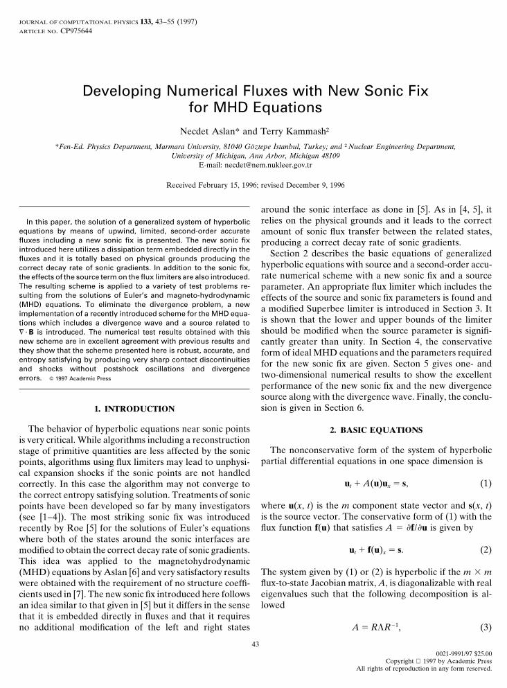
FIG. 9. Regular high-Mach reflection problem. Bx contours obtained by (a) a 7 3 7 eigensystem without the divergence source and (b) an 8 3

8 eigensystem with the source.

2. P. K. Sweby, High-resolution schemes using flux limiters for hyper-netic monopoles are created and the numerical iterationsbolic conservation laws, SIAM J. Numer. Anal. 21, 995 (1984).become unstable. Figure 9b gives the results on the same

3, B. van Leer, W. T. Lee, and K. G. Powell, Sonic point capturinggrid obtained with the 8 3 8 eigensystem and divergence(AIAA Paper 89-1945), AAIA J. 49, 235 (1983).source. As seen, the solution is excellent since there are

4. R. J. LeVeque, High-resolution finite volume methods on arbitraryno problems arising from the divergence condition and thegrids via wave propagation, J. Comput. Phys. 78, 36 (1988).

shock compression remains uniform (even after reflection).5. P. L. Roe, Sonic flux formulae, SIAM J. Sci. Statist. Comput. 13,

As a remark, it is noted that using a rotated Riemann solver 611 (1992).would improve these results which is the main objective of 6. N. Aslan, Computational Investigations of Ideal MHD Plasmas withsubsequent papers. Discontinuities, Ph.D. thesis (Nuclear Engineering Department, Uni-

versity of Michigan, 1993).6. CONCLUSION 7. A. Zachary and P. Colella, A higher-order Godunov method for

the equations of ideal magnetohydrodynamics, J. Comput. Phys. 99,341 (1992).The solution of hyperbolic equations with simple first-

8. Glaister, An Approximate Riemann Solver for Compressible Flowsorder upwind differencing produces errors that accumulatewith Axial Symmetry, Num. Anal. Report, 2/87 (Department of Math-in time and it produces unphysical expansion shocks whichematics, University of Reading, 1987).slow down the convergence. To handle this problem, a new

9. W. F. Noh, Errors for calculations of strong shocks using an artificialsonic fix that utilizes a dissipation term which is directlyviscosity and an artificial heat flux, J. Comput. Phys. 72, 78 (1978).embedded in the fluxes is described here. The fix is not

10. P. L. Roe, Characteristic-based schemes for the Euler equations,empirical but certainly relies on physical grounds produc-Annu. Rev. Fluid Mech. 18, 337 (1986).

ing the correct decay rate of sonic gradients. A new imple-11. P. L. Roe, Approximate Riemann solvers, parameter vectors, and

mentation of the source terms into the flux limiters is also difference schemes, J. Comput. Phys. 43, 357 (1981).discussed in detail. A wide variety of one- or two-dimen- 12. N. Aslan, Numerical solutions of one-dimensional MHD equations bysional test problems resulting from the solutions of Euler’s a fluctuation approach, Int. J. Numer. Methods Fluids 22, 569 (1996).equations and a new implementation of a recently intro- 13. R. J. LeVeque, Numerical methods for conservation laws, Lecturesduced scheme for the MHD equations are presented. The at ETH Zurich (1989).results show that the scheme with the new sonic fix along 14. Philip L. Roe, Some contributions to the modelling of discontinuous

flows, Lectures Appl. Math. 22, 163 (1985).with new source strengths is robust and accurate, producingrather sharp contact discontinuities and shocks without 15. N. Aslan and T. Kammash, Plasma dynamics in a magnetically insu-

lated target for inertial fusion, Fusion Technol. 26, 184 (1994).spurious oscillations. The scheme is currently being im-16. J. U. Brackbill and D. C. Barnes, The effect of nonzero = ? B onproved to include curvilinear geometries, quadrilateral

the numerical solution of the magnetohydrodynamic equations, J.grids with flux rotation, and triangular grids.Comput. Phys. 35, 426 (1980).

17 K. G. Powell, An Approximate Riemann Solver for Magnetohydrody-ACKNOWLEDGMENTSnamics (That Works in More Than One Dimension), ICASE ReportNo. 94-24 (Langley, VA, 1994).The support from NATO Collaborative studies (CRG-941130) is ac-

18. T. I. Gombosi, K. G. Powell, and D. L. De Zeeuw, Axisymmetricknowledged. This work is also supported by the NSF under Contractmodelling of cometary mass loading on an adaptively refined grid,INT95-148148 with the University of Michigan. The discussions with P.J. Geophys. Res. 99, A11, 21525 (1994).Roe, B. van Leer, and K. Powell are gratefully acknowledged.

19. P. Woodward and P. Colella, The numerical solution of two-dimen-sional fluid flow with strong shocks, J. Comput. Phys. 54, 115 (1984).REFERENCES

20. W. J. Rider, A review of approximate Riemann solvers with Godu-nov’s method in Lagrangian coordinates, Comput. Fluids 23, 3971. A. Harten, High-resolution schemes for hyperbolic conservation laws,

J. Comput. Phys. 49, 235 (1983). (1994).


21. G. Sod, A survey of several finite difference methods for systems of 23. N. Aslan, Numerical solutions of 2-D MHD equations by finite vol-ume method with quadrilateral cells, in Proceedings, Ninth Int. Conf.hyperbolic conservation laws, J. Comput. Phys. 27, 1 (1978).in Numerical Meth. in Laminar and Turbulent Flow, 1995, 9-2, 1633.22. M. Brio and C. C. Wu, An upwind differencing scheme for the equa-

tions of ideal magnetohydrodynamics, J. Comput. Phys. 75, 400 24. N. Aslan, Two dimensional solutions of MHD equations with adaptedRoe’s method, Int. J. Numer. Methods Fluids 23, 1 (1996).(1988).

Developing Numerical Fluxes with New Sonic Fix for MHD Equations

Documents

Transcript of Developing Numerical Fluxes with New Sonic Fix for MHD Equations