A Statistical Benchmark for BosonSampling

Mattia Walschaers,1, 2, ∗ Jack Kuipers,3, 4 Juan-Diego Urbina,3 Klaus Mayer,1

Malte Christopher Tichy,5 Klaus Richter,3 and Andreas Buchleitner1

1Physikalisches Institut, Albert-Ludwigs-Universitat Freiburg,Hermann-Herder-Str. 3, D-79104 Freiburg, Germany

2Instituut voor Theoretische Fysica, University of Leuven,Celestijnenlaan 200D, B-3001 Heverlee, Belgium

3Institut fur Theoretische Physik, Universitat Regensburg, D-93040 Regensburg, Germany4D-BSSE, ETH Zurich, Mattenstrasse 26, 4058 Basel, Switzerland

5Department of Physics and Astronomy, Aarhus University, Ny Munkegade 120, DK-8000 Aarhus, Denmark(Dated: November 3, 2014)

Computing the state of a quantum mechanical many-body system composed of indistinguishableparticles distributed over a multitude of modes is one of the paradigmatic test cases of computationalcomplexity theory: Beyond well-understood quantum statistical effects, the coherent superpositionof many-particle amplitudes rapidly overburdens classical computing devices - essentially by creatingextremely complicated interference patterns, which also challenge experimental resolution. With theadvent of controlled many-particle interference experiments, optical set-ups that can efficiently probemany-boson wave functions - baptised BosonSamplers - have therefore been proposed as efficientquantum simulators which outperform any classical computing device, and thereby challenge theextended Church-Turing thesis, one of the fundamental dogmas of computer science. However,as in all experimental quantum simulations of truly complex systems, there remains one crucialproblem: How to certify that a given experimental measurement record is an unambiguous result ofsampling bosons rather than fermions or distinguishable particles, or of uncontrolled noise? In thiscontribution, we describe a statistical signature of many-body quantum interference, which can beused as an experimental (and classically computable) benchmark for BosonSampling.

I. INTRODUCTION

As the world waits for the first universal and fully op-erational quantum computer [1], quantum informationscientists are eager to already show the power of quan-tum physics to perform computational tasks which areout of reach for a classical computer. Rather than de-signing devices that can perform a wide range of calcu-lations, machines which are specialised in specific taskshave joined the scope [2, 3]. Here, we focus on one type ofsuch devices, the BosonSamplers, which may hold the keyto falsifying the extended Church-Turing thesis [1, 4, 5].This conjecture, rooted in the early days of computer sci-ence, states that any efficient calculation performed by aphysical device can also be performed in polynomial timeon a classical computer. It is now proposed that all that isnecessary to falsify this foundational dogma of computerscience is a set of m photonic input modes, which areconnected to m output modes by a random photonic cir-cuit [2]. This immediately indicates why BosonSamplingattracts such attention, as these systems are experimen-tally in reach [6–11].

Since we are dealing with bosons, indistinguishableparticles, interesting physics arises when multiple parti-cles are simultaneously injected into the system [12–16].A schematic overview, indicating the essential ingredi-ents of a sampling device such as considered here, is pro-vided in Figure 1. BosonSampling essentially consists in

∗ mattia@itf.fys.kuleuven.be

Input Output

Correlators

U

Figure 1. Sketch of the system under consideration. From aset of input modes (here m = 12), four particles are injected(depicted in red). The particles traverse the system via thedepicted channels. At the crossings, different paths are inter-connected such that particles can travel on in each direction,thus leading to single-particle and many-body interference.The yellow zone of the setup is described by a unitary matrixU , which connects the input modes to the output modes. Theoutput signal is probabilistic in nature (hence different inten-sities of red), with its statistics governed by the many-bodyquantum state. The key object of this work, the C-dataset(see main text), is obtained by calculating the two-point cor-relations between different modes as depicted in green.

arX

iv:1

410.

8547

v1 [

quan

t-ph

] 3

0 O

ct 2

014

2

quantifying the probability of measuring an occupationvector ~y = (y1, . . . , ym) for the output modes, given thatthe initial mode occupation was ~x = (x1, . . . xm), wherexi and yi are the number of photons found in the ithinput and output mode, respectively. In the case withat most one photon per input mode, this probability is

given by p~x→~y =|perm U~x,~y|2∏m

i=1 yi!, where U~x,~y is the n × n

matrix, constructed from U , which describes how the noccupied input modes are connected to the selected out-put modes [13], and “perm” denotes the permanent [17].The latter lies at the heart of the contemporary inter-est in the BosonSampling problem: In order to evalu-ate the many-body wave function, and thus the samplingstatistics, we must calculate permanents. A permanent,however, is “hard” to compute, as there is no algorithmthat can do so in polynomial time [2, 17, 18]. Thus, theBosonSampler is a physical system that efficiently sam-ples bosons according to the bosonic many-body wavefunction, even though this many-body state cannot becalculated by a classical computer in polynomial time.Its realisation would in this perspective invalidate theextended Church-Turing thesis. This strength of Boson-Sampling apparently also implies a profound weakness:As it is impossible to compute the many-body wave func-tion, one cannot certify that a given experimental outputunambiguously stems from sampling bosons.

Rather than joining in the mathematical debate aboutthe similarity of BosonSampling to sampling over otherdistributions [19, 20] or setting a benchmark based onan analytically treatable instance outside the computa-tionally hard generic case [21], we here tackle the problemfrom a physics perspective inspired by statistical mechan-ics. Borrowing from the vast set of techniques applied inthis field, we study transport processes in scattering sys-tems (e.g. a photonic network), given by a unitary ma-trix U . We show that, by combining quantum optics withmethods found in statistical physics and random matrixtheory, it is indeed possible to identify signatures of gen-uine bosonic interference with manageable overhead.

II. STATISTICAL SIGNATURES OFINTERFERENCE

It must be stressed that the resulting many-body wavefunction of a scattering process, such as manifested in aBosonSampler, is determined by several factors. One condivide them into those which are of a statistical origin andthose which are dynamical in nature. The former concernall effects related to the quantum statistics (e.g. the Pauliexclusion principle), whereas the latter involve all sortsof interference effects. One can divide these interferencesinto the well-known single-particle interference [22], en-coded within the matrix U , which arises due to the wave-like nature of quantum transport [23–25], and the farmore difficult many-body interference [15, 16, 26]. Here,we shall study the sampling of various particle types –bosons, fermions, distinguishable particles and “simu-

lated bosons”– and explain how to efficiently distinguishbetween them. Distinguishable particles are the simplestof the considered species, as their signals are governedonly by single-particle interference. Transport processeswith bosons or fermions, in contrast, exhibit the entirerange of statistical and interference effects. As indistin-guishable particles, they obey quantum statistics (as dic-tated by the relevant algebra), which for two particles intwo modes either leads to bunching (bosons) [12] or anti-bunching (fermions) [27]. Similar effects have also beenobserved in larger setups, with more particles, and havehence been proposed as hallmarks for many-boson [28] ormany-fermion [29] behaviour. However, for larger setupsone expects a much richer phenomenology due to many-body interference [15]. For BosonSampling, bunching be-haviour as such is not a sufficient tool for certification,as it can easily be achieved by the so-called mean-fieldsampler [21] which was inspired by semiclassical models[30]. These devices are designed to replicate the bunch-ing behaviour by approximating the many-body outputstate by a macroscopically populated single-particle statewith random phases added. Averaging over the randomphases mimics boson-like bunching. However, all rel-ative phases are destroyed in the averaging procedureand therefore all many-body interference effects are van-quished. This type of sampling is easily simulated byMonte Carlo methods – hence we refer to such sampledparticles as “simulated bosons”– stressing the importanceof setting this type of sampling apart from the actualBosonSampling. This, however, can be done, since wehere introduce a method to successfully differentiate thetransport processes of all these different particle types.

III. RANDOM MATRIX METHODS

The scattering matrix U that describes the photoniccircuit in the BosonSampling setup is randomly sampledfrom the Haar measure [31–33]. Therefore it is only nat-ural to treat this problem in a framework of statistics andrandom matrix theory (RMT) [31, 34–37]. Often the lackof grasp on the statistical distribution of the full many-body wave function is put forth as the core of the certi-fication problem. Exhaustive statistical characterisationof the many-body state would require the full distribu-tion of permanents over the set of unitary matrices. Todate, only the first moment of this distribution is known[38] and it is not enough to provide certification, whilesufficiently precise higher order moments are out of reach[2] . The reason is that, in terms of the quantum state,permanents depend on high-order correlation functions.We, on the other hand, want to emphasise the giganticamount of information about the many-body state whichis within reach in the form of distributions of low-ordercorrelation functions.

In probability theory, the knowledge of all possible cor-relation functions implies full knowledge of the (joint)probability distribution itself. Therefore, correlation

3

functions play a central role in many probabilistic the-ories, from RMT [31] to quantum statistical mechanics[39]. In practical applications of RMT, such as occurin quantum chaos, the full joint probability distributionof many eigenvalues of a large random matrix is outof reach; however, a study of the statistics related totwo-point correlations is often sufficient to certify theRMT ensemble. Similarly, here, we do not know allcorrelation functions of the many-body quantum state.There is, however, a large set of correlation functionswhich are accessible (both theoretically and experimen-tally) [14, 38, 40]. Hence, the only relevant question iswhether this offers a sufficient amount of information onthe many-body states for the various particle types to bedistinguished. We show that the answer to the questionis affirmative.

IV. STATISTICAL BENCHMARKING

We propose the mode correlator [14], Cij = 〈ninj〉 −〈ni〉〈nj〉 (with ni = a∗i ai the bosonic number operator),which quantifies how the number of outgoing photonsin modes i and j are correlated (as indicated in Figure1), as a suitable quantity to differentiate particle types.The particle type is encrypted in the many-body out-put quantum state |φout〉, which shows up in Cij via theexpectation value 〈.〉 = 〈φout|.|φout〉. A single such cor-relator cannot (typically) offer much insight in the fullwave function, rather some characteristic behaviour willbecome apparent once a sufficiently large set of such cor-relators is considered. This type of dataset, which we fur-ther refer to as the C-dataset, is easily obtained in the ex-perimental setup: One must consider all possible choicesfor output modes, i, j ∈ 1, . . .m such that i < j, andfor each choice compute the correlation Cij between thenumber of particles sampled in the two modes. Now, fora single choice of input modes and hence a single n×munitary matrix Usub, the submatrix of U that describeshow the input modes are coupled to all possible outputmodes, we obtain a set of data on which we can do statis-tics.

Given Usub, it is possible to exactly numerically calcu-late the C-dataset for each particle type [14] (see Meth-ods). Although we can explore this numerically via his-tograms, moments and other statistical properties, it isfar from straightforward to get an analytical grasp ofits statistics. Ideally, we would like to predict the ex-act shape of the distribution, given the number of inputmodes m and the number of incoming particles n, butthis appears to be an unrealistic goal. Nevertheless, af-ter longwinded RMT calculations, we obtained analyticalpredictions for the first three moments of the set of possi-ble outcomes when varying Usub for fixed i and j (ratherthan fixing Usub and varying i and j). Although the dis-tributions are mathematically not exactly equivalent, wefind good agreement with numerics (for a more elaboratediscussion, see Methods).

BosonsDistinguishable

Fermions

-0.004 -0.003 -0.002 -0.001 0.000 0.0010

500

1000

1500

C = <NiN j> - <Ni><N j>

PHC

L

Simulated BosonsBosons

-0.003 -0.002 -0.001 0.000 0.0010

200

400

600

800

1000

C = <NiN j> - <Ni><N j>

PHC

L

Figure 2. Normalised histograms of the correlator data, ob-tained by computing Cij = 〈ninj〉 − 〈ni〉〈nj〉 for all possiblemode combinations, for a system with six particles and 120modes. Top panel, the histogram for bosonic correlators iscompared to data obtained with fermions or distinguishableparticles inserted instead of bosons. At the bottom, the his-tograms for bosons is compared to the result for simulatedbosons, see main text. All histograms are obtained from onesingle circuit, using the same input modes, thus implying thesame Usub.

For a generated C-dataset for the different particletypes, considering one fixed Usub for 120 output modesand six particles, the top panel in Figure 2 clearly shows aqualitative difference in the histograms for different par-ticle types. In contrast, the bottom panel of Figure 2 in-dicates that the histograms of the true bosons and theirsimulated counterparts bear a strong resemblance. Ob-viously, a quantitative understanding is essential to re-ally distinguish bosons from the other particle species.The second and third moment of the obtained correla-tor dataset can exactly provide us with such an insight.Obtaining these quantities involves averaging productsof components of unitary matrices, for which straightfor-ward (but tedious) combinatorics are used [36, 37].

4

V. DIFFERENTIATING PARTICLE SPECIES

To acquire the clearest distinction between differentparticle types, we propose the normalised mean (NM)– the first moment divided by n/m2, the coefficient ofvariation (CV ) – the standard deviation divided by themean – and skewness (S) [41] of the C-dataset as bench-marks. For these quantities, we have obtained an an-alytical RMT prediction in terms of mode and particlenumber, but as these expressions are rather longwinded,we present them in the Appedix. Since the dataset isgenerated for a single Usub, as explained before, we doexpect slight deviations from these RMT results. In Fig-ure 3, we show the theoretical predictions (solid lines) forNM , CV and S, for a sampler in which six particles wereinjected, as a function of the number of modes. In orderto quantify the deviations from the the RMT prediction,we sampled, for various numbers of modes, 500 differentUsub matrices, calculated the respective C-dataset and itsmoments, and indicated the resulting average coefficientof variation and skewness by a point. The error bars in-dicate the standard deviation from this mean value andthus quantify the typical spread of possible outcomes. Weshow here that for these parameters, even NM is fit toeffectively differentiate bosons, fermions and distinguish-able particles, the curves for simulated and true bosons,however, collapse. CV , on the other hand, is a trust-worthy quantity to distinguish true bosons from distin-guishable particles and even from simulated bosons. Theskewness S completes the certification that the particlesunder consideration are actually bosons.

We must emphasise that the curves of Figure 3 repre-sent the typical values for CV and S, and that it might bepossible to encounter a large deviation from such quanti-ties. Moreover, one might dwell into a parameter regimewhere such standard deviation bars overlap and henceit is unrealistic to certify the sampler with a single Usub

measurement. Luckily, a simple change of input modesimplies a change in Usub and hence it is feasible to gener-ate several C-datasets from one circuit. Figure 4 showsthe outcomes for various such Usub matrices as points,where the x-coordinate indicates the coefficient of varia-tion and the y-coordinate shows the skewness. The colourcoded sets of points for different particle types are all sep-arated from each other, showing clearly that they can bedistinguished. As is indicated in Figure 4, upon aver-aging over all the points in each cloud, one finds values(indicated by the red circles) which are very well esti-mated by the RMT predictions (indicated by the red tri-angles), thus providing a strong quantitative tool for suchcertification. This quality of the certification is furtherenhanced in large systems by noticing that the cloud isexpected to shrink with the effective number of scatter-ing events inside the array, namely the typical number ofcrossings between optical paths in Figure 1 (state of theart experiments have ' 20).

In Figure 3 we have indicated that bosons, fermionsand distinguishable particles can be identified by study-

50 100 150 200 250 300

-1.2

-1.1

-1.0

-0.9

-0.8

-0.7

m

NM

Bosons

Distinguishable

Fermions

Simulated Bosons

50 100 150 200 250 300

-1.1

-1.0

-0.9

-0.8

-0.7

-0.6

-0.5

mC

V

50 100 150 200 250 300

-2.5

-2.0

-1.5

-1.0

-0.5

m

S

Figure 3. The theoretical RMT predictions (solid lines) forthe normalised mean NM (top), the coefficient of variationCV (middle) and skewness S (bottom) of the C-dataset arecompared to the numerical NM , CV and S values of sampledC-datasets for six particles, as a function of the number ofmodes m. For mode numbers m = 20, 40, . . . , 300, we sampled500 matrices Usub, for each of which the normalised mean, thecoefficient of variation and skewness of the C-dataset werecalculated. For each mode number, the average normalisedmean, coefficient of variation and skewness are indicated bya dot. Additionally, the standard deviations of the obtainedNM , CV and S results are shown by error bars around thesedots.

ing the mean of the C-dataset. Furthermore, Figure 4shows that for a rather large number of modes and a largeset of sampled Usub matrices, we can classify all species.The method presented, however, does not require such anabundance of modes and samples since we can performadditional statistical analyses on the obtained cluster of

5

-1.2 -1.1 -1.0 -0.9 -0.8 -0.7 -0.6-3.5

-3.0

-2.5

-2.0

-1.5

-1.0

-0.5

0.0

CV

S

Bosons

Distinguishable

Fermions

Simulated Bosons

Analytical Predictions

Numerical Mean

Figure 4. For six particles, in 120 modes, the coefficient ofvariation and skewness were calculated for C-datasets of 500sampled Usub matrices, The points labeled “bosons”, “distin-guishable”, “fermions” and “simulated bosons”, each connectto one C-dataset of a sampled Usub, the points’ position onthe plot indicates the calculated coefficient of variation CVand skewness S. The black and white triangles mark theRMT predictions for these quantities. Finally, the black andwhite circles indicate the mean value of each cluster of all thepoints scattered of each particle type. These means coincidewith the RMT predictions, thus the black and white trianglesare hidden underneath the black and white circles.

data points. We emphasise this in Figure 5, where datapoints for only 20 samples of Usub matrices for m = 20are shown. We focus specifically on bosons (indicated byblue points), where for each sample the average is cal-culated (red dot) and the red ellipses indicate two andfour standard errors of the sample mean. The RMT pre-diction for bosons (a blue circle), with a slight bias, fallswithin the four standard errors, whereas the RMT pre-diction for simulated bosons (purple square) is well out-side this region. Thus, we can successfully differentiatetrue bosons from simulated bosons using the RMT-basedtechniques described here.

VI. CONCLUSIONS

As explained above, the suggested methods can beapplied in a broad variety of experimental setups, for awide range of particle numbers n and mode numbers m.Of course, smaller m lead to smaller C-datasets, makingit difficult to achieve statistical significance. In ournumerical studies, however, we successfully distinguishthe particle types for as few as 20 modes. A niceadvantage of our method as compared to [19] is that wecan certainly treat regimes where m < n5.1, we even canexplore regimes in which m ∼ O(n). However, as n andm grow, in Figure 3 the curves for true and simulatedbosons will approach one another to a distance of theorder O(1/n). As the limit 1/n→ 0 is the semi-classicallimit, where mean-field theory is exact, this is as such notsurprising. The similarity of the two curves essentiallyimplies that the statistics in the C-dataset is stronglydominated by the quantum statistics of the particlesand thus by the bosonic bunching. In this sense, we

−3.

0−

2.0

−1.

00.

0

−1.1 −1.0 −0.9 −0.8 −0.7

−3.

0−

2.0

−1.

00.

0

−1.1 −1.0 −0.9 −0.8 −0.7

CV

S

Figure 5. Four scatterplots, each containing 20 randomlysampled Usub matrices for six particles in m = 20 outputmodes, from which coefficient of variation CV and the skew-ness S of the bosonic C-dataset were calculated. The averageof the cloud is indicated (red dot) as are the two- and fourstandard error regions (small and large ellipsoid respectively).The RMT prediction for bosons is shown (large blue dot) tobe contained within the ellipses for each of the four samples.The RMT prediction for simulated bosons (purple square)falls well outside the four standard errors.

see a lot of potential in methods such as the one weemployed here, to further explore specific signaturesof many-body interference, e.g. by filtering out thebunching contributions to the statistics.

In summary, we demonstrated that, by measuring themode correlators Ci,j = 〈ninj〉 − 〈ni〉〈nj〉 for all possiblecombinations of outgoing modes, one holds the key tocertifying BosonSampling. The mean, the variance, andthe skewness of such a C-dataset are sufficient to iden-tify the sampled particles as either bosons, fermions ordistinguishable particles beyond reasonable doubt. Byvarying the chosen input channels, and thereby generat-ing multiple such datasets one can efficiently distinguishtrue bosons from simulated bosons – which are designedto replicate bunching behaviour – through the character-istic first moments of their respective distributions by us-ing the RMT predictions presented here, and comparingthem to numerically or experimentally obtained resultsafter averaging over the different C-datasets.

What is the consequence thereof for the extendedChurch-Turing thesis? Clearly, the capacity of any classi-cal computer will be quickly exhausted when confrontedwith the task to evaluate a many-body wave functionrepresented by a permanent, as soon as the number ofbosonic constituents and modes is large enough. How-ever, much as in the classical theory of gases or of chaotic(classical or quantum) systems, there are robust statisti-cal quantifiers which indeed can be handled, and whichare accessible in state of the art experiments. In thissense, a “thermodynamic” or “statistical” interpretationof the extended Church-Turing thesis will prevail.

6

Acknowledgements - M.W. would like to thank theGerman National Academic Foundation for financial sup-port. M.C.T. acknowledges financial support by the Dan-ish Council for Independent Research. K.M. and A.B.

acknowledge partial support through the COST ActionMP1006 ‘Fundamental Problems in Quantum Physics’,and by DFG. J.D.U. and K.R. acknowledge partial sup-port through DFG.

[1] M. A. Nielsen and I. L. Chuang, Quantum Computationand Quantum Information (Cambridge University Press,2010).

[2] S. Aaronson and A. Arkhipov, Theory of Computing 9,143 (2013).

[3] T. Lanting, A. J. Przybysz, A. Y. Smirnov, F. M.Spedalieri, M. H. Amin, A. J. Berkley, R. Harris, F. Al-tomare, S. Boixo, P. Bunyk, N. Dickson, C. Enderud,J. P. Hilton, E. Hoskinson, M. W. Johnson, E. Ladizin-sky, N. Ladizinsky, R. Neufeld, T. Oh, I. Perminov,C. Rich, M. C. Thom, E. Tolkacheva, S. Uchaikin, A. B.Wilson, and G. Rose, Phys. Rev. X 4, 021041 (2014).

[4] D. Deutsch, Proc. R. Soc. Lond. A 400, 97 (1985).[5] C. Moore and S. Mertens, The Nature of Computation

(Oxford University Press, 2011).[6] M. A. Broome, A. Fedrizzi, S. Rahimi-Keshari, J. Dove,

S. Aaronson, T. C. Ralph, and A. G. White, Science339, 794 (2013).

[7] A. Crespi, R. Osellame, R. Ramponi, D. J. Brod, E. F.Galvao, N. Spagnolo, C. Vitelli, E. Maiorino, P. Mat-aloni, and F. Sciarrino, Nat. Photon. 7, 545 (2013).

[8] T. C. Ralph, Nat. Photon. 7, 514 (2013).[9] N. Spagnolo, C. Vitelli, M. Bentivegna, D. J. Brod,

A. Crespi, F. Flamini, S. Giacomini, G. Milani, R. Ram-poni, P. Mataloni, R. Osellame, E. F. Galvao, andF. Sciarrino, Nat. Photon. 8, 615 (2014).

[10] J. B. Spring, B. J. Metcalf, P. C. Humphreys,W. S. Kolthammer, X.-M. Jin, M. Barbieri, A. Datta,N. Thomas-Peter, N. K. Langford, D. Kundys, J. C.Gates, B. J. Smith, P. G. R. Smith, and I. A. Walm-sley, Science 339, 798 (2013).

[11] M. Tillmann, B. Dakic, R. Heilmann, S. Nolte, A. Sza-meit, and P. Walther, Nat. Photon. 7, 540 (2013).

[12] C. K. Hong, Z. Y. Ou, and L. Mandel, Phys. Rev. Lett.59, 2044 (1987).

[13] M. C. Tichy, M. Tiersch, F. de Melo, F. Mintert, andA. Buchleitner, Phys. Rev. Lett. 104, 220405 (2010).

[14] K. Mayer, M. C. Tichy, F. Mintert, T. Konrad, andA. Buchleitner, Phys. Rev. A 83, 062307 (2011).

[15] M. C. Tichy, M. Tiersch, F. Mintert, and A. Buchleitner,New J. Phys. 14, 093015 (2012).

[16] Y.-S. Ra, M. C. Tichy, H.-T. Lim, O. Kwon, F. Mintert,A. Buchleitner, and Y.-H. Kim, PNAS 110, 1227 (2013).

[17] H. Minc, Permanents, Encyclopedia of Mathematics andits Applications. Vol. 6. (Addison-Wesley PublishingCompany., 1978).

[18] L. Troyansky and N. Tishby, Proc. Physics of Computing, 96 (1996).

[19] S. Aaronson and A. Arkhipov, arXiv:1309.7460 (2013).[20] C. Gogolin, M. Kliesch, L. Aolita, and J. Eisert,

arXiv:1306.3995 (2013).[21] M. C. Tichy, K. Mayer, A. Buchleitner, and K. Mølmer,

Phys. Rev. Lett. 113, 020502 (2014).[22] E. Akkermans and G. Montambaux, Mesoscopic Physics

of Electrons and Photons (Cambridge Univ. Press, 2007).

[23] F. Bloch, Z. Physik 52, 555 (1929).[24] Y. Aharonov, L. Davidovich, and N. Zagury, Phys. Rev.

A 48, 1687 (1993).[25] T. Scholak, T. Wellens, and A. Buchleitner,

arXiv:1409.5625 (2014).[26] T. Engl, J. Dujardin, A. Arguelles, P. Schlagheck,

K. Richter, and J. D. Urbina, Phys. Rev. Lett. 112,140403 (2014).

[27] T. Jeltes, J. M. McNamara, W. Hogervorst, W. Vassen,V. Krachmalnicoff, M. Schellekens, A. Perrin, H. Chang,D. Boiron, A. Aspect, and C. I. Westbrook, Nature 445,402 (2007).

[28] J. Carolan, J. D. A. Meinecke, P. Shadbolt, N. J. Russell,N. Ismail, K. Worhoff, T. Rudolph, M. G. Thompson,J. L. O’Brien, J. C. F. Matthews, and A. Laing, Nat.Photon. 8, 621 (2014).

[29] T. Rom, T. Best, D. van Oosten, U. Schneider, S. Folling,B. Paredes, and I. Bloch, Nature 444, 733 (2006).

[30] M. Chuchem, K. Smith-Mannschott, M. Hiller, T. Kot-tos, A. Vardi, and D. Cohen, Phys. Rev. A 82, 053617(2010).

[31] M. L. Mehta, Random matrices (Elsevier/Academicpress, Amsterdam, 2004).

[32] F. Mezzadri, Notices AMS 54, 592 (2007).[33] K. Zyczkowski and M. Kus, J. Phys. A: Math. Gen. 27,

4235 (1994).[34] S. Samuel, J. Math. Phys. 21, 2695 (1980).[35] P. A. Mello, J. Phys. A 23, 4061 (1990).[36] P. W. Brouwer and C. W. J. Beenakker, J. Math. Phys.

37, 4904 (1996).[37] G. Berkolaiko and J. Kuipers, J. Math. Phys. 54, 112103

(2013).[38] J.-D. Urbina, J. Kuipers, Q. Hummel, and K. Richter,

arXiv:1409.1558 (2014).[39] O. Bratteli and D. W. Robinson, Operator Algebras

and Quantum Statistical Mechanics: Equilibrium States.Models in Quantum Statistical Mechanics (Springer Sci-ence & Business Media, 1997).

[40] A. Peruzzo, M. Lobino, J. C. F. Matthews, N. Matsuda,A. Politi, K. Poulios, X.-Q. Zhou, Y. Lahini, N. Ismail,K. Worhoff, Y. Bromberg, Y. Silberberg, M. G. Thomp-son, and J. L. OBrien, Science 329, 1500 (2010).

[41] H. L. MacGillivray, Ann. Stat. 14, 994 (1986).[42] O. Bohigas, M. J. Giannoni, and C. Schmit, Phys. Rev.

Lett. 52, 1 (1984).

7

Appendix A: Correlators

Initially, let us present a short and slightly more technical introduction to the central objects that build up theC-dataset, the two-particle correlators. Given some pure quantum state |φ〉, these objects are defined as Cij =〈φ|ninj |φ〉 − 〈φ|ni|φ〉〈φ|nj |φ〉, the main goal of studying these object is to gain insight in the structure of states |φ〉,which results from the scattering of a many-particle Fock state in a system (one might think of a complicated network)which is described by a single-particle scattering matrix U (which we numerically generate following the algorithmdescribed in [32]). As we initially start from a Fock state for which modes q1, . . . , qn are populated by a single particle,we can describe the initial state |φin〉 in terms of creation operators a∗q (for creation in the qth mode) that act on thevacuum state |Ω〉, as

|φin〉 = a∗q1 . . . a∗qn |Ω〉. (A1)

Now, by traversing the system, the matrix U acts by connecting an input mode a∗q to all possible output modes a∗i

a∗q →m∑i=1

Uq,ia∗i (A2)

and thus we obtain that

|φ〉 =

m∑i1,...,in=1

Uq1,i1a∗i1 . . . Uqn,ina

∗in |Ω〉. (A3)

For bosons (B) and fermions (F), an application of the (anti)commutation relations, [ai, a∗j ]± = δij1, and a long but

straightforward computation leads to expressions for Cij :

CBij = −n∑k=1

Uqk,iUqk,jU∗qk,i

U∗qk,j +

n∑k 6=l=1

Uqk,iUql,jU∗qliU∗qk,j , (A4)

CFij = −n∑k=1

Uqk,iUqk,jU∗qk,i

U∗qk,j −n∑

k 6=l=1

Uqk,iUql,jU∗ql,iU∗qk,j . (A5)

In the case of distinguishable particles, one can in principle treat the particles in an independent fashion and thus aparticle starting in input mode q will be found in output mode i with a probability pq→i = |Ui,q|2. As the particlesare distinguishable, these probabilities are not influenced by the presence of other particles, and via simple probabilitytheory we now find that

CDij =

n∑k<l=1

(pqk→ipql→j + pqk→jpql→i)−n∑

k,l=1

pqk→ipql→j

= −n∑k=1

Uqk,iUqk,jU∗qk,i

U∗qk,j .

(A6)

Finally, simulated bosons behave similarly to distinguishable particles, with the sole exception that the initial stateis different and that (uniformly distributed) random phases are included over which one needs to average [21]. Weessentially sample distinguishable particles, which are inserted in the form of a single-particle state that superposes all

input modes with the same amplitude, but with random phases, implying a probability pi = 1n

∣∣∑nr=1 e

iθqrUqr,i∣∣2 to

find a particle in output mode i. Since every time we consider n such indistinguishable particles, a simple calculationyields

CSij = E(n(n− 1)pipj)− E(npi)E(npj) (A7)

where E(.) denotes averaging over the random phases θr. Performing the average, we eventually obtain

CSij =

(1− 1

n

) n∑r 6=s=1

Uqs,iUqr,jU∗qr,iU

∗qs,j −

1

n

n∑r,s=1

Uqr,iUqs,jU∗qr,iU

∗qs,j . (A8)

8

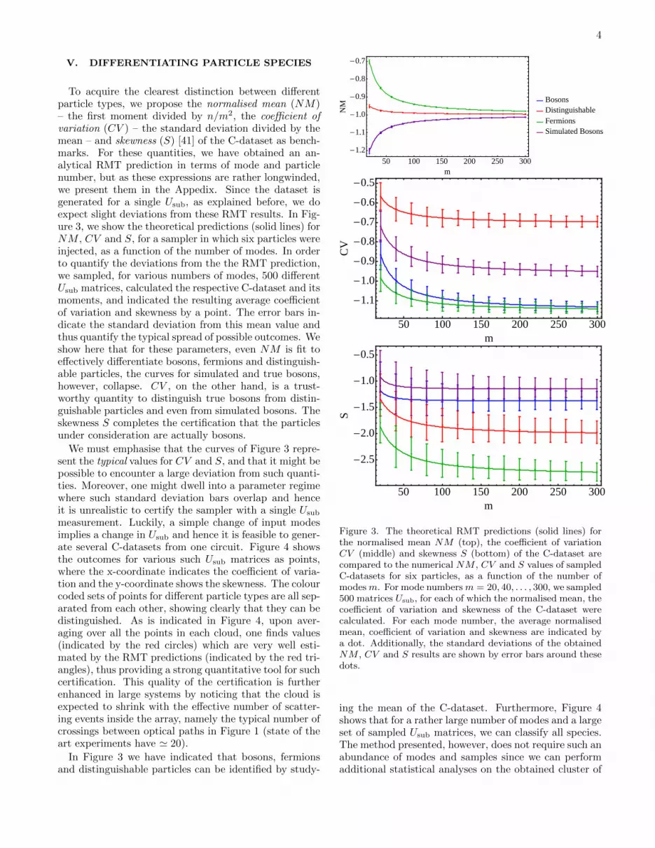
Appendix B: Random Matrix Theory

From expressions for the correlators of different particle types, we are able to construct the C-dataset by varying iand j (with i < j) to obtain all different mode combinations. In order to do theoretical predictions (or at least up tovery good approximation), we use RMT methods. Rather than varying i and j, these methods keep the two outputmodes under consideration fixed and formally average over all possible matrices U in the unitary group with the Haarmeasure imposed on it. One might understand this as an analogue to Bohigas-Giannoni-Schmit conjecture [42] forunitary matrices. The averaging contains one fundamental identity for an N ×N random unitary matrix U :

EU (Ua1,b1 . . . Uan,bnU∗α1,β1

. . . U∗αn,βn) =

∑σ,π∈Sn

VN (σ−1π)

n∏k=1

δ(ak − ασ(k))δ(bk − βπ(k)), (B1)

where EU (.) denotes the average over the unitary group and V are class coefficients also known as Weingartenfunctions, which are determined recursively, the details of this method can be found in [34–37]. With this formula,we efficiently average long products of coefficients of unitary matrices to compute EU (Cij), EU (C2

ij) and EU (C3ij) for

each particle type. Combining these quantities we can find the coefficient of variation CV and the skewness S foreach particle type. We find, with n particles in m modes, for bosons:

EU (CB) =n(−m− n+ 2)

m(m2 − 1), (B2)

EU(CB

2)

=2n(m2n+m2 + 9mn− 11m+ n3 − 2n2 + 5n− 4

)m2(m+ 2)(m+ 3)(m2 − 1)

, (B3)

EU(CB

3)

= −2n

(m3n2 + 15m3n+ 2m3 + 3m2n3 + 6m2n2 + 213m2n− 222m2 − 3mn4

m2(m+ 1)(m+ 2)(m+ 3)(m+ 4)(m+ 5)(m2 − 1)

+45mn3 + 32mn2 + 372mn− 464m+ 3n5 − 6n4 + 45n3 + 78n2 + 168n− 288

m2(m+ 1)(m+ 2)(m+ 3)(m+ 4)(m+ 5)(m2 − 1)

),

(B4)

for fermions

EU (CF ) =n(n−m)

m(m2 − 1), (B5)

EU(CF

2)

=2n(n+ 1)(m− n)(m− n+ 1)

m2(m+ 2)(m+ 3)(m2 − 1), (B6)

EU(CF

3)

= − 6n(n+ 1)(n+ 2)(m− n)(m− n+ 1)(m− n+ 2)

m2(m+ 1)(m+ 2)(m+ 3)(m+ 4)(m+ 5)(m2 − 1), (B7)

for distinguishable particles

EU (CD) = − n

m(m+ 1), (B8)

EU(CD

2)

=n(m2n+ 3m2 +mn− 5m+ 2n− 2

)m2(m+ 2)(m+ 3)(m2 − 1)

, (B9)

EU(CD

3)

= −n(m2n2 + 9m2n+ 26m2 + 5mn2 + 21mn− 62m+ 12n2 + 60n− 72

)m2(m+ 2)(m+ 3)(m+ 4)(m+ 5)(m2 − 1)

, (B10)

9

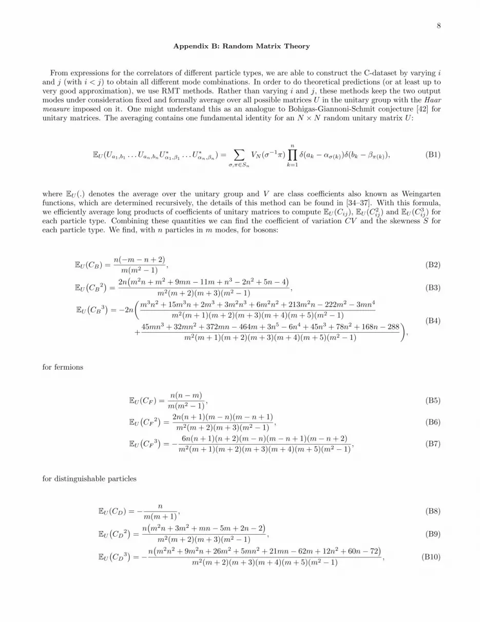
and finally for the simulated bosons

EU (CS) = −n(m+ n− 2)

m(m2 − 1), (B11)

EU(CS

2)

=4mn−m− 14n2 + 8n− 2

m2(m+ 2)(m+ 3)(m2 − 1)n

+2m2n3 −m2n2 + 4m2n−m2 + 18mn3 − 25mn2 + 2n5 − 4n4 + 10n3

m2(m+ 2)(m+ 3)(m2 − 1)n,

(B12)

EU(CS

3)

=

(−2m3n5 − 21m3n4 + 30m3n3 − 41m3n2 − 10m3n+ 8m3 − 6m2n6 − 3m2n5

(m− 1)m2(m+ 1)2(m+ 2)(m+ 3)(m+ 4)(m+ 5)n2

+−285m2n4 + 261m2n3 + 75m2n2 − 66m2n+ 24m2 + 6mn7 − 90mn6 − 55mn5

(m− 1)m2(m+ 1)2(m+ 2)(m+ 3)(m+ 4)(m+ 5)n2

+−360mn4 + 591mn3 + 8mn2 − 128mn+ 64m

(m− 1)m2(m+ 1)2(m+ 2)(m+ 3)(m+ 4)(m+ 5)n2

+−6n8 + 12n7 − 90n6 − 120n5 − 24n4 + 396n3 − 168n2 − 48(n− 1)

(m− 1)m2(m+ 1)2(m+ 2)(m+ 3)(m+ 4)(m+ 5)n2

).

(B13)

Although these formulas do not appear remarkably elegant due the lack of any form of assumption on m and n (apartfrom m > n), they are necessary to obtain sufficiently accurate results. Once these moments are defined, we can usethem to find NM , CV and S by the following definitions:

NM =EU (C)m2

n(B14)

CV =

√EU (C2)− EU (C)2

EU (C), (B15)

S =EU (C3)− 3EU (C)EU (C2) + 2EU (C)3

(EU (C2)− EU (C)2)3/2

. (B16)

With these results, one can now calculate the expected coefficient of variation and the expected skewness for each ofthe samplers we described, with an arbitrary number of modes and particles.