FMKe: A realistic benchmark for key-value stores - ASC
134
Gonçalo Alexandre Pinto Tomás Bachelor Degree in Sciences and Computer Engineering FMKe: A realistic benchmark for key-value stores Dissertation submitted in partial fulfillment of the requirements for the degree of Master of Science in Computer Science and Engineering Adviser: João Leitão, Assistant Professor, Faculdade de Ciências e Tecnologia da Universidade Nova de Lisboa Co-adviser: Nuno Preguiça, Associate Professor, Faculdade de Ciências e Tecnologia da Universidade Nova de Lisboa Examination Committee Chairperson: Jorge Carlos Ferreira Rodrigues da Cruz Raporteur: João Nuno de Oliveira e Silva December, 2018
-
Upload
khangminh22 -
Category
Documents
-
view
3 -
download
0
Transcript of FMKe: A realistic benchmark for key-value stores - ASC

Gonçalo Alexandre Pinto Tomás
Bachelor Degree in Sciences and Computer Engineering
FMKe: A realistic benchmark for key-value stores
Dissertation submitted in partial fulfillmentof the requirements for the degree of
Master of Science inComputer Science and Engineering
Adviser: João Leitão, Assistant Professor,Faculdade de Ciências e Tecnologia daUniversidade Nova de Lisboa
Co-adviser: Nuno Preguiça, Associate Professor,Faculdade de Ciências e Tecnologia daUniversidade Nova de Lisboa
Examination Committee
Chairperson: Jorge Carlos Ferreira Rodrigues da CruzRaporteur: João Nuno de Oliveira e Silva
December, 2018


FMKe: A realistic benchmark for key-value stores
Copyright © Gonçalo Alexandre Pinto Tomás, Faculty of Sciences and Technology, NOVA
University of Lisbon.
The Faculty of Sciences and Technology and the NOVA University of Lisbon have the
right, perpetual and without geographical boundaries, to file and publish this dissertation
through printed copies reproduced on paper or on digital form, or by any other means
known or that may be invented, and to disseminate through scientific repositories and
admit its copying and distribution for non-commercial, educational or research purposes,
as long as credit is given to the author and editor.
This document was created using the (pdf)LATEX processor, based in the “novathesis” template[1], developed at the Dep. Informática of FCT-NOVA [2].[1] https://github.com/joaomlourenco/novathesis [2] http://www.di.fct.unl.pt


To João, for teaching me how, and to Diana, Joaquim, Mónicaand Pati for being why.


Acknowledgements
This work would not have been possible without the help of several people to which I am
most grateful. First of all I have to thank my advisors, João Leitão and Nuno Preguiça, for
their continued support throughout the realization of this work. I am thankful to have
gotten an opportunity to work with them.
I want to thank Valter Balegas, Deepthi Akkoorath, Peter Zeller and Annette Bieniusa.
Their help with Erlang related questions and also with the design of the driver interfaces
made our implementation easier to use and maintain.
My gratitude extends, of course, to the Informatics Department of the NOVA Univer-
sity of Lisbon, in particular to the NOVA LINCS research center and its members, for
providing an excellent environment to work in. Despite having some experience with
other workplaces, I relish the memories of great camaraderie that I experienced while
working with many people from the Computer Systems group.
This work would not be possible without the financial support of some very important
research projects:
• SyncFree European Research Project, grant agreement ID 609551
• LightKone European Research Project, H2020 grant agreement ID 732505
• NG-STORAGE Portuguese Research Project, Financed by FCT/MCTES (contract
PTDC/CCI-INF/32038/2017)
• NOVA LINCS, financed by FCT/MCTES (grant UID/CEC/04516/2013)
Some colleagues and friends have also contributed to this work with their support
and ideas. I am thankful for the thoughtful suggestions and reviews of Bernardo Ferreira,
Guilherme Borges, Pedro Fouto and Pedro Ákos Costa.
Finally I would like to express my deepest thanks to my family for their enthusiastic
encouragement. In particular to my fiancée Diana who is a constant source of inspiration
and motivation.
vii


Abstract
Standard benchmarks are essential tools to evaluate and compare database management
systems in terms of relevant semantic properties and performance. They provide the
means to evaluate a system with workloads that mimic real applications. Although a num-
ber of realistic benchmarks already exist for relational database systems, the same cannot
be said for NoSQL databases. This latter class of data storage systems has become increas-
ingly relevant for geo-distributed systems, and this has led developers and researchers to
either rely on benchmarks that do not model realistic workloads or to adapt the aforemen-
tioned benchmarks for relational databases to work for NoSQL databases, in a somewhat
ad-hoc fashion. Since these benchmarks assume an isolation and transactional model in
the database, they are inherently inadequate to evaluate NoSQL databases.
In this thesis, we propose a new benchmark that addresses the lack of realistic eval-
uation tools for distributed key-value stores. We consider a workload that is based on
information we have acquired about a real world deployment of a large-scale applica-
tion that operates over a distributed key-value store, that is responsible for managing
patient prescriptions at a nation-wide level in Denmark. We design our benchmark to
be extensible to a wide range of distributed key-value storage systems and some rela-
tional database systems with minimal effort for programmers, which only need to design
and implement specific data storage drivers to benchmark different alternatives. We fur-
ther present a study on the performance of multiple database management systems in
different deployment scenarios.
Keywords: Benchmark, Key-Value Store
ix


Resumo
Os benchmarks são ferramentas essenciais para avaliar e comparar sistemas de gestão
de bases de dados relativamente às suas propriedades semânticas e desempenho. Estes
fornecem os meios para avaliar um sistema através da injeção sistemática de cargas de
trabalho que imitam aplicações reais. Embora já existam vários benchmarks realistas
para sistemas de gestão de bases de dados relacionais, o mesmo não se verifica para bases
de dados NoSQL. Esta última classe de sistemas de armazenamento de dados é cada
vez mais relevante para os sistemas geo-distribuídos, o que levou a que programadores e
investigadores recorressem a benchmarks que não possuem cargas de trabalho realistas ou
adaptassem os benchmarks para bases de dados relacionais para operarem sobre bases de
dados NoSQL. No entanto, como esses benchmarks assumem um modelo de isolamento
e transacional na base de dados, são inerentemente inadequados para avaliar uma base
de dados NoSQL.
Nesta tese propomos um novo benchmark que aborda a falta de ferramentas de ava-
liação realistas para sistemas de armazenamento chave-valor distribuídos. Para esse fim
recorremos a um gerador de operações que injeta carga sobre a base de dados a partir de
informação que obtivemos sobre uma instalação de uma aplicação real em larga escala,
que opera sobre um sistema de armazenamento chave-valor distribuídos responsável
pela administração de receitas de pacientes a nível nacional na Dinamarca. Desenhámos
o nosso benchmark para ser extensível a uma ampla gama de sistemas de armazenamento
chave-valor distribuídos e algumas bases de dados relacionais com um esforço mínimo
para programadores, que só precisam desenhar e implementar drivers específicos para
avaliar as suas soluções. Finalmente, apresentamos um estudo do desempenho de múlti-
plos sistemas de gestão de bases de dados em diferentes cenários de instalação.
Palavras-chave: Benchmark, Bases de Dados Chave-Valor
xi


Contents
List of Figures xvii
List of Tables xix
Listings xxi
1 Introduction 1
1.1 Motivation . . . . . . . . . . . . . . . . . . . . . . . . . . . . . . . . . . . . 1
1.2 Problem Definition . . . . . . . . . . . . . . . . . . . . . . . . . . . . . . . 3
1.3 Contributions . . . . . . . . . . . . . . . . . . . . . . . . . . . . . . . . . . 3
1.4 Publications . . . . . . . . . . . . . . . . . . . . . . . . . . . . . . . . . . . 4
1.5 Structure of the Document . . . . . . . . . . . . . . . . . . . . . . . . . . . 4
2 Related Work 7
2.1 Databases . . . . . . . . . . . . . . . . . . . . . . . . . . . . . . . . . . . . . 7
2.2 Relational Databases . . . . . . . . . . . . . . . . . . . . . . . . . . . . . . 8
2.2.1 Data Model . . . . . . . . . . . . . . . . . . . . . . . . . . . . . . . 8
2.2.2 Programmer Interface . . . . . . . . . . . . . . . . . . . . . . . . . 9
2.2.3 Relevant Examples and Usage . . . . . . . . . . . . . . . . . . . . . 12
2.2.4 Distributed Relational Databases . . . . . . . . . . . . . . . . . . . 12
2.3 NoSQL Databases . . . . . . . . . . . . . . . . . . . . . . . . . . . . . . . . 14
2.3.1 Data Model . . . . . . . . . . . . . . . . . . . . . . . . . . . . . . . 14
2.3.2 Data Replication and Consistency . . . . . . . . . . . . . . . . . . . 15
2.3.3 Common Replication Strategies for NoSQL Databases . . . . . . . 16
2.3.4 Availability versus Consistency . . . . . . . . . . . . . . . . . . . . 16
2.3.5 Programmer Interface . . . . . . . . . . . . . . . . . . . . . . . . . 17
2.3.6 Relevant Examples . . . . . . . . . . . . . . . . . . . . . . . . . . . 18
2.4 Database Benchmarks . . . . . . . . . . . . . . . . . . . . . . . . . . . . . . 19
2.4.1 Benchmarks for Relational Databases . . . . . . . . . . . . . . . . . 20
2.4.2 Benchmarks for NoSQL Databases . . . . . . . . . . . . . . . . . . 21
2.4.3 Benchmark Adaptations . . . . . . . . . . . . . . . . . . . . . . . . 22
2.5 Conflict-free Replicated Data Types . . . . . . . . . . . . . . . . . . . . . . 22
2.5.1 Replication Strategies . . . . . . . . . . . . . . . . . . . . . . . . . . 23
xiii

CONTENTS
2.5.2 Data Types . . . . . . . . . . . . . . . . . . . . . . . . . . . . . . . . 25
2.5.3 Discussion . . . . . . . . . . . . . . . . . . . . . . . . . . . . . . . . 25
2.6 Summary . . . . . . . . . . . . . . . . . . . . . . . . . . . . . . . . . . . . . 26
3 The FMKe Benchmark 27
3.1 Overview . . . . . . . . . . . . . . . . . . . . . . . . . . . . . . . . . . . . . 27
3.2 Architecture . . . . . . . . . . . . . . . . . . . . . . . . . . . . . . . . . . . 28
3.3 Benchmark Design . . . . . . . . . . . . . . . . . . . . . . . . . . . . . . . 30
3.4 Data Model . . . . . . . . . . . . . . . . . . . . . . . . . . . . . . . . . . . . 31
3.4.1 Relational Data Model . . . . . . . . . . . . . . . . . . . . . . . . . 32
3.4.2 Denormalised Data Model . . . . . . . . . . . . . . . . . . . . . . . 33
3.4.3 Data Model Performance Comparison . . . . . . . . . . . . . . . . 34
3.5 Application Level Operations . . . . . . . . . . . . . . . . . . . . . . . . . 35
3.5.1 Create Patient . . . . . . . . . . . . . . . . . . . . . . . . . . . . . . 36
3.5.2 Create Pharmacy . . . . . . . . . . . . . . . . . . . . . . . . . . . . 36
3.5.3 Create Facility . . . . . . . . . . . . . . . . . . . . . . . . . . . . . . 37
3.5.4 Create Medical Staff . . . . . . . . . . . . . . . . . . . . . . . . . . . 37
3.5.5 Create Prescription . . . . . . . . . . . . . . . . . . . . . . . . . . . 38
3.5.6 Get Patient By Id . . . . . . . . . . . . . . . . . . . . . . . . . . . . 39
3.5.7 Get Pharmacy By Id . . . . . . . . . . . . . . . . . . . . . . . . . . . 39
3.5.8 Get Facility By Id . . . . . . . . . . . . . . . . . . . . . . . . . . . . 40
3.5.9 Get Staff By Id . . . . . . . . . . . . . . . . . . . . . . . . . . . . . . 40
3.5.10 Get Prescription By Id . . . . . . . . . . . . . . . . . . . . . . . . . 41
3.5.11 Get Pharmacy Prescriptions . . . . . . . . . . . . . . . . . . . . . . 41
3.5.12 Get Processed Pharmacy Prescriptions . . . . . . . . . . . . . . . . 42
3.5.13 Get Prescription Medication . . . . . . . . . . . . . . . . . . . . . . 42
3.5.14 Get Staff Prescriptions . . . . . . . . . . . . . . . . . . . . . . . . . 43
3.5.15 Update Patient Details . . . . . . . . . . . . . . . . . . . . . . . . . 43
3.5.16 Update Pharmacy Details . . . . . . . . . . . . . . . . . . . . . . . 44
3.5.17 Update Facility Details . . . . . . . . . . . . . . . . . . . . . . . . . 44
3.5.18 Update Staff Details . . . . . . . . . . . . . . . . . . . . . . . . . . . 45
3.5.19 Update Prescription Medication . . . . . . . . . . . . . . . . . . . . 45
3.5.20 Process Prescription . . . . . . . . . . . . . . . . . . . . . . . . . . 46
3.6 Consistency Requirements Analysis . . . . . . . . . . . . . . . . . . . . . . 46
3.7 Workload . . . . . . . . . . . . . . . . . . . . . . . . . . . . . . . . . . . . . 47
3.8 Summary . . . . . . . . . . . . . . . . . . . . . . . . . . . . . . . . . . . . . 49
4 FMKe Implementation 51
4.1 Software Packages . . . . . . . . . . . . . . . . . . . . . . . . . . . . . . . . 52
4.1.1 Application Server . . . . . . . . . . . . . . . . . . . . . . . . . . . 52
4.1.2 Load Generation Tool . . . . . . . . . . . . . . . . . . . . . . . . . . 55
xiv

CONTENTS
4.1.3 Database Population Utility . . . . . . . . . . . . . . . . . . . . . . 57
4.2 FMKe Driver Interface . . . . . . . . . . . . . . . . . . . . . . . . . . . . . 57
4.2.1 Generic Driver . . . . . . . . . . . . . . . . . . . . . . . . . . . . . . 57
4.2.2 Optimized Driver . . . . . . . . . . . . . . . . . . . . . . . . . . . . 58
4.2.3 Driver Interface Comparison . . . . . . . . . . . . . . . . . . . . . 59
4.3 Supported Systems . . . . . . . . . . . . . . . . . . . . . . . . . . . . . . . 60
4.4 Summary . . . . . . . . . . . . . . . . . . . . . . . . . . . . . . . . . . . . . 60
5 Experimental Evaluation 61
5.1 AntidoteDB Performance Study . . . . . . . . . . . . . . . . . . . . . . . . 61
5.1.1 Test Environment . . . . . . . . . . . . . . . . . . . . . . . . . . . . 62
5.1.2 Benchmark Procedure . . . . . . . . . . . . . . . . . . . . . . . . . 63
5.1.3 Driver Versions . . . . . . . . . . . . . . . . . . . . . . . . . . . . . 64
5.1.4 Cluster Size . . . . . . . . . . . . . . . . . . . . . . . . . . . . . . . 65
5.1.5 Multiple Data-centers . . . . . . . . . . . . . . . . . . . . . . . . . 65
5.2 Comparative Performance Study . . . . . . . . . . . . . . . . . . . . . . . . 66
5.2.1 Test Environment . . . . . . . . . . . . . . . . . . . . . . . . . . . . 67
5.2.2 Benchmark Procedure . . . . . . . . . . . . . . . . . . . . . . . . . 67
5.2.3 Database Configuration . . . . . . . . . . . . . . . . . . . . . . . . 67
5.2.4 Performance Analysis . . . . . . . . . . . . . . . . . . . . . . . . . . 69
5.3 Discussion . . . . . . . . . . . . . . . . . . . . . . . . . . . . . . . . . . . . 75
5.4 Summary . . . . . . . . . . . . . . . . . . . . . . . . . . . . . . . . . . . . . 76
6 Conclusions and Future Work 79
6.1 Conclusions . . . . . . . . . . . . . . . . . . . . . . . . . . . . . . . . . . . 79
6.2 Future Work . . . . . . . . . . . . . . . . . . . . . . . . . . . . . . . . . . . 80
Bibliography 81
A CQL Table Creation Statements 87
B AntidoteDB Performance Results 89
B.1 32 Clients . . . . . . . . . . . . . . . . . . . . . . . . . . . . . . . . . . . . . 90
B.2 64 Clients . . . . . . . . . . . . . . . . . . . . . . . . . . . . . . . . . . . . . 91
B.3 128 Clients . . . . . . . . . . . . . . . . . . . . . . . . . . . . . . . . . . . . 92
B.4 256 Clients . . . . . . . . . . . . . . . . . . . . . . . . . . . . . . . . . . . . 93
B.5 512 Clients . . . . . . . . . . . . . . . . . . . . . . . . . . . . . . . . . . . . 94
C Cassandra Performance Results 95
C.1 32 Clients . . . . . . . . . . . . . . . . . . . . . . . . . . . . . . . . . . . . . 96
C.2 64 Clients . . . . . . . . . . . . . . . . . . . . . . . . . . . . . . . . . . . . . 97
C.3 128 Clients . . . . . . . . . . . . . . . . . . . . . . . . . . . . . . . . . . . . 98
C.4 256 Clients . . . . . . . . . . . . . . . . . . . . . . . . . . . . . . . . . . . . 99
xv

CONTENTS
C.5 512 Clients . . . . . . . . . . . . . . . . . . . . . . . . . . . . . . . . . . . . 100
D Redis Cluster Performance Results 101
D.1 32 Clients . . . . . . . . . . . . . . . . . . . . . . . . . . . . . . . . . . . . . 102
D.2 64 Clients . . . . . . . . . . . . . . . . . . . . . . . . . . . . . . . . . . . . . 103
D.3 128 Clients . . . . . . . . . . . . . . . . . . . . . . . . . . . . . . . . . . . . 104
D.4 256 Clients . . . . . . . . . . . . . . . . . . . . . . . . . . . . . . . . . . . . 105
D.5 512 Clients . . . . . . . . . . . . . . . . . . . . . . . . . . . . . . . . . . . . 106
E Riak Performance Results 107
E.1 32 Clients . . . . . . . . . . . . . . . . . . . . . . . . . . . . . . . . . . . . . 108
E.2 64 Clients . . . . . . . . . . . . . . . . . . . . . . . . . . . . . . . . . . . . . 109
E.3 128 Clients . . . . . . . . . . . . . . . . . . . . . . . . . . . . . . . . . . . . 110
E.4 256 Clients . . . . . . . . . . . . . . . . . . . . . . . . . . . . . . . . . . . . 111
E.5 512 Clients . . . . . . . . . . . . . . . . . . . . . . . . . . . . . . . . . . . . 112
xvi

List of Figures
2.1 Visual representation of a table in the Relational Model . . . . . . . . . . . . 8
2.2 Visual representation of the CAP theorem . . . . . . . . . . . . . . . . . . . . 16
2.3 CRDT Set Example: Last Writer Wins policy may cause loss of data. . . . . . 23
2.4 State Based Set: Example of state merge between two server replicas containing
different values. . . . . . . . . . . . . . . . . . . . . . . . . . . . . . . . . . . . 24
2.5 Operation Based Set: Example of operation based merge between two server
replicas containing different values. . . . . . . . . . . . . . . . . . . . . . . . . 25
3.1 FMK Entity-Relation Diagram . . . . . . . . . . . . . . . . . . . . . . . . . . . 28
3.2 FMKe Architecture . . . . . . . . . . . . . . . . . . . . . . . . . . . . . . . . . 29
3.3 Nested Data Model Example: Patient Prescription . . . . . . . . . . . . . . . 33
3.4 Denormalized Data Model Example: Patient Prescription . . . . . . . . . . . 34
3.5 Performance comparison of the nested and denormalized data models for the
ETS built-in key-value store . . . . . . . . . . . . . . . . . . . . . . . . . . . . 35
4.1 Application Server Directory Tree . . . . . . . . . . . . . . . . . . . . . . . . . 52
4.2 Workload Generator Directory Tree . . . . . . . . . . . . . . . . . . . . . . . . 56
4.3 Benchmark Result for AntidoteDB in a 4-node cluster with 32 clients . . . . 56
4.4 Performance comparison of a simple and optimized drivers for the same database 59
5.1 Architecture for a large single cluster experiment. AntidoteDB does not repli-
cate data in a single cluster. . . . . . . . . . . . . . . . . . . . . . . . . . . . . 62
5.2 Throughput over latency plot for different driver versions . . . . . . . . . . . 64
5.3 Throughput over latency plots for varying cluster size . . . . . . . . . . . . . 65
5.4 Throughput over latency plot for varying number of data-centers . . . . . . . 66
5.5 Throughput over latency plot using 128 clients . . . . . . . . . . . . . . . . . 70
5.6 Throughput over latency plot using 64 clients . . . . . . . . . . . . . . . . . . 71
5.7 Throughput over latency plot using 128 clients . . . . . . . . . . . . . . . . . 72
5.8 Throughput over latency plot using 64 clients . . . . . . . . . . . . . . . . . . 73
5.9 Average throughput for all FMKe drivers . . . . . . . . . . . . . . . . . . . . . 74
5.10 Minimum observed throughput over average latency . . . . . . . . . . . . . . 74
5.11 Maximum observed throughput over average latency . . . . . . . . . . . . . . 75
xvii

List of Figures
B.1 Throughput over latency plot using 32 clients . . . . . . . . . . . . . . . . . . 90
B.2 Throughput over latency plot using 64 clients . . . . . . . . . . . . . . . . . . 91
B.3 Throughput over latency plot using 128 clients . . . . . . . . . . . . . . . . . 92
B.4 Throughput over latency plot using 256 clients . . . . . . . . . . . . . . . . . 93
B.5 Throughput over latency plot using 512 clients . . . . . . . . . . . . . . . . . 94
C.1 Throughput over latency plot using 32 clients . . . . . . . . . . . . . . . . . . 96
C.2 Throughput over latency plot using 64 clients . . . . . . . . . . . . . . . . . . 97
C.3 Throughput over latency plot using 128 clients . . . . . . . . . . . . . . . . . 98
C.4 Throughput over latency plot using 256 clients . . . . . . . . . . . . . . . . . 99
C.5 Throughput over latency plot using 512 clients . . . . . . . . . . . . . . . . . 100
D.1 Throughput over latency plot using 32 clients . . . . . . . . . . . . . . . . . . 102
D.2 Throughput over latency plot using 64 clients . . . . . . . . . . . . . . . . . . 103
D.3 Throughput over latency plot using 128 clients . . . . . . . . . . . . . . . . . 104
D.4 Throughput over latency plot using 256 clients . . . . . . . . . . . . . . . . . 105
D.5 Throughput over latency plot using 512 clients . . . . . . . . . . . . . . . . . 106
E.1 Throughput over latency plot using 32 clients . . . . . . . . . . . . . . . . . . 108
E.2 Throughput over latency plot using 64 clients . . . . . . . . . . . . . . . . . . 109
E.3 Throughput over latency plot using 128 clients . . . . . . . . . . . . . . . . . 110
E.4 Throughput over latency plot using 256 clients . . . . . . . . . . . . . . . . . 111
E.5 Throughput over latency plot using 512 clients . . . . . . . . . . . . . . . . . 112
xviii

List of Tables
3.1 FMK operation frequency. Operations marked with * are read-only. . . . . . 30
3.2 FMKe Entity Attributes . . . . . . . . . . . . . . . . . . . . . . . . . . . . . . . 31
3.3 FMKe operations, along with their frequency. Operations marked with * are
read-only. . . . . . . . . . . . . . . . . . . . . . . . . . . . . . . . . . . . . . . . 48
xix


Listings
2.1 SQL Select Example Statement . . . . . . . . . . . . . . . . . . . . . . . . . 9
2.2 SQL Average Computation Example . . . . . . . . . . . . . . . . . . . . . 10
2.3 SQL Insert Example Statement . . . . . . . . . . . . . . . . . . . . . . . . . 10
2.4 SQL Update Statement . . . . . . . . . . . . . . . . . . . . . . . . . . . . . 10
2.5 SQL Delete Statement . . . . . . . . . . . . . . . . . . . . . . . . . . . . . . 10
2.6 SQL Transaction Example . . . . . . . . . . . . . . . . . . . . . . . . . . . 11
3.1 FMKe Table Creation SQL Statements . . . . . . . . . . . . . . . . . . . . . 32
3.2 Create Patient SQL Transaction . . . . . . . . . . . . . . . . . . . . . . . . 36
3.3 Create Pharmacy SQL Transaction . . . . . . . . . . . . . . . . . . . . . . . 36
3.4 Create Facility SQL Transaction . . . . . . . . . . . . . . . . . . . . . . . . 37
3.5 Create Staff SQL Transaction . . . . . . . . . . . . . . . . . . . . . . . . . . 37
3.6 Create Prescription Stored Procedure . . . . . . . . . . . . . . . . . . . . . 38
3.7 Get Patient By Id SQL Transaction . . . . . . . . . . . . . . . . . . . . . . . 39
3.8 Get Pharmacy By Id SQL Transaction . . . . . . . . . . . . . . . . . . . . . 39
3.9 Get Facility By Id SQL Transaction . . . . . . . . . . . . . . . . . . . . . . 40
3.10 Get Staff By Id SQL Transaction . . . . . . . . . . . . . . . . . . . . . . . . 40
3.11 Get Prescription By Id SQL Transaction . . . . . . . . . . . . . . . . . . . . 41
3.12 Get Pharmacy Prescriptions SQL Transaction . . . . . . . . . . . . . . . . 41
3.13 Get Processed Pharmacy Prescriptions SQL Transaction . . . . . . . . . . 42
3.14 Get Prescription Medication SQL Transaction . . . . . . . . . . . . . . . . 42
3.15 Get Staff Prescriptions SQL Transaction . . . . . . . . . . . . . . . . . . . 43
3.16 Update Patient Details SQL Transaction . . . . . . . . . . . . . . . . . . . 43
3.17 Update Pharmacy Details SQL Transaction . . . . . . . . . . . . . . . . . . 44
3.18 Update Facility Details SQL Transaction . . . . . . . . . . . . . . . . . . . 44
3.19 Update Staff Details SQL Transaction . . . . . . . . . . . . . . . . . . . . . 45
3.20 Update Prescription Medication SQL Transaction . . . . . . . . . . . . . . 45
3.21 Process Prescription SQL Transaction . . . . . . . . . . . . . . . . . . . . . 46
4.1 FMKe Configuration File . . . . . . . . . . . . . . . . . . . . . . . . . . . . 53
5.1 Cassandra FMKe keyspace . . . . . . . . . . . . . . . . . . . . . . . . . . . 68
A.1 Cassandra Table Creation Script . . . . . . . . . . . . . . . . . . . . . . . . 87
xxi


Chapter
1Introduction
1.1 Motivation
Database Management Systems (DBMS) are becoming ubiquitous in today’s society. As
companies and governments transition to digital storage of information and documents,
almost every new software project requires some form of persistent data storage. A
DBMS also provides easy access to data while abstracting away complex issues related
with efficiently retrieving data, processing transactions, recovering from crashes, etc.
In recent decades, developers have been given plenty of choices for databases: we’ve
seen the rise and widespread adoption of projects like MySQL, PostgreSQL, among many
others. The companies developing databases that respect the SQL standard provide typ-
ical features, such as transactional support, materialized views, programable functions
and triggers, secondary indexes, among others. Some DBMS however use slightly differ-
ent implementations for those different features which sometimes might not be publicly
documented and specified. This leads to an issue for software developers and software
project managers when it comes to selecting the most adequate storage system for their
applications or projects, since it is extremely difficult to compare the performance of
these different solutions.
Despite offering similar features, implementations vary across different storage sys-
tems and this leads to claims of significant performance differences between database
management systems. Fairly comparing database systems in an easy and fair way is a
non-trivial task, as results may become biased for a plethora of reasons. Even with a fixed
environment and dataset, different workloads with distinct data access patterns may show
significant performance deltas between storage systems, particularly if the database has
been optimized for a particular workload (e.g. read intensive, low write workload). A fair
comparison thus requires multiple scenarios, preferably guided by typical application
1

CHAPTER 1. INTRODUCTION
patterns. Additionally, to ensure that testing can uncover existing performance trade-offs,
it is essential to monitor multiple performance indicators.
The multiple challenges discussed above resulted in the establishment of the Trans-
action Processing Council (TPC), which for many years has taken the responsibility of
developing and specifying benchmarks for relational database management systems, that
can be used to systematically exercise the operations of databases and compare their per-
formance through the use of workloads inspired by real world use cases. The benchmarks
designed by the TPC have been widely adopted and are considered a standard for the
performance evaluation of this specific subset of data storage systems [31].
The release of the Amazon Dynamo [20] and the Yahoo’s PNUTS [18] systems marked
the first steps for a new, and relevant, type of data storage systems: distributed key
value stores. These new types of databases offered a simpler interface than conventional
DBMS while explicitly departing from the relational model and not supporting SQL-
like languages, leading to their famous “NoSQL” classification. Many projects based on
PNUTS and Dynamo have meanwhile emerged with some success in the market (e.g.
Riak [39], Cassandra [8], CouchDB [10]). This new class of databases started to see wide
adoption particularly in the context of web applications [20]. In fact, the design of these
DBMS was highly motivated by the need to provide low latency in large scale deployments
that span multiple data-centers, where the requirement of low latency for clients around
the globe is more important than the semantics provided by relational databases.
After several NoSQL databases were released, there was again a need to compare the
performance between different design and implementation strategies. In 2010, Yahoo
released a benchmark called the Yahoo Cloud Serving Benchmark (YCSB) [19] that was
designed for distributed key-value stores, which became widely adopted and quickly
considered the standard for this class of databases. Aside from being adapted for key-
value stores, YCSB still had a fundamental difference from the TPC benchmarks: its
workload consisted of synthetic read/write operations, while in the TPC benchmarks
the workload mimicked real world application patterns. While YCSB is considered a
very good baseline performance benchmark for key-value stores, this benchmark still
lacks somewhat in providing workloads that successfully emulate more sophisticated
and realistic application patterns.
The fact that YCSB only provides synthetic workloads, has lead many researchers to
rely on their own ad-hoc adaptations of TPC benchmarks for key-value stores [1, 37, 41].
This leads to experimental results that are hard to validate, compare, and reproduce.
We thus identify a need for a benchmark that simultaneously targets distributed key-
value stores and is based on a realistic application, which we try to address with the work
presented in this thesis.
2

1.2. PROBLEM DEFINITION
1.2 Problem Definition
In the thesis we propose to tackle the existing limitations of benchmarks for distributed
key-value stores, and design a solution that can, on the one hand, provide a systematic
way to evaluate and compare the performance benefits of different distributed key-value
stores, and on the other hand rely on a realistic use case with operations that illustrate a
realistic and interesting data access pattern. To this end we will base our work on informa-
tion that we have acquired regarding a realistic use case for distributed key value stores,
in particular the Fælles Medicinkort (FMK) system which is responsible for managing
patient prescriptions at a nation-wide level in Denmark.
Our benchmark, that we name FMKe, features multiple representative workloads of
the original system, that can be parameterized by the user in order to control the size of
the dataset, and the (average) amount of conflicting operations, among others. Moreover,
the benchmark is suitable to experimentally assess the performance of distributed key-
value stores in single site deployments and in geo-replicated deployment, which are both
extremely relevant nowadays.
Furthermore, and to ease the wide adoption of our benchmark, we designed it to be
extensible to a wide range of distributed key-value storage systems as well as relational
databases. This can be achieved through the implementation of (application-level) drivers
that transparently translate a generic specification of the operation in the FMK representa-
tive workloads into the concrete operation offered by the storage system. By allowing the
implementation of relational database drivers we hope to allow not only a performance
comparison between different distributed key-value stores, but also a contrast with re-
lational systems in order to determine whether the difference in performance justifies
the increase in complexity that is associated with the use of NoSQL databases as well as
the loss of commonly used features in relational storage systems such as transactional
support, materialized views, etc.
1.3 Contributions
This work presents two main contributions:
• An extensible benchmark that can be used to assess the performance of both NoSQL
and relational databases, which will allow programmers to verify which database
is most adequate to their use case from a performance standpoint. The benchmark
is readily available [23] as a set of software packages along with appropriate docu-
mentation.
• A comparative study of the performance of several different databases across dif-
ferent deployments. This study, to the best of our knowledge, represents the first
performance comparison of multiple NoSQL databases using a realistic benchmark.
3

CHAPTER 1. INTRODUCTION
1.4 Publications
Two publications have been made in the context of this thesis:
• Gonçalo Tomás, Peter Zeller, Valter Balegas, Deepthi Akkoorath, Annette Bieniusa,
João Leitão, and Nuno Preguiça. 2017. FMKe: A Real-World Benchmark for Key-Value Data Stores. In Proceedings of the 3rd International Workshop on Principles
and Practice of Consistency for Distributed Data (PaPoC ’17), Annette Bieniusa
and Alexey Gotsman (Eds.). ACM, New York, NY, USA, Article 7, 4 pages. DOI:
https://doi.org/10.1145/3064889.3064897
• Deliverable D6.1: New concepts for heavy edge computing, LightKone European Re-
search Project, H2020 grant agreement ID 732505.
1.5 Structure of the Document
The remainder of this document is organized as follows:
Chapter 2 introduces an extended set of concepts to provide the essential context
for this thesis, which involves a brief overview and definition of databases and some
types of databases that are relevant for this work, followed by some properties, including
replication and consistency guarantees that are inherently different in the two mentioned
database types. This chapter also includes a primer on database benchmarks and their
importance for comparing available storage systems. A division is then made between
benchmarks appropriate for relational databases and benchmarks for NoSQL databases,
and some limitations of existing solutions are provided to justify this work.
Chapter 3 describes a novel benchmark for distributed key-value stores that can also
be extended to support relational databases. We provide an overview of the use case
and present its architecture. We then list different data models that were considered to
model the benchmark application, along with their limitations and compatibility with
relational data models. Then we present specifications for all the system operations,
including equivalent SQL transactions. After the operation specifications, we discuss how
we obtained information from a real world application and used that data to produce a
workload generator for our benchmark.
Chapter 4 details our implementation of the FMKe benchmark, specified in Chapter 3,
which is currently compatible with several NoSQL databases but is easily extensible to
relational database systems. In this chapter we list the software packages that compose
FMKe, navigate through some sections of the codebase in order to understand how to
configure and use FMKe. Then, we discuss how we implemented a generic and exten-
sible database driver interface that allows programmers to implement simple, generic
drivers, or more complex drivers with a smaller performance overhead. Finally, we list
the database systems for which there are FMKe drivers, detailing which data models they
implement.
4

1.5. STRUCTURE OF THE DOCUMENT
Chapter 5 presents our experimental evaluation which includes a comparative study
of the performance of multiple key-value stores. We first present a case study for Anti-
doteDB, for which FMKe was used to study several scalability dimensions and then we
present a broad study using a single data-center in the search for the best data model for
each database. The best data model is then used in the next evaluation stage, where again,
several measurements of scalability are performed for each storage system.
In Chapter 6 we present concluding remarks on our work, expand on some of the
observations we made regarding the viability of the benchmark as a new standard as
well as the results we have obtained in the experiments. We also list a number of ways
in which the benchmark can be extended and several paths that can still be explored as
future work.
5


Chapter
2Related Work
In this chapter we present relevant related work for the purpose of this thesis. The chapter
is organized in the following structure: Section 2.1 introduces the topic of storage systems
by defining some important concepts and distinctions for the remainder of the chapter. In
Sections 2.2 and 2.3 we introduce the two main subclasses of databases that are relevant
for this thesis: relational and NoSQL databases. We then proceed the discussion into
distributed databases for both types of database. Section 2.4 presents several existing
benchmarks and categorizes them in relation to the type of databases for which they are
typically employed. Finally, Section 2.5 provides an overview of Conflict-Free Replicated
Data Types, which are used in several databases studied in this thesis.
2.1 Databases
A database is a collection of data that is usually organized to support fast search and
data retrieval. Despite some applications being able to operate in a stateless way, most
computer systems will handle some sort of state that needs to be safely stored and thus
require a some form of database system[49]. A diverse range of applications use databases:
from commercial websites that need to keep a record of purchased products and orders,
to governments needing to digitally store information about citizens, virtually any new
systems will need to allocate resources for a data storage solution.
Currently available data storage systems can be broadly divided into two different
categories: SQL-based databases (also referred to as relational databases [22]) and NoSQL
databases (or distributed key-value stores). When designing a computer system, the key
system requirements usually dictate what type of database is chosen since they inherently
are better tailored for different use cases. Making the wrong decision for the data storage
component of a system may impact its scalability and performance [52], as will become
7

CHAPTER 2. RELATED WORK
clear in the following sections.
In the next sections we discuss in some detail the characteristics of SQL and NoSQL
databases, comparing their data model, programmer interface, and discussing some of
the relevant use-cases in deployment today. This information will serve as a base to
understand in which circumstances each type of database should be used, and secondly
to discuss how each one of the databases types handles data replication (in particular,
how they enforce replicas to be or converge to a consistent state), which are key aspects to
fully grasp the different scenarios where each of these class of storage solutions are more
appropriate, and hence relevant to design adequate benchmarks for their evaluation.
2.2 Relational Databases
Relational Databases or Relational Database Management Systems (RDBMS) are storage
systems based on the relational model first specified in 1970 by E. F. Codd [17]. Modern
implementations of this type of databases follow the SQL standard, which imposes several
formal rules on how the data can be manipulated and queried. The following subsections
give an overview of the data model, programmer interface and some relevant industry
examples.
2.2.1 Data Model
Relational databases are based on the relational data model. In the relational model, all
data entries are represented in tuples and tuples are grouped into relations. More precisely,
data are organized into tables called relations representing some sort of entity such as
“person” or “animal”, and each record inside a table is called a tuple. Table columns are
called attributes and form the basis for the types of queries that can be performed over
tables. Figure 2.1 provides a visual representation of the notation used to describe a table
and its entries in the context of the relational model.
Tuple
Relation
Attribute
Figure 2.1: Visual representation of a table in the Relational Model
Attributes are bound to a specific domain (e.g. “boolean” or “integer”) and can be
further constrained through the use of special clauses. Each relation has a subset of
attributes referred to as candidate keys that uniquely identify each tuple in the relation.
The minimal subset of attributes that uniquely identifies each tuple is called a primary key.
8

2.2. RELATIONAL DATABASES
To create conceptual connections between relations, attributes in one table may contain a
primary key of another table. In this case, the primary key that appears on another table
is called a foreign key.
Relational Database Management Systems typically index relations by their primary
key since this is the most efficient way of data retrieval. If frequent access is required
through attributes not in the primary key indices can be used to speedup access. Several
types of indices are usually supported by relational databases, and programmers must
make an appropriate choice depending on access patterns, data distribution and number
of tuples in the relation.
Databases that implement the relational data model and the SQL standard usually
also provide transactional support with varying levels of isolation, as will be detailed
further ahead. Having support for transactions is particularly useful for application
programmers, since it becomes easier for them to reason about the evolution of the ap-
plication state (at least when operating with more restrictive isolation levels). It is not
hard to conceptualize examples of application operations where atomicity is needed: a
classical example is a bank transfer between two accounts, which consists in subtracting
an amount from one account and crediting the same amount in another account. This
feature is much harder to implement in other types of database systems due to the in-
herent constraints that have to be ensured in its execution, particularly in what regards
atomicity, as either both operations succeed or both fail, otherwise money could either
disappear or be created; and operations should ensure that the balance of each account
does not go to a negative value.
2.2.2 Programmer Interface
All modern relational database management systems implement the SQL standard and
thus use the Structured Query Language (SQL) as a mechanism to define, manipulate
and query data. Despite some database vendors including procedural extensions, SQL is
mostly a declarative language.
2.2.2.1 Querying Data
Database users can fetch data by using a “SELECT” statement. If we imagine an instance
of a database with a table of people with several personal attributes, one could design a
query that returned every first name, last name and age of all people over 25 as follows:
Listing 2.1: SQL Select Example Statement
1 SELECT FirstName, LastName, Age FROM people WHERE age > 25;
The SELECT clause in the statement accepts a list of attributes to be returned, while
the FROM clause determines which relation the query is going to be performed on. An
optional WHERE clause may be added to filter out some of the results. SELECT state-
ments can be used also to compute aggregate information over the data. For instance,
9
CHAPTER 2. RELATED WORK
the average age of all people in the example above could be queried with the following
statement:
Listing 2.2: SQL Average Computation Example
1 SELECT avg (Age) FROM people;
2.2.2.2 Creating Data
Tuples can be inserted into a relation using an “INSERT” statement. Using the same
people example, one could add a new tuple using the following statement:
Listing 2.3: SQL Insert Example Statement
1 INSERT into people (ID, FirstName, LastName, Age)
2 VALUES (1, ’Peter’, ’Gabriel’, 68);
2.2.2.3 Modifying Data
Some tuple attributes can be changed, namely those that are not part of the primary key.
The “UPDATE” statement can be used to modify one or more tuples at once:
Listing 2.4: SQL Update Statement
1 UPDATE people
2 SET FirstName = ’Jim’, LastName = ’Morrison’, Age = 27
3 WHERE ID = 1;
2.2.2.4 Removing Data
Deleting tuples from relations can be done with the “DELETE” statement:
Listing 2.5: SQL Delete Statement
1 DELETE FROM people
2 WHERE FirstName = ’Jim’ AND LastName = ’Morrison’ AND ID <> 1;
2.2.2.5 Transactions
Programmers can execute operations on a relational DBMS using transactions. Previously
described operations happen within a transactional context, in order for the database
management system to allow concurrent and possibly conflicting transactions. Listing 2.6
presents an example of a transaction that performs all previous operations:
10

2.2. RELATIONAL DATABASES
Listing 2.6: SQL Transaction Example
1 BEGIN TRANSACTION
2 INSERT into people (ID, FirstName, LastName, Age)
3 VALUES (1, ’Peter’, ’Gabriel’, 68)
4 UPDATE people
5 SET FirstName = ’Jim’, LastName = ’Morrison’, Age = 27
6 WHERE ID = 1
7 SELECT FirstName, LastName FROM people WHERE ID = 1
8 COMMIT TRANSACTION;
Interactive consoles to database management systems sometimes enter a transactional
context automatically, and the final intention of the user (i.e. whether to commit using
“COMMIT TRANSACTION” or rollback using “ROLLBACK TRANSACTION”) must be
stated explicitly.
As hinted throughout the above example, transactions are conceptually arbitrarily
complex operations over data that feature what is commonly denominated ACID proper-
ties [49], which is an acronym for the following properties:
• Atomicity: the database system must ensure that every transaction is not partially
executed, in any circumstance (may include system crashes or power failures). If a
transaction contains an instruction that fails then the whole transaction must fail
and the database must be left unchanged. This provides an easy to reason with “all
or nothing” semantics.
• Consistency: before and after transactions execute, the database must be in a cor-
rect state. This means that a successful transaction makes the database transition
between two correct states, which means that any data written must abide by all
applicable rules including referential integrity, triggers, etc.
• Isolation: this property is only relevant when considering the concurrent execution
of multiple transactions. Usually several isolation levels are provided by the DBMS,
the weakest being that two concurrent transactions will be able to see each others’
effects in the database even when both are incomplete (i.e. before they commit). The
highest isolation level is an equivalence to a serialized execution of the transactions,
which means that any two concurrent transactions cannot modify the same data.
• Durability: the system must ensure that once transactions enter the committed
state they are recorded in non-volatile storage in a fault tolerant way (again, this
may include system crashes or power failures), and that their effects will not be
forgotten.
Regarding the provided isolation levels, despite some vendors not supporting the
higher Serializable level, many provide the following levels:
11

CHAPTER 2. RELATED WORK
• Read Uncommitted: This is the lowest possible isolation level, which does not pro-
vide any guarantees. Transactions may read values that have not yet been committed.
In practice this value is not used very often.
• Read Committed: Transactions can only read values that have been committed to
the database, so any two concurrent transactions will not be able to read each other’s
values.
• Snapshot Isolation: Like the name indicates, each transaction reads from a snap-
shot of the database that is taken when the transaction begins. This level, despite
one of the highest and being used often, is not equivalent to the Serializable level,
since at this isolation level some anomalies may occur (e.g. write skews).
• Serializable: This is the highest possible isolation level, and also the one with
the biggest performance impact. A concurrent scheduling of multiple transactions
executed at this isolation level should be equivalent to one sequential execution of
the same set of transactions.
The use of transactions and a strong isolation level are paramount to guarantee the
correct behavior of applications [13]. If set to the default or a wrong isolation level, users
may be able to exploit the anomalies allowed by the isolation level to gain unfair advan-
tages or otherwise reach undefined or unwanted states: in a recent study, Warszawski
and Bailis [55] proved to be able to subvert ECommerce applications by overspending
gift cards using concurrent operations and presented another example of how similar
malicious behavior can heavily affect companies.
2.2.3 Relevant Examples and Usage
According to the 2018 Stack Overflow Developer Survey, Oracle and Microsoft are the
vendors of the most popular relational database management systems [51], with Oracle
providing a free (MySQL) and a paid (Oracle 12) option. According to the same survey,
MySQL was used by 58.6% of the respondents, followed by SQL Server and PostgreSQL
with 41.6% and 33.3% respectively.
Website hosting software like cPanel have several integrations for these database sys-
tems, enabling hundreds of applications that depend on them. These range in category
but include bulletin boards, ECommerce frameworks, and blogs. Relational databases
have been studied for decades and given their built in support for operations with strong
data consistency guarantees, this type of database is also used in mission critical systems
(e.g. banking, medical records).
2.2.4 Distributed Relational Databases
Relational databases were not designed specifically for distributed deployment, yet mul-
tiple vendors offer features that enable several different distributed deployments. These
12

2.2. RELATIONAL DATABASES
features are desirable because they ensure that the storage system is able to endure large
growths both in data volume and in the number of data accesses.
Due to the constraints that are commonly associated with the data model in a rela-
tional database, some properties like referential integrity invalidate any other strategy
that does not involve synchronizing between replicas as soon as an operation is executed
(and before notifying the client of the operation outcome). For each operation submitted
by a client, the servers need to immediately replicate the operation which might have
a negative impact on performance on its own. Typically the client only receives a re-
ply to its request after all replicas have successfully executed the operation (as a single
replica being unable to execute the operation should make the operation fail). Under-
standably, a bigger number of replicas will translate into more synchronization and a
bigger latency, and this effect is magnified in geo-replicated scenarios, since synchroniza-
tion happens across data-centers that are geographically distant and therefore add to the
latency overhead even further. Any replication strategy in this context, in order to main-
tain the guarantees provided by SQL constraints such as referential integrity needs to use
replication strategies based on state machine replication or group communication prim-
itives, which all suffer from the previously described problem, while exhibiting limited
scalability [38].
Once a relational database reaches a point where either the amount of data or the
number of accesses is enough to go over capacity in a single server, the administrators
must partition the data over multiple servers in order to distribute data and system
load. There are several ways database administrators can partition data across multiple
instances of the same database management system. One technique is called sharding,
where data is divided based on a shard key. In the “people” example, which we have been
using to demonstrate some of the features of relational databases, we could envision a
scenario where we were running out of space to store more tuples, or too many concurrent
accesses in peak times were overwhelming our database instance. For example, a database
administrator could choose to shard the “people” relation by the ID primary key so that
tuples with the ID attribute ranging from 0-100000 would be stored in one shard, IDs
ranging from 100001-200000 would be stored on another shard, and so on. The database
management system stores this information in its schema so that it can either access data
directly or redirect to other database shards that contain the required data.
Sharding is not the only way to partition a relational database. When storing large
volumes of data, database administrators can choose to separate larger tables into a dedi-
cated server to avoid instances going over capacity. For even larger deployments and data
storage requirements a combination of both may be required to safely accommodate all
data.
13

CHAPTER 2. RELATED WORK
2.3 NoSQL Databases
Relational databases are seen as a traditional choice given their popularity over the years.
The catalyst behind the development of modern databases that fall into the category of
NoSQL databases was the need for scaling data storage beyond what relational databases
allowed. The NoSQL label is, however, too broad: any storage system that does not follow
the SQL standard (even in cases where a relational model is provided) can be considered
to some extent a NoSQL database. In this context, there are document stores, graph-
oriented databases, and others, but for the remainder of this document we restrict the
meaning of the term “NoSQL database” to refer only to key-value storage systems. The
increasing popularity and relevance of this approach has led to the emergence of many
such databases, including Riak [39], Cassandra [9], AntidoteDB [6], CockroachDB [16],
Redis CRDB [29], among others.
Distributed key-value stores began gaining popularity with the release of the Ama-
zon Dynamo [20] and Yahoo! PNUTS [18] systems. These systems explored several
dimensions of scalability and gave concrete examples of their usage in production in geo-
replicated deployments, which accredited them as viable alternatives to the scalability of
relational databases.
2.3.1 Data Model
In NoSQL databases, data is stored in key-value pairs. Some data stores support names-
paces usually referred to as buckets in order to allow multiple entries with the same key. A
key is a unique identifier of an entry commonly represented through a string of characters,
and the value can vary wildly in type depending on what data structures the key-value
store supports. The most common type of value is also a string of characters, although
there are databases that can store maps, sets, registers and flags.
The design decision to opt for a simpler interface, little to no data consistency re-
quirements and the usual lack of transactional support makes NoSQL databases more
performant than relational databases in general. Since access is made per key and returns
a single value, more complex operations involving data aggregation can be impossible to
perform on NoSQL databases. Some vendors offer support for a subset of SQL features
in order to maintain database accesses with a declarative appearance and simplify the
programmer interface, although some features like referential integrity are particularly
challenging to provide in this type of databases.
This work focuses mainly on distributed key-value stores, which are databases that
are designed to be deployed in distributed scenarios. For this particular subclass of
NoSQL databases, heavy focus is given to fault-tolerance, data distribution and repli-
cation, availability and scalability. We will define these concepts more clearly in the
following subsections.
14

2.3. NOSQL DATABASES
2.3.2 Data Replication and Consistency
Data replication is one of the most important properties in distributed databases. Being
able to replicate information means that in case of a system failure data will not be
lost. The system may also provide higher availability than when storing all data in a
centralized component, which becomes a single point of failure. With replication comes
additional performance overhead of maintaining consistency between all copies, which
also poses problems when network partitions are considered.
Nowadays there are many services that operate at a global level like Google Mail or
Dropbox. To provide a good service to all users a centralized data storage component
is a bad approach, since clients further away from the datacenter where the database
is stored will experience drastically increased latency. Hence, a common approach for
these types of systems is to provide geo-replication: having the database replicated in
multiple data-centers spread across the world, with each client connecting to the closest
replica. In this scenario the aforementioned overhead of keeping the replicas consistent
is orders of magnitude higher, and these types of systems usually relax the consistency
enforced among replicas to avoid spending a significant portion of time synchronizing the
information between all the data-centers. Weaker consistency constraints are captured by
consistency models such as eventual consistency, which allows outdated values to persist
on a database with guarantees that after write operations stop being issued, all replicas
will converge to the same value at some undefined point in time. This apparently small
change has a big impact in performance, since only periodic synchronization is required
to be performed across data-centers, contrary to the per-operation synchronization of
the more classical consistency model (featured in relational databases) that is commonly
referred as strong consistency. In this model of periodic synchronization there are several
possible consistency models:
• Eventual Consistency: This is the weakest level of consistency guarantees a storage
system can provide. It also imposes the least overhead, so this is an appropriate
consistency model for systems with very high availability requirements. In this
model the previously mentioned periodic synchronization mechanism present in
the database is responsible for the dissemination of update operations between
servers. This means that for a certain piece of data, if there are no new updates then
at an unspecified point in time (i.e. eventually) all servers when queried will reply
with the correct last value [20].
• Causal Consistency: In this consistency model, some operations are said to have a
causal relation to others. This requires keeping track of the operation dependencies.
If a server receives an operation which relates to others it has not executed, the
operation must be queued until all dependent operations are executed. This is
one of the strongest consistency levels available while valuing availability over
consistency [3, 26, 35].
15

CHAPTER 2. RELATED WORK
System architects may choose to provide either consistency model when designing
data storage systems, but this is normally not a configurable parameter. Thus, the users of
these databases need to choose a storage solution that best fits their current performance
and availability requirements without much flexibility to change after deployment, which
implies a need for a thorough study of the performance of existing solutions along with
their features.
2.3.3 Common Replication Strategies for NoSQL Databases
Unlike relational databases which are constrained by the data model, NoSQL databases
are more flexible in the sense that they may provide strong or weak consistency models.
Relying on replication strategies similar to the ones employed for relational databases
would only minimize the divergence between replicas, but since these types of systems
already assume that the data may diverge, in practice it is better to take the advantage of
being better performant and supporting operations under network partitions by provid-
ing weaker forms of consistency. This allows replicas to synchronize only periodically, at
the expense of requiring mechanisms to handle conflicts due to the execution (on different
replicas) of conflicting operations.
2.3.4 Availability versus Consistency
In 2002 Brewer et al. formally proved that a distributed system cannot simultaneously
have the three following properties: Consistency, Availability, and Partition tolerance.
This proof was later referred as the CAP Theorem [30]. Figure 2.2 gives a visual represen-
tation of the three properties labelled by their first letter.
Figure 2.2: Visual representation of the CAP theorem
Let us first assume that we can ensure no network partitions will occur. Under these
circumstances, we are able to build a system that is available (theoretically) 100% of
the time and that all replicas of the data it stores remain consistent. This is some of the
reasoning behind Google’s latest database as a service product, Spanner [15].
As soon as network partitions are considered (a reality for any distributed systems,
and more probable for geo-distributed systems [12]), any database system that experi-
ences a partition will either lose Availability or Consistency. This is a trade-off that really
16

2.3. NOSQL DATABASES
exposes the difference between strong consistency (typically featured in SQL based sys-
tems) and weak consistency (a design choice available in many NoSQL databases). Due
to this, under a network partition, relational databases will lose Availability. This is the
only way to preserve all of the invariants that are required for correct operation, which
may include referential integrity.
On the other hand, since NoSQL databases have simpler data models and usually
operate with relaxed consistency requirements, they are usually able to maintain avail-
ability. Any operation that is performed under a network partition will lead replicas to
diverge, which makes it harder to reason about the evolution of the system state.
The choice of a DBMS to prioritize either consistency or availability is so important
that these systems are labelled according to their behavior under partition (CP for “Con-
sistent under Partition” and AP for “Available under Partition”).
One noteworthy aspect of the CAP properties is that Availability is measured as per-
centage of time that the system is running correctly and that it is able to perform read
and write operations. This means that a CP database will not become completely unavail-
able, it will simply be unable to guarantee availability 100% of the time (namely under
network partitions).
2.3.5 Programmer Interface
While relational databases have support for rich queries using SQL, most NoSQL databases
only provide a (get,put) interface. At first sight this appears to only allow for very basic
queries, but there have been several NoSQL databases that provide support for subsets
of SQL such as Apache Cassandra [7] or CockroachDB [16]. These include queries using
predicate selection using exact matches, and even basic transactional support.
When the data access is done in a fine grained manner (i.e. using a basic get and
put interface) applications tend to become more complex in terms of concurrent oper-
ations. This is because an SQL statement may implicitly include several read or write
operations in order to maintain referential integrity. Without this declarative interface,
programmers need to specify each individual operation to be performed. The lack of
transactional context magnifies the complexity issue since concurrent operations are no
longer guaranteed to execute under the ACID properties common in relational database
management systems. Working with a weak consistency model is somewhat simplified
when data types are designed to be replicated and contain state merge policies. This is the
case of Conflict-Free Replicated Data Types (CRDTs) [36], which basically define a policy
for resolving conflicts when concurrent operations are performed. By adding conflict
resolution capabilities to the data types, programmers don’t need to handle each batch
of concurrent operations on each data type. Despite the impact of CRDTs, one major
limitation is that there is no way to link data types such that a resolution policy spans
multiple objects, meaning that there are no easy ways of maintaining complex application
invariants.
17

CHAPTER 2. RELATED WORK
2.3.6 Relevant Examples
Like stated in the beginning of Section 2.3, this work mainly concerns NoSQL databases
that fit the model of key-value stores. In that regard, the Stack Overflow Developer Survey
of 2018 lists Redis, CosmosDB (Microsoft), Google Cloud Storage, DynamoDB (Amazon),
Memcached and Cassandra as the most popular NoSQL storage systems. To provide
context for this work we provide an overview of the following NoSQL databases:
• Redis: a key-value store that is very popular, having bindings implemented for more
than 30 programming languages [45]. It is often used as an in-memory cache or as a
persistent storage system with its durability option. It has support for several data
structures aside from the typical strings: lists, maps, sets, ordered sets, bitmaps
and spacial indexes which are all built-in to the database. It can also be used as a
distributed key-value store using a special Cluster configuration which automati-
cally shards the key-space and associated data between all participant servers and
offers some level of fault tolerance. To operate in a distributed environment, Redis
introduced a concept called hash slots where each slot may contain several keys. At
the time of cluster formation, Redis servers fairly distribute portions of the interval
among them. Clients querying the cluster for a given key will then received either
a reply containing the expected key-value pair or a different reply with the details
of the server responsible for replicating the key.
There are several big Internet companies using Redis for multiple purposes: Twitter,
GitHub, SnapChat, and StackOverflow are just a few examples [56].
• Riak-KV: once the flagship product of the deceased company Basho, is a database,
that nowadays maintained by a group of ex-employees and companies where it is
still in use. Riak-KV is a distributed key-value store inspired by DynamoDB with a
strong focus on reliability and fault-tolerance [39]. Similar to Redis, a Riak cluster
indexes keys based on their hash, assigning each server a fair chunk of the total
hash space. Despite this, keys are replicated in a configurable number of replicas
and any Riak node is able to accept a write operation, even if is not accountable for
the key, which makes individual operations in Riak have consistently low latency
numbers.
Riak is implemented in Erlang and aside from the default string support for keys
and values, it also supports maps, sets, counters and flags through its CRDT library.
Today Riak’s intellectual property is owned by Bet365 (online casino), but Riak is
still used in the medical industry (e.g. British National Health Service), gaming
industry (e.g. Riot Games), telecommunications (e.g. Comcast), among others [47].
These are all industries where, understandably, data availability and low latencies
are the top priority.
• AntidoteDB: AntidoteDB is database developed within the context of the SyncFree
European Research Project [6]. It is based on riak-core, a framework for building
18

2.4. DATABASE BENCHMARKS
distributed systems that was used to build Riak-KV [46]. It is one of the few dis-
tributed key-value stores to have transactional support, built-in support for multiple
data-center deployments and also includes its own CRDT library. AntidoteDB has
clients libraries in JavaScript, Golang, Java, and Erlang, although it can easily be
implemented in other languages since it uses Google Protocol Buffers (a language
and platform neutral layer to serialize structured data) to establish communication
between the clients and the servers.
• Cassandra: Apache Cassandra is one of the most popular NoSQL databases, and its
main selling points are scalability and high availability of data. Some information
has been published about big Cassandra deployments (e.g. Apple stores approxi-
mately 10 Petabytes of data in a 75.000 node cluster), which validate its claims as a
great solution for large scale decentralized storage [9].
Its architecture is similar to Riak’s but there are several design decisions that set it
apart. Cassandra supports configuring the consistency with a per-operation gran-
ularity. This consists in specifying how many replicas need to respond to a client
request in order for such request to be considered successful. Aside from config-
urable operation consistency, Cassandra also defines the Cassandra Query Language(CQL). CQL offers a subset of the SQL standard, which vastly increases the richness
of queries that can be performed on a Cassandra cluster. CQL has several built-in
types and includes support for query statements that are identical in appearance to
SQL queries despite not providing some features like table joins [7].
For the context of this work we will later explore AntidoteDB, Cassandra, Redis and
Riak-KV in more detail.
2.4 Database Benchmarks
A database benchmark is an application that is used to evaluate the performance of a
database management system. Benchmarks use workload generation components that
usually exhibit data access patterns similar to those that would be in a real world deploy-
ment. This enables the detection of possible performance issues and even the violation
of properties that the programmers expect the database system to guarantee.
There are multiple metrics that benchmarks are able to obtain, but for the context of this
work we will focus on the main metrics that are related to performance. Considering
performance, two key metrics should be obtained: throughput (the number of operations
that the system is able to perform in a given time unit) and latency (the response time
from the moment the client requests an operation until the moment it receives a reply).
There are 3 main subcategories of benchmarks:
• Micro-benchmarks: benchmarks of this type typically perform a very small set of
basic operations in a closed loop. As these don’t typically represent any particular
19

CHAPTER 2. RELATED WORK
workload they are not popular benchmark types for database management systems,
despite being present in other areas such as performance comparisons of program-
ming languages.
• Synthetic benchmarks: these benchmarks offer some level of configurability in or-
der for users to test different workloads. A popular way of describing workloads
is by defining a distribution or percentage of operations to perform of each sup-
ported operation, which allows for the creation of more realistic usage patterns.
These benchmarks are ideal for making baseline performance readings, but they
are not indicative of the final performance if it is known that the use case where the
database is being deployed is more complex.
• Realistic benchmarks: for a benchmark to be considered realistic it needs to be
based on a real application. Furthermore, the workload of the application itself
needs to described by traces of a real system. When benchmarks are designed this
way, their users can be assured to expect similar performance numbers if their use
case is similar. Operation distribution can still be described in percentages, but
usually the benchmark operations are at the application level instead of generic
read or write operations. Understandably, these types of benchmarks are the most
trusted, and they are commonly used to compare database systems and also have a
strong presence in the classic experimental evaluation sections of many articles.
Despite the subcategory, workloads can be informally described as balanced, read
intensive, or write intensive depending on which types of operations are predominant
in its definition. Workloads that use read operations may require data to be previously
added to the storage system to ensure that there is data to be read. On the other hand,
if workloads contain both reads and write operations, reads operations can read data
written in previous operations without needing to populate the database.
2.4.1 Benchmarks for Relational Databases
The most relevant relational database benchmarks were specified by the Transaction Pro-
cessing Council (TPC). The TPC designs database benchmarks for a multitude of different
scenarios and storage systems: Big Data, Internet of Things (IoT), Virtualisation, OnLine
Transaction Processing (OLTP), etc. Nowadays, when comparing the raw performance of
storage systems, we are interested in the throughput in terms of how many queries and
transactions a database can perform for a given time unit, and for that purpose we focus
mainly on the OLTP benchmarks.
2.4.1.1 Relevant Examples
The following benchmarks for relational databases are important in the context of this
thesis:
20

2.4. DATABASE BENCHMARKS
• TPC-C: Benchmark C is an OLTP benchmark that models the business of processing
orders of a wholesale supplier with several warehouses distributed across multiple
districts. The benchmark operations are described as transactions and are equiv-
alent to application level operations (e.g. add new order, process payment). The
benchmark specification is publicly available, allowing anyone to make an imple-
mentation of TPC-C according to the documentation. The performance results of
TPC-C are transaction throughput measured in queries per minute (Qpm) [53].
• TPC-H: modeling the same application as benchmark C, TPC-H is a decision sup-
port benchmark. Its queries involve examining large volumes of data and executing
highly complex queries with the intent of answering relevant business questions, in-
volving business analysis concepts. All queries in the TPC-H benchmark have some
level of aggregation making them particularly costly to execute from a performance
standpoint. Despite this, the portrayed application is provenly relevant, as there
are many implementations of TPC-H for different databases and articles that use it
in their evaluation. Like TPC-C, benchmark H’s specification document is publicly
available [54].
• RUBiS: this OLTP benchmark models an auction house inspired by the online com-
merce website ebay.com. Aside from providing a full specification, a partial imple-
mentation of RUBiS is available in Java or PHP, where the users are supposed to
complete the SQL queries for the databases according to the documentation [48].
These three benchmarks all fall within the realistic benchmark category, since each
is modeled after a real application. Developers, when benchmarking the performance of
data storage systems, can then select one of these options which follows an application
closest to their use-case. This approach yields the most reliable results, since choosing
a similar application implies having somewhat similar data access patterns, and similar
performance results from benchmark executions.
2.4.2 Benchmarks for NoSQL Databases
The benchmarks mentioned in Section 2.4.1 are not compatible with storage systems
that do not implement at least a subset of the SQL standard, since they require indices
or aggregation capabilities. Yahoo Cloud Serving Benchmark (YCSB) [19] was the first
benchmark that specifically addressed the lack of performance measurement tools for
storage systems with simpler interfaces such as those provided by distributed key-value
stores. YCSB is a synthetic benchmark and offers multiple configurable workloads. De-
spite multiple published iterations of the benchmark like YCSB++ [40], YCSB is still
widely regarded as the standard option for performance evaluation of NoSQL databases.
21

CHAPTER 2. RELATED WORK
2.4.3 Benchmark Adaptations
We argue that the realistic aspect of benchmarks is important in getting meaningful
performance measurements. We hinted at the breadth of published research that uses
TPC benchmarks for performance evaluation, but that alone is not enough to prove the
value in having a performance analysis tool that closely resembles a realistic use case. In
fact, we have found several projects that attempt adapting realistic benchmarks to work
with distributed key-value stores. For instance, there is an active project for running
the TPC-W benchmark on the Cassandra distributed key-value store [1], and another
project that implements TPC-C with compatibility for multiple back ends [41]. Since
virtually no distributed key-value stores use the relational data model, these adaptations
require some changes in order to correctly represent data using simpler data models (e.g.
column-based). If two different NoSQL databases make their own adaptations for one
of the realistic benchmarks, it is questionable whether the performance results will be
comparable between each other.
There is a large number of adaptations of all benchmarks mentioned in 2.4.1 for dis-
tributed key-value stores, which implies a need for a direct comparison between relational
databases and NoSQL databases, as well as a lack of realistic choices within the bench-
marks designed for key-value stores. The contributions of this work address both of these
concerns.
2.5 Conflict-free Replicated Data Types
Data replication in distributed key-value stores is complex due to the challenges asso-
ciated with guaranteeing information consistency across replicas. This complexity is
magnified in scenarios where concurrent operations are allowed and network partitions
can happen, since two disconnected servers replicating a piece of data might accept con-
current operations, and one of the states will have to be considered the last valid state
and the other one needs to either be consolidated or discarded.
There are several policies available to resolve concurrent operations. The simplest
policy is called Last Writer Wins (LWW), and to implement it the server needs to store a
timestamp of when the data was last updated. When two conflicting operations emerge,
the one with the highest timestamp value is selected as the last state and other alternative
states are discarded. While this is a simple policy from a conceptual standpoint, in
practice it may cause anomalies where data is lost. Figure 2.3 demonstrates an anomaly
where information is lost about one of the write updates.
In the beginning, the set contains a single element “x”. Client 1 and Client 2 both
read this initial value, and within the context of some application level operation, they
each modify the value of the set, adding a new element to it. Both clients try to update
the set, and Client 1’s write is received first. Since the timestamp of the operations is the
only resolution policy available at this moment, the server discards the previous value
22

2.5. CONFLICT-FREE REPLICATED DATA TYPES
Client 1
Server 1
Client 2
time
Set = [ x ]
read(Set = [ x ] )
read(Set = [ x ] ) write( Set = [ x, y ])
write( Set = [ x, z ])
Set = [ x, y ] Set = [ x, z ]
Figure 2.3: CRDT Set Example: Last Writer Wins policy may cause loss of data.
and accepts “[x, z]” as the final state value.
To mitigate this shortcoming, programmers could attempt to perform a read immedi-
ately before the write, and while this could have some effect in reducing data loss, this
approach would also not work to solve the problem of two clients concurrently executing
this algorithm. This type of anomaly is the first hint at the requirement for some sort of
state merge operation that can take into account multiple state values and produce a new
meaningful state such that information is not lost.
Shapiro et. al first presented Conflict-free Replicated Data Types (CRDTs) in 2011 [2,
34, 36]. In essence, the previously described problem is solved by defining new data types
with built-in conflict resolution policies. These data types are somewhat constrained in
the operations they can perform due to the intricacies of the state merge procedure as we
describe in somewhat more detail in the following section.
2.5.1 Replication Strategies
Conflict-free Replicated Data Types can be viewed as a basic building block to provide
eventual consistency. By ensuring periodic propagation of update operations, CRDTs can
be used to ensure that all servers replicating a piece of data will eventually converge to the
same value. The implementations of these data types, however, can vary depending on the
type and number of operations expected. CRDTs can be divided into two main categories
that separate the different approaches to perform replication: state based replication and
operation based replication, which we detail in the following sub-sections.
2.5.1.1 State Based Replication
Like the name implies, in this replication strategy replicas send the full state to each
other and then perform a state merge operation. The information (i.e. the state) that is
sent to other replicas depends on the data type: for a counter it will only be the counter’s
value, for a set it can be the list of elements, etc.
23

CHAPTER 2. RELATED WORK
Server 1
Server 2
time
Set = [ x, z ] Set = [ x, y, z ]
Set = [ x, y ] Set = [ x, y, z ]
Send( [x, z] ) Receive( [x, y] )
Receive( [x, z] )Send( [x, y] )
Figure 2.4: State Based Set: Example of state merge between two server replicas contain-ing different values.
Figure 2.4 shows an example of how servers can resolve state differences. When a
difference between replica values is detected, replicas send each other the state that they
have for the offending piece of data. In this case we can see that replicas hold different
values for the set, and upon receiving the other replica’s value, the state merge procedure
can be run, at which point both replicas will hold the same value for the set.
In order to guarantee the convergence of values among all replicas, the state merge
function needs to be idempotent, associative, and commutative. These properties are re-
quired since in complex deployments there will be multiple replicas communicating with
each other and each server may need to process several state merge operations until a final
value is reached. Proofs about the requirement of these properties for the state merge
functions can be found in the referenced literature[4, 36].
State based CRDTs have some limitations: in multi-value data types where the max-
imum number of values is unbounded, state can expand over time and make the dis-
semination of state quite costly. Improvements were proposed to mitigate this effect
describing a new a variant of state-based CRDTs called Delta State Based CRDTs, which
is inspired in some techniques used in operation-based CRDTs where only differences
between states are disseminated, instead of the entire state data [4].
2.5.1.2 Operation Based Replication
Operation based CRDTs replicate data by propagating only the operations they have
performed on a particular piece of data from a baseline value. This is based on the
assumption that the operations have the same properties described in the previous section
so that replicas that execute the same set of operations converge to the same value.
This replication strategy is particularly useful for data types whose value can grow
unbounded over time, as state propagation in those cases can add a significant overhead.
Figure 2.5 illustrates a similar scenario to the one described in figure 2.4 using operation
based replication.
In this scenario we see the same set starting out with different values in the two server
replicas. At the time of synchronization, the replicas send the operations that need to be
performed in order to get to their current value. After both replicas execute the operations
24

2.5. CONFLICT-FREE REPLICATED DATA TYPES
Server 1
Server 2
time
Set = [ z ] Set = [ x, y, z ]
Set = [ x, y ] Set = [ x, y, z ]
Send( {add, z} ) Receive( {add, [x, y]} )
Receive( {add, z} )Send( {add, [x, y]} )
Figure 2.5: Operation Based Set: Example of operation based merge between two serverreplicas containing different values.
received over the network, they both arrive to the same final value. Interestingly, the list
of operations that needs to be sent is only the set of operations performed since the last
synchronization, which for the sake of simplicity we assume not to exist in this example.
This means that even if the set had thousands of elements, if since the last synchronization
server 1 and 2 had only added “x”, “y” and “z” respectively, the list of operations that
needed to be propagated would be the same as the ones shown on Figure 2.5.
2.5.2 Data Types
We have looked at some examples of CRDT sets in order to explain some of the concepts
behind the replication strategies and state convergence, but there are other relevant types
of CRDTs, such as counters, registers, flags, maps. These range in usefulness, but in
general every data type serves a particular purpose. Counters are typically the only
data type where trivial arithmetic operations (such as increment and decrement) are
allowed, while registers have a simple read/write interface that allows the storage of
single values with arbitrary content (e.g. names, addresses, etc.). Flags, Sets, and Maps
can have multiple implementations with different conflict resolution functions. In the
case of a flag which can only be enabled or disabled, there might be implementations
favoring the enabled state in case of concurrent operations while others might choose to
keep a disabled state.
2.5.3 Discussion
Distributed key-value stores that do not offer proper consistency guarantees can make
the implementation of applications on top of them more complex, but there is also a pos-
sibility of users and companies discovering the previously mentioned data loss anomalies
in already existing applications. The need for providing data convergence without loss
of operations or state is provided by some CRDTs. The industry impact of these types
of data types is unquestionable, as CRDTs are offered by all of the previously mentioned
databases (Redis, Riak, AntidoteDB, and Cassandra), among others.
One particular disadvantage of working with CRDTs is that the most adequate type
of CRDT replication strategies depends not only on the modeled application, but also
25

CHAPTER 2. RELATED WORK
on the expected state size and number of operations. Further iterations of replication
strategies, like Delta State Based CRDTs or Operation Based CRDTs that use compression
to bundle sets of equivalent operations, can mitigate the overhead cost in case, but they
are also typically immutable in terms of their conflict resolution policy (i.e. programmers
cannot change between multiple options after creating an instance of the data type).
CRDTs are useful for ensuring convergence, but this guarantee is provided for each
individual piece of data. A consequence of this property is that it is extremely challenging
to create and maintain application invariants which involve multiple pieces of data. This
means that only a subset of the application invariants that are able to be modeled in a
relational database can actually be guaranteed within a distributed key-value store. This
is not a consequence of the use of CRDTs, but instead is a limitation of possibilities when
a particular database chooses to be available under a network partition, as is the case of
virtually every database providing CRDTs.
2.6 Summary
Benchmarking database systems is useful for developers to understand which system
offers the best performance while also considering other relevant features. There are
several database benchmarks available for relational database systems, and the most
popular performance measurement systems model some application that is built fol-
lowing realistic data access patterns. These database benchmarks are available for re-
lational databases, but the choice becomes limited for NoSQL databases, which mainly
rely on synthetic benchmarks in order to determine performance. In the next chapter,
we present our benchmark, FMKe, which addresses the lack of realistic benchmarks for
NoSQL databases.
26

Chapter
3The FMKe Benchmark
In this chapter we present our benchmark, FMKe, which addresses the lack of tools for
performance evaluation in distributed key-value stores. We first give a brief overview in
Section 3.1 describing the use case and how it is based on a real application in production
in Denmark. FMKe’s architecture is described in Section 3.2 In Section 3.5 we list the
main operations required to implement the benchmark. An analysis of the consistency
requirements to run the FMKe benchmark is made in Section 3.6 and in Section 3.7 we
enumerate a smaller subset of operations which are actually used in the main workload.
3.1 Overview
FMKe is a OLTP benchmark specifically designed for distributed key-value stores. From
the benchmarks studied in Chapter 2, FMKe stands out as a novel option for NoSQL
databases. It is modeled after a real application using a Riak cluster, and since the work-
loads are based in system traces of the real FMK system, we present it as a realistic bench-
mark. To the best of our knowledge FMKe is the first realistic benchmark for this type of
databases, and we make it possible to extend support for other types of systems, allow-
ing for a more comprehensive performance study to be performed of different databases
using multiple configurations and deployment scenarios.
The benchmark is based on a subsystem of the Fælles Medicinkort (FMK), an initiative
related to the Danish National Joint Medicine Card which is responsible for managing
medical information about prescriptions for the whole country. In this system, patient
records are stored along with prescriptions and information about prescribing doctors,
pharmacies that dispense prescriptions and hospitals and other treatment facilities where
prescriptions can be emitted from. In the full FMK system, there are other entities
such as treatments (involving patients, physicians and prescriptions) and events that can
27

CHAPTER 3. THE FMKE BENCHMARK
occur sporadically or in the context of a treatment. Figure 3.1 presents an entity-relation
diagram that models FMK, providing a more comprehensive view of how the different
entities relate between themselves.
Figure 3.1: FMK Entity-Relation Diagram
3.2 Architecture
FMKe needs to be able to extract meaningful performance metrics from database manage-
ment systems. When designing the benchmark, we decided to structure it as 3 different
components: a data storage component, an application server, and finally, a workload
generation component. Figure 3.2 illustrates how these three components interact with
each other.
A more in-depth explanation of each component is required to better understand
some of our decisions:
• Database: This is in essence the System Under Test (SUT). It can be a single instance
of a database or a geo-distributed cluster. No assumptions are made on what type
of database is used, what communication protocol exists between the application
server and the database instances, or any other configuration detail.
28

3.2. ARCHITECTURE
Figure 3.2: FMKe Architecture
Communication between the application server and the database is performed how-
ever specified in a driver module written in Erlang. We made this decision as there
may be database systems that use binary protocols to communicate with clients,
others may expose an HTTP interface or another unpredicted communication mean.
This way we rely on client libraries to be available and on programmers to write
these database drivers in order to support them, yet the trade-off here is that we are
able to support virtually any database system.
• Application Server: This is the main component since it abstracts the database
layer and provides a uniform interface of application-level operations. Queries and
operations may be performed over RPC calls or via an exposed REST interface that
allows for the manipulation of the FMKe entities.
The application server can be connected in a series of configurations ranging from
a single database instance to an entire cluster. The idea is that for very large scale
clusters the application server can become the performance bottleneck, and in these
cases more instances of the application server can be launched so that load is bal-
anced among them in order to reach peak throughput numbers.
• Workload Generation Tool: The workload generation tool is a modified version
of a popular Erlang load generation tool called Basho Bench. This tool is highly
customizable and is able to generate high levels of load, measure throughput and
latency and also contains scripts to generate result graphs which include several
latency percentiles and latency and throughput plots.
One of the configurable parameters is the number of client processes that gener-
ate load on the application server. Using incrementally bigger numbers on this
parameter allows for multiple performance readings that should show increased
throughput as the number of client processes grows until the peak throughput is
29

CHAPTER 3. THE FMKE BENCHMARK
Operation FrequencyGet pharmacy prescriptions* 27%Get prescription medication* 27%Get staff prescriptions* 14%Create prescription 8%Get processed prescriptions* 7%Process prescription 4%Update prescription medication 4%
Table 3.1: FMK operation frequency. Operations marked with * are read-only.
reached, at which point the latency values will begin increasing along with some
throughput loss (due to queue effect).
3.3 Benchmark Design
There are several reports of companies using NoSQL databases in large deployments [11,
14, 21]. These deployments are a good indicator of the performance and stability that
NoSQL databases have managed to attain over time, but there has been little effort to
disclose workload details of these production applications. Realistic benchmarks can
be constructed from system logs or statistics by properly extracting workload patterns,
taking appropriate precautions to remove any personally identifiable information and
any references to such information.
As research progressed in the European Project SyncFree, there was a need for evalu-
ating AntidoteDB and comparing it to similar databases. One of the industrial partners
of the project, Trifork, managed a large production application using a NoSQL database
for data persistence in the medical industry. In order to produce a realistic workload with
which to benchmark AntidoteDB, we communicated with people at Trifork in order to
understand the system operations that were in place as well as some minor details about
the deployment. We obtained anonymised traces of the system with a generic description
of the types of operations that were being performed. This yielded an operation frequency
that is depicted in Table 3.1.
Interestingly, during a time interval of one month where the system traces were sam-
pled, there was only vestigial evidence of operation executions relating to treatments and
events depicted in the Entity-Relationship diagram (Figure 3.1), so in the implementa-
tion of the benchmark these entities were left out. Analyzing Table 3.1 also provides
some insight onto the type of operations performed in the system, as all of them relate
to prescriptions in some way. According to Entity-Relationship diagram, prescriptions
are relationships between three entities: patients, pharmacies and doctors. Therefore,
the operations that compose the workload rely on existing records of these three pri-
mary entities implicitly (i.e. in order to run a workload based on Table 3.1, the database
needs to be previously populated with patient, doctor and pharmacy records). To emulate
30

3.4. DATA MODEL
the behavior of the real system, the implementation of our benchmark makes the same
assumption.
The remaining components of the benchmark and the design decisions associated
with each component are described in the following sections. In Section 3.4 we discuss
several data models and assess the most adequate models to be incorporated into the
benchmark implementation. Then, in Section 3.5 we discuss which application level
operations are required to obtain a similar level of functionality as the real system and
present the pseudocode specification for a particular data model. Finally, in Section 3.7,
we return to the operations listed in Table 3.1 and discuss their combination to complete
the workload specification.
3.4 Data Model
FMKe is a system that manages medical information about patients. In this domain there
is a need to keep records for pharmacies, treatment facilities, patients, and prescriptions.
All entities are referenced by their ID and contain some other identification information
such as a name and an address. For medical personnel a “Speciality” attribute is stored
to enable distinctions between physicians, nurses, surgeon, etc. In the case of treatment
facilities, there is also a need to distinguish between hospitals and local treatment centers
which is done with the “Type” attribute. Prescriptions are in essence a relation between
several entities that itself contain its own attributes. Information about what drugs have
been prescribed and when the medication was dispensed is also required. A medical
prescription within the FMKe system can be in one of two states: open, meaning that a
qualified medical professional has prescribed drugs to a patient and this prescription has
yet to be fulfilled at a pharmacy, and closed, meaning that the patient has obtained the
prescribed drugs at a specific pharmacy. While the prescription is in the open state, the
prescribed drugs can be changed, but after moving to the closed state (i.e. after being
processed) no further changes are allowed. The prescription state is tracked through the
“DateProcessed” attribute. Table 3.2 lists all attributes of FMKe entities.
Entity AttributesPatient Id, Name, Address, Prescriptions
Pharmacy Id, Name, Address, PrescriptionsTreatment
FacilityId, Name, Address, Type
Medical Staff Id, Name, Address, Speciality, PrescriptionsPrescription Id, Patient Id, Pharmacy Id, Prescriber Id, Date of Prescription, Date
of Processing, Drugs
Table 3.2: FMKe Entity Attributes
31

CHAPTER 3. THE FMKE BENCHMARK
3.4.1 Relational Data Model
Since key-value stores typically do not support the relational model they thus require
using a denormalised data model. To explain how we got to our working version of the
data model for key-value stores, we first present an equivalent SQL model that is able
to capture every piece of information required and also includes the types of constraints
that would be used on a relational database management system.
Listing 3.1: FMKe Table Creation SQL Statements
1 CREATE TABLE IF NOT EXISTS patients (
2 ID int,
3 Name text NOT NULL,
4 Address text NOT NULL,
5 PRIMARY KEY (ID)
6 );
7
8 CREATE TABLE IF NOT EXISTS pharmacies (
9 ID int,
10 Name text NOT NULL,
11 Address text NOT NULL,
12 PRIMARY KEY (ID)
13 );
14
15 CREATE TABLE IF NOT EXISTS medical_staff (
16 ID int,
17 Name text NOT NULL,
18 Address text NOT NULL,
19 Speciality text NOT NULL,
20 PRIMARY KEY (ID)
21 );
22
23 CREATE TABLE IF NOT EXISTS treatment_facilities (
24 ID int,
25 Name text NOT NULL,
26 Address text NOT NULL,
27 Type text NOT NULL,
28 PRIMARY KEY (ID)
29 );
30
31 CREATE TABLE IF NOT EXISTS prescriptions (
32 ID int,
33 PatID int NOT NULL REFERENCES patients(ID) ON DELETE CASCADE,
34 DocID int NOT NULL REFERENCES medical_staff(ID) ON DELETE CASCADE,
35 PharmID int NOT NULL REFERENCES pharmacies(ID) ON DELETE CASCADE,
36 Drugs text[] NOT NULL,
37 DatePrescribed datetime NOT NULL,
38 DateProcessed datetime,
39 PRIMARY KEY (ID)
40 );
32

3.4. DATA MODEL
Listing 3.1 gives an example of how the FMKe data model would look like in a re-
lational database model, taking into account the possibility of having multi-value at-
tributes required to store multiple drug names in the prescriptions table. Not all rela-
tional databases support multi-value attributes, and in those cases an additional prescrip-tion_drugs table could be created in order to store prescription drugs.
3.4.2 Denormalised Data Model
By losing the assumptions and guarantees provided by the relational data model we
can no longer expect data properties such as referential integrity. This poses a design
challenge on how to ensure that the information remains consistent from an applica-
tion standpoint, ensuring that potentially conflicting operations do not create incorrect
states. When adapting the relational data model to a denormalised data model we it-
erated through several versions which all seemed to allow anomalies depending on the
feature set of the storage systems.
1
Jerry Smith
Seattle, WA
patient_1
id
name
address
3
prescription_3
id
1patient_id
5doctor_id
2pharmacy_id
23/09/2018date_prescribed
“acetaminophen”
drugsprescriptions
3
id
1
patient_id
5
doctor_id
2
pharmacy_id
23/09/2018
date_prescribed
“acetaminophen”
drugs
Figure 3.3: Nested Data Model Example: Patient Prescription
Figure 3.3 gives a visual representation of how prescriptions are nested inside other
entities, such as patients, using the relational data model. In order to fetch the patient
33

CHAPTER 3. THE FMKE BENCHMARK
prescriptions, only a read operation is required to the patient key. Typically, this increased
state size results in worse performance, as we detail in the following section.
1
Jerry Smith
Seattle, WA
patient_1
id
name
address
3
prescription_3
id
1patient_id
5doctor_id
2pharmacy_id
23/09/2018date_prescribed
“acetaminophen”
drugs
“prescription_3”
prescriptions
Figure 3.4: Denormalized Data Model Example: Patient Prescription
Figure 3.4 represents an alternative approach to the nested data model, where instead
of storing entire prescriptions inside patient records, a list of prescription keys is stored
instead. This vastly reduces the record size for patients, especially for patients with a
significant number of associated prescriptions.
3.4.3 Data Model Performance Comparison
FMKe has a generic driver for the ETS database, mostly used for testing, since ETS is a
key-value store that is built-in to Erlang. The ETS driver implements both the nested and
denormalized data models, so we ran a small experiment to determine which data model
yields the best performance.
Figure 3.5 presents the performance difference between the two data models for the
same database - Erlang’s built-in key-value store as a throughput latency graph. These
graphs aggregate data about multiple benchmark executions, as each data point in the
graph represents a test execution with a certain amount of clients. Typically, a vertical
lines in this graph imply that the system has reached its peak performance, and latency
34

3.5. APPLICATION LEVEL OPERATIONS
0
5
10
15
20
25
30
35
40
45
0 1000 2000 3000 4000 5000 6000 7000 8000
Average
Latency (ms)
Throughput (ops/s)
ETS-NESTEDETS-NON-NESTED
Figure 3.5: Performance comparison of the nested and denormalized data models for theETS built-in key-value store
increases after that point, since requests that cannot be instantly processed need to be
queued, increasing the response times.
There is a clear difference in the performance and latency between the two data models
as indicated in Figure 3.5, favoring the denormalized model. Based on this result, which
was also later confirmed by the Riak generic driver, we stopped developing drivers based
on the nested data model.
3.5 Application Level Operations
The application server must implement a set of operations that closely model the applica-
tion described in Section 3.1. This section presents the operations implemented by FMKe,
their pseudocode for implementation in key-value storage systems and equivalent SQL
queries. We provide an SQL query equivalent to the pseudocode for two main reasons:
firstly it consolidates the idea presented in algorithms, and it also provides a specification
for implementing an FMKe driver for a relational database. This is one of the possible
extensions of our work which we further discuss in Chapter 6.
As mentioned previously, FMKe is primarily a benchmark for distributed key-value
stores. In the following subsections we describe algorithms for implementing the appli-
cation level operations, which assume the existence of read and write primitives on the
target storage system. Furthermore, we expect that either there is explicit support for
name-spacing or the read andwrite operations can be extended to support it (for example,
by prefixing the key with the entity name).
As detailed in Se 3.4.3, we determined that the nested data model results in a signifi-
cant performance overhead. For the remainder of this section, pseudocode is presented
35

CHAPTER 3. THE FMKE BENCHMARK
only for the default denormalized data model.
3.5.1 Create Patient
This operation creates a patient if it not present in the database:
Algorithm 1 Create Patient
1: procedure create_patient(id,name,address)2: p← read(patient, id)3: if p = nil then . We can add the patient4: p← {id,name,address}5: write(patient, id,p)6: return ok . Operation was successful7: else8: return {error,patient_id_taken} . Patient already exists
If the target system supports the relational model, the above algorithm is equivalent
to the following SQL transaction:
Listing 3.2: Create Patient SQL Transaction
1 BEGIN TRANSACTION
2 INSERT INTO patients (ID, Name, Address)
3 VALUES (id, name, address)
4 COMMIT TRANSACTION;
Since “ID” is defined as a primary key of the patients table, the transaction would
abort automatically if a tuple with the same “ID” value was already present.
3.5.2 Create Pharmacy
This operation is analogous to Create Patient within the pharmacy namespace:
Algorithm 2 Create Pharmacy
1: procedure create_pharmacy(id,name,address)2: p← read(pharmacy, id)3: if p = nil then . We can add the pharmacy4: p← {id,name,address}5: write(pharmacy, id,p)6: return ok . Operation was successful7: else8: return {error,pharmacy_id_taken} . Pharmacy already exists
The above algorithm is conceptually equivalent to the following SQL transaction:
Listing 3.3: Create Pharmacy SQL Transaction
1 BEGIN TRANSACTION
2 INSERT INTO pharmacies (ID, Name, Address)
36

3.5. APPLICATION LEVEL OPERATIONS
3 VALUES (id, name, address)
4 COMMIT TRANSACTION;
3.5.3 Create Facility
This operation is analogous to Create Patient within the facility namespace:
Algorithm 3 Create Facility
1: procedure create_facility(id,name,address, type)2: f ← read(f acility, id)3: if f = nil then . We can add the facility4: f ← {id,name,address, type}5: write(f acility, id, f )6: return ok . Operation was successful7: else8: return {error, f acility_id_taken} . Facility already exists
The above algorithm is conceptually equivalent to the following SQL transaction:
Listing 3.4: Create Facility SQL Transaction
1 BEGIN TRANSACTION
2 INSERT INTO treatment_facilities (ID, Name, Address, Type)
3 VALUES (id, name, address, type)
4 COMMIT TRANSACTION;
3.5.4 Create Medical Staff
This operation is analogous to Create Patient within the staff namespace:
Algorithm 4 Create Staff
1: procedure create_staff(id,name,address, speciality)2: s← read(staf f , id)3: if s = nil then . We can add the staff member4: s← {id,name,address, speciality}5: write(staf f , id, s)6: return ok . Operation was successful7: else8: return {error, staf f _id_taken} . Staff member already exists
The above algorithm is conceptually equivalent to the following SQL transaction:
Listing 3.5: Create Staff SQL Transaction
1 BEGIN TRANSACTION
2 INSERT INTO medical_staff (ID, Name, Address, Speciality)
3 VALUES (id, name, address, speciality)
4 COMMIT TRANSACTION;
37

CHAPTER 3. THE FMKE BENCHMARK
3.5.5 Create Prescription
This operation creates a prescription associating a specific patient, pharmacy, medical
professional and contains some additional information about the time of creation and
what drugs are prescribed. Algorithm 5 describes a possible implementation of the
operation where “drugs” is assumed to be a list of drug names, which are specifically not
validated to be correct as per the real FMK system.
Algorithm 5 Create Prescription
1: procedure create_prescription(id,pat_id,doc_id,pharm_id, timestamp,drugs)2: presc← read(prescription, id)3: if presc = nil then . We can add proceed with creating the prescription4: pat← read(patient,pat_id)5: doc← read(staf f ,doc_id)6: pharm← read(pharmacy,pharm_id)7: if pat = nil then . Invalid patient ID8: return {error,no_such_patient}9: else if doc = nil then . Invalid staff ID
10: return {error,no_such_staf f }11: else if pharm = nil then . Invalid pharmacy ID12: return {error,no_such_pharmacy}13: else14: presc← {id,pat_id,doc_id,pharm_id, timestamp,drugs}15: pat_prescs← read(patientprescriptions,pat_id)16: doc_prescs← read(staf fprescriptions,doc_id)17: pharm_prescs← read(pharmacyprescriptions,pharm_id)18: write(prescription, id,presc)19: write(patient_prescriptions,pat_id,append(id,pat_prescs))20: write(staf f _prescriptions,doc_id,append(id,doc_prescs))21: write(pharmacy_prescriptions,pharm_id,append(id,pharm_prescs))22: return ok . Operation was successful
23: else24: return {error,prescription_id_taken} . Prescription ID taken
The above algorithm is conceptually equivalent to the following SQL transaction:
Listing 3.6: Create Prescription Stored Procedure
1 BEGIN TRANSACTION
2 INSERT INTO prescriptions (ID, PatID, DocID, PharmID, DatePrescribed, Drugs),
3 VALUES (id, pat_id, doc_id, pharm_id, now(), drugs)
4 COMMIT TRANSACTION;
In listing 3.6 we take advantage of the previously assumed support for multi-value
attributes. Were this particular feature not available on a target storage system, we would
need the prescription_drugs table and would require as many INSERT statements to this
table as there were drugs in the prescription. These INSERT statements would thus be
considered as additional operations of the transaction depicted in this listing.
38

3.5. APPLICATION LEVEL OPERATIONS
3.5.6 Get Patient By Id
This is a simple read operation that fetches a patient record by its “ID” field. The pseu-
docode for this operation is described in algorithm 6.
Algorithm 6 Get Patient By Id
1: procedure get_patient_by_id(id)2: patient← read(patient, id)3: if patient = nil then4: return {error,no_such_patient}5: else6: return patient
The above algorithm is conceptually equivalent to the following SQL transaction:
Listing 3.7: Get Patient By Id SQL Transaction
1 BEGIN TRANSACTION
2 SELECT * FROM patients WHERE ID = id
3 COMMIT TRANSACTION;
3.5.7 Get Pharmacy By Id
This operation is analogous to Get Patient By Id within the patient namespace:
Algorithm 7 Get Pharmacy By Id
1: procedure get_pharmacy_by_id(id)2: pharmacy← read(pharmacy, id)3: if pharmacy = nil then4: return {error,no_such_pharmacy}5: else6: return pharmacy
The above algorithm is conceptually equivalent to the following SQL transaction:
Listing 3.8: Get Pharmacy By Id SQL Transaction
1 BEGIN TRANSACTION
2 SELECT * FROM pharmacies WHERE ID = id
3 COMMIT TRANSACTION;
39

CHAPTER 3. THE FMKE BENCHMARK
3.5.8 Get Facility By Id
This operation is analogous to Get Patient By Id within the facility namespace:
Algorithm 8 Get Facility By Id
1: procedure get_facility_by_id(id)2: f acility← read(f acility, id)3: if f acility = nil then4: return {error,no_such_f acility}5: else6: return f acility
The above algorithm is conceptually equivalent to the following SQL transaction:
Listing 3.9: Get Facility By Id SQL Transaction
1 BEGIN TRANSACTION
2 SELECT * FROM facilities WHERE ID = id
3 COMMIT TRANSACTION;
3.5.9 Get Staff By Id
This operation is analogous to Get Patient By Id within the staff namespace:
Algorithm 9 Get Staff By Id
1: procedure get_staff_by_id(id)2: staf f ← read(staf f , id)3: if staf f = nil then4: return {error,no_such_staf f }5: else6: return staf f
The above algorithm is conceptually equivalent to the following SQL transaction:
Listing 3.10: Get Staff By Id SQL Transaction
1 BEGIN TRANSACTION
2 SELECT * FROM medical_staff WHERE ID = id
3 COMMIT TRANSACTION;
40

3.5. APPLICATION LEVEL OPERATIONS
3.5.10 Get Prescription By Id
This operation is analogous to Get Patient By Id within the prescription namespace:
Algorithm 10 Get Prescription By Id
1: procedure get_prescription_by_id(id)2: prescription← read(prescription, id)3: if prescription = nil then4: return {error,no_such_prescription}5: else6: return prescription
The above algorithm is conceptually equivalent to the following SQL transaction:
Listing 3.11: Get Prescription By Id SQL Transaction
1 BEGIN TRANSACTION
2 SELECT * FROM prescriptions WHERE ID = id
3 COMMIT TRANSACTION;
3.5.11 Get Pharmacy Prescriptions
This operation returns every prescription record that is associated with a specific phar-
macy, independently of status.
Algorithm 11 Get Pharmacy Prescriptions
1: procedure get_pharmacy_prescriptions(id)2: pharmacy← read(pharmacy, id)3: if pharmacy = nil then4: return {error,no_such_pharmacy}5: else6: pharm_prescs← read(pharmacy_prescriptions, id)7: prescs_read← []8: for presc_id in pharm_prescs do9: append(read(prescription, presc_id), prescs_read)
10: return prescs_read
The above algorithm is conceptually equivalent to the following SQL transaction:
Listing 3.12: Get Pharmacy Prescriptions SQL Transaction
1 BEGIN TRANSACTION
2 SELECT * FROM prescriptions WHERE PharmID = id
3 COMMIT TRANSACTION;
41

CHAPTER 3. THE FMKE BENCHMARK
3.5.12 Get Processed Pharmacy Prescriptions
This operation returns every prescription record that is associated with a specific phar-
macy that have already been dispensed to patients.
Algorithm 12 Get Processed Pharmacy Prescriptions
1: procedure get_processed_pharmacy_prescriptions(id)2: pharmacy← read(pharmacy, id)3: if pharmacy = nil then4: return {error,no_such_pharmacy}5: else6: pharm_prescs← read(pharmacy_prescriptions, id)7: proc_prescs← []8: for presc_id in pharm_prescs do9: presc← read(prescription,presc_id)
10: if presc.is_processed then11: append(presc, proc_prescs)
12: return proc_prescs
The above algorithm is conceptually equivalent to the following SQL transaction:
Listing 3.13: Get Processed Pharmacy Prescriptions SQL Transaction
1 BEGIN TRANSACTION
2 SELECT * FROM prescriptions WHERE PharmID = id
3 COMMIT TRANSACTION;
3.5.13 Get Prescription Medication
This operation returns the list of drugs of a specific prescription.
Algorithm 13 Get Prescription Medication
1: procedure get_prescription_medication(id)2: prescription← read(prescription, id)3: if prescription = nil then4: return {error,no_such_prescription}5: else6: return prescription.drugs
The above algorithm is conceptually equivalent to the following SQL transaction:
Listing 3.14: Get Prescription Medication SQL Transaction
1 BEGIN TRANSACTION
2 SELECT drugs FROM prescriptions WHERE ID = id
3 COMMIT TRANSACTION;
42

3.5. APPLICATION LEVEL OPERATIONS
3.5.14 Get Staff Prescriptions
This operation returns every prescription record that is associated with a specific phar-
macy, independently of status.
Algorithm 14 Get Staff Prescriptions
1: procedure get_staff_prescriptions(id)2: doc← read(staf f , id)3: if doc = nil then4: return {error,no_such_staf f }5: else6: staf f _prescs← read(staf f _prescriptions, id)7: prescs_read← []8: for presc_id in staff_prescs do9: append(read(prescription, presc_id), prescs_read)
10: return prescs_read
The above algorithm is conceptually equivalent to the following SQL transaction:
Listing 3.15: Get Staff Prescriptions SQL Transaction
1 BEGIN TRANSACTION
2 SELECT * FROM prescriptions WHERE DocID = id
3 COMMIT TRANSACTION;
3.5.15 Update Patient Details
This operation updates several basic patient attributes.
Algorithm 15 Update Patient Details
1: procedure update_patient_details(id,name,address)2: pat← read(patient, id)3: if pat = nil then4: return {error,no_such_patient}5: else6: pat.name← name7: pat.address← address8: write(patient, id,pat)9: return ok
The above algorithm is conceptually equivalent to the following SQL transaction:
Listing 3.16: Update Patient Details SQL Transaction
1 BEGIN TRANSACTION
2 UPDATE patients
3 SET Name = name, Address = address
4 WHERE ID = id
5 COMMIT TRANSACTION;
43

CHAPTER 3. THE FMKE BENCHMARK
3.5.16 Update Pharmacy Details
This operation is analogous to Update Patient Details within the pharmacy namespace:
Algorithm 16 Update Pharmacy Details
1: procedure update_pharmacy_details(id,name,address)2: pharm← read(pharmacy, id)3: if pharm = nil then4: return {error,no_such_pharmacy}5: else6: pharm.name← name7: pharm.address← address8: write(pharmacy, id,pharm)9: return ok
The above algorithm is conceptually equivalent to the following SQL transaction:
Listing 3.17: Update Pharmacy Details SQL Transaction
1 BEGIN TRANSACTION
2 UPDATE pharmacies
3 SET Name = name, Address = address
4 WHERE ID = id
5 COMMIT TRANSACTION;
3.5.17 Update Facility Details
This operation is analogous to Update Patient Details within the facility namespace:
Algorithm 17 Update Facility Details
1: procedure update_facility_details(id,name,address, type)2: f ac← read(f acility, id)3: if f ac = nil then4: return {error,no_such_f acility}5: else6: f ac.name← name7: f ac.address← address8: f ac.type← type9: write(f acility, id, f ac)
10: return ok
The above algorithm is conceptually equivalent to the following SQL transaction:
Listing 3.18: Update Facility Details SQL Transaction
1 BEGIN TRANSACTION
2 UPDATE treatment_facilities
3 SET Name = name, Address = address, Type = type
4 WHERE ID = id
5 COMMIT TRANSACTION;
44

3.5. APPLICATION LEVEL OPERATIONS
3.5.18 Update Staff Details
This operation is analogous to Update Patient Details within the staff namespace:
Algorithm 18 Update Staff Details
1: procedure update_staff_details(id,name,address, speciality)2: doc← read(staf f , id)3: if doc = nil then4: return {error,no_such_staf f }5: else6: doc.name← name7: doc.address← address8: doc.speciality← speciality9: write(staf f , id,doc)
10: return ok
The above algorithm is conceptually equivalent to the following SQL transaction:
Listing 3.19: Update Staff Details SQL Transaction
1 BEGIN TRANSACTION
2 UPDATE medicall_staff
3 SET Name = name, Address = address, Speciality = speciality
4 WHERE ID = id
5 COMMIT TRANSACTION;
3.5.19 Update Prescription Medication
This operation adds drugs to a prescription record.
Algorithm 19 Update Prescription Medication
1: procedure update_prescription_medication(id,drugs)2: presc← read(prescription, id)3: if presc = nil then4: return {error,no_such_prescription}5: else if presc.date_processed , nil then6: return {error,prescription_already_processed}7: else8: presc.drugs← union(presc.drugs,drugs)9: write(prescription, id,presc)
10: return ok
The above algorithm is conceptually equivalent to the following SQL transaction:
Listing 3.20: Update Prescription Medication SQL Transaction
1 BEGIN TRANSACTION
2 UPDATE prescriptions
3 SET Drugs = NewDrugs
4 WHERE ID = id AND DateProcessed = null
45

CHAPTER 3. THE FMKE BENCHMARK
5 COMMIT TRANSACTION;
3.5.20 Process Prescription
This operation transitions a specific prescription from the open to the closed state.
Algorithm 20 Process Prescription
1: procedure process_prescription(id,date)2: presc← read(prescription, id)3: if presc = nil then4: return {error,no_such_prescription}5: else if presc.date_processed , nil then6: return {error,prescription_already_processed}7: else8: presc.date_processed← date9: write(prescription, id,presc)
10: return ok
The above algorithm is conceptually equivalent to the following SQL transaction:
Listing 3.21: Process Prescription SQL Transaction
1 BEGIN TRANSACTION
2 UPDATE prescriptions
3 SET DateProcessed = getdate()
4 WHERE ID = id AND DateProcessed = null
5 COMMIT TRANSACTION;
3.6 Consistency Requirements Analysis
Like hinted in the previous section, the FMKe application requires some data consistency
guarantees in order to keep a correct state. Some of the data models presented allow for
anomalies, depending on the features offered by the storage system.
While most operations in the FMKe system are self-contained in the sense that they
modify or create a single key, some operations involve more intricate interactions where
multiple keys are read from or written to. Every operation that either creates or mod-
ifies a prescription record in the FMKe system will read and write multiple keys since
prescriptions are explicitly modelled as a relation between multiple entities (in this case
patients, pharmacies and doctors). The following operations can possibly conflict with
each other:
• Create Prescription
• Update Prescription Medication
• Process Prescription
46

3.7. WORKLOAD
It is very unlikely in the context of the application that a conflicting scheduling of
Create Prescription with either Update Prescription Medication or Process Prescription
appears. Thus, Update Prescription Medication (3.5.19) and Process Prescription (3.5.20)
are a usual source of suspicion for witnessed anomalies.
The anomalies happen because the data model uses the “date_processed” attribute
as a mechanism of figuring out if the prescription is in the open or closed states. If
there are concurrent operations that change “date_processed” and add more drugs to the
prescription, it will appear that the prescription is in the closed state, despite the newly
added drugs not having been dispensed. There are multiple ways of fixing this issue,
which again depend of the features offered by the storage system.
One way of fixing this incorrect state is by adding a specific “is_processed” flag as a
CRDT attribute of a prescription, specifying the “disabled wins” conflict resolution policy
while making a small change in the algorithm for the Update Prescription Medication.
To ensure the prescription is never in the closed state when there is medication that
was still not given to the patient, Process Prescription must set the flag, while Update
Prescription Medication will disable the flag. In the event of the previously described
concurrent scheduling, the final state of the flag will be disabled, indicating that there
are medication that has not yet been given to the patient. With this iteration we can avoid
incorrect application state, but now we have lost information about the prescription
object. Previously we had considered that the prescription was fully dispensed to the
patient without the possibility of obtaining a subset of the medication, but with this
iteration of the design this is possible. If we want to maintain information about which
medicine has already been dispensed to the patient, we would have to keep a flag for
every drug in the prescription, indicating whether it had already been dispensed. Since
we can obtain correct application behaviour with a single flag, we do not explore this
possibility.
3.7 Workload
A workload definition is a list of operations, coupled with frequencies or percentages,
that allows a load generation tool to execute operations according to the distribution or
frequency described in the definition.
For the definition of our workload, we obtained anonymised system traces from the
real FMK system in production in Denmark. After defining the system operations, the
traces showed what operations were called in a given time interval and how many times
each one was called. This allowed us to define a workload that is based upon real traces
of the FMK system and use it to generate load on a FMKe application server.
After looking at the system traces, it became clear that only a very small subset of
operations were actually used frequently. Interestingly, throughout the extended time
interval of the traces, no entities aside from prescriptions were created, indicating that
the every other type of entity was already populated in the database and that the FMK
47

CHAPTER 3. THE FMKE BENCHMARK
Operation FrequencyGet pharmacy prescriptions* 27%Get prescription medication* 27%Get staff prescriptions* 14%Create prescription 8%Get processed prescriptions* 7%Process prescription 4%Update prescription medication 4%
Table 3.3: FMKe operations, along with their frequency. Operations marked with * areread-only.
system was primarily focused on the prescriptions, a subset of what we expected to see
in terms of medical information.
Table 3.3 lists the specific benchmark operations along with their frequency. The
remaining FMKe system operations were in essence non-existent in the traces, with a
few exceptions (Create Patient) that still had vestigial or negligible frequency. There are
some interesting aspects to this workload definition: firstly, we can clearly see that the
production system revolves completely about prescription records, since every operation
is related with prescriptions in some way. Interestingly, 75% of the operations performed
on the system are going to be read only. The rest of the operations solely concern with
the creation and modification of prescription records, albeit with a smaller importance.
Before the implementation we needed to define the semantics of creating a prescrip-
tion, since it is an entity that is linked to others. Namely, we wanted to answer the
following questions:
• How do we choose the entities which are going to be linked to the prescriptions?
• How many drugs does a prescription contain at the time of creation?
• How many times does a prescription get updated over time?
Answers to these questions are not based on the original system since we could not get
access to that information without risking the anonymity of the data. Instead we made
some decisions at the time of modelling the system in an attempt to replicate what we
extrapolate could be the real usage pattern of the production system:
• Prescriptions follow a Zipfian distribution on all linked entities. This means that,
for patients, there will be a small number of patients that have a large amount of
prescriptions and a very large number of patients that will have only a few pre-
scriptions. The same heuristic is followed for pharmacy prescriptions and doctor
prescriptions.
• Prescriptions contain a random amount of drugs that follow a uniform distribution
ranging from 1 to 5.
48

3.8. SUMMARY
• Prescriptions are randomly selected for update or processing, but once a prescrip-
tion is processed it can no longer be eligible for update.
3.8 Summary
We implemented, to the best of our knowledge, the first benchmark for NoSQL databases
that is based on traces of a real application. The architecture for the benchmark consists
in an application server that is able to connect to different databases, and a workload
generator tool that generates load on the application server using HTTP requests. The
workload of the real system assumes that there is data in the
49


Chapter
4FMKe Implementation
In this chapter we present our implementation of FMKe in Erlang, which is available
as a set of open source software packages[23, 25, 33]. These packages contain the logic
needed to run the components described in Section 3.2, which include: an application
server, a load generation tool, and other utilities required to compile results, automate
testing, and orchestrate deployments.
An early version of this benchmark was used in 2017 for performing the evalua-
tion of the Antidote system for the final deliverable of the SyncFree European Research
project, with geo-distributed deployments. A short presentation of the demonstration
was recorded and is available on YouTube [24]. The interested reader can refer to that
video as an example of its usage. Initially FMKe was designed purely as performance eval-
uation tool for the AntidoteDB database, but after we completed the prototype it became
necessary to compare AntidoteDB’s performance with other databases, and significant
changes were made to enable the extensibility of easy to implement and self-contained
database drivers.
Section 4.1 provides an overview of the provided software packages, describing each
component in detail. Then, in Section 4.2, we describe our approach in designing the
Erlang interface for the driver implementation, with particular focus in our decisions
to make it extensible for other types of databases and also easy to implement. Finally
in Section 4.3 we list the storage systems which our implementation supports initially,
explaining why we decided to support these systems in the beginning.
51

CHAPTER 4. FMKE IMPLEMENTATION
4.1 Software Packages
Our implementation of the FMKe benchmark is available as a set of code repositories,
each one encapsulating a single component in the FMKe architecture described in Sec-
tion 3.2. Some additional repositories are listed as additional packages since they assist
in some way with the execution and compilation of the performance measurements. The
repositories are all compatible with the latest version of Erlang at the time of writing
(Release 21) and incorporate Continuous Integration testing using TravisCI. Additionally,
every code repository includes self-contained usage instructions in a README file.
4.1.1 Application Server
The application server is the most important component in the FMKe benchmark since it
is responsible for establishing the connection to the storage systems. It must be extensible,
allow the implementation on other databases and also easy to use.
Our implementation of the application server contains approximately 11.000 lines of
code, includes Erlang’s optional type checker verification as well as unit and integration
tests for every supported database totaling 85% code coverage [23]. The code is struc-
tured as a modern Erlang project, using rebar3 as a build tool. Figure 4.1 lists the directory
tree seen from the repository root.
fmke
config/
include/
scripts/
src/
test/
Makefile
Figure 4.1: Application Server Directory Tree
We now provide a high level description of the contents of each directory:
• config: This folder includes several configuration files for benchmark definitions
and contains the fmke.config file, where several system settings are read from and
configured when the application server boots. We describe the content and structure
of this file in Section 4.1.1.1.
• include: this directory contains the application header files which define several
data types. In particular, this is where the application level records for the FMKe
entities are defined. Some databases have more complex driver implementations
and may require specific header files to improve code readability, these files also go
into the “include” directory.
52

4.1. SOFTWARE PACKAGES
• scripts: There are several scripts available in this folder to increase automation of
the benchmark executions. Many of these are helper scripts that change a specific
option in the configuration file. There are also utility scripts for the local execution
of benchmarks (primarily for testing purposes) that are able to download the ad-
ditional components required to run the benchmarks, start up database instances
using Docker containers, run benchmarks, and finally compile and present the re-
sults in a single PNG file containing several latency and throughput values over
time.
• src: This directory contains the source files that follow Erlang module naming con-
ventions. The driver files are of particular importance, which are given the name
fmke_driver_DATABASE.erl where “DATABASE” is an identifier of the supported
storage system.
• test: All of the integration tests are put in this directory. Every time a code commit
is pushed to the FMKe repository, the TravisCI Continuous Integration tool runs
batches of tests against each of the supported databases. Each test batch consists
of starting up a database instance within a Docker container, launching an FMKe
server connected to the previously mentioned database instance, and performing a
comprehensive set of tests that verify the correct behavior of both the RPC and the
REST interfaces. Erlang encourages programmers to put simpler unit tests in each
module in order to increase code readability. There are dozens of unit tests spread
across the different FMKe modules which are submitted to the same validation step.
Finally, since Erlang can be considered a somewhat niche programming language
with a relatively small community, we want to provide ease of use when compiling and
running FMKe and we have created a Makefile with appropriate documentation, making
the compilation, testing and execution steps available as Makefile targets. For example,
running unit and integration tests can be performed simply by running make test in a
terminal when the current directory is the root of the FMKe repository.
4.1.1.1 The “fmke.config” File
FMKe already supports several different database systems. In order to load the correct
drivers to interact with a database, a series of parameters need to be configured, which is
performed in the fmke.config file inside the “config” directory. This file follows a typical Er-
lang configuration file format, with options being presented as named tuples. Listing 4.1
shows the contents of an example configuration file.
Listing 4.1: FMKe Configuration File
1 %% List of IP addresses where FMKe should try to connect at boot time.
2 {database_addresses , ["127.0.0.1"]}.
3
4 %% List of ports where FMKe should try to connect at boot time.
53

CHAPTER 4. FMKE IMPLEMENTATION
5 {database_ports, [8087]}.
6
7 %% Target back end data store. This is required in order for FMKe to load the
8 %% correct drivers to connect to your desired data store. Please select a value
9 %% in the form of an Erlang atom (e.g. riak) or string (e.g. "riak").
10 {target_database, riak}.
11
12 %% Uses an optimized driver that implements the entire FMKe API.
13 %% Currently these are available for antidote, riak and redis.
14 % {optimized_driver , true}.
15
16 %% Changes the data model, if the available drivers support it.
17 %% For key-value stores, we consider the possible values to be nested or
18 %% non_nested, depending on whether the database keeps references to other
19 %% objects, or copies of other objects that must be updated on each update
20 %% to the original.
21 %% NOTE: Usually optimized drivers only support one data model
22 %% (the one that yields the best performance)
23 % {data_model, nested}.
24
25 %% When FMKe connects to the database you choose, it opens a pool of connections.
26 %% This parameter configures the connection pool size.
27 %% Please note that in deployments with connections to multiple back end nodes,
28 %% the number of connections will be equally shared among all nodes
29 %% Example: connecting FMKe to 2 nodes with a connection pool size of 30 will
30 %% open 30 connections to each database node for a total of 60.
31 {connection_pool_size , 30}.
32
33 %% The port on which the FMKe HTTP server binds to. Running on a system
34 %% reserved port (0-1023) will require superuser privileges.
35 {http_port, 9090}.
The most used and mandatory options are:
• database_addresses: A list of IP addresses where each database instance is running.
• database_port: A list of ports where each database instance is running. This list
can either have a one to one correspondence with the previous option or a single
value, in which case FMKe will connect to the same port for all IP addresses.
• target_database: This option selects which driver is loaded. Different drivers can
be implemented for the same data storage system, in which case this option is one
way to differentiate between drivers.
The remaining options have safe defaults but are used to obtain more fine grained
controls over the deployment and driver to be utilized in the benchmarks:
• optimized_driver: As explained in Section 4.2, drivers can either implement a very
simple key-value store interface (i.e. generic drivers) or be a more complex variant
54

4.1. SOFTWARE PACKAGES
in which the entire FMKe interface must be implemented (i.e. optimised drivers).
This option allows for the switch between the two different driver types. If missing,
the default is to load the first matching driver for the selected database.
• data_model: In Section 3.4 we hinted at the possibility of having multiple data
models that could be used in the FMKe use case. The implemented drivers use two
different models which we named nested and non_nested, corresponding to whether,
for example, the database system stores copies of prescriptions inside patients and
other entities that that need to keep prescription information, or if they only store
references to those prescriptions (e.g. prescription IDs or even a list of prescription
keys), respectively.
• connection_pool_size: This option controls the number of connections that are
opened for each database node configured in the previous options. Depending on
the driver implementation, the value of this option can be ignored, for instance, if
the driver wants to manage connections itself.
• http_port: The port the FMKe HTTP server binds to. This option is useful when
launching multiple FMKe instances on the same machine, since only one server can
bind to a specific port.
• driver: Useful in cases where there are multiple drivers implemented for the same
database. The default driver for each database can be queried on the fmke_driver_config.
4.1.1.2 Additional Documentation
The FMKe repository contains a documentation Section as a “GitHub Wiki”. In this space,
several documents are available that explain what FMKe is and how to use it for every
supported database system. Furthermore, a driver implementation tutorial is available
to assist programmers in extending FMKe to work with more storage systems [1, 37, 41].
4.1.2 Load Generation Tool
Basho Bench is a benchmark utility built by Basho in 2010. As the company dwindled,
this tool became incompatible with modern Erlang versions despite its popularity. Since
Basho Bench is configurable and extensible, we made significant modifications to its
source code and released the end product as a separate package called Lasp Bench [33].
The work of restructuring Basho Bench was conducted in the context of a 2017 Google
Summer of Code project [32].
Figure 4.2 lists the directory tree of the workload generator. Inside the repository are
several directories and artifacts, of which the most important are:
• src: contains the source files for the workload generator, as well as the logic for im-
plementing the FMKe client. The client is implemented in the fmke_client module.
55

CHAPTER 4. FMKE IMPLEMENTATION
fmke_client
examples/
src/
Makefile
Figure 4.2: Workload Generator Directory Tree
• examples: this folder contains several workload generation files that amount to all
the different client behaviors defined in the src directory.
The workload generator, Lasp Bench, runs the client operation and collects the through-
put and latency automatically. The performance results get collected into multiple CSV
files, that contain information about how many operations were successful within a cer-
tain time interval, as well as corresponding latencies, and the total number of operations
requested in that time interval.
Figure 4.3: Benchmark Result for AntidoteDB in a 4-node cluster with 32 clients
Figure 4.3 shows the compiled results that the client is able to generate. In it, the
highlighted graph plots throughput over time, making a distinction between successful
56

4.2. FMKE DRIVER INTERFACE
and failed operations. Below it are very detailed latency statistics for each benchmark
operation, including mean, medium and several percentile latency values.
4.1.3 Database Population Utility
The workload described in Section 3.7 was based on a the analytics of the production
system FMK. Since FMK handles patient data, the operations in the workload implic-
itly assume that the database is populated with a particular data set. After speaking
with Kresten Krab of Trifork we were given a rough impression of the dimension of the
production dataset, so we designed our own based on the real one.
Since FMKe is especially useful to run comparative performance measurements, in-
serting the dataset into the databases would be a particularly arduous task to perform
manually. We designed and implemented a multi-threaded command-line application
that populates databases. To avoid having to duplicate driver code, in order to enable
population on every supported storage system, we perform the population step through
one or more running instances of the FMKe application server. This population tool
is available as a standalone git repository [25]. The repository contains thorough docu-
mentation of all available options and includes several examples in different deployment
scenarios.
4.2 FMKe Driver Interface
Designing and implementing an interface that would allow for extensibility while main-
taining an easy to use set of functions was a particularly challenging task. Different
key-value stores offer different functionality, and it was not trivial finding an interface
that fit every system. On one hand, programmers will get the best results out of database
drivers that implement the full FMKe interface, but this imposes an additional imple-
mentation effort we did not want to impose. Alternatively, a generic interface could be
provided with simple read/write interface, but this would negatively impact the perfor-
mance of systems with more advanced APIs (e.g. AntidoteDB allows for the reading and
writing of multiple keys within a single API call).
As we considered extending the support to a larger number of storage systems, we
quickly realised that we would not be able to provide a single universal interface. Instead,
we opted to provide both types of driver interfaces, which we detail in the following
subsections.
4.2.1 Generic Driver
This driver interface is supposed to offer programmers an easy way to test their desired
system if it is not yet supported, through the implementation of an Erlang module with a
simple interface containing a small set of functions:
57

CHAPTER 4. FMKE IMPLEMENTATION
• start_driver
• stop_driver
• begin_transaction
• commit_transaction
• read
• write
There is an FMKe module that converts top level application requests into a trans-
action that depending on the operation may include multiple read and write calls. If a
system does not have transactional support, a simple empty response can be sent back,
and FMKe disregards the transactional context. This interface was the simplest we could
design that supported all types of systems while simultaneously maintaining a conceptu-
ally simple interface. There are multiple drivers of this kind already implemented using
this strategy, which in average contain approximately 100 lines of code.
We argue that this interface can allow programmers to very quickly obtain perfor-
mance measurements from their desired storage system, but we also acknowledge some
limitations to this approach. It is not known whether the performance results taken using
a generic driver can be directly compared to the results of a storage system using a driver
that implements the entire FMKe API. This is because the decomposition of application
level operations into read and write function calls yields a significantly larger and more
complex chain of function calls. In the future we will implement drivers that cover the
entire FMKe API as well as a generic drivers for a small set of storage systems and then
measure whether the performance overhead of using the generic approach is measurable
or significant.
4.2.2 Optimized Driver
As an alternative to generic drivers for database systems with more intricate client APIs,
we allow programmers to also implement a driver that fully covers the FMKe API. This
allows a more fine grained and flexible approach to each operation, where even the data
model can be changed. This type of drivers can be arbitrarily complex depending on
the data model and the algorithms used to fulfill each operation. Since they are highly
tailored to the storage system they are implementing, we refer to these drivers as optimizeddrivers.
Since each operation described in Section 3.5 could be implemented with direct calls
to the storage system’s API, we consider this approach to contain a certain performance
advantage over the generic approach. Despite their potential performance advantage,
these drivers are significantly more complex to implement, not only because every oper-
ation needs to be implemented, but also because programmers need to ensure that the
58

4.2. FMKE DRIVER INTERFACE
code they wrote is not susceptible to the types of anomalies described in the data model
that was chosen. On average, these driver types are 5 times longer than generic drivers
(approximately 500 lines of code).
Ideally we would be able to perform our comparative performance study with only
optimized drivers, since they would yield the most reliable performance numbers, but our
main focus in getting FMKe accepted as a new standard for the performance evaluation
of distributed key-value stores, and thus we need to provide an easier alternative for
programmers that does not involve implementing the entire API.
4.2.3 Driver Interface Comparison
We implemented both the generic and the optimized driver for Riak and decided to de-
termine what is the performance tradeoff when users implement generic drivers.
0
10
20
30
40
50
60
70
80
90
0 500 1000 1500 2000 2500 3000 3500 4000 4500 5000
Average
Latency (ms)
Throughput (ops/s)
RIAK-SIMPLERIAK-OPT
Figure 4.4: Performance comparison of a simple and optimized drivers for the samedatabase
Figure 4.4 describes our results, which shows a clear performance benefit in imple-
menting an optimized driver. We suspect this performance overhead occurs because all
calls going to a generic module need to go through an adapter that converts application
level operations into read and write operations to submit to the generic drivers. While
were are not certain that the overhead present in the Riak generic driver would be simi-
lar for other databases, we decided to implement all further FMKe drivers as optimized
drivers
59

CHAPTER 4. FMKE IMPLEMENTATION
4.3 Supported Systems
As we mentioned in the beginning of the chapter, FMKe was originally designed as a
performance measurement tool for the AntidoteDB database, so this was our first sup-
ported storage system after the significant refactor process that allowed different drivers
to be loaded and implemented for the same database. AntidoteDB was built on top of
Riak-core, one of the main distribution components of Riak-KV. Despite Riak-KV and
AntidoteDB sharing a core component, they vary wildly in the feature sets: AntidoteDB
has transactional support and an client API that allows for multiple operations to be per-
formed in a single call; Riak has mechanisms such as active anti-entropy and read repair
to control the divergence between server replicas and supports several storage engines.
Riak-KV’s driver was added shortly after AntidoteDB’s in order to compare throughput
and latency values.
Either AntidoteDB or Riak-KV can operate mainly on memory, at which point be-
comes interesting to compare with other in memory databases. For this end we chose
Redis, since it is a popular choice and it contains both in memory and disk-persisted con-
figurations. With several experimental dimensions to explore already, we also wanted to
add Cassandra as it is widely regarded as one of the most scalable NoSQL databases, and
it contains many similar features to both Riak and AntidoteDB that could be interesting
to compare.
4.4 Summary
Our implementation of the FMKe benchmark contains three components: an applica-
tion server, a workload generation tool, and a database population tool. All of these
components were written in Erlang and are publicly available. In the following chapter,
we will use this implementation to perform an experimental study that compares the
performance of the supported databases: AntidoteDB, Cassandra, Redis Cluster, and
Riak.
60

Chapter
5Experimental Evaluation
In this chapter we present our experimental results using the implementation detailed
in Chapter 4. We first discuss the first practical application of FMKe to evaluate the
performance of AntidoteDB within the SyncFree European research project in Section 5.1,
and follow up with a subsequent comparative study of the performance of AntidoteDB,
Cassandra, Redis Cluster, and Riak in Section 5.2. This is, to the best of our knowledge,
the first comparative performance evaluation performed on distributed key-value storage
solutions using a realistic benchmark. We briefly mention some of the performance im-
provements made to the application server that were based on experimental observations
and scrutinize individual performance metrics for each database. We end this chapter
with a discussion about the validity and usefulness of these experiments to potential users
of these storage systems in Section 5.3.
5.1 AntidoteDB Performance Study
FMKe was first designed to be a performance evaluation tool for AntidoteDB, thus be-
coming the first supported data storage system. We explored several techniques and data
models to see what configurations yielded the best results and proceeded to evaluate
the performance of AntidoteDB in multiple environments. This section documents our
observations of several performance metrics, which are primarily focused on throughput
and scalability. Section 5.1.1 describes the testing environment in detail, followed by the
benchmark procedure in Section 5.1.2. After this, we present our results across different
deployment scenarios.
61

CHAPTER 5. EXPERIMENTAL EVALUATION
5.1.1 Test Environment
We performed multiple tests on Amazon Web Services (AWS) [5] using on demand
“m3.xlarge” instances with 4 vCPUs, 15GiB RAM and 2 x 40 GiB SSD across the North
Virginia, Frankfurt and Ireland data-centers. In each experiment all instances used a
clean installation of Ubuntu 16.04 LTS 64-bit. Within each data-center instances were
spawned in the same Availability Zone.
Application server
Load
Generator
AntidoteDB cluster
Application server
Application server
Load
Generator
Load
Generator
Figure 5.1: Architecture for a large single cluster experiment. AntidoteDB does notreplicate data in a single cluster.
Using only the “m3.xlarge” instance type implied using multiple instances to generate
sufficient load on the database servers. We accomplished this using the architecture
depicted in Figure 5.1. In this type of deployment, each application server is connected to
every node in the AntidoteDB cluster, and multiple instances of the application server can
be deployed. A load generator instance (the fmke_client package described in Section 4.1.2)
is created for each application server. These load generator instances will then generate
client requests on a single application application server.
On geo-replicated deployments, the architecture is identical to the one shown in
Figure 5.1, with the difference being on the AntidoteDB cluster formation, which is pre-
configured to replicate data from other clusters in different data-centers.
62

5.1. ANTIDOTEDB PERFORMANCE STUDY
5.1.2 Benchmark Procedure
The AntidoteDB instances are first started and configured into according to the specified
test deployment. Multiple application servers are then spawned and configured to main-
tain a sufficiently large connection pool to the database nodes. The size of the connection
pool is equal to the smallest power of 2 that is greater than or equal to the number of
expected clients. This means that for a specific test with 20 clients, the application server
is configured to have 32 open database connections.
The database nodes need to be populated prior to the workload generation phase, and
this is done by the fmke_populator package described in section 4.1.3, which is used to
insert multiple records into AntidoteDB through one or multiple application servers. The
following number of entities were populated into the database for these experiments:
• Facilities: 50
• Medical Staff: 20.000
• Patients: 1.000.000
• Pharmacies: 300
• Prescriptions: 10.000
Prescription records use references to patients, pharmacies and medical staff, and
thus need to be distributed realistically across the number of entities. We configured the
database population tool described in Section 4.1.3 to distribute prescriptions following
a uniform distribution for the pharmacies and medical staff. The distribution of prescrip-
tions across patients follows a Zipf distribution, meaning there will be a small number
of patients with a large number of prescriptions, and the vast majority will have few or
no prescriptions. From our observations, the population step takes up to 2 minutes to
complete. After the population step is performed on a geo-replicated deployment, a 30
minute idle period is given to allow for the replication and key distribution mechanisms
to reach a stable state. This idle period is skipped in single data-center configurations. To
start the experiments, all load generators are started at once with a certain number of pro-
cesses (depending on the experiment) and proceed to make requests on the application
servers for a 20 minute period.
Following the load generation phase, we used shell scripts to automatically extract
and compile the results of each individual experiment.
During the operation of the benchmark several modifications are made to the appli-
cation records added in the population stage. This means that between experiments,
AntidoteDB needs to be cleared of data and repopulated.
63

CHAPTER 5. EXPERIMENTAL EVALUATION
5.1.3 Driver Versions
Similar to the results presented in Chapter 4 for the selection of a default data model,
we tested several key nesting techniques and other small changes to the data model,
regardless of the conservation of correct application state. We had four candidate driver
versions, whose performance is shown on Figure 5.2. Our first driver version, described
as “Base” in Figure 5.2, nested prescription objects inside the patients, pharmacies, and
medical staff records. We observed that as more prescriptions get added to the same
records, the throughput would decrease substantially. Our “Improv” version was an
attempt to modify the application server code to minimize the impact of nesting (mainly
by parallelizing read and write operations), but this did not translate into significantly
better performance.
Figure 5.2: Throughput over latency plot for different driver versions
We experimented with creating indexes to be persisted in the database itself, to create
prescription references using these indexes. With respect to AntidoteDB’s supported
types, we experimented with using CRDT sets and maps to represent the indexes. In gen-
eral, it seems that large CRDT objects, regardless of content (e.g. index, or a patient with
a large number of nested prescriptions), make data access significantly slower. Avoid-
ing the nesting of prescription objects and using CRDTs to represent indexes resulted in
slower performance values than our base approach, so we did not explore this technique
on other systems. Finally, “Normal” is our representation of a normalized data model,
where the prescription keys of a given patient or pharmacy are stored in a list that is sep-
arate from the entity record. This corresponds to our “non nested” data model detailed
in Chapter 4, and became the default data model for driver implementations of other
storage systems.
64

5.1. ANTIDOTEDB PERFORMANCE STUDY
5.1.4 Cluster Size
Scalability is an important property to validate in a distributed database such as An-
tidoteDB. In our experimental study, we explored the performance implications that
correspond to two dimensions of scalability: the number of servers in a cluster within a
single data-center and also the number of data-centers. Figure 5.3 details the results for
a varying number of AntidoteDB instances in a single data-center cluster and Figure 5.4
explores the total system throughput when Antidote is deployed in a geo-replicated envi-
ronment.
Figure 5.3: Throughput over latency plots for varying cluster size
AntidoteDB is written in Erlang and is based on Riak Core, a framework for building
distributed systems. Riak Core is a popular option to build distributed systems using
Erlang, and its scalability limits are often mentioned in Erlang conference talks (e.g. 50-
60 nodes). We expect AntidoteDB to have the same theoretical scalability limits despite
having run smaller scale tests. As can be seen in Figure 5.3, an increase in the number
of nodes in the cluster does translate to an increase in throughput as expected, although
we did not observe linear scaling. One of the explanations for this lesser than expected
performance increase can be AntidoteDB’s transactional engine, which needs to be able
to detect write conflicts between all nodes in the cluster. As the number of nodes in the
cluster increases and operations get distributed among them, the overhead of synchroniz-
ing on write operations for a particular key can mitigate the performance benefit from
having more servers to handle requests.
5.1.5 Multiple Data-centers
Geo-replicated deployments are one of the main scenarios that favor lower levels of syn-
chronization like those typically present in distributed key-value stores. By using weak
65

CHAPTER 5. EXPERIMENTAL EVALUATION
consistency models, less synchronization is required, and this translates into higher avail-
ability levels. Figure 5.4 illustrates that AntidoteDB has approximately linear scalability
with the number of data-centers.
Figure 5.4: Throughput over latency plot for varying number of data-centers
These experiments were run in the North Virginia, Frankfurt and Ireland datacenters.
In each data-center we used 8 AntidoteDB instances. Note that any of the deployed
clusters would still have the same throughput limit as shown in Figure 5.3, but the higher
throughput is justified by having an additional cluster where clients can submit requests.
The amount of synchronization between the data-centers also determines how scalable a
distributed database is. Unlike relational databases which would require synchronization
to ensure data consistency, AntidoteDB leverages CRDTs and eventual consistency to
maintain a low requirement for synchronization with other data-centers, which yields
the results seen in Figure 5.4.
5.2 Comparative Performance Study
This section documents our second batch of experiments which were performed after
completing the implementation of the database drivers for Cassandra, Redis Cluster,
and Riak. Our objective is to provide a direct comparison of what we understand to be
comparable configurations of different databases. There is an extremely large number
of different combinations that could be tried in our experiments in terms of database
features and configuration options, but due to time constraints we focused on a single
data-center configuration. Similarly to the previous section, we begin by detailing the
test environment and benchmark procedure for these particular experiments. Then, in
Section 5.2.3 we list the configuration options we selected for each distributed database.
Finally in Section 5.2.4 we provide an aggregate result which indicates how the different
storage systems compare between themselves.
66

5.2. COMPARATIVE PERFORMANCE STUDY
5.2.1 Test Environment
The experiments for this study were also performed on Amazon Web Services in the
Frankfurt data-center. For each experiment, the instances run a clean installation of
Ubuntu 18.04.1 LTS 64-bit. All instances were spawned in the same Availability Zone,
using the following instances types:
• c3.2xlarge: 8 vCPUs, 15 GiB RAM, 2 x 80 GiB SSD
• c3.8xlarge: 32 vCPUs, 60 GiB RAM, 2 x 320 GiB SSD
The “c3.2xlarge” instance types were used for the database servers while the “c3.8xlarge”
instances were used to run the application server and the client. Using more powerful
instance types for the application servers and workload generators provided a significant
advantage - we used far fewer instances to run the experiments, which not only lowered
the cost of running experiments but also simplified the deployment of large experiments
and the collection of results.
For each database, multiple experiments were run with 32, 64, 128, 256 and 512
clients. All obtained results are presented in Appendix for completeness. In the following
we focus our discussion on the results where each database shows maximum throughput.
5.2.2 Benchmark Procedure
The procedure for running the benchmark is identical to the previously described proce-
dure in Section 5.1.2.
5.2.3 Database Configuration
When deploying the database nodes and assembling the nodes into a cluster we followed
general recommendations according to each database’s official instruction. Some consid-
eration was needed to ensure a valid operation scenario for all databases: Riak does not
recommend deployments with less than 5 servers [57] and Redis Cluster uses a Master-
Slave replication strategy in order to provide fault tolerance [43].
Accommodating to the requirements of each tested database, we decided to use a 6-
node cluster to run all of our single data-center experiments, and selected configuration
options are detailed below for each data store.
5.2.3.1 AntidoteDB
The FMKe AntidoteDB driver fully utilizes AntidoteDB’s transactional support. Each
read or write operation that occurs in the context of an application level operation is
performed within an AntidoteDB transaction, meaning that multiple concurrent write
operations to the same key will cause one of the transactions to abort and the operation
to fail. If an operation fails, three additional retries are attempted before ultimately
67

CHAPTER 5. EXPERIMENTAL EVALUATION
considering the operation as failed. In the population phase of the benchmark, only write
operations are performed, thus increasing the probability of concurrent write operations.
AntidoteDB’s validation of transactions is a parameter that is configurable at runtime,
and we disable it prior to the population step and enable it again after populating the
database.
5.2.3.2 Cassandra
Despite being a column based storage system, using Cassandra’s subset of SQL called
Cassandra Query Language (CQL) with FMKe requires some changes to the default data
model, which is a more intricate configuration process compared with the other supported
databases.
Cassandra uses keyspaces to partition data across several nodes. We defined the
following keyspace for FMKe:
Listing 5.1: Cassandra FMKe keyspace
1 CREATE KEYSPACE IF NOT EXISTS fmke
2 WITH REPLICATION = {
3 ’class’: ’SimpleStrategy’,
4 ’replication_factor’: 1
5 };
Choosing a replication factor of 1 implies that data is not replicated within the cluster
and instead will only be partitioned across all nodes. In Section 5.2.4.2 we discuss the
performance implications of foregoing replication in the context of the slightly altered
data model.
Cassandra’s subset of SQL (CQL) does not support referential integrity (i.e. foreign
keys) and thus does not provide a similar schema to the one presented on Listing 3.1.
Cassandra’s FMKe driver uses prepared statements that are validated at runtime by the
Cassandra client library, thus the database tables need to be created before the application
server is started. Appendix A lists the CQL commands that create the tables according to
the assumptions made in the driver.
5.2.3.3 Redis
Our configuration for Redis Cluster is based on the default Redis configuration. Taking
into consideration that FMKe emulates a real application that stores medical information,
we decided against using only in-memory storage and configure several data persistence
parameters:
• appendonly: This option enables an append-only operation log. Write operations
that modify data result in a log entry. We enabled appendonly in our Redis Cluster
experiments.
68

5.2. COMPARATIVE PERFORMANCE STUDY
• appendfsync: The Redis append-only log uses a buffer to batch log entries to the
log file. This option configures the frequency with which the buffer is flushed on
disk using the “fsync” system call [27]. There are 3 possible settings: “no” where
Redis writes to file without calling fsync, “everysec” ensures that the contents of the
buffer are flushed every second and “always”, which ensures that data is written in
disk before replying to the client. We used the default “everysec” since it achieves a
balance between speed and durability [44].
5.2.3.4 Riak
We did not change any default configuration options for our Riak deployment. How-
ever, using CRDT maps and sets requires enabling these data types (referred to as
“bucket types” in the documentation) manually after the cluster is assembled.
5.2.4 Performance Analysis
This subsection is dedicated to the analysis of the results obtained in our experiments.
Results are divided by database, and a final result is presented comparing the throughput
and latencies of the different storage systems.
5.2.4.1 AntidoteDB
Figure 5.5 shows the test results where AntidoteDB’s throughput peaked at 128 concur-
rent clients. The first thing to note is the downwards throughput trend, which is not
distinguishable over smaller (e.g. 5 minute) benchmark durations. This was a recurring
pattern throughout our experiments across all databases, where over time the volume of
stored data increases to the point where database nodes cannot store or index all informa-
tion in memory. As the data volume grows, further data queries will increasingly require
disk access which is known to be significantly slower than main memory access.
This decrease in throughput occurs until a stabilization point is reached. This can
likely take hours [50], and due to time and cost restrictions we could not determine the
stabilization point for each database.
Our results show that AntidoteDB provides consistent latency values for all opera-
tions with the notable exception of “process_prescription” (listed in the plot as ”update-
prescription-state”). For all remaining operations, even the tail latencies appear to be
consistently low. For this deployment, AntidoteDB’s database throughput peaks at 128
concurrent clients. Appendix B reports the remaining results for the AntidoteDB experi-
ments with other number of clients.
5.2.4.2 Cassandra
Figure 5.6 depicts the experiment results that yielded the peak throughput for Cassandra.
69

CHAPTER 5. EXPERIMENTAL EVALUATION
Figure 5.5: Throughput over latency plot using 128 clients
Unlike AntidoteDB, Cassandra’s throughput peaks at 64 concurrent clients. After
some investigation we believe to have discovered the cause for this lower throughput
peak when compared with AntidoteDB. When a Cassandra client requests an operation
with a query that involves subsequent requests to multiple keys that are not a primary
key, this affects performance negatively. This does not happen in AntidoteDB since we
are able to model data differently and store store multiple prescription references into a
single CRDT value. On Cassandra, as per the definition of table “staff_prescriptions” in
Appendix A, queries for obtaining prescription records associated with a given medical
staff will result in more requests to other nodes than what would be expected in Antidot-
eDB. Appendix C contains the remaining results for the Cassandra experiments, with
different client numbers.
5.2.4.3 Redis Cluster
Redis Cluster achieved the highest throughput value at approximately 23.000 operations
per second. Figure 5.7 shows the 128 concurrent client experiment that resulted in the
maximal throughput value.
Interestingly, Redis is also the database with the biggest loss of throughput over time.
70

5.2. COMPARATIVE PERFORMANCE STUDY
Figure 5.6: Throughput over latency plot using 64 clients
Our understanding of this result relates to the data persistence options discussed pre-
viously in Section 5.2.3.3. Redis seems to be primarily directed at in-memory storage
despite its support for durability. The options we have selected seem to impact per-
formance drastically over time. It would be interesting to run experiments with Redis’
default configuration, without data persistence, to understand if our intuition is correct.
Appendix D contains the remaining results for the Redis Cluster experiments, where we
consider different numbers of clients.
5.2.4.4 Riak
In the beggining we expected Riak to be one of the better systems in terms of throughput
and we were surprised by our experiment results. As will become fairly obvious, Riak
lags behind in throughput under the same number of concurrent client connections when
compared with competing database. It seems to somewhat compensate for the lack of
throughput with very consistent latency values, which contrasts with the results obtained
in Cassandra and Redis Cluster with larger numbers of concurrent clients. Figure 5.8
shows the throughput and latency plots for the experiment resulting in the peak through-
put with 64 clients.
71
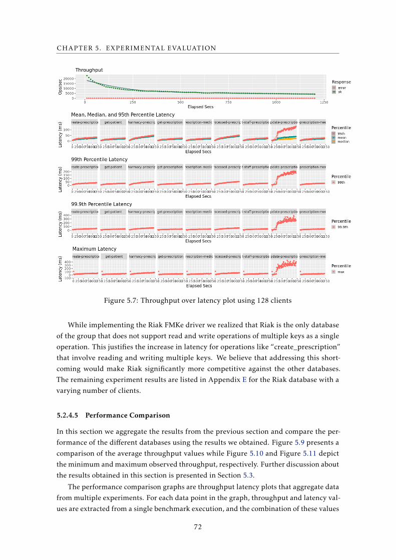
CHAPTER 5. EXPERIMENTAL EVALUATION
Figure 5.7: Throughput over latency plot using 128 clients
While implementing the Riak FMKe driver we realized that Riak is the only database
of the group that does not support read and write operations of multiple keys as a single
operation. This justifies the increase in latency for operations like “create_prescription”
that involve reading and writing multiple keys. We believe that addressing this short-
coming would make Riak significantly more competitive against the other databases.
The remaining experiment results are listed in Appendix E for the Riak database with a
varying number of clients.
5.2.4.5 Performance Comparison
In this section we aggregate the results from the previous section and compare the per-
formance of the different databases using the results we obtained. Figure 5.9 presents a
comparison of the average throughput values while Figure 5.10 and Figure 5.11 depict
the minimum and maximum observed throughput, respectively. Further discussion about
the results obtained in this section is presented in Section 5.3.
The performance comparison graphs are throughput latency plots that aggregate data
from multiple experiments. For each data point in the graph, throughput and latency val-
ues are extracted from a single benchmark execution, and the combination of these values
72

5.2. COMPARATIVE PERFORMANCE STUDY
Figure 5.8: Throughput over latency plot using 64 clients
becomes a single point in the plot. For increasing number of clients, we repeat the process
in order to determine the point at which a system has reached peak throughput. This can
be seen in the graphs as a latency spike that can also cause reduction in throughput. The
benchmark clients experience increased latency on their requests if they are generating
more load than the application server or database nodes can handle at once. This results
in requests becoming queued instead of instantly processed, leading to a bigger response
time. Throughput latency graphs are a good option to compare throughput and latency
between different systems at the same time, which otherwise would imply a graph to
compare each of the performance metrics.
The average throughput latency plot in Figure 5.9 indicates that AntidoteDB was
able to sustain a higher average throughput. Redis Cluster and Cassandra, while both
promising in terms of starting throughput, quickly decreased over time to a lower average
than AntidoteDB as seen from Figure 5.7 and Figure 5.6. Interestingly, the difference
between the average throughput in Cassandra and Redis Cluster seems negligible, despite
visibly behind AntidoteDB’s throughput.
Figure 5.10 shows the minimum observed throughput for each test case, which the-
oretically might be closer to the throughput stabilization point. There is a noticeable
73

CHAPTER 5. EXPERIMENTAL EVALUATION
Figure 5.9: Average throughput for all FMKe drivers
Figure 5.10: Minimum observed throughput over average latency
74

5.3. DISCUSSION
rise in Riak from last place to second, while still considerably distant from AntidoteDB.
Redis Cluster and Cassandra again have very similar results, but their sharp decrease in
throughput over time is clearly visible in this graph.
Figure 5.11: Maximum observed throughput over average latency
Finally, Figure 5.11 shows the maximum observed throughput during the workload
generation phase of the benchmark. Unlike the average throughput graph, Redis Cluster
takes the lead with a comfortable margin between it and AntidoteDB and Cassandra,
which now have very similar results. Riak, now last in the placements, reaches its peak
throughput at 8.000 operations per second and curiously is able to sustain it, unlike the
other databases, which suffer throughput losses at higher numbers of concurrent clients.
5.3 Discussion
Orchestrating and executing these experiments is very time consuming. There are several
steps that can be automated through the use of shell scripts, but these tend to be some-
what tightly coupled with the cloud platform on which the tests are being performed.
Hardware associated with instance types in the cloud may be upgraded at several points
in time, thus it is best to run the experiments within a small time window in order to min-
imize hardware heterogeneity. We understand that Riak looks unfavorable compared to
our other test subjects due to its lack of support for fetching and updating multiple keys at
once. Due to the replication strategies that each database uses, we are confident that Riak
would perform comparatively better in larger cluster deployments against Redis Cluster,
but we did not get the chance to explore this test case. Selecting more than 50-60 nodes,
past the limits of Riak Core, we would expect Cassandra to be the only viable option from
our set of storage systems. With regards to Antidote’s multiple data-center experiments,
there are other aspects to geo-replicated distributed databases, like the amount of time
75

CHAPTER 5. EXPERIMENTAL EVALUATION
that it takes for operations on one data-center to be propagated to others (data staleness),
that were not measured in these experiments.
Our decision to generate load for a 20 minute period allowed us to see how database
performance would evolve in a real scenario and that affected our average results in
Section 5.2.4.5. Any particular selection (minimum, maximum, or average throughput)
will favor different distributed data stores, so we present all results acknowledging that
there is an argument to be made for each one of the values:
• Minimum: we have presented the results and seen that in all experiments through-
put decreases slightly over time. Since we let the workload generator run for 20
minutes, an argument can be made that the last throughput values (i.e. the lowest)
are closer to the stabilization point of the storage system’s throughput and thus are
closer to the real performance limits of the database.
• Maximum: like we previously stated, the throughput decrease is not noticeable in
a time frame below 5 minutes, which would lead to apparently stable throughput
readings. Had we run the workload duration for a short period of time, our end
results would match what we see as the maximum (typically observed in the first
moments of generating load on the database).
• Average: Our workload generation process push the database systems to operate at
their peak capacity. Real deployments of these databases would take much longer
to reach the stabilization point since they would not be subject to such an intense
workload, making the expected throughput somewhere between the maximum and
the minimum observed.
There are counter-arguments for opting for any of the throughput values in detriment
of the others, but taking into consideration that we did not explore the performance limits
of these databases exhaustively, we feel that opting for the minimum or average would
not properly represent the potential of each database system. Selecting the maximum
throughput also seems to be in line with previous publications on comparative database
evaluation [42] [28]. This effectively makes Redis Cluster the best performing distributed
database within a single data-center.
5.4 Summary
We conducted two different experimental evaluations focusing on measuring different
aspects of database scalability and performance. From our results we were able to verify
that AntidoteDB’s performance scales approximately linearly with an increasing number
of data-centers. In the comparative test results, we obtained results that can be inter-
preted in different ways. The distributed database with the highest maximum throughput
was Redis Cluster, while AntidoteDB maintained the highest average throughput of the
76

5.4. SUMMARY
systems under test. In the following chapter we make some closing remarks regarding
the contributions of this work as well as some insights we gained from the experimen-
tal results. Finally, we end with a brief discussion on future work related to this thesis
concerning experimental scenarios we wish to explore.
77


Chapter
6Conclusions and Future Work
6.1 Conclusions
In this work we presented our proposal for a novel benchmark for distributed key-value
stores that is based on a real application in production in Denmark. We designed the inter-
face to allow both easy to implement, generic drivers, as well as more intricate drivers that
implement the full interface of the system being consistently more efficient. We presented
several data models that fit different data storage systems, and we included an equivalent
relational model alternative. This relational model variant will allow future performance
studies to be compared with our ongoing implementation of a relational ODBC database
driver for FMKe. This study will in turn objectively point out the performance difference
there is between relational and NoSQL databases, despite the differences in features and
consistency guarantees.
We have also detailed our implementation that we have made available in public code
repositories, which supports AntidoteDB, Redis, Riak and Cassandra. We demonstrated
how the FMKe application server can be configured to run with the different supported
storage systems and how to first populate the database with fictitious medical records and
then generate load on the application server using the Lasp Bench workload generator.
A significant effort went into making FMKe components simple to use, since we are
presenting it as a new standard for performance measurements in distributed databases.
With our experiments we were able to demonstrate the scalability of AntidoteDB on
several levels. Not only did its performance increase with the number of nodes in the
cluster, throughput also increased when multiple data-centers were added. In the compar-
ative experiments within a single data-center, we pointed out the performance between
AntidoteDB and Riak, and how Redis, running only in-memory, was able to reach higher
performance values. These experimental results not only compare the performance of the
79

CHAPTER 6. CONCLUSIONS AND FUTURE WORK
storage systems between themselves but also validate our implementation as an adequate
tool to conduct performance measurements from distributed databases.
We must note that the experiments presented in Chapter 5 were performed with a
limited budget in Amazon Web Services, and thus do not demonstrate the performance
of all databases in different scenarios. There are multiple configurations that were not
explored (e.g. using only in-memory storage), but this is not a limitation of our imple-
mentation. Designing experiments such that they are fair to all storage systems involved
in the comparison is not a trivial task. Any inefficiency in the FMKe driver, client li-
brary, and all other system components can be enough to invalidate the results for a given
database. For these reasons, we believe that the most important contribution of this work
is the benchmark implementation itself. We are convinced that the benchmark along
with its documentation will allow other developers to explore additional configurations
according to their requirements.
6.2 Future Work
As future work and to complement our single data-center study, we plan on implementing
an ODBC driver that would allow interaction with traditional relational databases. We
hope to observe the limits of distributed SQL databases and compare them with our
NoSQL database results. We would also like to extend our comparative performance
study to include larger deployments that demonstrate the scalability in terms of cluster
size. Finally, it would make sense to complete this comparative performance study by also
performing experiments in a geo-replicated environment and measure other properties
unrelated to performance, such as data consistency guarantees, data staleness and fault
tolerance.
80

Bibliography
[1] A NoSQL TPC-W benchmark with a Cassandra interface - GitHub. https://github.
com/PedroGomes/TPCw-benchmark. Accessed: 2017-07-10.
[2] P. S. Almeida, A. Shoker, and C. Baquero. “Delta state replicated data types.” In:
Journal of Parallel and Distributed Computing 111 (2018), pp. 162–173.
[3] S. Almeida, J. Leitão, and L. Rodrigues. “ChainReaction: a causal+ consistent
datastore based on chain replication.” In: Proceedings of the 8th ACM EuropeanConference on Computer Systems. ACM. 2013, pp. 85–98.
[4] Almeida, P.S., Shoker, A., Baquero, C.: Efficient state-based crdts by delta-mutation.CoRR abs/1410.2803 (2014). https://arxiv.org/pdf/1410.2803.pdf. Accessed:
2018-09-23.
[5] Amazon Web Services - Elastic Compute Cloud. http://aws.amazon.com/ec2/.
Accessed: 2018-12-03.
[6] AntidoteDB: A planet scale, highly available, transactional database - Website. https:
//www.antidotedb.eu. Accessed: 2018-12-16.
[7] Apache Cassandra - The Cassandra Query Language (CQL). http://cassandra.
apache.org/doc/latest/cql. Accessed: 2017-07-09.
[8] Apache Cassandra - Webpage. http://cassandra.apache.org. Accessed: 2017-12-
03.
[9] Apache Cassandra - Website. https://cassandra.apache.org. Accessed: 2018-12-
16.
[10] Apache CouchDB. https://couchdb.apache.org. Accessed: 2017-07-10.
[11] AWS re:Invent 2017: A Story of Netflix and AB Testing in the User Interface using Dy-namoDB - YouTube. https://www.youtube.com/watch?v=k8PTetgYzLA. Accessed:
2018-12-16.
[12] P. Bailis and K. Kingsbury. “The Network is Reliable.” In: Commun. ACM 57.9
(Sept. 2014), pp. 48–55. issn: 0001-0782. doi: 10.1145/2643130. url: http:
//doi.acm.org/10.1145/2643130.
[13] H. Berenson, P. Bernstein, J. Gray, J. Melton, E. O’Neil, and P. O’Neil. “A critique
of ANSI SQL isolation levels.” In: ACM SIGMOD Record. Vol. 24. 2. ACM. 1995,
pp. 1–10.
81

BIBLIOGRAPHY
[14] Booking.development Blog - Using Riak as Events Storage (Part 1 of 4). https://
medium.com/booking- com- development/using- riak- as- events- storage-
part-1-9b423f0ef97a. Accessed: 2018-12-16.
[15] E. Brewer. Spanner, TrueTime and the CAP Theorem. Tech. rep. 2017.
[16] CockroachDB - Mapping Table Data to Key-Value Storage. https://www.cockroachlabs.
com/blog/sql-in-cockroachdb-mapping-table-data-to-key-value-storage.
Accessed: 2017-07-09.
[17] Codd, E. F. “A Relational Model of Data for Large Shared Data Banks.” In: Commun.ACM 13.6 (June 1970), pp. 377–387. issn: 0001-0782. doi: 10.1145/362384.
362685. url: http://doi.acm.org/10.1145/362384.362685.
[18] B. F. Cooper, R. Ramakrishnan, U. Srivastava, A. Silberstein, P. Bohannon, H.-A.
Jacobsen, N. Puz, D. Weaver, and R. Yerneni. “PNUTS: Yahoo!’s hosted data serving
platform.” In: Proceedings of the VLDB Endowment 1.2 (2008), pp. 1277–1288.
[19] B. F. Cooper, A. Silberstein, E. Tam, R. Ramakrishnan, and R. Sears. “Benchmarking
cloud serving systems with YCSB.” In: Proceedings of the 1st ACM symposium onCloud computing. ACM. 2010, pp. 143–154.
[20] G. DeCandia, D. Hastorun, M. Jampani, G. Kakulapati, A. Lakshman, A. Pilchin, S.
Sivasubramanian, P. Vosshall, and W. Vogels. “Dynamo: amazon’s highly available
key-value store.” In: ACM SIGOPS operating systems review 41.6 (2007), pp. 205–
220.
[21] Discord Blog - How Discord Stores Billions of Messages. https://blog.discordapp.com/how-discord-stores-billions-of-messages-7fa6ec7ee4c7. Accessed:
2018-12-16.
[22] R. Elmasri and S. Navathe. Fundamentals of database systems. Addison-Wesley
Publishing Company, 2010.
[23] FMKe Application Server, GitHub Repository. https://github.com/goncalotomas/
FMKe. Accessed: 2018-09-22.
[24] FMKe Demonstration Screencast, January 2017 - YouTube. https://www.youtube.
com/watch?v=vsh5xtYPx5o. Accessed: 2018-09-21.
[25] FMKe Population Tool, GitHub Repository. https://github.com/goncalotomas/
fmke_populator. Accessed: 2018-09-22.
[26] P. Fouto, J. Leit ao, and N. Preguiça. “Practical and Fast Causal Consistent Partial
Geo-Replication.” In: 2018 IEEE 17th International Symposium on Network Comput-ing and Applications (NCA). IEEE. 2018, pp. 1–10.
[27] FSYNC(2) manual - Linux Programmer’s Manual. http://man7.org/linux/man-pages/man2/fdatasync.2.html. Accessed: 2018-12-03.
82

BIBLIOGRAPHY
[28] R. Gallersdörfer and M. Nicola. Improving performance in replicated databases throughrelaxed coherency. RWTH, Fachgruppe Informatik, 1995.
[29] Geo-Distributed Active-Active Conflict-free Replicated Redis Databases CRDB - Re-dis Enterprise Software. https : / / docs . redislabs . com / latest / rs / #geo -
distributed-active-active-conflict-free-replicated-redis-databases-
crdb. Accessed: 2018-12-16.
[30] S. Gilbert and N. Lynch. “Brewer’s conjecture and the feasibility of consistent,
available, partition-tolerant web services.” In: Acm Sigact News 33.2 (2002), pp. 51–
59.
[31] J. Gray. Database and Transaction Processing Performance Handbook. 1993.
[32] Implementing a Real World Application in the Lasp Programming Language, GoogleSummer of Code 2017 Project Archive. https://summerofcode.withgoogle.com/
archive/2017/projects/4917747754467328/. Accessed: 2018-09-22.
[33] Lasp Bench Load Generation Tool, GitHub Repository. https://github.com/lasp-
lang/lasp-bench. Accessed: 2018-09-22.
[34] A. van der Linde, J. Leitão, and N. Preguiça. “∆-CRDTs: making δ-CRDTs delta-
based.” In: Proceedings of the 2nd Workshop on the Principles and Practice of Consis-tency for Distributed Data. ACM. 2016, p. 12.
[35] W. Lloyd, M. J. Freedman, M. Kaminsky, and D. G. Andersen. “Don’t settle for
eventual: scalable causal consistency for wide-area storage with COPS.” In: Pro-ceedings of the Twenty-Third ACM Symposium on Operating Systems Principles. ACM.
2011, pp. 401–416.
[36] Marc Shapiro, Nuno Preguiça, Carlos Baquero, Marek Zawirski. Conflict-free ReplicatedData Types. [Research Report] RR-7687, 2011, pp.18. <inria-00609399v1>. https:
//hal.inria.fr/inria-00609399v1/document. Accessed: 2018-09-24.
[37] Moniz, Henrique and Leitão, João and Dias, Ricardo J and Gehrke, Johannes and
Preguiça, Nuno and Rodrigues, Rodrigo. “Blotter: Low latency transactions for
geo-replicated storage.” In: Proceedings of the 26th International Conference on WorldWide Web. International World Wide Web Conferences Steering Committee. 2017,
pp. 263–272.
[38] MySQL Replication Manual - MySQL Documentation. https://downloads.mysql.
com/docs/mysql-replication-excerpt-5.6-en.pdf. Accessed: 2018-12-16.
[39] NoSQL Key Value Database - Riak KV - Basho. http://basho.com/products/riak-
kv/. Accessed: 2017-07-10.
[40] S. Patil, M. Polte, K. Ren, W. Tantisiriroj, L. Xiao, J. López, G. Gibson, A. Fuchs,
and B. Rinaldi. “YCSB++: benchmarking and performance debugging advanced
features in scalable table stores.” In: Proceedings of the 2nd ACM Symposium onCloud Computing. ACM. 2011, p. 9.
83

BIBLIOGRAPHY
[41] Python-based framework of the TPC-C OLTP benchmark for NoSQL systems - GitHub.
https://github.com/apavlo/py-tpcc. Accessed: 2017-07-10.
[42] T. Rabl, S. Gómez-Villamor, M. Sadoghi, V. Muntés-Mulero, H.-A. Jacobsen, and S.
Mankovskii. “Solving big data challenges for enterprise application performance
management.” In: Proceedings of the VLDB Endowment 5.12 (2012), pp. 1724–1735.
[43] Redis Cluster Guide - Redis Labs. https://redis.io/topics/cluster-tutorial.
Accessed: 2018-12-03.
[44] Redis persistence demystified - antirez weblog. http://oldblog.antirez.com/post/
redis-persistence-demystified.html. Accessed: 2018-12-03.
[45] Redis Recommended Clients - redis.io. https://redis.io/clients. Accessed:
2018-12-07.
[46] Riak Core Documentation - GitHub Wiki. https://github.com/basho/riak_core/wiki. Accessed: 2018-12-16.
[47] Riak KV usage by industries - Basho. http://basho.com/industries/. Accessed:
2017-07-10.
[48] RUBiS Benchmark Documentation - OW2 Consortium Webpage. https://rubis.ow2.
org/doc/index.html. Accessed: 2018-12-16.
[49] A. Silberschatz, H. F. Korth, S. Sudarshan, et al. Database system concepts. Vol. 4.
McGraw-Hill New York, 1997.
[50] Smarter Coordinator Selection with Vnode Queue Soft Limits - Russell Brown Blog Poston GitHub. https://github.com/russelldb/riak_kv/blob/rdb/gh1661/docs/
soft-limit-vnode.md. Accessed: 2018-12-03.
[51] Stack Overflow Developer Survey 2018. https://insights.stackoverflow.com/
survey/2018/. Accessed: 2018-09-13.
[52] M. Stonebraker. “SQL Databases V. NoSQL Databases.” In: Commun. ACM 53.4
(Apr. 2010), pp. 10–11. issn: 0001-0782. doi: 10.1145/1721654.1721659. url:
http://doi.acm.org/10.1145/1721654.1721659.
[53] Transaction Processing Council - TPC C Benchmark Specification Document. http:
//www.tpc.org/tpc_documents_current_versions/pdf/tpc-c_v5.11.0.pdf.
Accessed: 2017-07-08.
[54] Transaction Processing Council - TPC H Benchmark Specification Document. http:
//www.tpc.org/tpc_documents_current_versions/pdf/tpc-h_v2.17.3.pdf.
Accessed: 2017-07-08.
[55] T. Warszawski and P. Bailis. “ACIDRain: Concurrency-Related Attacks on Database-
Backed Web Applications.” In: Proceedings of the 2017 ACM International Conferenceon Management of Data. SIGMOD ’17. Chicago, Illinois, USA: ACM, 2017, pp. 5–20.
isbn: 978-1-4503-4197-4. doi: 10.1145/3035918.3064037. url: http://doi.
acm.org/10.1145/3035918.3064037.
84

BIBLIOGRAPHY
[56] Who uses Redis - TechStacks. https://techstacks.io/tech/redis. Accessed:
2018-12-07.
[57] Why Your Riak Cluster Should Have At Least Five Nodes - Basho Technical Blog (2012-04-26). http : / / basho . com / posts / technical / why - your - riak - cluster -
should-have-at-least-five-nodes. Accessed: 2018-12-03.
85


Appendix
ACQL Table Creation Statements
The following CQL statements are required to build Cassandra tables compatible with
FMKe’s driver:
Listing A.1: Cassandra Table Creation Script
1 CREATE TABLE IF NOT EXISTS fmke.patients (
2 ID int PRIMARY KEY,
3 Name text,
4 Address text,
5 );
6
7 CREATE TABLE IF NOT EXISTS fmke.pharmacies (
8 ID int PRIMARY KEY,
9 Name text,
10 Address text,
11 );
12
13 CREATE TABLE IF NOT EXISTS fmke.medical_staff (
14 ID int PRIMARY KEY,
15 Name text,
16 Address text,
17 Speciality text,
18 );
19
20 CREATE TABLE IF NOT EXISTS fmke.treatment_facilities (
21 ID int PRIMARY KEY,
22 Name text,
23 Address text,
24 Type text,
25 );
26
27
87

APPENDIX A. CQL TABLE CREATION STATEMENTS
28 CREATE TABLE IF NOT EXISTS fmke.prescriptions (
29 ID int,
30 PatID int,
31 DocID int,
32 PharmID int,
33 DatePrescribed timestamp,
34 DateProcessed timestamp,
35 PRIMARY KEY (ID)
36 );
37
38 CREATE TABLE IF NOT EXISTS fmke.patient_prescriptions (
39 PatientID int,
40 PrescriptionID int,
41 PRIMARY KEY (PatientID, PrescriptionID)
42 );
43
44 CREATE TABLE IF NOT EXISTS fmke.pharmacy_prescriptions (
45 PharmacyID int,
46 PrescriptionID int,
47 PRIMARY KEY (PharmacyID, PrescriptionID)
48 );
49
50 CREATE TABLE IF NOT EXISTS fmke.staff_prescriptions (
51 StaffID int,
52 PrescriptionID int,
53 PRIMARY KEY (StaffID, PrescriptionID)
54 );
55
56 CREATE TABLE IF NOT EXISTS fmke.prescription_drugs (
57 PrescriptionID int,
58 Drug text,
59 PRIMARY KEY (PrescriptionID, Drug)
60 );
88

Appendix
BAntidoteDB Performance Results
This appendix contains individual test results for the AntidoteDB tests run in the com-
parative performance study.
89

APPENDIX B. ANTIDOTEDB PERFORMANCE RESULTS
B.1 32 Clients
Figure B.1: Throughput over latency plot using 32 clients
90

B.2. 64 CLIENTS
B.2 64 Clients
Figure B.2: Throughput over latency plot using 64 clients
91

APPENDIX B. ANTIDOTEDB PERFORMANCE RESULTS
B.3 128 Clients
Figure B.3: Throughput over latency plot using 128 clients
92

B.4. 256 CLIENTS
B.4 256 Clients
Figure B.4: Throughput over latency plot using 256 clients
93

APPENDIX B. ANTIDOTEDB PERFORMANCE RESULTS
B.5 512 Clients
Figure B.5: Throughput over latency plot using 512 clients
94

Appendix
CCassandra Performance Results
This appendix contains individual test results for the Cassandra tests run in the compar-
ative performance study.
95

APPENDIX C. CASSANDRA PERFORMANCE RESULTS
C.1 32 Clients
Figure C.1: Throughput over latency plot using 32 clients
96

C.2. 64 CLIENTS
C.2 64 Clients
Figure C.2: Throughput over latency plot using 64 clients
97

APPENDIX C. CASSANDRA PERFORMANCE RESULTS
C.3 128 Clients
Figure C.3: Throughput over latency plot using 128 clients
98

C.4. 256 CLIENTS
C.4 256 Clients
Figure C.4: Throughput over latency plot using 256 clients
99

APPENDIX C. CASSANDRA PERFORMANCE RESULTS
C.5 512 Clients
Figure C.5: Throughput over latency plot using 512 clients
100

Appendix
DRedis Cluster Performance Results
This appendix contains individual test results for the Redis Cluster tests run in the com-
parative performance study.
101

APPENDIX D. REDIS CLUSTER PERFORMANCE RESULTS
D.1 32 Clients
Figure D.1: Throughput over latency plot using 32 clients
102

D.2. 64 CLIENTS
D.2 64 Clients
Figure D.2: Throughput over latency plot using 64 clients
103

APPENDIX D. REDIS CLUSTER PERFORMANCE RESULTS
D.3 128 Clients
Figure D.3: Throughput over latency plot using 128 clients
104

D.4. 256 CLIENTS
D.4 256 Clients
Figure D.4: Throughput over latency plot using 256 clients
105

APPENDIX D. REDIS CLUSTER PERFORMANCE RESULTS
D.5 512 Clients
Figure D.5: Throughput over latency plot using 512 clients
106

Appendix
ERiak Performance Results
This appendix contains individual test results for the Riak tests run in the comparative
performance study.
107

APPENDIX E. RIAK PERFORMANCE RESULTS
E.1 32 Clients
Figure E.1: Throughput over latency plot using 32 clients
108

E.2. 64 CLIENTS
E.2 64 Clients
Figure E.2: Throughput over latency plot using 64 clients
109

APPENDIX E. RIAK PERFORMANCE RESULTS
E.3 128 Clients
Figure E.3: Throughput over latency plot using 128 clients
110

E.4. 256 CLIENTS
E.4 256 Clients
Figure E.4: Throughput over latency plot using 256 clients
111

APPENDIX E. RIAK PERFORMANCE RESULTS
E.5 512 Clients
Figure E.5: Throughput over latency plot using 512 clients
112