Artificial Neural Networks for Compression of Gray Scale Images: A Benchmark
13
See discussions, stats, and author profiles for this publication at: http://www.researchgate.net/publication/264082353 Artificial Neural Networks for Compression of Gray Scale Images: A Benchmark CONFERENCE PAPER · OCTOBER 2013 DOI: 10.1007/978-3-642-33212-8_20 READS 15 3 AUTHORS, INCLUDING: Osvaldo De Souza Universidade Federal do Ceará 12 PUBLICATIONS 4 CITATIONS SEE PROFILE Paulo César Cortez Universidade Federal do Ceará 89 PUBLICATIONS 184 CITATIONS SEE PROFILE Available from: Osvaldo De Souza Retrieved on: 25 September 2015
Transcript of Artificial Neural Networks for Compression of Gray Scale Images: A Benchmark

Seediscussions,stats,andauthorprofilesforthispublicationat:http://www.researchgate.net/publication/264082353
ArtificialNeuralNetworksforCompressionofGrayScaleImages:ABenchmark
CONFERENCEPAPER·OCTOBER2013
DOI:10.1007/978-3-642-33212-8_20
READS
15
3AUTHORS,INCLUDING:
OsvaldoDeSouza
UniversidadeFederaldoCeará
12PUBLICATIONS4CITATIONS
SEEPROFILE
PauloCésarCortez
UniversidadeFederaldoCeará
89PUBLICATIONS184CITATIONS
SEEPROFILE
Availablefrom:OsvaldoDeSouza
Retrievedon:25September2015
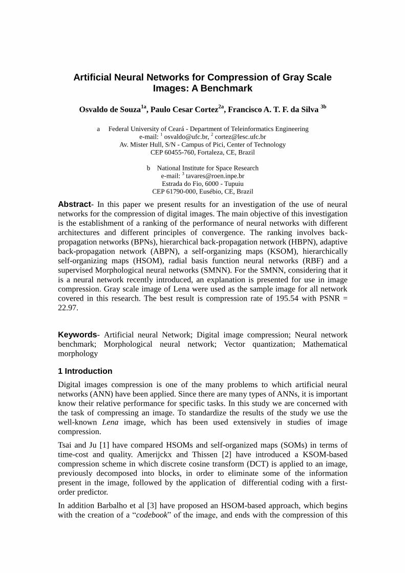
Artificial Neural Networks for Compression of Gray Scale Images: A Benchmark
Osvaldo de Souza
1a, Paulo Cesar Cortez
2a, Francisco A. T. F. da Silva
3b
a Federal University of Ceará - Department of Teleinformatics Engineering
e-mail: 1 [email protected],
Av. Mister Hull, S/N - Campus of Pici, Center of Technology
CEP 60455-760, Fortaleza, CE, Brazil
b National Institute for Space Research
e-mail: 3 [email protected]
Estrada do Fio, 6000 - Tupuiu
CEP 61790-000, Eusébio, CE, Brazil
Abstract- In this paper we present results for an investigation of the use of neural
networks for the compression of digital images. The main objective of this investigation
is the establishment of a ranking of the performance of neural networks with different
architectures and different principles of convergence. The ranking involves back-
propagation networks (BPNs), hierarchical back-propagation network (HBPN), adaptive
back-propagation network (ABPN), a self-organizing maps (KSOM), hierarchically
self-organizing maps (HSOM), radial basis function neural networks (RBF) and a
supervised Morphological neural networks (SMNN). For the SMNN, considering that it
is a neural network recently introduced, an explanation is presented for use in image compression. Gray scale image of Lena were used as the sample image for all network
covered in this research. The best result is compression rate of 195.54 with PSNR =
22.97.
Keywords- Artificial neural Network; Digital image compression; Neural network
benchmark; Morphological neural network; Vector quantization; Mathematical
morphology
1 Introduction
Digital images compression is one of the many problems to which artificial neural
networks (ANN) have been applied. Since there are many types of ANNs, it is important
know their relative performance for specific tasks. In this study we are concerned with
the task of compressing an image. To standardize the results of the study we use the
well-known Lena image, which has been used extensively in studies of image
compression.
Tsai and Ju [1] have compared HSOMs and self-organized maps (SOMs) in terms of
time-cost and quality. Amerijckx and Thissen [2] have introduced a KSOM-based
compression scheme in which discrete cosine transform (DCT) is applied to an image,
previously decomposed into blocks, in order to eliminate some of the information
present in the image, followed by the application of differential coding with a first-
order predictor.
In addition Barbalho et al [3] have proposed an HSOM-based approach, which begins
with the creation of a “codebook” of the image, and ends with the compression of this
codebook by Huffman’s algorithm. Given that most of the compression is performed by
Huffman’s algorithm, the performance of the approach depends on a complex process in
addition to the ANN's work.
In recent work, Vaddella and Rama [4] have presented and discussed results for various
Ann’s architectures for image compression, and in their considerations they presented
results for HSOM, KSOM, BPN, HBPN and ABPN.
Reddy et al [5] have presented and discussed results concerning RBF-based digital
image compression while Barbalho et al [3] have done the same for HSON-based
compression. Wang and Gou [6] have studied an approach that begins with the
decomposition of the image at different scales using a wavelet transform (WT) in order
to obtain an orthogonal wavelet representation of the image, continues with the
application for each scale of the discrete Karhumen-Loeve transform (KLT), and ends
with vector quantization by means of a self-development neural network. Thus Wang
and Gou’s approach is more a wavelet-based approach than an ANN-based approach to
image compression. It is clear from the literature that many types of ANNs have been
successfully applied to digital image compression over a period of many years. Despite
this, however, no work providing an extensive comparison of various ANNs for digital
image compression has been published. In this paper we, provide such a comparison,
including results for a supervised morphological neural network (SMNN) [7].
We choose Lena as the target image in order to make the best use of the results available
in the literature. So we focused our efforts on investigating the performance of SMNN.
The SMNN belongs to a class of neural networks whose theory is based on
mathematical morphology (MM). Banon and Barrera [8] have produced an extensive
work investigating all aspects of the MM, and this work has been complemented by
Banon [9]. In the next section, we present a brief review of the mathematical
formulation of SMNNs regarding their use in image compression.
2 Supervised Morphological Neural Network
In general, the processing at a node in a classical ANN is defined by the equation
𝑏𝑗 = 𝑓𝑗 (∑ 𝑎𝑖𝑤𝑗𝑖
𝑁
𝑖=1
), (1)
while the processing at a node in a SMNN, is defined by the equation
𝑦𝑘 = 𝛹𝑡 ∘ 𝜙. (2)
Thus, in the definition of a morphological neuron of the SMNN, the additive junction
and its arithmetical operations (multiplication and addition) inside the activation
function 𝑓𝑗(. ) in equation (1) are replaced in equation (2) by 𝛹𝑡 ∘ 𝜙 which is a
composed threshold operator. An understanding of the definition of 𝛹𝑡 and its
composition 𝛹𝑡 ∘ 𝜙 is provided in [10].
2.1 SMNN Gray Level Tolerance
In Banon [11] are given complete demonstrations and proofs of all morphological
operators in which the operator 𝛹𝑡 is based on. Banon and Faria [12] gave a brief
presentation of the same definitions, and Silva [10] extended some morphological
operators in order to compose 𝛹𝑡 ∘ 𝜙. In de Souza et al [7] are given details regarding
all SMNN’s architecture and equations, including online learning process and error
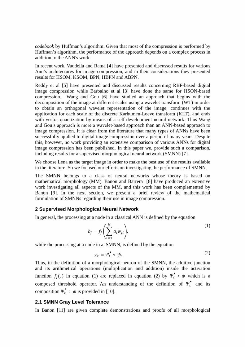
correction for morphological neurons with tolerances of gray level variations. Figure 1
illustrated this gray level tolerance.
Figure 1: Example of gray level tolerance in morphological approach for template
matching, adapted from Banon and Faria [12]
In figure 1 the values of 𝑐1 and 𝑐2 are calculated according to
𝑑𝜇 = 𝜇(𝑔) − 𝜇(𝑓) , 𝑐1 = 𝑑𝜇 − 𝐹
2 , 𝑐2 = 𝑑𝜇 +
𝐹
2 ,
(3)
where 𝜇(𝑔) and 𝜇(𝑓) are gray level average of image g and f , respectively. 𝐹 is the
length of the interval [𝑐1, 𝑐2], centered at 𝑑𝜇, and 𝑓𝑤− and 𝑓𝑤
+ are defined in Banon and
Faria [12].
Observing Figure 1 one can notice that a short tolerance interval may produce great
level of tolerance of variations; in that figure, for a sub-image [40 52 40] and 𝐹 = 4 the
SMNN accepts all of the following sequences:
Table 1: partial list of valid sequences for sub-image [40 52 40] and F=4.
[40 52 40] , [40 53 40], [40 55 40], [40 56 40],
[41 52 40] , [41 53 40], [41 55 40], [41 56 40],
[42 52 40] , [42 53 40], [42 55 40], [42 56 40],
[43 52 40] , [43 53 40], [43 55 40], [43 56 40],
[44 52 40] , [44 53 40], [44 55 40], [44 56 40],
[40 52 41] , [40 53 41], [40 55 41], [40 56 41],
[41 52 41 , [41 53 41], [41 55 41], [41 56 41],
[42 52 41] , [42 53 41], [42 55 41], [42 56 41],
[43 52 41] , [43 53 41], [43 55 41], [43 56 41],
[44 52 41] , [44 53 41], [44 55 41], [44 56 41],
[40 52 42] , [40 53 42], [40 55 42], [40 56 42],
[41 52 42 , [41 53 42], [41 55 42], [41 56 42],
[42 52 42] , [42 53 42], [42 55 42], [42 56 42],
[43 52 42] , [43 53 42], [43 55 42], [43 56 42],
[44 52 42] , [44 53 42], [44 55 42], [44 56 42].
Notice that Table 1 does not show all accepted sequences for F=4; a complete table
would contain up to 125 (= (5) ∗ (5) ∗ (5)) possibilities, since the acceptance range is
[40-44 52-56 40-44]. Suppose that sub-image [39 52 40] is under consideration for
compression by an SMNN, which already contains trained neurons for all 125
possibilities mentioned above. Since the range is [40- 44 52-56 40-44], the sub-image
[39 52 40] is out of range. However, the sub-image would match if we accept a
minimum of 2 hits per 3 pixels. Therefore, if we desired this level of quality, a threshold
𝑡 = 0.66 would be suitable. This is the role that the threshold 𝑡 plays in our approach.
2.2 SMNN Compression Process for a Gray Scale Image
During the compression, for each sub-image processed, the SMNN returns the number
of the neuron that compressed the sub-image. This number must be preserved for each
sub-image processed so that the compressed data can later be expanded to recover the
original image. According to de Souza et al [7] the SMNN requires the definition of two
important elements: (a) the level of tolerance for the matching condition, expressed by
the length of the 𝐹 interval; and (b) the level of the threshold 𝑡. The 𝐹 interval can be
understood as the SMNN constraint for variation of the pixel’s value. The compression
process starts with the splitting of the image into 𝑛 sub-images. Then, each sub-image is
compressed.
3 Computer Simulations and Discussion
In order to fill the aforementioned gap in the literature regarding the application of
morphological neural networks to digital image compression, we have conducted an
investigation based on the paradigms presented in the previous section. All experiments
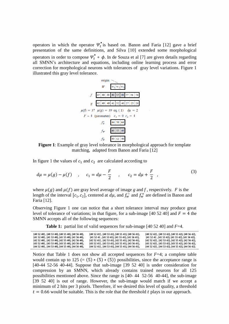
reported in this paper use the Lena picture as the standard image sample. Lena is a well-
known, freely available image that has been used in many studies concerning digital
image processing.
Figure 2 A gray scale Lena image
3.1 Detailed Results for SMNN-based Compression
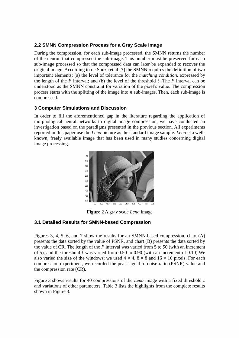
Figures 3, 4, 5, 6, and 7 show the results for an SMNN-based compression, chart (A)
presents the data sorted by the value of PSNR, and chart (B) presents the data sorted by
the value of CR. The length of the 𝐹 interval was varied from 5 to 50 (with an increment
of 5), and the threshold 𝑡 was varied from 0.50 to 0.90 (with an increment of 0.10).We
also varied the size of the windows; we used 4 × 4, 8 × 8 and 16 × 16 pixels. For each
compression experiment, we recorded the peak signal-to-noise ratio (PSNR) value and
the compression rate (CR).
Figure 3 shows results for 40 compressions of the Lena image with a fixed threshold 𝑡
and variations of other parameters. Table 3 lists the highlights from the complete results
shown in Figure 3.
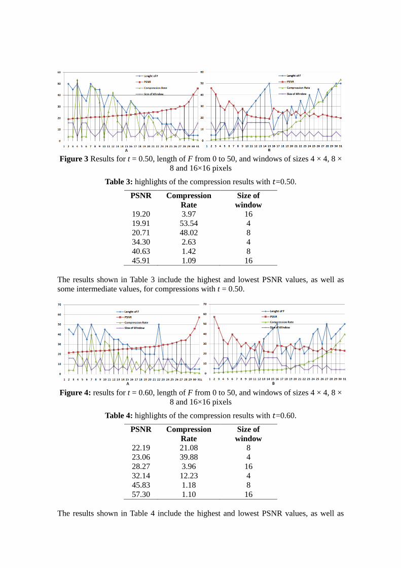
Figure 3 Results for t = 0.50, length of F from 0 to 50, and windows of sizes 4 × 4, 8 ×
8 and 16×16 pixels
Table 3: highlights of the compression results with 𝑡=0.50.
PSNR Compression
Rate
Size of
window
19.20 3.97 16
19.91 53.54 4
20.71 48.02 8
34.30 2.63 4
40.63 1.42 8
45.91 1.09 16
The results shown in Table 3 include the highest and lowest PSNR values, as well as
some intermediate values, for compressions with t = 0.50.
Figure 4: results for t = 0.60, length of F from 0 to 50, and windows of sizes 4 × 4, 8 ×
8 and 16×16 pixels
Table 4: highlights of the compression results with 𝑡=0.60.
PSNR Compression
Rate
Size of
window
22.19 21.08 8
23.06 39.88 4
28.27 3.96 16
32.14 12.23 4
45.83 1.18 8
57.30 1.10 16
The results shown in Table 4 include the highest and lowest PSNR values, as well as
some intermediate values, for compressions with t = 0.60.
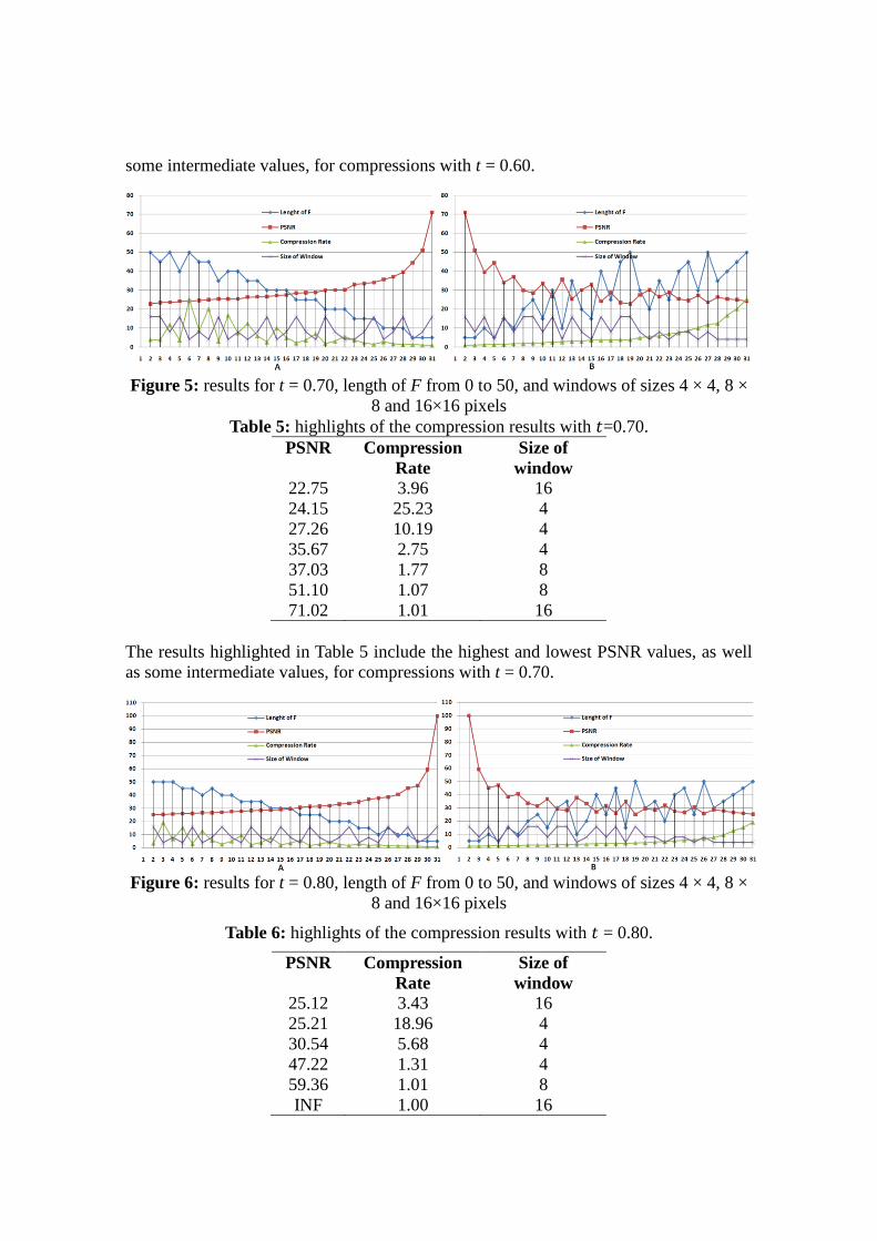
Figure 5: results for t = 0.70, length of F from 0 to 50, and windows of sizes 4 × 4, 8 ×
8 and 16×16 pixels
Table 5: highlights of the compression results with 𝑡=0.70.
PSNR Compression
Rate
Size of
window
22.75 3.96 16
24.15 25.23 4
27.26 10.19 4
35.67 2.75 4
37.03 1.77 8
51.10 1.07 8
71.02 1.01 16
The results highlighted in Table 5 include the highest and lowest PSNR values, as well
as some intermediate values, for compressions with t = 0.70.
Figure 6: results for t = 0.80, length of F from 0 to 50, and windows of sizes 4 × 4, 8 ×
8 and 16×16 pixels
Table 6: highlights of the compression results with 𝑡 = 0.80.
PSNR Compression
Rate
Size of
window
25.12 3.43 16
25.21 18.96 4
30.54 5.68 4
47.22 1.31 4
59.36 1.01 8
INF 1.00 16
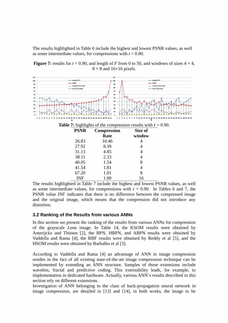
The results highlighted in Table 6 include the highest and lowest PSNR values, as well
as some intermediate values, for compressions with t = 0.80.
Figure 7: results for t = 0.90, and length of F from 0 to 50, and windows of sizes 4 × 4,
8 × 8 and 16×16 pixels.
Table 7: highlights of the compression results with 𝑡 = 0.90.
PSNR Compression
Rate
Size of
window
26.83 10.46 4
27.92 8.39 4
31.13 4.85 4
38.11 2.33 4
40.05 1.54 8
41.54 1.81 4
67.20 1.01 8
INF 1.00 16
The results highlighted in Table 7 include the highest and lowest PSNR values, as well
as some intermediate values, for compressions with t = 0.90. In Tables 6 and 7, the
PSNR value INF indicates that there is no difference between the compressed image
and the original image, which means that the compression did not introduce any
distortion.
3.2 Ranking of the Results from various ANNs
In this section we present the ranking of the results from various ANNs for compression
of the grayscale Lena image. In Table 14, the KSOM results were obtained by
Amerijckx and Thissen [2], the BPN, HBPN, and ABPN results were obtained by
Vaddella and Rama [4], the RBF results were obtained by Reddy et al [5], and the
HSOM results were obtained by Barbalho et al [3].
According to Vaddella and Rama [4] an advantage of ANN in image compression
resides in the fact of all existing state-of-the-art image compression technique can be
implemented by extending an ANN structure. Samples of those extensions include
wavelets, fractal and predictive coding. This extensibility leads, for example, to
implementation in dedicated hardware. Actually, various ANN´s results described in this
section rely on different extensions.
Investigation of ANN belonging to the class of back-propagation neural network in
image compression, are detailed in [13] and [14], in both works, the image to be
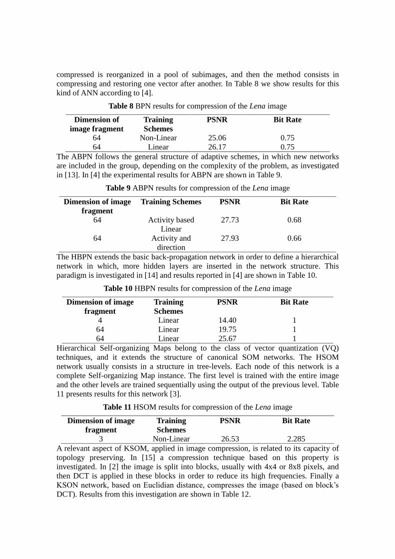
compressed is reorganized in a pool of subimages, and then the method consists in
compressing and restoring one vector after another. In Table 8 we show results for this
kind of ANN according to [4].
Table 8 BPN results for compression of the Lena image
Dimension of
image fragment
Training
Schemes
PSNR Bit Rate
64 Non-Linear 25.06 0.75
64 Linear 26.17 0.75
The ABPN follows the general structure of adaptive schemes, in which new networks
are included in the group, depending on the complexity of the problem, as investigated
in [13]. In [4] the experimental results for ABPN are shown in Table 9.
Table 9 ABPN results for compression of the Lena image
Dimension of image
fragment
Training Schemes PSNR Bit Rate
64 Activity based
Linear
27.73 0.68
64 Activity and
direction
27.93 0.66
The HBPN extends the basic back-propagation network in order to define a hierarchical
network in which, more hidden layers are inserted in the network structure. This
paradigm is investigated in [14] and results reported in [4] are shown in Table 10.
Table 10 HBPN results for compression of the Lena image
Dimension of image
fragment
Training
Schemes
PSNR Bit Rate
4 Linear 14.40 1
64 Linear 19.75 1
64 Linear 25.67 1
Hierarchical Self-organizing Maps belong to the class of vector quantization (VQ)
techniques, and it extends the structure of canonical SOM networks. The HSOM
network usually consists in a structure in tree-levels. Each node of this network is a
complete Self-organizing Map instance. The first level is trained with the entire image
and the other levels are trained sequentially using the output of the previous level. Table
11 presents results for this network [3].
Table 11 HSOM results for compression of the Lena image
Dimension of image
fragment
Training
Schemes
PSNR Bit Rate
3 Non-Linear 26.53 2.285
A relevant aspect of KSOM, applied in image compression, is related to its capacity of
topology preserving. In [15] a compression technique based on this property is
investigated. In [2] the image is split into blocks, usually with 4x4 or 8x8 pixels, and
then DCT is applied in these blocks in order to reduce its high frequencies. Finally a
KSON network, based on Euclidian distance, compresses the image (based on block’s
DCT). Results from this investigation are shown in Table 12.
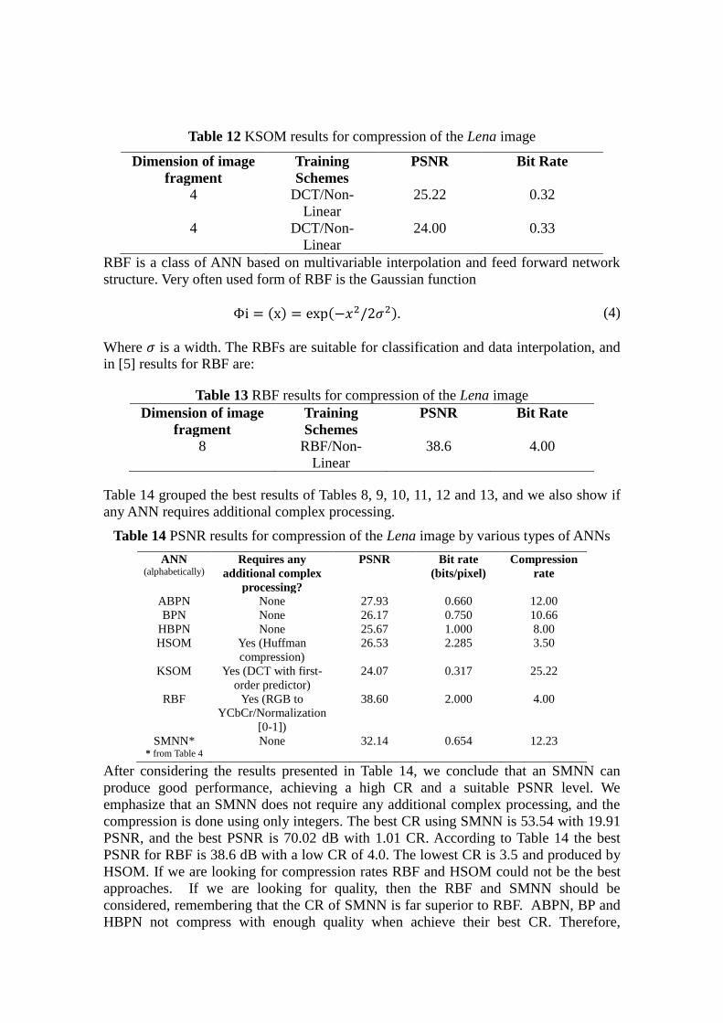
Table 12 KSOM results for compression of the Lena image
Dimension of image
fragment
Training
Schemes
PSNR Bit Rate
4 DCT/Non-
Linear
25.22 0.32
4 DCT/Non-
Linear
24.00 0.33
RBF is a class of ANN based on multivariable interpolation and feed forward network
structure. Very often used form of RBF is the Gaussian function
Φi = (x) = exp(−𝑥2/2𝜎2). (4)
Where 𝜎 is a width. The RBFs are suitable for classification and data interpolation, and
in [5] results for RBF are:
Table 13 RBF results for compression of the Lena image
Dimension of image
fragment
Training
Schemes
PSNR Bit Rate
8 RBF/Non-
Linear
38.6 4.00
Table 14 grouped the best results of Tables 8, 9, 10, 11, 12 and 13, and we also show if
any ANN requires additional complex processing.
Table 14 PSNR results for compression of the Lena image by various types of ANNs
ANN (alphabetically)
Requires any
additional complex
processing?
PSNR Bit rate
(bits/pixel)
Compression
rate
ABPN None 27.93 0.660 12.00
BPN None 26.17 0.750 10.66
HBPN None 25.67 1.000 8.00
HSOM Yes (Huffman
compression)
26.53 2.285 3.50
KSOM Yes (DCT with first-
order predictor)
24.07 0.317 25.22
RBF Yes (RGB to
YCbCr/Normalization
[0-1])
38.60 2.000 4.00
SMNN* None 32.14 0.654 12.23 * from Table 4
After considering the results presented in Table 14, we conclude that an SMNN can
produce good performance, achieving a high CR and a suitable PSNR level. We
emphasize that an SMNN does not require any additional complex processing, and the
compression is done using only integers. The best CR using SMNN is 53.54 with 19.91
PSNR, and the best PSNR is 70.02 dB with 1.01 CR. According to Table 14 the best
PSNR for RBF is 38.6 dB with a low CR of 4.0. The lowest CR is 3.5 and produced by
HSOM. If we are looking for compression rates RBF and HSOM could not be the best
approaches. If we are looking for quality, then the RBF and SMNN should be
considered, remembering that the CR of SMNN is far superior to RBF. ABPN, BP and
HBPN not compress with enough quality when achieve their best CR. Therefore,
according to the analysis of data from multiple Tables and in especial the Table 14, the
SMNN appears to be the best choice for image compression among the ANNs
considered in this investigation. Extending the evaluation of SMNN, we also would like
to highlight that, as can be seen in Tables 3, 4, 5, 6, and 7, the best PSNR results, as well
as good compression rates, were obtained with windows of 4 × 4 pixels. For this reason,
we decided to investigate the interval from 1 to 70 for F, with a fixed threshold t = 0.80
and a window of 4 × 4 pixels. We present some considerations about this investigation
in the next section.
3.2 An Open Issue
There is an open issue regarding the performance of an SMNN: How to deal with
(downsize) the indices for the windows? Most vector quantization (VQ) compression
approaches deal with the problem of managing a large number of pieces resulting from
subdivision of the original image. These pieces commonly called “codewords” are
grouped in a “codebook”. The problem is that we need to know how to rebuild the
compressed image, so we need to keep a mapping between each codeword and the
region of the image we can rebuild with it. For the purposes of comparison, the sub-
images resulting from the splitting of the image are a type of codeword. Since the Lena
image has 512×512 pixels, if we use a window with a size of, say, 2×2 pixels, we would
have 65536 windows to process and maintain a mapping for. This means that 65,536
bytes at least are used for mapping, at least of 25% of compression is wasted, and the
processing time is increased. We have already reported a compression of the Lena
image with a value of CR=163.84 obtained with 2×2 window size; but a simulation of
this compression required about 11 h of processing time. In this particular simulation,
we used a simple variable run-length (VRE) coding strategy in which a long sequence
of the same symbol (where a “long” sequence has a length greater than 3) is replaced by
a shorter sequence while the data related with the 65536 window’s indices is saved to
the disk. Since in our approach, and in the results presented in the previous section, we
did not use any kind of compression in storing the mapping, the performance of an
SMNN could be increased through the application of a technique for reducing the
amount of space required to store the mapping. Hu et al [16] have proposed an
improved image coding schema, in which, to reduce the cost of storing compressed
codes, they use a two-stage lossless coding approach based on linear prediction and
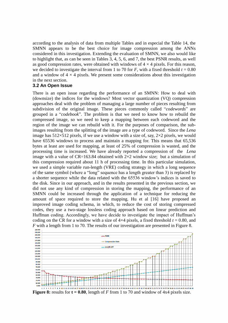
Huffman coding. Accordingly, we have decide to investigate the impact of Huffman’s
coding on the CR for a window with a size of 4×4 pixels, a fixed threshold t = 0.80, and
F with a length from 1 to 70. The results of our investigation are presented in Figure 8.
Figure 8: results for t = 0.80, length of F from 1 to 70 and window of 4x4 pixels size.
By using Huffman’s coding, we can compress the map of windows, and we can achieve
a highest compression rate of CR = 195.542 with PSNR = 22.971, and a lowest
compression rate of CR = 5.734 with PSNR = 56.482. As can be seen from Figure 8,
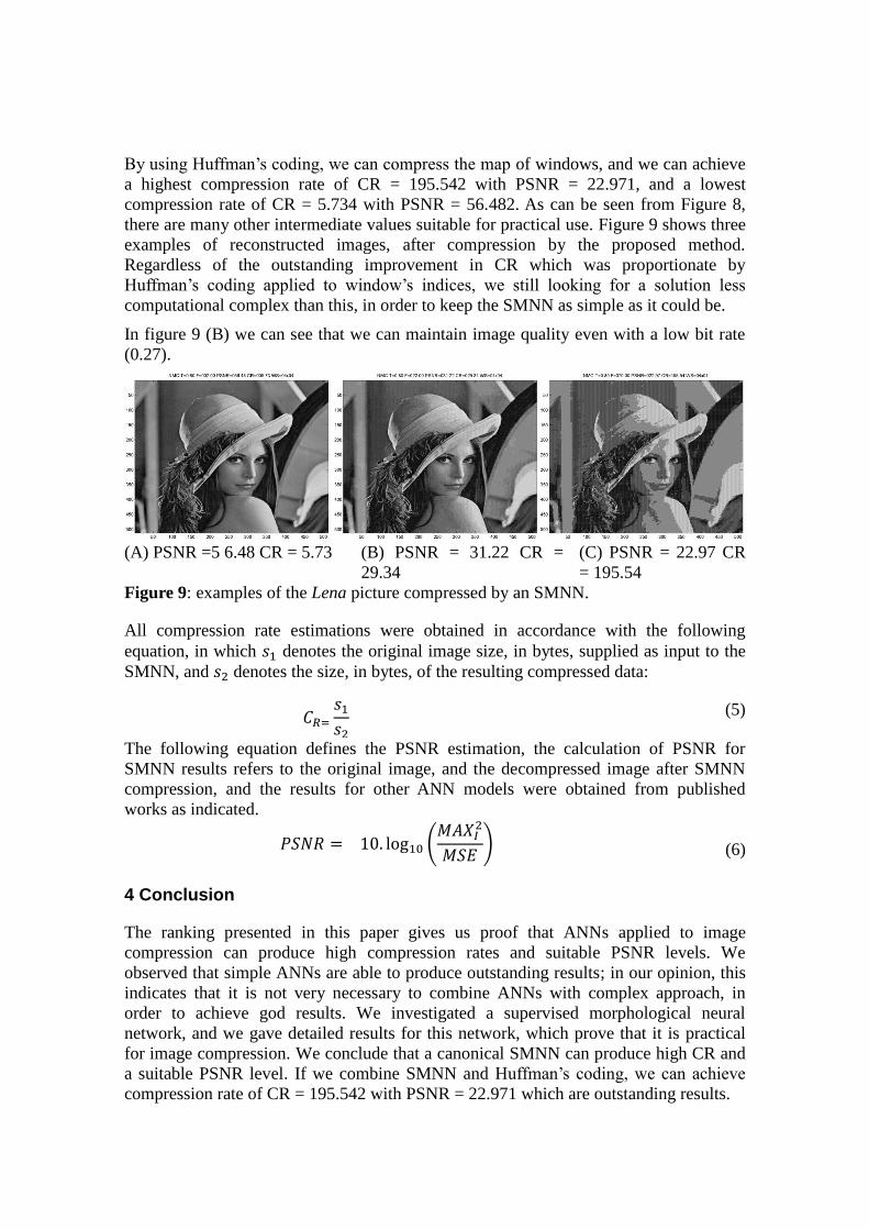
there are many other intermediate values suitable for practical use. Figure 9 shows three
examples of reconstructed images, after compression by the proposed method.
Regardless of the outstanding improvement in CR which was proportionate by
Huffman’s coding applied to window’s indices, we still looking for a solution less
computational complex than this, in order to keep the SMNN as simple as it could be.
In figure 9 (B) we can see that we can maintain image quality even with a low bit rate
(0.27).
(A) PSNR =5 6.48 CR = 5.73 (B) PSNR = 31.22 CR =
29.34
(C) PSNR = 22.97 CR
= 195.54
Figure 9: examples of the Lena picture compressed by an SMNN.
All compression rate estimations were obtained in accordance with the following
equation, in which 𝑠1 denotes the original image size, in bytes, supplied as input to the
SMNN, and 𝑠2 denotes the size, in bytes, of the resulting compressed data:
𝐶𝑅=
𝑠1
𝑠2 (5)
The following equation defines the PSNR estimation, the calculation of PSNR for
SMNN results refers to the original image, and the decompressed image after SMNN
compression, and the results for other ANN models were obtained from published
works as indicated.
𝑃𝑆𝑁𝑅 = 10. log10 (𝑀𝐴𝑋𝐼
2
𝑀𝑆𝐸)
(6)
4 Conclusion
The ranking presented in this paper gives us proof that ANNs applied to image
compression can produce high compression rates and suitable PSNR levels. We
observed that simple ANNs are able to produce outstanding results; in our opinion, this
indicates that it is not very necessary to combine ANNs with complex approach, in
order to achieve god results. We investigated a supervised morphological neural
network, and we gave detailed results for this network, which prove that it is practical
for image compression. We conclude that a canonical SMNN can produce high CR and
a suitable PSNR level. If we combine SMNN and Huffman’s coding, we can achieve
compression rate of CR = 195.542 with PSNR = 22.971 which are outstanding results.
References
1. Tsay, C., Ju, J.H., 2009. ELSA: A new image compression using an expanding-leaf
segmentation algorithm. LNAI 5579, 624–633.
2. Amerijckx, C., Thissen, P., 1988. Image compression by self-organized Kohonen
map. IEEE Transaction on Neural Networks 9(3).
3. Barbalho, J.M., Costa, J.A.F., Neto, A.D.D., Netto, M.L.A., 2003. Hierarchical and
dynamic SOM applied to image compression. Proceedings of the International Joint
Conference on Neural Networks 1, 753–758.
4. Vaddella, R.P.V., Rama, K., 2010. Artificial neural networks for compression of
digital images: A review. International Journal of Reviews in Computing, v3, 75–82.
5. Reddy, et al., 2012. Image compression and reconstruction using a new approach by
artificial neural network. International Journal of Image Processing 6(2), 68–85.
6. Wang, J.H., Gou, K.J., 1988. Image compression using wavelet transform and self-
development neural network. IEEE International Conference on Systems, Man and
Cybernetics 4, 4104–4108.
7. de Souza, O., Cortez, P. C., Silva, F. A.T.F., 2012. Grayscale Images and RGB Video:
Compression by Morphological Neural Network. In 5th
Workshop on Artificial Neural
Networks in Pattern Recognition. LNCS vol 7477. pp. 213-224
8. Banon, G.J.F., Barrera J., 1993. Decomposition of mappings between complete
lattices by mathematical morphology – part I: general lattices. Signal Processing 30(3),
299–327.
9. Banon, G.J.F., 1995. Characterization of translation invariant elementary
morphological operators between gray-level images. INPE, São José dos Campos, SP,
Brazil.
10. Silva, F. A. T. F., 1999, Rede Morfológica Não Supervisionada., Proceedings of the
IV Brazilian Conference on neural Networks. 400-405.
11. Banon, G. J. F., 1995a, Characterization of translation invariant elementary
morphological operators between gray-level images. INPE, São José dos Campos, SP,
propositions 1.2 and 1.3, p 7.
12. Banon, G.J.F., Faria, S.D., 1997. Morphological approach for template matching.
Brazilian Symposium on Computer Graphics and Image Processing Proceedings, IEEE
Computer Society.
13. R.D. Dony, S. Haykin, “Neural network approaches to image compression”, Proc.
IEEE, Vol. 83, No. 2, Feb. 1995, pp 288-303
14. A. Namphol, S. Chin, M. Arozullah, “Image compression with a hierarchical neural
network”, IEEE Trans. Aerospace Electronic Systems, Vol 32, No.1, January 1996, pp
326-337
15. E. A. Riskin, L. E. Atlas, and S. R. Lay, “Ordered neural maps and their applications
to data compression,” in Neural Networks for Signal Processing ’91, IEEE Wkshp., pp.
543–551.
16. Hu, Y.-C., et al., 2012. Improved vector quantization scheme for grayscale image
compression. Opto-Electronics Review 20(2), 187–193.