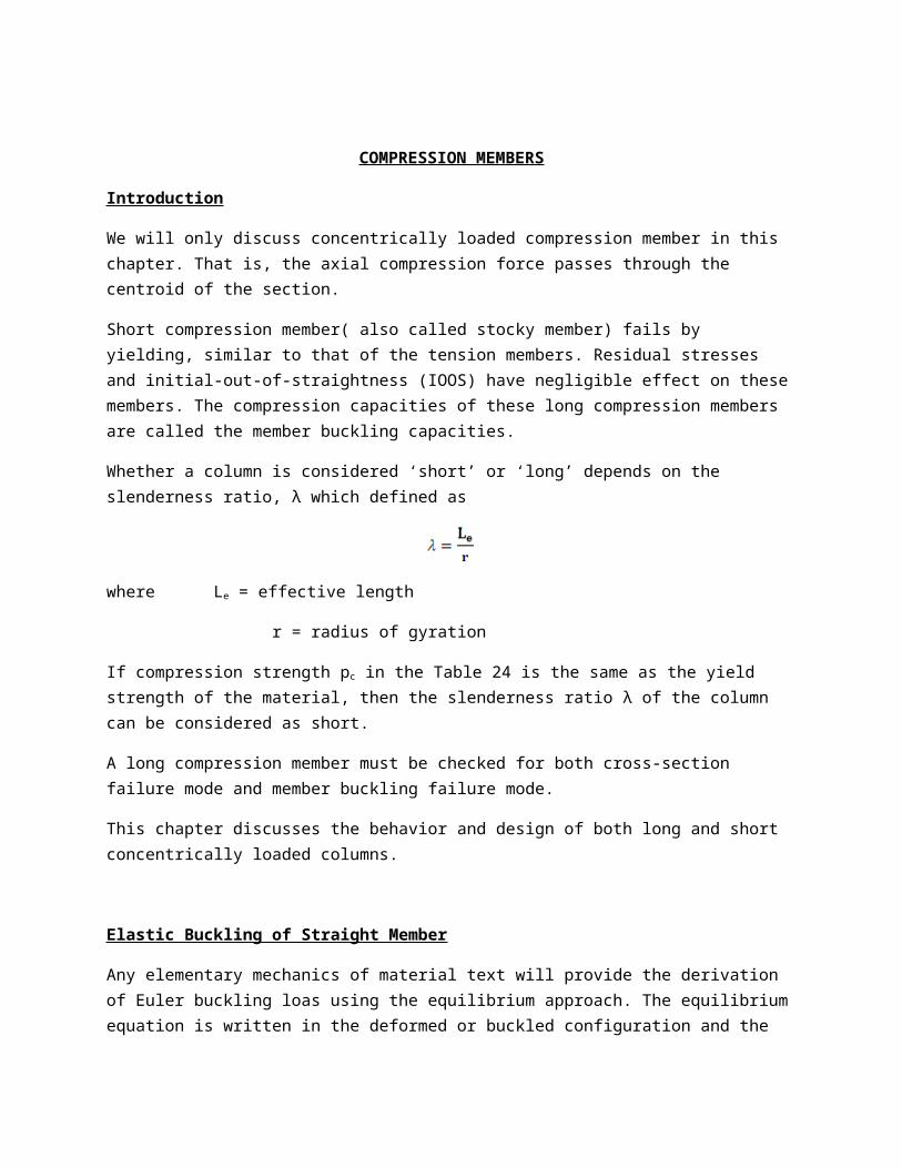
COMPRESSION MEMBERS

Introduction

We will only discuss concentrically loaded compression member in this chapter. That is, the axial compression force passes through the centroid of the section.

Short compression member( also called stocky member) fails by yielding, similar to that of the tension members. Residual stresses and initial-out-of-straightness (IOOS) have negligible effect on thesemembers. The compression capacities of these long compression members are called the member buckling capacities.

Whether a column is considered ‘short’ or ‘long’ depends on the slenderness ratio, λ which defined as

where Le = effective length

r = radius of gyration

If compression strength pc in the Table 24 is the same as the yield strength of the material, then the slenderness ratio λ of the column can be considered as short.

A long compression member must be checked for both cross-section failure mode and member buckling failure mode.

This chapter discusses the behavior and design of both long and short concentrically loaded columns.

Elastic Buckling of Straight Member

Any elementary mechanics of material text will provide the derivation of Euler buckling loas using the equilibrium approach. The equilibriumequation is written in the deformed or buckled configuration and the

L-δ

L

Yδ

P

A

resulting differential equation is solve at the Euler buckling load PE given by

The derivation of the above equation using energy method is shown below.

There are significant difference between the theoretical and actual behavior, especially for slenderness ratio between 0.2 and 1.6, largely due to two factors which are not considered in Euler’s derivation.

a. Residual stressesb. Initial out of straightness (IOOS)

Design equation must account for the difference between the real behavior and the theoretical formulation.

Effect of Residual Stresses

Real column has residual stresses. The causes part of the column to reach yield stress at stress level below the yield stress. The net result is that the Young’s Modulus E is not constant, but become non-linear when the partial yielding occurs. This effect is called inelastic buckling.

See notes on elastic buckling (Shanley Model)

Hence, the buckling curves for column with residual stresses accordingto the Shenley is given by

X

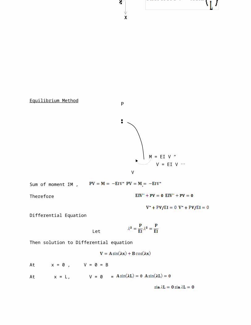
Equilibrium Method

Sum of moment ƩM ,

Therefore

Differential Equation

Let

Then solution to Differential equation

At x = 0 , V = 0 = B

At x = L, V = 0 =

Ѵ = EI V ,,,

≠ 0V

P

P

M = EI V “

Since

Therefore

Energy Method

Work done,

Strain Energy

Energy difference,

Le = 0.5Lor K=0.5

Le = 2.0Lor K=2.0

L

Le = 0.7Lor K=0.7

L L

Diffrentiate wrt A,

Therefore

Other Boundary Conditions

Different type of boundary condition can be accounted for by using theeffective length factor ‘K’

i.e PcrPcr Pcr

Pcr

P

M = PV0

Pcr

Vt = V + V0

A

A0

In all cases,

Beams with initial Imperfection

4 + dx

U1 U2

Curvature

2

= 2

2

Energy Difference, π = U1 + U2 – W

π 4

2 2

Differentiate

4 - 2

2

2

where

Since Vt = V + V0

Pcr

OR

Thus, the second-order effect caused by axial load can be estimated bymagnifying the effect of first order using magnification factor

Magnification Factor

The Perry-Robertson Approach (Annex C)

Consider a column with IOOS, δo. Upon application of load, P, the totaldeflection δ will be (recap: see notes on elastic buckling):

The maximum stress, pmax is given by

Where,

S = Section Modulus

A = Cross-sectional area

So, we can write

Where,

I = Moment of Inertia

c = Distance from Neutral Axis to the maximum fiber

r = Radius of gyration

The maximum stress can be rewritten as

η

Let

and assume that failure occurs when pmax = py

then

OR

Which can be written as the quadratic equation;

Rearranging

Alternatively, from Eqn PR 1, we can write

Solving the quadratic equation leads to,

Where

Instead of using Eqn. PR 3, the BS5950 further rearrange this equationby completing the square

-----------

-----------

-----------

OR

The design strength for the column is given by

Where,

Ag = Gross area

γM1 = 1.0 (Partial material safety factor)

In the above derivation, η is the dimensionless imperfection parameteror the Perry Factor. In BS5950, the Perry Factor is rewritten as

Where

λ = Slenderness ratio.

a = Robertson constant (1925)

Thus Eqn. PR 4 is called the Perry-Robertson curve. It is a convenientrepresentation of the column buckling capacity. The values of Robersonconstant, a is obtained from calibration exercise with the existing test results and are given by:

a = 2.0 for column curve a

a = 3.5 for column curve b

a = 5.5 for column curve c

-----------

a = 8.0 for column curve d

Where curve a,b,c and d refer to the various buckling curve in Table 24

By adjusting the value of λ0 ratio, the buckling curve can adjust for the plateau below which the column is considered as a short (or stockycolumn) and do not undergo buckling. In BS5950, the slenderness ratio λ is defines as

Accordingly, the Euler buckling stress is given by

It can be seen from Figure PR 1 (Pc/py vs λ=LE/r) that at a slenderness parameter λc of 0.2, the column buckling curve is practically reaches the squash load Py. In the figure λc is the more generally accepted definition of slenderness parameter given by

Substitute, λc = 0.2 when λ0 = LE/r

OR

The buckling curves can be schematically shown as

-----------

Figure PR 1

Note: Even though the original Perry-Roberson curve was derived assuming initial out of straightness only and no residual stresses, the calibration exercise with test results means that the Robertson constant actually account for BOTH initial imperfection and residual stresses.

The different buckling curves a,b,c and d account for the different types of members, different buckling axis, different thickness and etcas defined in Table 23 (BS5950). We can note the following trend for UC Table 23.

1. Thinner member (≤ 40 mm) has a more favorable buckling curve compared to the thicker member. This is due to the larger imperfection and more residual stresses in the thickness member.

2. Buckling about x-x axis has a more favorable buckling curve compared to the buckling about the y-y axis. This is because the tip of the UC flanges has compression residual stresses (see earlier lectures on steel material) which ad unfavorably to the flexural buckling compression stresses.

Effective Length Factors (Table 22)

NON-SWAY MODE SWAY MODE

END B Positio Positio Positio Positio None Directi Partial

nn

Direction

nDirecti

on

nPartial on

END A Position

Position

Position

Direction

Position

Partial

Position

Direction

Position

Direction

Position

Direction

Theory 1.0 0.7 0.5 2.0 1.0Table22 1.0 0.85 0.7 0.85 2.0 1.2 1.5

At x = L y = - δ

At x = L,

KL

L

PE

Y

---------

2-Span Column- 1-Span Load Elastically Restrained Column

Column A-B buckles elastically but restrained by column B-C

X δ

PE

α1

δ

E2I2

E1I1

C

B

A

K1L1Δ1

α1

X1

Y1

L1

L2 θ

BB

PE

Buckling Curve

At X1= L1 , Y1 = -δ

Therefore,

But , therefore

Also,

Therefore,

Moment at B,

and

Substitute Eqn. PR 6 and

From Eqn. PR 7

-----------

-----------

Solve for K1 and

in principle, we can solve for K1 using Eqn. PR 8 and therefore obtain the buckling load Pcr

Example:

Use 200 x 200 x 16 SHS Grade 275

I1 = I2 = 6524 x104 mm4

E1 = E2 =205000 N/mm2

L2= 12m

L1= 6m

-----------

Held in position, Partial Restraint in direction

E1 , I1

Held in

E2 , I2

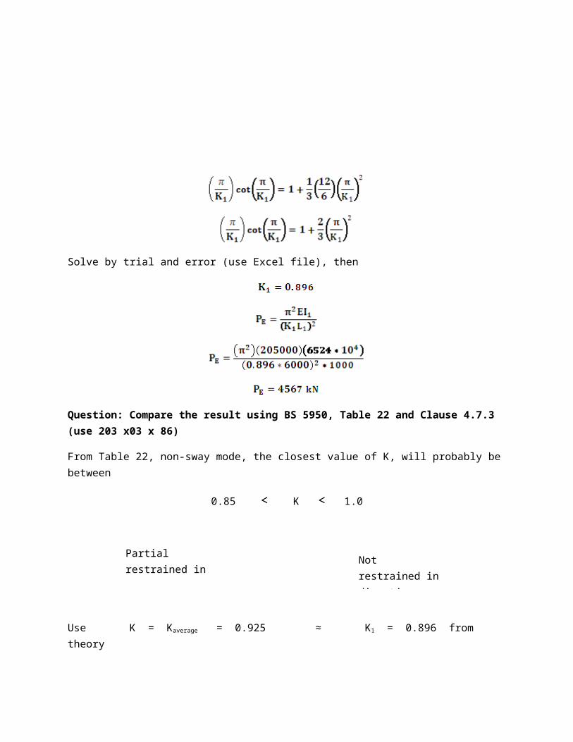
Solve by trial and error (use Excel file), then

Question: Compare the result using BS 5950, Table 22 and Clause 4.7.3 (use 203 x03 x 86)

From Table 22, non-sway mode, the closest value of K, will probably bebetween

0.85 < K < 1.0

Use K = Kaverage = 0.925 ≈ K1 = 0.896 from theory

Partial restrained in direction

Not restrained indirection

NOTE: For non-sway column it is always safe to use K = 1.0

(about 6% lower thantheory)

if we use K = 1.0

PE = 3666 kN (about 20% lower than theory)

Having PE value now we can proceed to determine Pc

From Table 23, SHS (Cold Formed) is curve C

Therefore α = 5.5 (Clause C.2)

For the theoretical curve, K = K1 = 0.896

OR

Therefore,

Therefore,

The easier way is by applying Table 24 (c)

λ = 71.872 ≈ 72

py = 275 N/mm2

pc = 177 N/mm2 ( Refer Table 24(c))

We proceed with the other K value using Table 24 (c)

Same as before

Refer [Eqn. PR

Refer [Eqn. PR

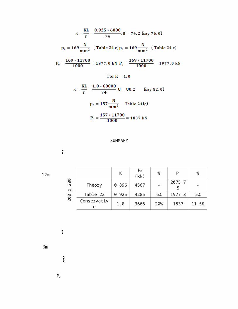
SUMMARY

Pc

200 x

200

x 16 S

HS

6m

12m K PE

(kN) % Pc %

Theory 0.896 4567 - 2075.75 -

Table 22 0.925 4285 6% 1977.3 5%Conservativ

e 1.0 3666 20% 1837 11.5%

E

D

Flexural stiffness Continuity needed

Continuity in Flexural Stiffness broken

Column Splice using Full-contact bearing Connection

This type of connection is able to transmit full axial force. However,the continuity in flexural stiffness is broken.

Typically, the connection is at every 3 floors. Experience has shown that it is safe to use K=1.0 for all columns.

However, do not place this connection on the first or the last floor. Column must maintain flexural continuity in the first and the last floor.

Flexural stiffness Continuity needed

Flexural stiffness Continuity needed

A

B

C

Elastic Brace Requirement

What values of brace stiffness, β such that

Clearly, if β = 0

Thus, as β increases, the elastic buckling load increases from

β = 0 β = ‘Full Brace’

Consider a column with IOOS = Δ0. When it buckles, the deflection will increase by a amount Δ.

L

L

PE

β

Low Brace

Full Brace

PE

β

PE

Partial Brace

let βreq be the required stiffness so that

For a column that buckles in 2 sine-waves as shown above, a hinge isformed at mid-span

Sum of moment (ƩM),

PE

βreq

L

L

F/2

F/2

F

Δ

Δ0

Hinge

PE

Foe ideal column, Δ0 = 0

Therefore

The required strength in the brace is

OR

If

Thus, we cannot have braced stiffness equal to the ideal brace stiffness. Even for small value of IOOS = Δ0, the brace force become too large.

Consider the case when

Then, brace force

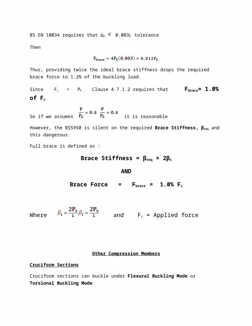
BS EN 10034 requires that Δ0 < 0.003L toleranceThen

Thus, providing twice the ideal brace stiffness drops the required brace force to 1.2% of the buckling load.

Since Fc < PE , Clause 4.7.1.2 requires that Fbrace= 1.0% of Fc

So if we assumes it is reasonable

However, the BS5950 is silent on the required Brace Stiffness, βreq and this dangerous.

Full brace is defined as :

Brace Stiffness = βreq = 2βi

AND

Brace Force = Fbrace = 1.0% Fc

Where and Fc = Applied force

Other Compression Members

Cruciform Sections

Cruciform sections can buckle under Flexural Buckling Mode or Torsional Buckling Mode

Flexural Buckling Mode

Where

Torsional Buckling Mode

Where,

H = Warping Constant

LE = Effective length under torsional buckling

J = Torsional constant =

where IP = Polar Moment of Inertia

For Cruciform section, Warping constant, H is small and can beneglected

t

t

b

b

b

b

Therefore,

Substitute

It can be seen that torsional buckling of cruciform section is similarto local buckling of outstand flange. The local buckling capacity is,

Y

X

LE

t=6mm

t=6mm

b=100mmb=100mm

b=100mmb=100mm

Where K = 0.425 for Outstand Flange

Example

The cruciform section shown below has thickness of 6mm and length 3000mm

a) Determine the torsional buckling loadb) Determine the flexural buckling loadc) If effective length , LE = 3000mm, which mode control the

buckling Take ν = 0.3

Buckling Stress

Area

a) To calculate column buckling load

Method 1 (Torsional Buckling)

Method 2 (Local Buckling)

b) To calculate flexural buckling

c) From the calculations, local buckling load controls, PE=680.35 kN

Equal Angle Sections (EA)

Equal angle have different moment of inertia

Ixx = Iyy (Geometric Axis)

Iuu (Maximum Principle Axis)

Ivv (Minimum Principle axis)

( Refer Moment and product of inertia)

Centroid

Shear Centre

y

y

xx

v

v

u

u

v

v

If the resultant shear forces during buckling passes through the ShearCentre and is parallel to the principle axis, no twisting will occur. This will be the case for a centrally load Equal angle (EA), where buckling will occur on the minimum principle axis

Flexural

v

(Centrally Loaded EA)

v

v

v

Flexural- Torsional

y

y

x

y

x x

Due to eccentricities in loading, non-symmetrical boundary condition (such as bolting on 0ne leg only). The flexural-torsional buckling modes cannot be ignored. Moreover, different connection details will lead to different stiffness at the end and hence different effective length factors.

BS 5950 accounts for all these factors by checking for buckling in 3-axix, namely: v-v axis, a-a axis and b-b axis (Table 25 and Clause 4.7.10 and Clause 4.7.10.2)

For Equal Angle (EA), the a-a and b-b axis are the same

In summary, EA fails by one of two buckling modes

a) Flexural buckling about the minimum v-v axisb) Combine twisting and bending about x-x (or y-y) axis (Flexural-

torsional)

Clause 4.7.10.2 provides the slenderness ratio appropriate for these buckling modes. Also shown summarized in Table 25

These slenderness ratios are largely empirical. These compressive stress can then be etermind using Table 24.

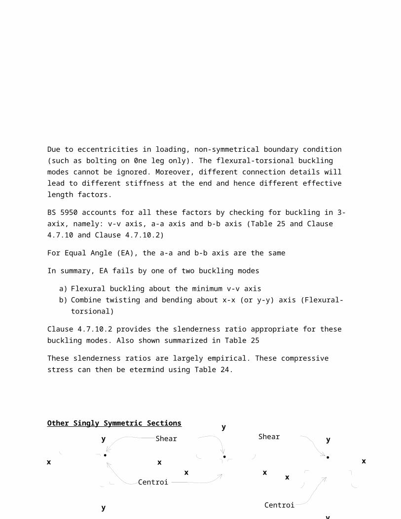
Other Singly Symmetric Sections

y

x x

y

x

Centroid

Shear Shear

Centroid

Similar to the case of Equal Angle, these sections will also buckle intwo possible modes

a) Flexural buckling about the minimum axis.b) Combine twisting and bending about the strong axis. (Flexural

Torsional Mode)

Clause 4.7.10.3 through 4.7.10.5 provides slenderness ratios for thesesections.

Example:

Determine the compression strength of the Tee section column shownbelow. The column is 1500 mm long (effective length) and connected byfour (4) bolts to the flange.

C.G = 46.45 mm rx = 61.39 mm

A = 5928 mm2 ry = 67.52 mm

Ix = 2.2343 x 107 mm4 Steel grade, S275

t=12

t=12

150150

20046.45

y

x xC.G

y

Iy = 2.7028 x 107 mm4

Table 25, Clause 4.7.10.5(a) (4 bolts)

47.1

use λx = 47.1 ----------------Control