Linear and non-linear features of the Taylor–Green dynamo

C. R. Physique 9 (2008) 749–756

http://france.elsevier.com/direct/COMREN/

The dynamo effect/L’effet dynamo

Linear and non-linear features of the Taylor–Green dynamo

Yannick Ponty a,∗, Pablo D. Mininni b,d, Jean-Philipe Laval c, Alexandros Alexakis a,d,Julien Baerenzung a,d, François Daviaud e, Bérengère Dubrulle e, Jean-François Pinton f,

Héléne Politano a, Annick Pouquet d

a Observatoire de la Côte d’Azur, CNRS and Université de Nice Sophia-Antipolis, BP 4229, Nice cedex 04, Franceb Departamento de Física, Facultad de Ciencias Exactas y Naturales, Universidad de Buenos Aires, Ciudad Universitaria,

1428 Buenos Aires, Argentinac Laboratoire de mécanique de Lille, CNRS, boulevard Paul-Langevin, 59655 Villeneuve d’Asq, France

d NCAR, P.O. Box 3000, Boulder, Colorado 80307-3000, USAe Service de physique de l’état condensé, CNRS et CEA-Saclay, 91191 Gif-sur-Yvette, France

f Laboratoire de physique, de l’École normale supérieure de Lyon, CNRS et Université de Lyon, 46, allée d’Italie, 69007 Lyon, France

Available online 6 September 2008

Abstract

The Taylor–Green flow is a model flow sharing many properties with the von Kármán flow, in which experimental turbulentdynamo action has recently been achieved. We present here recent numerical results on the Taylor–Green dynamo instability, bothin the linear and non-linear regime. Various properties are considered, such as the influence of turbulence, the energy transferbetween different scales, the spatial structure of the neutral mode, the nature of the bifurcation and the saturation mechanisms. Wealso discuss the role of the velocity fluctuations on the dynamo onset. To cite this article: Y. Ponty et al., C. R. Physique 9 (2008).© 2008 Académie des sciences. Published by Elsevier Masson SAS. All rights reserved.

Résumé

Étude linéaire et non linéaire d’une dynamo produite par un forçage de Taylor–Green. Un écoulement turbulent forçé parun tourbillon de type Taylor–Green, partage de nombreuses propriétés avec l’écoulement de von Kármán dans lequel une dynamoturbulente a été récemment mise en évidence expérimentalement. Nous présentons des résultats récents de dynamos numériquesengendrées par des tourbillons de Taylor–Green dans les régimes linéaire et non linéaire. Nous discutons certaines de ses propriétéscomme l’influence de la turbulence, le transfert d’énergie entre différentes échelles, la structure du mode neutre, la nature de labifurcation et les mécanismes de saturation. Nous discutons également le rôle joué par les fluctuations de vitesse sur le seuil de ladynamo. Pour citer cet article : Y. Ponty et al., C. R. Physique 9 (2008).© 2008 Académie des sciences. Published by Elsevier Masson SAS. All rights reserved.

Keywords: Dynamo; Magnetohydrodynamics; Turbulence; Taylor–Green

Mots-clés : Dynamo ; Magnétohydrodynamique ; Turbulence ; Taylor–Green

* Corresponding author.E-mail address: [email protected] (Y. Ponty).

1631-0705/$ – see front matter © 2008 Académie des sciences. Published by Elsevier Masson SAS. All rights reserved.doi:10.1016/j.crhy.2008.07.007

750 Y. Ponty et al. / C. R. Physique 9 (2008) 749–756

1. Introduction

Dynamo action, the self generation of magnetic field by a conducting moving fluid, is considered to be the mainsource of magnetic fields in the universe [1]. Over the past decades, experimental efforts have been devoted to theunderstanding of this magnetic induction [2–7] and dynamo action. To date, three groups have successfully achieveddynamos in liquid sodium laboratory experiments [8–11].

In parallel, several groups have been studying the problem using numerical methods. Ideally, one should buildrealistic simulations of the dynamos (natural or laboratory) taking into account the precise geometry, the effect ofthe fluid and magnetic boundary conditions. This is currently achieved using finite element, finite volume or finitedifference mesh schemes [12–14]. However, it is possible to study numerically some aspects of experimental dynamobehaviour with simple three-dimensional periodic boundary conditions. We review here several numerical resultsobtained using the Taylor–Green forcing in a periodic box.

2. Numerical method

Incompressible turbulent flows have been intensively studied in a periodic space, a classical mathematical frame-work for theories [15] as well as for numerical simulations of isotropic and homogeneous turbulence [16,17]. In thisgeometry, the pseudo-spectral numerical method is the most precise global numerical method for a fixed mesh size. Inthe present work, we use the pseudo-spectral method initiated by the work of Orszag and Patterson (1971) [16]. Thesuccess of this method is essentially due to the high accuracy and the efficiency of the Fast Fourier Transform.

2.1. Basic equations

We consider the incompressible magnetohydrodynamic equations (1), (2)

∂v∂t

+ v · ∇v = −∇P + j × B + ν∇2v + F (1)

∂B∂t

+ v · ∇B = B · ∇v + η∇2B (2)

together with ∇ · v = ∇ · B = 0; a constant mass density ρ = 1 is assumed. Here, v stands for the velocity field,B the magnetic field (in units of Alfvén velocity), j = (∇ × B)/μ0 the current density, ν the kinematic viscosity, η themagnetic diffusivity and P is the pressure. The forcing term F is the Taylor–Green vortex (TG) [18],

FTG(k0) = F0

[ sin(k0x) cos(k0y) cos(k0z)

−cos(k0x) sin(k0y) cos(k0z)

0

](3)

As direct numerical simulations (DNS) are rapidly limited, different sub-grid models have been used in order toreach the highest possible kinetic Reynolds numbers: (i) Large Eddy Simulation (LES) for the hydrodynamic field[19] with no model in the induction equation [20,21]; (ii) modelling of the full MHD system with a filtering, using the‘alpha model’ [22,23]; and (iii) using a dynamical spectral LES scheme [24,25].

2.2. Non-dimensional numbers

In our code, the dimensional form of the MHD (1), (2) equations is computed, and dimensionless numbers arecalculated a posteriori, using the numerical output. We define the Reynolds numbers as Rv = LV

νand Rm = LV

ηwith

a characteristic velocity V , length scale L and the viscosity ν or the magnetic diffusivity η. There are several possiblechoices for these characteristic quantities. For the velocity, one may use the root mean square (r.m.s), the average intime or the maximum of the velocity field. Similarly, for the length scale one may use the size of the box, the integralscale of the fluid or the Taylor micro-scale. In the studies reported here, several different choices have been made andwe will give the corresponding definitions in each particular case.

Y. Ponty et al. / C. R. Physique 9 (2008) 749–756 751

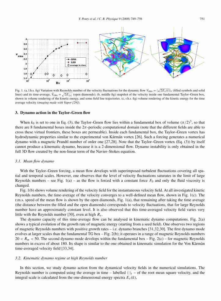
Fig. 1. (a, l.h.s. fig) Variation with Reynolds number of the velocity fluctuations for the dynamic flow Vrms = 〈√2Ev(t)〉t (filled symbols and solidlines) and its time-average, V̄rms = √

2E〈v〉 (open diamonds); (b, middle fig) snapshot of the velocity inside one fundamental Taylor–Green box,shown in volume rendering of the kinetic energy, and some field line trajectories. (c, r.h.s. fig) volume rendering of the kinetic energy for the timeaverage velocity (imaging made with Vapor [29]).

3. Dynamo action in the Taylor–Green flow

When k0 is set to one in Eq. (3), the Taylor–Green flow lies within a fundamental box of volume (π/2)3, so thatthere are 8 fundamental boxes inside the 2π -periodic computational domain (note that the different fields are able tocross these virtual frontiers, these boxes are permeable). Inside each fundamental box, the Taylor–Green vortex hashydrodynamic properties similar to the experimental von Kármán vortex [26]. Such a forcing generates a numericaldynamo with a magnetic Prandtl number of order one [27,28]. Note that the Taylor–Green vortex (Eq. (3)) by itselfcannot produce a kinematic dynamo, because it is a 2-dimensional flow. Dynamo instability is only obtained in thefull 3D flow created by the non-linear term of the Navier–Stokes equation.

3.1. Mean flow dynamo

With the Taylor–Green forcing, a mean flow develops with superimposed turbulent fluctuations covering all spa-tial and temporal scales. However, one observes that the level of velocity fluctuations saturates in the limit of largeReynolds numbers – see Fig. 1(a) – as the flow is forced with a constant force F0 and only the fluid viscosity ischanged.

Fig. 1(b) shows volume rendering of the velocity field for the instantaneous velocity field. At all investigated kineticReynolds numbers, the time-average of the velocity converges to a well-defined mean flow, shown in Fig. 1(c). Ther.m.s. speed of the mean flow is shown by the open diamonds, Fig. 1(a), that remaining after taking the time average(the distance between the filled and the open diamonds) corresponds to velocity fluctuations, that for large Reynoldsnumber have an approximately constant level. It is also observed that this time-averaged velocity field varies verylittle with the Reynolds number [30], even at high Rv .

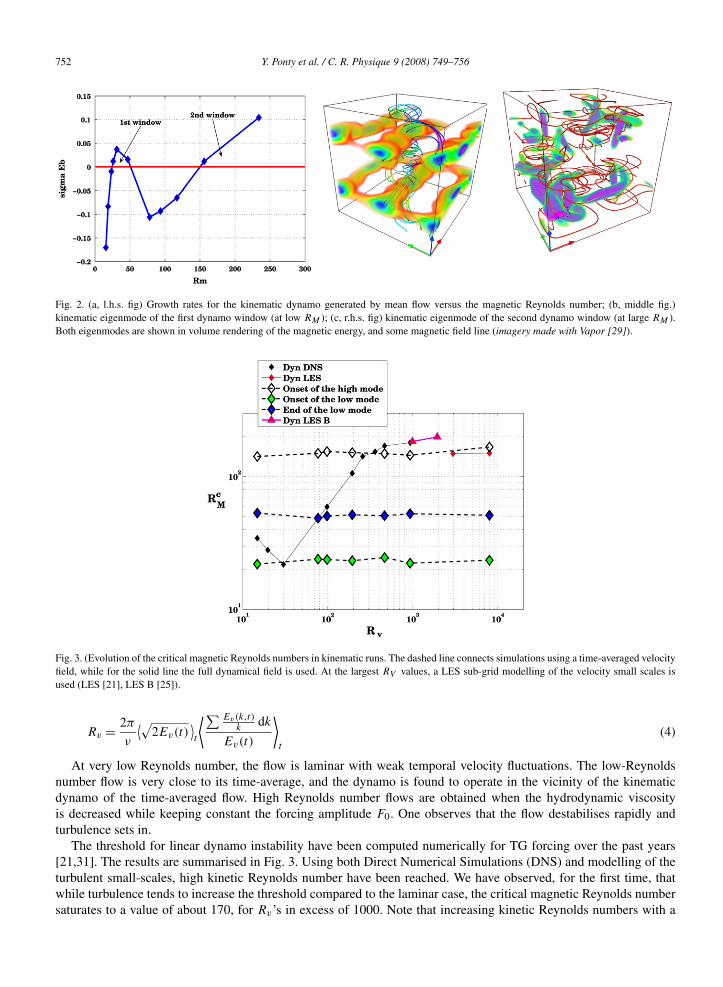
The dynamo capacity of this time-average flow can be analysed in kinematic dynamo computations. Fig. 2(a)shows a typical evolution of the growth rate of magnetic energy (starting from a seed field). One observes two regionsof magnetic Reynolds numbers with positive growth rates – i.e. dynamo branches [31,32,30]. The first dynamo modeevolves at larger scales than the fundamental TG box – Fig. 2(b); it operates in a range of magnetic Reynolds numbers20 < Rm < 50. The second dynamo mode develops within the fundamental box – Fig. 2(c) – for magnetic Reynoldsnumbers in excess of about 180. Its shape is similar to the one obtained in kinematic simulation for the Von Kàrmàntime-averaged velocity field [33,34].

3.2. Kinematic dynamo regime at high Reynolds number

In this section, we study dynamo action from the dynamical velocity fields in the numerical simulations. TheReynolds number is computed using the average in time – labelled 〈·〉t – of the root mean square velocity, and theintegral scale is calculated from the one-dimensional energy spectra Ev(k),


Fig. 2. (a, l.h.s. fig) Growth rates for the kinematic dynamo generated by mean flow versus the magnetic Reynolds number; (b, middle fig.)kinematic eigenmode of the first dynamo window (at low RM ); (c, r.h.s. fig) kinematic eigenmode of the second dynamo window (at large RM ).Both eigenmodes are shown in volume rendering of the magnetic energy, and some magnetic field line (imagery made with Vapor [29]).

Fig. 3. (Evolution of the critical magnetic Reynolds numbers in kinematic runs. The dashed line connects simulations using a time-averaged velocityfield, while for the solid line the full dynamical field is used. At the largest RV values, a LES sub-grid modelling of the velocity small scales isused (LES [21], LES B [25]).

Rv = 2π

ν

⟨√2Ev(t)

⟩t

⟨∑ Ev(k,t)k

dk

Ev(t)

⟩t

(4)

At very low Reynolds number, the flow is laminar with weak temporal velocity fluctuations. The low-Reynoldsnumber flow is very close to its time-average, and the dynamo is found to operate in the vicinity of the kinematicdynamo of the time-averaged flow. High Reynolds number flows are obtained when the hydrodynamic viscosityis decreased while keeping constant the forcing amplitude F0. One observes that the flow destabilises rapidly andturbulence sets in.

The threshold for linear dynamo instability have been computed numerically for TG forcing over the past years[21,31]. The results are summarised in Fig. 3. Using both Direct Numerical Simulations (DNS) and modelling of theturbulent small-scales, high kinetic Reynolds number have been reached. We have observed, for the first time, thatwhile turbulence tends to increase the threshold compared to the laminar case, the critical magnetic Reynolds numbersaturates to a value of about 170, for Rv’s in excess of 1000. Note that increasing kinetic Reynolds numbers with a


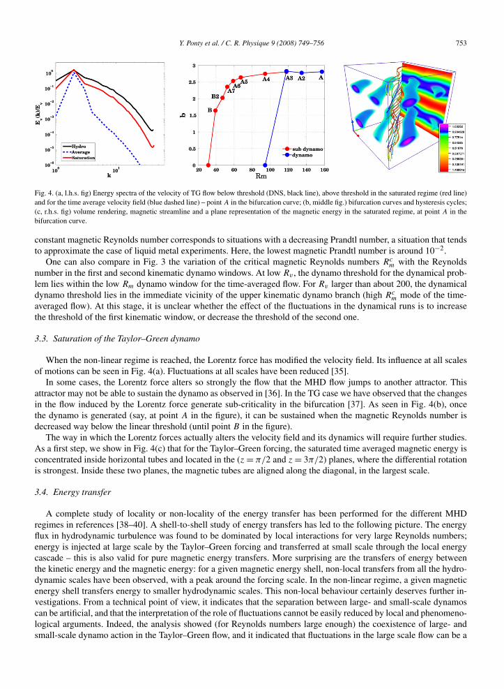
Fig. 4. (a, l.h.s. fig) Energy spectra of the velocity of TG flow below threshold (DNS, black line), above threshold in the saturated regime (red line)and for the time average velocity field (blue dashed line) – point A in the bifurcation curve; (b, middle fig.) bifurcation curves and hysteresis cycles;(c, r.h.s. fig) volume rendering, magnetic streamline and a plane representation of the magnetic energy in the saturated regime, at point A in thebifurcation curve.

constant magnetic Reynolds number corresponds to situations with a decreasing Prandtl number, a situation that tendsto approximate the case of liquid metal experiments. Here, the lowest magnetic Prandtl number is around 10−2.

One can also compare in Fig. 3 the variation of the critical magnetic Reynolds numbers Rcm with the Reynolds

number in the first and second kinematic dynamo windows. At low Rv , the dynamo threshold for the dynamical prob-lem lies within the low Rm dynamo window for the time-averaged flow. For Rv larger than about 200, the dynamicaldynamo threshold lies in the immediate vicinity of the upper kinematic dynamo branch (high Rc

m mode of the time-averaged flow). At this stage, it is unclear whether the effect of the fluctuations in the dynamical runs is to increasethe threshold of the first kinematic window, or decrease the threshold of the second one.

3.3. Saturation of the Taylor–Green dynamo

When the non-linear regime is reached, the Lorentz force has modified the velocity field. Its influence at all scalesof motions can be seen in Fig. 4(a). Fluctuations at all scales have been reduced [35].

In some cases, the Lorentz force alters so strongly the flow that the MHD flow jumps to another attractor. Thisattractor may not be able to sustain the dynamo as observed in [36]. In the TG case we have observed that the changesin the flow induced by the Lorentz force generate sub-criticality in the bifurcation [37]. As seen in Fig. 4(b), oncethe dynamo is generated (say, at point A in the figure), it can be sustained when the magnetic Reynolds number isdecreased way below the linear threshold (until point B in the figure).

The way in which the Lorentz forces actually alters the velocity field and its dynamics will require further studies.As a first step, we show in Fig. 4(c) that for the Taylor–Green forcing, the saturated time averaged magnetic energy isconcentrated inside horizontal tubes and located in the (z = π/2 and z = 3π/2) planes, where the differential rotationis strongest. Inside these two planes, the magnetic tubes are aligned along the diagonal, in the largest scale.

3.4. Energy transfer

A complete study of locality or non-locality of the energy transfer has been performed for the different MHDregimes in references [38–40]. A shell-to-shell study of energy transfers has led to the following picture. The energyflux in hydrodynamic turbulence was found to be dominated by local interactions for very large Reynolds numbers;energy is injected at large scale by the Taylor–Green forcing and transferred at small scale through the local energycascade – this is also valid for pure magnetic energy transfers. More surprising are the transfers of energy betweenthe kinetic energy and the magnetic energy: for a given magnetic energy shell, non-local transfers from all the hydro-dynamic scales have been observed, with a peak around the forcing scale. In the non-linear regime, a given magneticenergy shell transfers energy to smaller hydrodynamic scales. This non-local behaviour certainly deserves further in-vestigations. From a technical point of view, it indicates that the separation between large- and small-scale dynamoscan be artificial, and that the interpretation of the role of fluctuations cannot be easily reduced by local and phenomeno-logical arguments. Indeed, the analysis showed (for Reynolds numbers large enough) the coexistence of large- andsmall-scale dynamo action in the Taylor–Green flow, and it indicated that fluctuations in the large scale flow can be a


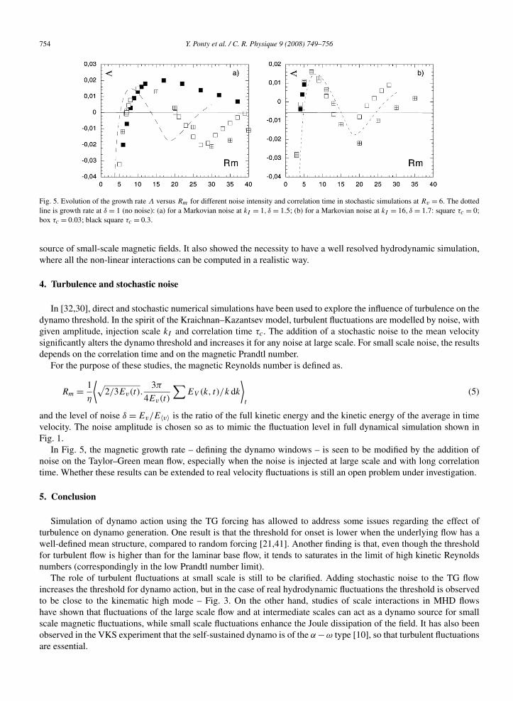
Fig. 5. Evolution of the growth rate Λ versus Rm for different noise intensity and correlation time in stochastic simulations at Rv = 6. The dottedline is growth rate at δ = 1 (no noise): (a) for a Markovian noise at kI = 1, δ = 1.5; (b) for a Markovian noise at kI = 16, δ = 1.7: square τc = 0;box τc = 0.03; black square τc = 0.3.

source of small-scale magnetic fields. It also showed the necessity to have a well resolved hydrodynamic simulation,where all the non-linear interactions can be computed in a realistic way.

4. Turbulence and stochastic noise

In [32,30], direct and stochastic numerical simulations have been used to explore the influence of turbulence on thedynamo threshold. In the spirit of the Kraichnan–Kazantsev model, turbulent fluctuations are modelled by noise, withgiven amplitude, injection scale kI and correlation time τc. The addition of a stochastic noise to the mean velocitysignificantly alters the dynamo threshold and increases it for any noise at large scale. For small scale noise, the resultsdepends on the correlation time and on the magnetic Prandtl number.

For the purpose of these studies, the magnetic Reynolds number is defined as.

Rm = 1

η

⟨√2/3Ev(t).

3π

4Ev(t)

∑EV (k, t)/k dk

⟩t

(5)

and the level of noise δ = Ev/E〈v〉 is the ratio of the full kinetic energy and the kinetic energy of the average in timevelocity. The noise amplitude is chosen so as to mimic the fluctuation level in full dynamical simulation shown inFig. 1.

In Fig. 5, the magnetic growth rate – defining the dynamo windows – is seen to be modified by the addition ofnoise on the Taylor–Green mean flow, especially when the noise is injected at large scale and with long correlationtime. Whether these results can be extended to real velocity fluctuations is still an open problem under investigation.

5. Conclusion

Simulation of dynamo action using the TG forcing has allowed to address some issues regarding the effect ofturbulence on dynamo generation. One result is that the threshold for onset is lower when the underlying flow has awell-defined mean structure, compared to random forcing [21,41]. Another finding is that, even though the thresholdfor turbulent flow is higher than for the laminar base flow, it tends to saturates in the limit of high kinetic Reynoldsnumbers (correspondingly in the low Prandtl number limit).

The role of turbulent fluctuations at small scale is still to be clarified. Adding stochastic noise to the TG flowincreases the threshold for dynamo action, but in the case of real hydrodynamic fluctuations the threshold is observedto be close to the kinematic high mode – Fig. 3. On the other hand, studies of scale interactions in MHD flowshave shown that fluctuations of the large scale flow and at intermediate scales can act as a dynamo source for smallscale magnetic fluctuations, while small scale fluctuations enhance the Joule dissipation of the field. It has also beenobserved in the VKS experiment that the self-sustained dynamo is of the α −ω type [10], so that turbulent fluctuationsare essential.


Some information about the mechanisms which drive the dynamo saturation in the non-linear regime have been ob-tained. In particular, the shell-to-shell energy transfer analysis reveals the non-locality of the energy transfer betweenthe fluid and the magnetic field. This must be taken into account in further studies and models.

Finally, the observed subcriticality in the Taylor–Green dynamo may be is promising for experiments and modellingof natural dynamos (it has been observed in numerical models of the geodynamo as well [42–44]), and indications ofsubcriticality have been observed in the VKS experiment [45].

We still need much effort to reach realistic numerical simulations at high Reynolds numbers inside bounded do-mains. In the mean time, studies in open periodic boxes and pseudo-spectral method remain a convenient numericaltool to study the turbulent dynamo.

Acknowledgements

The French authors thank CNRS Dynamo GdR, CNRS Turbulence GdR, INSU/PNST and INSU/PCMI Programs,“programme de Planétologie”. A.A. acknowledged the financial support of Observatoire de la Côte d’Azur and theRotary Club district 1730. The NSF grant CMG-0327888 is gratefully acknowledged by the USA authors. P.D.M.is a member of the Carrera del Investigador Científico of CONICET. Y.P. thanks A. Miniussi for computing designassistance. Computer time was provided by IDRIS, the Mesocentre SIGAMM machine, hosted by Observatoire de laCote d’Azur, NCAR and Pittsburg Supercomputing center.

References

[1] H.K. Moffatt, Magnetic Field Generation in Electrically Conducting Fluids, Cambridge University Press, Cambridge, 1978;E.N. Parker, Cosmical Magnetic Fields, Clarendon Press, Oxford, 1979.

[2] P. Odier, J.-F. Pinton, S. Fauve, Advection of a magnetic field by a turbulent swirling flow, Phys. Rev. E 58 (1998) 7397–7401.[3] N.L. Peffley, A.B. Cawthorne, D.P. Lathrop, Toward a self-generating magnetic dynamo, Phys. Rev. E 61 (2000) 5287.[4] M. Bourgoin, L. Marié, F. Pétrélis, C. Gasquet, A. Guiguon, J.-B. Luciani, M. Moulin, F. Namer, J. Burguete, F. Daviaud, A. Chiffaudel,

S. Fauve, Ph. Odier, J.-F. Pinton, MHD measurements in the von Kármán sodium experiment, Phys. Fluids 14 (2002) 3046.[5] M.D. Nornberg, E.J. Spence, R.D. Kendrick, C.M. Jacobson, C.B. Forest, Intermittent magnetic field excitation by a turbulent flow of liquid

sodium, Phys. Rev. Lett. 97 (2006) 044503.[6] R. Stepanov, R. Volk, S. Denisov, P. Frick, V. Noskov, J.-F. Pinton, Induction, helicity, and alpha effect in a toroidal screw flow of liquid

gallium, Phys. Rev. E 73 (2006) 046310.[7] R. Volk, P. Odier, J.-F. Pinton, Fluctuation of magnetic induction in von Kármán swirling flows, Phys. Fluids 18 (2006) 085105.[8] A. Gailitis, O. Lielausis, S. Dement’ev, A. Cifersons, G. Gerbeth, T. Gundrum, F. Stefani, M. Christen, H. Hãnel, G. Will, Magnetic field

saturation in the Riga dynamo experiment, Phys. Rev. Lett. 86 (2001) 3024.[9] R. Stieglitz, U. Müller, Experimental demonstration of a homogeneous two-scale dynamo, Phys. Fluids 13 (2001) 561.

[10] R. Monchaux, M. Berhanu, M. Bourgoin, M. Moulin, Ph. Odier, J.-F. Pinton, R. Volk, S. Fauve, N. Mordant, F. Pétrélis, A. Chiffaudel,F. Daviaud, B. Dubrulle, C. Gasquet, L. Marié, F. Ravelet, Generation of a magnetic field by dynamo action in a turbulent flow of liquidsodium, Phys. Rev. Lett. 98 (2007) 044502.

[11] M. Berhanu, R. Monchaux, S. Fauve, N. Mordant, F. Pétrélis, A. Chiffaudel, F. Daviaud, F. Ravelet, M. Bourgoin, Ph. Odier, J.-F. Pinton,R. Volk, B. Dubrulle, L. Marie, Magnetic field reversals in an experimental turbulent dynamo, Europhys. Lett. 77 (2007) 59001.

[12] J.L. Guermond, J. Léorat, C. Nore, A new finite Element Method for magneto-dynamical problems: two-dimensional results, Eur. J. Mech.B/Fluids 22 (2003) 555.

[13] A.B. Iskakov, S. Descombes, E. Dormy, An integro-differential formulation for magnetic induction in bounded domains: boundary element-finite volume method, J. Comput. Phys. 197 (2004) 540–554.

[14] J.L. Guermond, R. Laguerre, J. Léorat, C. Nore, An interior penalty Galerkin method for the MHD equations in heterogeneous domains,J. Comput. Phys. 221 (2007) 349–369.

[15] U. Frisch, Turbulence: The Legacy of A.N. Kolmogorov, Cambridge University Press, 1996.[16] S.A. Orszag, J.S. Patterson Jr, Numerical simulation of three-dimensional homogeneous isotropic turbulence, Phys. Rev. Lett. 28 (1972)

76–79.[17] A. Vincent, M. Meneguzzi, The spatial structure and the statistical properties of homegeneous turbulence, J. Fluid Mech. 225 (1991) 1–25.[18] M.E. Brachet, D.I. Meiron, S.A. Orszag, B.G. Nickel, R.H. Morf, U. Frisch, Small-scale structure of the Taylor–Green vortex, J. Mech.

Fluids 130 (1983) 411–452.[19] M. Lesieur, Turbulence in Fluids, Kluwer, 1997.[20] Y. Ponty, J.F. Pinton, H. Politano, Simulation of induction at low magnetic Prandtl number, Phys. Rev. Lett. 92 (14) (2004) 144503.[21] Y. Ponty, P.D. Minnini, A. Pouquet, H. Politano, D.C. Montgomery, J.-F. Pinton, Numerical study of dynamo action at low magnetic Prandtl

numbers, Phys. Rev. Lett. 94 (2005) 164512.[22] D.C. Montgomery, A. Pouquet, An alternative interpretation for the Holm alpha model, Phys. Fluids 14 (2002) 3365.[23] P.D. Mininni, D.C. Montgomery, A. Pouquet, Numerical solutions of the three-dimensional magnetohydrodynamic alpha model, Phys.

Rev. E 71 (2005) 046304.


[24] J. Baerenzung, H. Politano, Y. Ponty, A. Pouquet, Spectral modeling of turbulent flows and the role of helicity, Phys. Rev. E 77 (2008) 046303.[25] J. Baerenzung, H. Politano, Y. Ponty, A. Pouquet, Spectral modeling of magnetohydrodynamic turbulent flows, Phys. Rev. E (2008), in press.[26] S. Douady, Y. Couder, M.-E. Brachet, Direct observation of the intermittency of intense vorticity filaments in turbulence, Phys. Rev. Lett. 67

(1991) 983.[27] C. Nore, M. Brachet, H. Politano, A. Pouquet, Dynamo action in the Taylor–Green vortex near threshold, Phys. Plasmas 4 (1997) 1.[28] C. Nore, M.-E. Brachet, H. Politano, A. Pouquet, Dynamo action in a forced Taylor–Green vortex, in: P. Chossat, D. Armbruster, I. Oprea

(Eds.), Dynamo and Dynamics, a Mathematical Challenge, Cargèse, France, 21–26 August 2000, in: Nato Science Series II, vol. 26, KluwerAcademic, Dordrecht, 2001, pp. 51–58. Proceedings of the Nato Advanced Research Workshop.

[29] J. Clyne, P.D. Mininni, A. Norton, M. Rast, Interactive desktop analysis of high resolution simulations: application to turbulent plume dynam-ics and current sheet formation, New J. Phys. 9 (2007) 301.

[30] B. Dubrulle, P. Blaineau, O. Mafra Lopes, F. Daviaud, J.-P. Laval, R. Dolganov, Bifurcations and dynamo action in a Taylor–Green flow, NewJ. Phys. 9 (2007) 308.

[31] Y. Ponty, P.D. Minnini, J.-F. Pinton, H. Politano, A. Pouquet, Dynamo action at low magnetic Prandtl numbers: mean flow versus fullyturbulent motions, New J. Phys. 9 (2007) 296.

[32] J.-P. Laval, P. Blaineau, N. Leprovost, B. Dubrulle, F. Daviaud, Influence of turbulence on the dynamo threshold, Phys. Rev. Lett. 96 (2006)204503.

[33] L. Marié, J. Burgete, F. Daviaud, J. Léorat, Numerical study of homogeneous dynamo based on experimental von Karman type flows, Eur.Phys. J. B 33 (2003) 469.

[34] F. Ravelet, A. Chiffaudel, F. Daviaud, J. Léorat, Toward an experimental von Kármán dynamo: Numerical studies for an optimized design,Phys. Fluids 17 (2005) 117104.

[35] P.D. Mininni, Y. Ponty, D.C. Montgomery, J.-F. Pinton, H. Politano, A. Pouquet, Dynamo regimes with a non-helical forcing, Astrophys. J.626 (2005) 853–863.

[36] N.H. Brummell, F. Cattaneo, S.M. Tobias, Linear and nonlinear dynamo properties of time-dependent ABC flows, Fluid Dynam. Res. 28(2001) 237–265.

[37] Y. Ponty, J.-P. Laval, B. Dubrulle, F. Daviaud, J.-F. Pinton, Subcritical dynamo bifurcation in the Taylor–Green flow, Phys. Rev. Lett. 99(2007) 224501.

[38] A. Alexakis, P.D. Mininni, A. Pouquet, Shell-to-shell energy transfer in magnetohydrodynamics. I. Steady state turbulence, Phys. Rev. E 72(2005) 046301.

[39] P. Mininni, A. Alexakis, A. Pouquet, Shell-to-shell energy transfer in magnetohydrodynamics. II. Kinematic dynamo, Phys. Rev. E 72 (2005)046302.

[40] A. Alexakis, P.D. Mininni, A. Pouquet, Turbulent cascades, transfer, and scale interactions in magnetohydrodynamics, New J. Phys. 9 (2007)298.

[41] A.A. Schekochihin, A.B. Iskakov, S.C. Cowley, J.C. McWilliams, M.R.E. Proctor, T.A. Yousef, Fluctuation dynamo and turbulent inductionat low magnetic Prandtl numbers, New J. Phys. 9 (2007) 300.

[42] U.R. Christensen, P. Olson, G.A. Glatzmaier, Numerical modeling of the geodynamo: A systematic parameter study, Geophys. J. Int. 138(1999) 393.

[43] S. Stellmach, U. Hansen, Cartesian convection driven dynamos at low Ekman number, Phys. Rev. E 70 (2004) 056312.[44] V. Morin, Ph.D. Thesis, University Paris VI, 2005.[45] M. Berhanu, R. Monchaux, M. Bourgoin, Ph. Odier, J.-F. Pinton, N. Plihon, R. Volk, S. Fauve, N. Mordant, F. Pétrélis, S. Aumaître, A. Chif-

faudel, F. Daviaud, B. Dubrulle, F. Ravelet, Bistability between a stationary and an oscillatory dynamo in a turbulent flow of liquid sodium,Europhys. Lett. (03/2008), submitted for publication.

Linear and non-linear features of the Taylor–Green dynamo

Documents

Transcript of Linear and non-linear features of the Taylor–Green dynamo