BioSystems 91 (2008) 558–571

Available online at www.sciencedirect.com

Simulation of a bounded symport/antiport P systemwith Brane calculi

Antonio Vitale ∗, Giancarlo Mauri, Claudio ZandronUniversita degli Studi di Milano-Bicocca, Dipartimento di Informatica, Sistemistica e Comunicazione,

Via Bicocca degli Arcimboldi 8, 20126 Milano, Italy

Received 31 March 2006; received in revised form 16 November 2006; accepted 29 January 2007

Abstract

Membrane systems (also called P systems) and Brane calculi have been recently introduced as formal models inspired by thestructure and the functioning of living cells, but having in mind different goals. The aim of Membrane systems was the formalinvestigation of the computational nature and power of various features of the cell, while Brane calculi aims to define a modelcapable of a faithful and intuitive representation of various biological processes.

The common background of the two formalisms and the recent growing of interests in applying P systems in Systems Biologyhave raised the natural question of bridging this two research areas. The present paper goes in this direction, as it presents a directsimulation of a variant of P systems by means of Brane calculi. In particular, we consider a Brane calculus based on three operations

called Mate/Bud/Drip, and we show how to use such system to simulate Simple symport/antiport P systems, a variant of P systemspurely based on communication of objects. As an example, a simplified sodium–potassium pump modeled in Simple SA is encodedin Mate/Bud/Drip Brane calculus.© 2007 Elsevier Ireland Ltd. All rights reserved.

Keywords: Membrane computing; Brane calculi; Systems Biology

1. Introduction

Both P systems (Paun, 1998, 1999, 2002, 2003, 2004)and Brane calculi (Cardelli, 2004) have been introducedas (families of) computational models inspired by thestructure and the functioning of the living cell, start-ing from the key observation that the various processes

taking place in the living cell can be regarded as compu-tations.

∗ Corresponding author.E-mail addresses: antonio.vitale@studenti.unimib.it (A. Vitale),

mauri@disco.unimib.it (G. Mauri), zandron@disco.unimib.it(C. Zandron).

0303-2647/$ – see front matter © 2007 Elsevier Ireland Ltd. All rights reservdoi:10.1016/j.biosystems.2007.01.008

Although they have common bases, they have dif-ferent goals: the main objective of P system’s (Thep systems web page, http://psystems.disco.unimib.it/)area of research is the formal investigation of the com-putational nature and power of various features ofmembranes, while Brane calculi’s main goal is to createa model capable of a faithful and intuitive representationof the biological reality.

To better clarify the different goals we quote fromCardelli and Paun (2005):

“While membrane computing (i.e. P systems) is a

branch of natural computing, which tries to abstractcomputing models, in the Turing sense, from thestructure and the functioning of the cell, making useespecially of automata, languages, and complexity

ed.

ystems

ccmFrcenoie

mntwTs

acmmbgpew

tcncnsmcbsilt

bla

A. Vitale et al. / BioS

theoretic tools, Brane calculi pay more attention to thefidelity to the biological reality, have as primary targetsystems biology, and use especially the framework ofprocess algebra.”

Living cells are extremely well organized self-ontained systems, composed by discrete interactingomponents. Each component is delimited by a physicalembrane and is often called region or compartment.rom a computer science point of view, we can surelyegard the cells as information processing devices. Aell has a complex internal activity and an ingeniouslylaborated interactions with the environment and theeighbouring cells. A proper interaction based on a flowf substances between components and the environments necessary for the cell life: a cell not aware of thenvironment conditions soon dies.

In P systems the cell organization is simulated by aembrane structure formalized with a Venn diagram ofested membranes, while the chemicals swimming inhe solution delimited by a compartment are representedith a multiset of symbols/objects from a given alphabet.he multiset notion perfectly simulates the unorderedtructure of floating chemicals.

In the basic variant of P systems the objects evolveccording to evolution rules, locally associated to theompartments, that transform multisets of symbols inultisets of symbols. The interaction between compart-ents is realized by evolution rules that move objects

etween directly nested membranes. Such rules areenerally applied non deterministically in a maximallyarallel manner: the rules to be used and the objects tovolve are randomly chosen, and, in each step all objectshich can evolve must do it.While in Brane calculi we have a membrane struc-

ure too, membranes are not simple separators ofompartments as in P systems but they are coordi-ators and active sites of major activity. In Branealculi a computation happens on the membrane andot inside of it. So we no longer make use of multi-ets of objects but work with processes that reside onembranes. The operations of the two basic Brane cal-

uli proposed in Cardelli (2004) are directly inspiredy biologic processes such as endocytosis, exocyto-is and mitosis. Another difference with P systemss that generally Brane calculi evolve using an inter-eaving semantics (sequential single instruction execu-ion).

Only recently P systems have been applied to modeliological systems and processes (in particular at cellularevel). The common background of the two formalismsnd the recent shift of interests of P systems toward Sys-

91 (2008) 558–571 559

tem Biology have raised the natural question of bridgingthe two research areas.

Various formal results have already been achieved.In Busi and Gorrieri (2005) the computational power oftwo basic Brane calculi proposed in Cardelli (2004) isinvestigated. In Cardelli and Paun (2005) is inspecteda variant of P systems inspired by the interactions of abasic Brane calculus defined in Cardelli (2004). A paral-lel semantics for Brane calculi, inspired by the maximalparallelism semantics of P systems, is considered in Busi(2005). Finally in Paun (2005) two variants of P systemswhose interactions are inspired by the two basic Branecalculi defined in Cardelli (2004) are studied.

This paper follows these recent attempts to connectP systems with Brane calculi, and it contributes with astraight simulation of a variant of P systems by meansof Brane calculi. In particular, we consider the vari-ant of Brane calculi based on three operations calledMate/Bud/Drip (Cardelli, 2004): such primitives areinspired by membrane fusion (mate) and fission (mito).The fission process is modelled by both Bud and Dripoperations: the former consists in splitting off exactlyone internal membrane while the latter in splitting offzero internal membrane.

We will show how Mate/Bud/Drip Brane calculus(MBD) can be used to simulate Simple SA systems(Ibarra et al., in press), a bounded variant of P systemswith symport/antiport rules (Paun and Paun, 2002) wherecomputations are purely based on communication ofobjects. Such systems are closely related to the biologictrans-membrane communication by coupling chemicalsand do not evolve by transforming objects, as the basicvariant of P systems, but by changing their position withrespect to the compartments defined by the membranestructure used.

The rest of the paper is organized as follows. In Sec-tion 2 we introduce all the formal notions we will needin the rest of the paper. Section 3 contains the descrip-tion of the simulation of Simple SA systems in the MDBBrane calculus. In Section 4 we show an example of atranslation: we encode a simplified sodium–potassiumpump modeled in Simple SA in MDB Brane calculus.In Section 5 we report some final remarks and we givesome perspectives for future work.

2. Preliminaries

The notions of formal language theory we use are

basic, and can be found in every monograph in this area(e.g. Rozenberg and Salomaa, 1997).

The key function of a biological membrane in a livingcell is to define a compartment and its interaction with

560 A. Vitale et al. / BioSystems 91 (2008) 558–571

tructure

Fig. 1. Three equivalent ways to represent the same membrane s

the surrounding environment (including other compart-ments). In both P systems and Brane calculi we have amembrane structure where the membrane concept is usedas a logic separator between processes and resources.The membrane structure can be seen as a tree like struc-ture, a Venn diagram or a correctly matching parenthesesstring and it should be clear that we can have nestedmembrane structures. The most external membrane of asystem is called skin membrane and a membrane not con-taining other membranes it is said to be elementary. Thespace defined by a membrane is called region or compart-ment. A biologic membrane contains various substancesand we use the multiset notion to formalize them. Amultiset W over a set X is a mapping W : X → N andcan be represented with a string (e.g. a3bc2 = abacac =baccaa = . . .). The multiset data structure let us directlyformalize the multiplicities and the unordered structureof floating chemicals.

2.1. P Systems

P systems aim to abstract new computing paradigmsfrom the biological reality of living cells using tools fromthe field of automata and formal language theory. Gen-erally speaking a P system is a computational modelbased on a membrane structure (Fig. 1)1 and processeslocally multisets of symbols in a parallel and distributedmanner. Each membrane identifies a compartment (orregion) that c ontains a set of evolution rules and a mul-tiset of symbols from a given alphabet. The symbols ineach compartment evolve according to the set of rulescontained in it. Typically the rules are used in a nondeterministic, maximally parallel way; at each step ofcomputation rules and objects (symbols) are associated

in a non deterministic way until no further choice canbe made and then the rules are simultaneously appliedto the assigned symbols. A computation is successfulif it halts and a simple way to define the output is to

1 Usually a hierarchical structure as shown in Fig. 1, but a net struc-ture exists too.

: (a) Venn diagram, (b) Tree like and (c) Matching parentheses.

consider the number of objects in a predefined compart-ment.

One of the most interesting classes of P systems is thesymport /antiport one, first introduced in Paun and Paun(2002). P systems with symport/antiport rules (brieflyS/A P systems) are closely related to the biological trans-membrane communication that occurs at the cellularlevel and relies on coupling chemicals. When two chem-icals can cross a membrane only together in the samedirection we speak of symport process; when the twochemicals can cross a membrane only together but inopposite direction we speak of antiport process. Givenan alphabet of objects V and objects a, b ∈ V we for-malize these processes with rules of the form (ab, in) or(ab, out) for symport and (a, out; b, in) for antiport. Wealso consider rules of the form (a, in) or (a, out) and callthem u niport rules.

A system with only these rules is purely communica-tive since no objects are destroyed or transformed duringthe computation, they only change the compartment theybelong to. Formally a S/A P system is a constructΠ = (V, μ, W1, . . . , Wm, E, R1, . . . , Rm, i0)

where: V is the alphabet of objects; μ is a membranestructure with m membranes injectively labelled by pos-itive integers 1, 2, . . . , m; W1, . . . , Wm are the multisetsof objects (symbols) initially contained in the compart-ments; E ⊆ V is the set of objects present in arbitrarilymany copies in the environment; R1, . . . , Rm are finitesets of rules associated with the m membranes of μ;i0 ∈ {1, . . . , m} is an elementary membrane of μ (theoutput membrane). The c onfiguration of a S/A P systemis defined by the multisets of objects present in all theregions of Π. The result of a S/A P system is the num-ber of objects present in the membrane (compartment)labelled i0 in the halting configuration.

2.1.1. Simple SAA Simple SA2 (of degree k + 1) is a limited (i.e. non

universal) variant of a S/A P system, and is defined by a

2 Obviously “SA” stands for “symport/antiport”.

ystems

c

Π

w

•

•

•

•

•

aibss

fpSomor

2

fb

hto

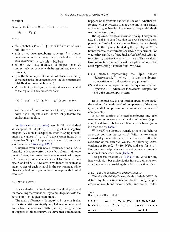
2.2.1. The Mate/Bud/Drip Brane CalculusThe Mate/Bud/Drip Brane calculus (briefly MDB) is

defined by three actions inspired by the biological pro-cesses of membrane fusion (mate) and fission (mito).

Table 1Basic syntax of Brane calculi

A. Vitale et al. / BioS

onstruct

= (V, μ, W1, . . . , Wk+1, WE, n1, . . . , nk,

R1, . . . , Rk+1)

here

the alphabet is V = F ∪ {o} with F finite set of sym-bols and o /∈ F ;μ is a two level membrane structure: k ≥ 1 inputmembranes on the same level embedded in askin membrane → [skin[1]1· · ·[k]k]skin;Wi, WE are finite multisets of objects over F,respectively, associated with the region i and the envi-ronment;ni is the (non negative) number of objects o initiallycontained in the input membrane i (the skin membraneinitially does not contain any o);Ri is a finite set of symport/antiport rules associatedto the region i. They are of the form

·(a) (u, out) · (b) (v, in) · (c) (u, out; v, in)

with u, v ∈ V+, and for rules of type (b) and (c) itholds o /∈ v: objects o can “move” only toward theenvironment region.

In Ibarra et al. (in press) Simple SA are studieds acceptors of k-tuples (n1, . . . , nk) of non negativentegers. A k-tuple is accepted if, when the k input mem-ranes are given on1 , . . . , onk , the system halts. It ishown that Simple SA systems characterize exactly theemilinear sets (Ginsburg, 1966).

Compared with basic S/A P systems, Simple SA isormally a less powerful device but, from a biologicoint of view, the limited resources scenario of SimpleA makes it a more realistic model for System Biol-gy. Standard S/A P systems have indeed uncountableany copies of each symbol in the environment while

bviously biologic systems have to cope with limitedesources.

.2. Brane Calculi

Brane calculi are a family of process calculi proposedor modelling the various cell dynamics together with theehaviour of biological membranes.

The main difference with regard to P systems is thatere active entities are tightly coupled to membranes andhis endows membranes with the (correct) biological rolef support of biochemistry; we have that computation

91 (2008) 558–571 561

happens on membrane and not inside of it. Another dif-ference with P systems is that generally Brane calculievolve using an interleaving semantic (sequential singleinstruction execution).

Biologic membranes are formed by a lipid bilayer thatactually behaves as a fluid that let both structural com-ponents and embedded substances like proteins to freelymove into the region delimited by the lipid layers. Mem-branes themselves are immersed into an aqueous solutionwhere they can freely float. Such a fluid within fluid struc-ture directly inspires the basic structure of Brane calculi:two commutative monoids with a replication operator,each representing a kind of fluid. We have

(1) a monoid representing the lipid bilayer:(Membranes, |, 0) where | is the membranes’composition and 0 the unit (empty process);

(2) and a monoid representing the aqueous solution:(Systems, ◦, ) where ◦ is the systems’ compositionand the unit (empty system).

Both monoids use the replication operator ! to modelthe notion of a “multitude” of components of the sametype (parallel composition of an unbounded number ofcomponents).

A system consists of nested membranes and eachmembrane represents a combination of actions (a pro-cess) that define its behaviour. Formally the basic syntaxis described by Table 1.

With σ〈P〉 we denote a generic system that behavesas σ and contains the system P. With a.σ we denotea guarded process: the process behaves as σ after theexecution of the action a. We use the following abbre-viations: a for a.0, 〈P〉 for 0〈P〉, and σ〈〉 for σ〈 〉.Both systems and processes have a structural congruencerelation defined over them (Table 2).

The generic reactions of Table 3 are valid for anyBrane calculus, but each calculus have to define its ownspecific reactions providing the relative reaction rules.

562 A. Vitale et al. / BioSystems

Table 2Structural congruence relation for systems and membranes

Table 3Generic reaction rules

a Roughly speaking this means that the reaction is not an elementarytransition but is composed by a sequence of elementary reactions.

The fission process is specialized into two operations:budding (bud), which consists in the splitting off oneinternal membrane, and dripping (drip), which consistsin the splitting off zero internal membranes. The fusionprocess is represented by the mating (mate) operation.Tables 4 and 5 provide the MDB actions’ syntax andreaction rules.

For actions that involve two membranes we need a co-action to identify the second membrane. Such co-actionsare obtained appending the symbol⊥ to the action name.Moreover we can index our actions in order to preciselycouple an action with the correct co-action.

Actions mate and mate⊥ will synchronize to

n n

achieve membranes fusion and the membranes will resultirreversible mixed. Actions budn and bud⊥

n will syn-chronize to split one nested membrane. Action drip let

Table 4MDB actions’ syntax

Actions a,b : :=maten | mate⊥n | budn | bud⊥(ρ) | drip(ρ)

Table 5Reaction rules for MDB

91 (2008) 558–571

to split off zero internal membranes. Actions drip andbud⊥ come with a parameter ρ which represents themembrane process of the new membrane created by thereaction.

2.3. MDB Syntax Simplifications

Let k be a positive integer and ω a membrane pro-cess (combinations of actions, see Table 1), we use thefollowing syntax simplifications

k(ω)�k︷ ︸︸ ︷

ω.ω.· · · .ω and (ω)k �k︷ ︸︸ ︷

ω|ω|· · ·|ω

Moreover, where clear enough, we often omit the paren-theses and use just kω and ωk. With indexed membraneprocess we use

∏to denote the parallel composition

k∏i=1

ωi �ω1 | · · · | ωk

and the symbol∑

for

k∑i=1

ωi �ω1.ω2.· · · .ωk

Similarly for parallel composition of k identical systemswe use

(P)k �k︷ ︸︸ ︷

P |P |P |P

where P is a system.

2.4. Synchronization Actions

In order to deal with common synchronization situa-tions for adjacent and directly nested membranes in theMDB calculus, we introduce the composite synchroniza-tion actions syn and syn⊥.

Let us assume we want to model a dependency ofprocess ωB1 from process ωA1 . More generally, let ωB1

and ωA1 be two processes that need to synchronize, withωB1 the process waiting for a signal from ωA1 . ClearlyωA1 and ωB1 must be in parallel.

Although syn and syn⊥ are designed as anaction–coaction couple, they, for their composite nature,

do not happen simultaneously. A syn action is free toexecute whenever able to, while the corresponding syn⊥action can execute only if the former already executed,and between the two, arbitrarily many actions can exe-

ystems

c

FaTbutndi

(

(

(

tgscbp

tC!

sω

d

mally parallel step of execution;• the processes that determine if a certain rule i is appli-

A. Vitale et al. / BioS

ute. We define the following systems

A � ωA1 .synAB | ωA2〈· · ·〉B � syn⊥

AB.ωB1 | ωB2〈· · ·〉(1)

or greater flexibility, we define the synchronizationctions syn and syn⊥ as special contextual operations.hat means they have different definitions determinedy the context (i.e. the membranes involved) they aresed in. While modelling, we can simply regard syn ashe “send signal” action and syn⊥ as the “receive sig-al” action, but it should be clear that we are effectivelyealing with three different couples of definitions. Wendeed have the following scenarios:

1) A and B adjacent:

2) B nested in A:

3) A nested in B:

The further scenario of processes ωA1 and ωB1 onhe same membrane in parallel composition is analo-ous to the scenario of adjacent membranes: the coupleynsyn⊥ is defined the same way, and so a signal synan be received indistinctly by an adjacent membrane ory a process on the same membrane. We will use thisroperty later in our encoding.

The scenario (2) requires an ad hoc support sys-em C: if the syn action is thought to repeat system

must be present with the proper multiplicity (e.g.syn ⇒!C).

We leave it as an exercise to verify that in all thecenarios considered above the system S can execute

B1 only after executing ωA1 . That realizes our depen-ency:

91 (2008) 558–571 563

3. The Encoding

We now show how to construct a non determinis-tic simulation of Simple SA with MDB calculus. Theencoding we propose is non deterministic in the follow-ing sense: the simulation behaves non deterministicallyonly when the original (simulated) Simple SA systemshows non deterministic behaviour too.

Let Π be the Simple SA system we want to simulate,we call H the set of all available objects3 in Π. We havethat

|H | = h =k+1∑j=1

|Wj| + |WE| +k∑

j=1

|onj | (2)

and moreover

(1) H is finite;(2) and its cardinality h is fixed for the entire computa-

tion.

The first property is the main characteristic of Sim-ple SA systems and it derives from the finiteness of themultiset WE initially given to the environment E (in abasic S/A P system the environment has an unboundedquantity of specified objects). The second property is adirect consequence of the intrinsic c onservation law ofS/A P systems: no object is created or destroyed duringthe computation. From now on with h we always referto the fixed number of objects of the Simple SA we areconsidering.

It is now easy to formulate a key observation: in asingle step of computation a Simple SA can executeat most h reactions. Indeed, in order to maximize thenumber of rules used having exactly h objects, we can(if all conditions are met) choose for execution h uni-port rules (they “use” only a single object). It is obviousthat after choosing h uniport rules we use all our objectsand no more choices are possible. We recall that eachregion/membrane4 is identified by a unique index i, andwith a little abuse of notation we can identify the envi-ronment with the index k + 2. We also label the rules bya given set of integers in a one to one manner.

The most relevant parts of our encoding are:

• the (exact) simulation of a non deterministic maxi-

cable or not;

3 Including the environment objects.4 Clearly the correspondence region–membrane is one to one.

ystems

564 A. Vitale et al. / BioS

• the way we encode the objects and the membranestructure of Π.

3.1. Encoding Objects and Structure

Given a multiset Wl and an object a ∈ Wl we encodea with the following system

matea,l〈〉This system models an instance of object a contained bythe membrane l. Hence, if Wl = α1, . . . , αs, we modelWl with the following composition of systems

Wl = mateα1,l〈〉 ◦ · · · ◦ mateαs,l〈〉In a similar way we model each o symbol contained bya membrane l with a system

mateo,l〈〉Given a configuration of Π we can easily encode everyobject in the MDB calculus using the above suggestionsobtaining h systems (one for each object of Π) of theform mateβ,i〈〉withβ ∈ V and i ∈ 1, . . . , k + 2. It shouldbe clear enough that a composition of all such systemsembedded in a single membrane would preserve all theinformations of the given Π configuration (the symbolsalong with their position in the membrane structure).

Clearly two objects of the same type generate twodifferent systems if they belong to different regions.Since we have k + 2 regions (we include the environmentregion) each object a ∈ V can map in k + 2 different sys-tems according to its actual region. With such encodingwe effectively collapse the two level structure of Π byexpanding the alphabet used by exactly a k + 2 factor. InMDB we no longer work with objects from V but withobjects from a new alphabet V where

V = {1, 2, . . . , k + 2} × V

It should be clear that each symbol of V has a directinterpretation as an MDB system; a bijection that

∀α ∈ V α �→ mateα〈〉 (3)

It is worth noting that we can similarly collapse astructure of any complexity with the only constraint ofusing an accordingly expanded alphabet. Collapsing astructure of degree m would expand the original alpha-bet V to an alphabet of cardinality |V |(m + 1). We use

H to denote the set of all the encoded objects of Π.For bijection (3) we can interchangeably consider H ascomposed by symbols from V or by systems of the formmateα〈〉 with α ∈ V .

91 (2008) 558–571

3.2. Simulating Rules

Having encoded the data structure we now show howto simulate the symport/antiport rules of Π. Let i be ageneric rule associated to membrane l, it can be exe-cuted only if all the necessary objects are simultaneouslyavailable.

In Simple SA, the verification of the availability ofobjects is directly demanded to the semantics used, whilein Brane calculi we must simulate the verifying process.The only way we can assure the presence of an objectα in region l is to execute the action mate⊥

α,l effec-tively “consuming” the system mateα,l〈〉 that encodesthe object.

Since rule i generally requires a string u ∈ V ∗ the ver-ifying process for i is a sequence of mate⊥ actions.For example, let u = α1, . . . , αn and i = (u, out), wesay that i is executable if we can execute the followingsequence:

mate⊥α1,l

.mate⊥α2,l

. . . . .mate⊥αn,l

(4)

If the sequence (4) completes successfully we can pro-ceed with execution of rule i, but if some object is missingthe sequence halts in a deadlock condition. To prevent aglobal deadlock we compose such process with its coun-terpart: a process that successfully completes if and onlyif there are not all the necessary objects to execute i.These two process are complementary: if one success-fully completes the other will certainly deadlock and viceversa. We call run the process that verifies the presenceof the necessary objects and then executes the rule i,while we call skip the process that verifies the unavail-ability of the necessary objects. Composing in parallelthe two processes we can deterministically establish ifrule i can be executed or not. Before detailing the two pro-cesses we must introduce the concept of complementarysymbols/objects.

3.2.1. Complementary ObjectsWe have already suggested a way to evaluate the exe-

cutability of a rule (i.e. the Eq. (4)) but not how to verifythe contrary (the skip process). Let

λmi,1i,1 λmi,2

i,2 . . . λmi,tii,ti

, λi,j ∈ V , mi,k ∈ N+

be the multiset of objects required by rule i. If wedenote with |H |λi,j the number of occurrences of systemmateλi,j 〈〉 in set H the followings holds

|H |λi,1 ≥ mi,1 ∧ |H |λi,2 ≥ mi,2 ∧ · · · ∧ |H |λi,ti≥ mi,ti

⇔ rule i is applicable (5)

|H |λi,1 < mi,1 ∨ |H |λi,2 < mi,2 ∨ · · · ∨ |H |λi,ti< mi,ti

ystems

WtsbiWw

m

Ia

C

Is

|wotf

|

Ut

h

waascbl.

la

d

A. Vitale et al. / BioS

⇔ rule i is not applicable (6)

e are interested to, and will use, only the (⇒) part ofhe above equations. The interpretation of (5) is quitetraightforward: if the multiplicities of objects requiredy rule i are less or equal to the corresponding multiplic-ties of objects present in H then rule i can be executed.

e already know we can verify the antecedent of (5)ith the following sequence

i,1(mate⊥λi,1

).mi,2(mate⊥λi,2

).· · · .mi,ti (mate⊥λi,ti

)

(7)

n order to verify the antecedent of (6) we define thelphabet of the complementary objects of V

(V ) = {α : α ∈ V }f we add to H systems from {mateα〈〉 : α ∈ C(V )} inuch a way that

H |α + |H |α = h ∀α ∈ V (8)

e have that |H |α corresponds exactly to the numberf systems in H different from mateα〈〉 (not countinghe complementary systems!). Hence we can write theollowing equivalence

H |λi,1 < mi,1 ∨ |H |λi,2 < mi,2 ∨ · · · ∨ |H |λi,ti< mi,ti

= |H |λi,1> h − mi,1 ∨ |H |λi,2

> h − mi,2 ∨ · · ·∨|H |λi,ti

> h − mi,ti (9)

sing (9) we can now verify the antecedent of (6) withhe following composition of processes

1(mate⊥λi,1

) | h2(mate⊥λi,2

) | · · · | hti (mate⊥λi,ti

)

(10)

here hj = (h − mi,j + 1). More precisely thentecedent is verified if any of the ti processes in thebove composition successfully complete. For theake of clarity, we observe that in (10) we use parallelomposition while in (7) we use a straight sequenceecause of the different “normal forms”5 of the twoogic expressions (6) and (5): the former is true if any

. ., while the latter if all . . .. For that reason we willater use the

∑operator for the run process definition

nd the∏

operator for the skip one.

5 Yes, we are abusing the “conjunctive and disjunctive normal forms”efinitions of boolean expressions!

91 (2008) 558–571 565

3.2.2. Effect of an Antiport RuleAs an example we show the effect of applying to our

encoded objects an antiport rule. Let i be now an antiportrule (u, out; v, in) associated to membrane s. Given

u�α1· · ·αl and v�β1· · ·βe with αj ∈ V, βj ∈ F

if set H contains systemsencoding string u, and systems

encoding string v than, for(5), we can execute rule i and its execution would havethe following effect on the system

(11)

where k + 1 is the index identifying the skin region. For-mally, in our simulation, a rule i transforms a string γi on

V into another string ωi on V (i.e. γii�→ωi). We define,

for later use, γi and ωi as

γi = γi,1γi,2 . . . γi,xi , ωi = ωi,1ωi,2 . . . ωi,xi

with xi = |uv| = l + e

Having |γi| = |ωi| means our encoding respects the con-servation law observed by Simple SA.

3.3. Simulating Rules (Encoding)

We finally show and explain the concrete encodingof the processes run and skip. Let us suppose we areevaluating the executability of our antiport rule i: wehave process runi and process skipi in parallel executionon distinct membranes.

Although in theory run and skip are mutually exclu-sive (if one successfully complete the other will not), westill have a race condition (see below) and we resolveit by modeling a (unique) system mateToken〈〉; the firstprocess that successfully completes consumes the tokenperforming the action mate⊥

Token. We remark that forevery couple of processes run and skip there is a singletoken, and the token itself is responsible for the entiresynchronization between the two processes.

Since both processes effectively modify the configu-ration of the global system by consuming objects duringtheir verification, it may happen that, for example, runi

blocks (i.e. fails) after consuming some objects. In suchcase we must restore, with a proper undo process, the

consumed objects but do not know exactly which objectswere consumed. We solve this by first introducing in H

all the objects required by runi and then waiting for itscompletion. In this way, we induce a fake termination

ystems

566 A. Vitale et al. / BioS

of runi and, as a net result, we restore the configurationprior to the execution of runi itself. The undo process forskipi is solved in the same way. It is the fake terminationthat cause the race condition.

Clearly there are two cases:

(1) i is executable ⇒ process runi completes success-fully;

(2) i is not executable ⇒ process skipi completes suc-cessfully.

We separately describe the two situations.

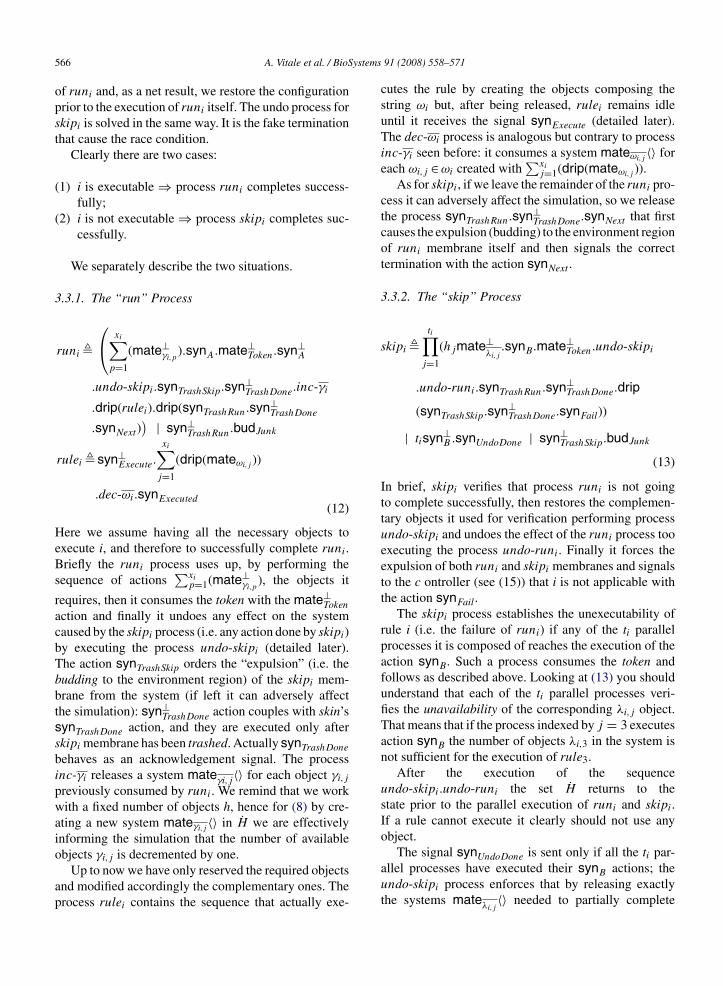
3.3.1. The “run” Process

runi �

⎛⎝

xi∑p=1

(mate⊥γi,p

).synA.mate⊥Token.syn⊥

A

.undo-skipi.synTrashSkip.syn⊥TrashDone.inc-γi

.drip(rulei).drip(synTrashRun.syn⊥TrashDone

.synNext)) | syn⊥

TrashRun.budJunk

rulei � syn⊥Execute.

xi∑j=1

(drip(mateωi,j ))

.dec-ωi.synExecuted(12)

Here we assume having all the necessary objects toexecute i, and therefore to successfully complete runi.Briefly the runi process uses up, by performing thesequence of actions

∑xip=1(mate⊥

γi,p), the objects it

requires, then it consumes the token with the mate⊥Token

action and finally it undoes any effect on the systemcaused by the skipi process (i.e. any action done by skipi)by executing the process undo-skipi (detailed later).The action synTrashSkip orders the “expulsion” (i.e. thebudding to the environment region) of the skipi mem-brane from the system (if left it can adversely affectthe simulation): syn⊥

TrashDone action couples with skin’ssynTrashDone action, and they are executed only afterskipi membrane has been trashed. Actually synTrashDone

behaves as an acknowledgement signal. The processinc-γi releases a system mateγi,j〈〉 for each object γi,j

previously consumed by runi. We remind that we workwith a fixed number of objects h, hence for (8) by cre-ating a new system mateγi,j

〈〉 in H we are effectivelyinforming the simulation that the number of available

objects γi,j is decremented by one.

Up to now we have only reserved the required objectsand modified accordingly the complementary ones. Theprocess rulei contains the sequence that actually exe-

91 (2008) 558–571

cutes the rule by creating the objects composing thestring ωi but, after being released, rulei remains idleuntil it receives the signal synExecute (detailed later).The dec-ωi process is analogous but contrary to processinc-γi seen before: it consumes a system mateωi,j

〈〉 foreach ωi,j ∈ ωi created with

∑xij=1(drip(mateωi,j )).

As for skipi, if we leave the remainder of the runi pro-cess it can adversely affect the simulation, so we releasethe process synTrashRun.syn⊥

TrashDone.synNext that firstcauses the expulsion (budding) to the environment regionof runi membrane itself and then signals the correcttermination with the action synNext .

3.3.2. The “skip” Process

skipi �ti∏

j=1

(hjmate⊥λi,j

.synB.mate⊥Token.undo-skipi

.undo-runi.synTrashRun.syn⊥TrashDone.drip

(synTrashSkip.syn⊥TrashDone.synFail))

| tisyn⊥B .synUndoDone | syn⊥

TrashSkip.budJunk

(13)

In brief, skipi verifies that process runi is not goingto complete successfully, then restores the complemen-tary objects it used for verification performing processundo-skipi and undoes the effect of the runi process tooexecuting the process undo-runi. Finally it forces theexpulsion of both runi and skipi membranes and signalsto the c ontroller (see (15)) that i is not applicable withthe action synFail.

The skipi process establishes the unexecutability ofrule i (i.e. the failure of runi) if any of the ti parallelprocesses it is composed of reaches the execution of theaction synB. Such a process consumes the token andfollows as described above. Looking at (13) you shouldunderstand that each of the ti parallel processes veri-fies the unavailability of the corresponding λi,j object.That means that if the process indexed by j = 3 executesaction synB the number of objects λi,3 in the system isnot sufficient for the execution of rule3.

After the execution of the sequenceundo-skipi.undo-runi the set H returns to thestate prior to the parallel execution of runi and skipi.If a rule cannot execute it clearly should not use anyobject.

The signal synUndoDone is sent only if all the ti par-allel processes have executed their synB actions; theundo-skipi process enforces that by releasing exactlythe systems mateλi,j

〈〉 needed to partially complete

ystems

apfoor

3P

tmnrbrtto

abopchL

onL

pcpr

A

A. Vitale et al. / BioS

ll the ti parallel processes skipi is composed of. Weoint out that only one of the ti processes will per-orm actions that follow synB since there is onlyne system mateToken〈〉 available. Moreover this willccur only if it is impossible to complete processun.

undo-runi �

⎛⎝

xi∑j=1

drip(mateγi,j )

⎞⎠ .syn⊥

A

undo-skipi�

⎛⎝

ti∑j=1

hjdrip(mateλi,j)

⎞⎠ .syn⊥

UndoDone

inc-γi �xi∑

j=1

drip(mateγi,j)

dec-ωi �xi∑

j=1

mate⊥ωi,j

token�mateToken

(14)

.4. Simulating the Non Deterministic Maximallyarallel Step

To faithfully simulate the Simple SA parallel seman-ics we must first non deterministically determine a

aximal multiset of applicable rules and then simulta-eously apply them. The number of times a particularule is executed in a specific step is not bounded,ut we recall that we can execute no more than hules at any step of computation. Given a configura-ion there may be different maximal multisets of rules,he Simple SA semantics non deterministically selectsne.

Since MDB uses a sequential semantics, we must beble to non deterministically choose up to h rules oney one. We realize this by means of systems Lv: the rolef a generic system Lvj , with 1 ≤ j ≤ h, is to select (ifossible) the jth rule and add it to the maximal set inonstruction. If system Lvj is active, then it means weave already chosen for execution j − 1 rules. Only onev system is active at a time.

Let r be the number of rules in Π. The simulationf a step of computation initiates by sending the sig-al syn1 and activating the various processes of systemv1.

When a generic Lv system activates, its controller

j

rocess sends a synStart signal that non deterministi-ally activates one of the processes that compose therocess rules. Process rules is composed by exactlyparallel processes, one for each rule of Π. Let

91 (2008) 558–571 567

i be the index of the activated process: it releasessystems runi〈〉, skipi〈〉 and token〈〉. The parallel exe-cution of these systems’ processes releases a systemrulei〈〉 (see (12)) and sends the signal synNext if rulei is executable, otherwise it sends the signal synFail.If i results executable, then we have the followingcases:

• 1 ≤ j < h: the nextj process is activated. It releasesa membrane that first causes the expulsion of theremainder of system Lvj and then activates Lvj+1by sending the signal synj+1;

• j = h: the reseth+1 process is activated. It first sendsh synExecute signal causing the execution of the h ruleprocesses that represent the maximal set of rules tobe executed, then it waits for their completion andfinally it releases a membrane that, as before, forcesthe budding of Lvj and then activates Lv1 by sendingthe signal syn1. The signal syn1 concretely starts anew step of computation.

If instead i results not executable, we have two con-ditions:

i is the r th rule we find not executable withinLvj;

B i is not the r th rule we find not executable withinLvj .

and the following cases

(1) j = 1A the simulation halts. We have zero rules

in the maximal set and no more rule tochoose;

B the controller sends another signal synStart and anew rule is evaluated;

(2) 1 < j ≤ h

A the maximal set of rules we are constructing iscomplete: j − 1synExecute signal are sent and ther ule processes are executed. After their execu-

tion, Lvj is expelled and Lv1 is activated startinga new step of computation;

B the controller sends another signal synStart and anew rule is evaluated.

ystems

568 A. Vitale et al. / BioS

The final MDB system, in its starting configuration, thatencodes the Simple SA Π is defined as follows:

Encoding� skin〈!Lv1 ◦ · · ·◦!Lvh ◦ syn1〈〉× ◦ W1 ◦ · · · ◦ Wk+1 ◦ WE ◦ O1 ◦ · · · ◦ Ok〉

where Oj stands for (mateo,j〈〉)nj , and, given multisetWj = α1, · · · , αm, Wj stands for

∏mi (mateαi,j〈〉). The

system syn1〈〉 is the one that starts the computation byactivating one of the uncountable many Lv1 systems.

4. Example: The Sodium Potassium Pump

In order to explain how the translation work, we con-sider the modeling of the so-called sodium–potassiumpump, a process which allows the exchange of sodiumand potassium ions through the cell membrane. Threesodium ions are sent, through a membrane channel, out-side the cell, by using one molecule of ATP. The channelis phosporilated and it changes its conformation to beopen to the outside. When two potassium ions enter thechannel, they are brought inside the cell, the channel isdeposhorilated, and the process is ready for a new iter-ation. Such a process can be modeled by a Simple SAsystem in the following way (we stress the fact that manydetails are ignored here):

Π = (V, μ, W1, W2, WE, R1, R2)

where:

• V = {Na,K,ATP, C}• μ = [2[1]1]2• W2 = {B, Nai|i ≥ 1}• W1 = {ATPh|h ≥ 1}• WE = {C, Kl|l ≥ 1}• R2 = {(Na3, out; C, in)} ∪ {(C, ATP, out; K2, in)}• R1 = {(B, in)} ∪ {(ATP, B, out)}

The system works in the following way.We start with a certain number i of sodium ions and a

single symbol B in region 2, with h molecules of energy

91 (2008) 558–571

(15)

ATP in region 1, with l copies of potassium ions in theenvironment, and a unique symbol C in the environment,which is used to control the whole process (one can thinkit encodes the state of the channel, defining in whichdirection it is closed).

Initially, three ions Na from region 2 are sent to theenvironment, while the symbol C is brought in region2, using the rule (Na3, out; C, in). The channel is nowopen in the direction of the environment, but it cannotbring the potassium ions inside the cell until an energyunit is available. The symbol B in region 2 is thus sent toregion 1 by the rule (B, in); here the rule (ATP, B, out)can be applied, and an energy molecule is made availablein region 2.

Using the ATP molecule in region 2, we can nowapply the rule (C, ATP, out; K2, in), which brings twoions K inside the cell. The energy unit ATP reaches theenvironment, as well as the symbol C. This last one canthus be used again to start a new cycle of the process.

We want to stress that the amount of energy in the cellis encoded in the number of symbols ATP in region 1.Each time the sodium–potassium pump is activated, oneunit of such energy is consumed (a symbol ATP reachesthe environment). When such energy units are over, theprocess cannot evolve anymore. Of course, the same istrue if less than three Na ions within the cell are availableto be sent in the environment, or less than two K ions areavailable in the environment to be brought within the cell.

4.1. Encoding the Simple SA Sodium Potassiumpump

For lack of space we do not completely detail theencoding but we present significant parts of it anddescribe the runtime scenario of the simulation. Weremember that Simple SA works with finite resourcesso we fix them in order to deal with the simplest case:

i = 3, h = 1, l = 2. This means we have |H | = h = 8(i + h + l plus a single C and a single B). With this con-ditions the model should be able to complete a singlecycle of the sodium–potassium pump.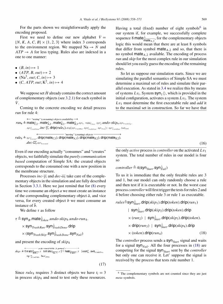

ystems

e

{tA

o

••••

oV

r

Eobct

mitovi

τ

a

Si

for a signal synFail. All the four processes in (18) arecompeting for the signal synStart sent by the controllerbut only one can receive it. Let’ suppose the signal is

A. Vitale et al. / BioS

For the parts shown we straightforwardly apply thencoding proposed.

First we need to define our new alphabet V =N, K, A, C, B} × {1, 2, 3} where index 3 correspondso the environment region. We mapped Na → N andTP → A for less typing. Rules also are indexed in ane to one manner:

(B, in) �→ 1(ATP, B, out) �→ 2(Na3, out; C, in) �→ 3(C, ATP, out; K2, in) �→ 4

We suppose set H already contains the correct amountf complementary objects (see 3.2.1) for each symbol in

˙ .Coming to the concrete encoding we detail process

un for rule 4:

ven if our encoding actually “consumes” and “creates”bjects, we faithfully simulate the purely communicationased computation of Simple SA: the created objectsorresponds to the consumed one with a new position inhe membrane structure.

Processes inc-γi and dec-ωi take care of the comple-entary objects in the simulation and are fully described

n Section 3.3.1. Here we just remind that for (8) everyime we consume an object a we must create an instancef the corresponding complementary object a, and viceersa, for every created object b we must consume annstance of b.

We define τ as follow

� synB.mate⊥Token.undo-skip4.undo-run4.

× synTrashRun.syn⊥TrashDone.drip

× (synTrashSkip.syn⊥TrashDone.synFail)

nd present the encoding of skip4

(17)

ince rule4 requires 3 distinct objects we have ti = 3n process skip4 and need to test only these resources.

91 (2008) 558–571 569

(16)

Having a total (fixed) number of eight symbols6 inour system if, for example, we successfully completesequence 8 mate⊥

mateA,2, for the complementary objects

logic this would mean that there are at least 8 symbolsthat differ from symbol mateA,2 and so, that there isno symbol mateA,2 available. The encoding of processrun and skip for the most complex rule in our simulationshould let you easily guess the encoding of the remainingrules.

So let us suppose our simulation starts. Since we aresimulating the parallel semantics of Simple SA we mustdetermine a maximal set of rules and simulate their par-allel execution. As stated in 3.4 we realize this by meansof systems Lvi. System syn1〈〉, which is provided in theinitial configuration, activates a system Lv1. The systemLv1 must determine the first executable rule and add itto the maximal set in construction. So far we have that

the only active process is controller on the activated Lv1system. The total number of rules in our model is fourso

controller� 4(synStart .syn⊥Fail)

To us it is immediate that the only fireable rules are 3and 1, but our model can only randomly choose a ruleand then test if it is executable or not. In the worst caseprocess controller will first trigger the tests for rules 2 and4 before choosing either rule 3 or rule 1 as executable.

rules�syn⊥Start .drip(skip1).drip(token).drip(run1)

| syn⊥Start .drip(skip2).drip(token).drip

× (run2) | syn⊥Start .drip(skip3).drip(token).

× drip(run3) | syn⊥Start .drip(skip4).drip

× (token).drip(run4) (18)

The controller process sends a synStart signal and waits

received by the process that tests rule number 1.

6 The complementary symbols are not counted since they are justmeta–symbols.

ystems

We recall here that, as pointed out in the previous sec-

570 A. Vitale et al. / BioS

The testing of rule 1 starts by releasing the sys-tems skip1〈〉, run1〈〉 and token〈〉. Since we have anobject B in region 2, rule 1 is executable: processrun1 releases the system rule1〈〉. Please note that pro-cess rule1 will execute only after receiving a signalsynExecute. The remainder of system run1〈〉 is expelledout to the environment and the signal synNext isproduced.

So far system Lv1 has accomplished its goal byadding rule 1 to the maximal set we are constructing.The signal synNext is received by the process next1 onsystem Lv1, the remainder of system Lv1 is expelled tothe environment and the signal syn2 is produced. Thisactivates a system Lv2 which goal is to find anotherexecutable rule. We want to stress out that we have notyet executed process rule1, it is still awaiting for a sig-nal synExecute, but we have indeed locked resources forits execution. Clearly the locked resources will not beavailable to system Lv2.

System Lv2 undergoes, more or less, the samesequence we just described for system Lv1. Briefly, anew system rule3〈〉 is released, the remainder of systemLv2 is discarded to the environment and a signal syn3 isproduced.

It should be easy too see no more rules are executable.System Lv3 will indeed test all the four rules of our simu-lation but no runi process is going to succeed. Every testwill indeed terminate by sending a synFail signal. Sincefour synFail signals are produced the controller processwill complete its sequence and so the signal synReset willbe produced (see (15)). The signal produced triggers thereset3 process on system Lv3.

So far our simulation have completed the maximalset of rules (with rules 1 and 3), and now we must exe-cute the chosen rules and start a new step of computa-tion.

It is the reset3 process that triggers the execution ofprocesses rule1 and rule3 by producing two synExecute

signals. After the execution, processes rule1 and rule3reply with one synExecuted signal each. The reset3 pro-cess receives the two signals and forces the expulsion tothe environment of the remainder of system Lv3. Finally,it produces a new syn1 signal. As you can easily see theproduced signal triggers a new Lv1 system and a newstep of computation starts.

At this point we have successfully simulated the paral-lel execution of rules 1 and 3 by simulating the transportof a B symbol from region 2 to region 1, the transport ofthree N symbols from region 2 to the environment and

the transport of a single C symbol from the environmentto region 2. To simulate this we deleted the symbols

mateB,2, 3mateN,2, mateC,3

91 (2008) 558–571

and produced the following

mateB,1, 3mateN,3, mateC,2

We chose some “lucky” branch in our simulation inorder to avoid the description of a long and tedious skipprocess, but you should note that, given the starting con-figuration, in whichever order we test our rules we obtaina maximal set containing exactly rules 3 an 1 since it isthe unique maximal set possible.

The simulation undergoes two more computation stepexecuting rule 2 in the first step and rule 4 in parallel withrule 1 in the second one. After completing this last stepthe simulation will start a new step searching for a newexecutable rule by means of a system Lv1. Since we can-not execute any rules four synFail signals are produced,the controller process on Lv1 completes and, with noactive process, the entire simulation stops (see definitionof Lv1 in (15)).

A single cycle of the sodium–potassium pump hasbeen simulated.

5. Conclusion and Final Remarks

This paper is a contribution to the recently startedinvestigations aiming to bridge two research areas whichare both inspired by the functioning of the living cell:Membrane computing and Brane calculi.

We have presented a simulation of a variant of Mem-brane systems by means of Brane calculi based onthe three operations Mate/Bud/Drip. As the main ideabehind the paper was to investigate the use of these twoframeworks in Systems Biology area, we chose to startfrom simple formalisms: we chose MBD Brane calculus,which is non-Turing equivalent, to simulate a variant of Psystems called Simple symport/antiport P systems (Sim-ple SA); the computations of this last type of systems is,in fact, purely based on communications of objects and itis obtained by coupling chemicals and by changing theirposition with respect to the compartments defined by themembrane structure used, and not by creating or destroy-ing some of them. Their behaviour is thus closely relatedto the biological trans-membrane communication, andthey can be effectively used in describing such processes.Moreover, compared with basic symport/antiport P sys-tems, Simple SA is a less powerful computational device,but its limited resources scenario makes it a more realisticmodel for System Biology.

tion, the encoding we have proposed is non deterministic:if the Simple SA system to be simulated is non determin-istic, then also the MDB encoding is non deterministic.

ystems

InM

ibcoot

A

M0(

h

R

B

B

C

on membranes. In: Proceedings of the Third Brainstorming Week

A. Vitale et al. / BioS

t remains an open problem to show if it is possible orot to simulate Simple SA systems using deterministicBD Brane calculus.Many other related research topics remains to be

nvestigated: the simulation of other classes of P systemsy means of MBD Brane calculus, the use of Brane cal-ulus using the Pino/Exo/Phago operations, and the usef different types of parallelisms within the frameworkf Brane calculi are the directions we plan to explore inhe near future.

cknowledgements

This work has been partially supported by the Italianinistry of University (MIUR) under the project PRIN-

4 “Systems Biology: modellazione, linguaggi e analisiSYBILLA)”.

Finally, we thank the anonymous reviewers for theirelpful comments and suggestions.

eferences

usi, N., 2005. On the computational power of the mate/bud/drip Branecalculus: interleaving vs. maximal parallelism. In: Pre-Proc. ofSixth International Workshop on Membrane Computing (WMC6),Vienna, June 18–21, 2005, pp. 235–252.

usi, N., Gorrieri, R., 2005. On the computational power of Branecalculi. In: CMSB 2005, pp. 106–117.

ardelli, L., 2004. Brane calculi: interactions of biological membranes.In: Danos, V., Schachter, V. (Eds.), CMSB, vol. 3082 of LectureNotes in Computer Science, Springer, pp. 257–278.

91 (2008) 558–571 571

Cardelli, L., Paun, G., 2005. An universality result for a (mem)branecalculus based on mate/drip operations. In: Proceedings ofthe ESF Exploratory Workshop on Cellular Computing (Com-plexity Aspects), Sevilla (Spain), January 31–February 2, pp.75–94.

Ginsburg, S., 1966. The Mathematical Theory of Context. Free Lan-guages. McGraw-Hill, New York.

Ibarra, O.H., Woodworth, S., Yen, H.-C., Dang, Z. On symport/antiportsystems and semilinear sets. In: Proceedings of the 6th Inter-national Workshop on Membrane Computing (WMC6), 2005.Lecture Notes in Computer Science, Springer, pp. 312–335, inpress.

Paun, A., Paun, G., May 2002. The power of communication: P Sys-tems with symport/antiport. New Gen. Comput. 20 (3), 295–305.

Paun, G., 1998. Computing with membranes. Technical Report 208,Turku Center for Computer Science-TUCS. (www.tucs.fi).

Paun, G., February 1999. Computing with membranes. An introduc-tion. Bull. EATCS (67), 139–152.

Paun, G., 2002. Membrane Computing. An Introduction. Springer-Verlag, Berlin.

Paun, G., 2003. Membrane computing. In: Lingas, A., Nilsson, B.J.(Eds.), Fundamentals of Computation Theory 14th InternationalSymposium, FCT 2003. Malmo, Sweden, August 12–15, 2003.Proceedings. volume 2751 of Lecture Notes in Computer Science,pp. 284–295. Springer, 2003.

Paun, G., 2004. Introduction to membrane computing. In: First Brain-storming Workshop on Uncertainty in Membrane Computing,Palma de Mallorca, Spain, November 2004.

Paun, G., 2005. One more universality result for P systems with objects

on Membrane Computing, Sevilla (Spain), January 31–February4, pp. 263–274.

Rozenberg, G., Salomaa, A., 1997. Handbook of Formal Language,vols I–III. Springer Verlag, Berlin Heidelberg.