
Bounded model checking for asynchronous concurrent systems.
172
Bounded Model Checking for Asynchronous Concurrent Systems Manitra Johanesa Rakotoarisoa Department of Computer Architecture Technical University of Catalonia Advisor: Enric Pastor Llorens Thesis submitted to obtain the qualification of Doctor from the Technical University of Catalonia
Transcript of Bounded model checking for asynchronous concurrent systems.

Bounded Model Checking forAsynchronous Concurrent
Systems
Manitra Johanesa RakotoarisoaDepartment of Computer Architecture
Technical University of Catalonia
Advisor: Enric Pastor Llorens
Thesis submitted to obtain the qualification of Doctorfrom the Technical University of Catalonia


To my mother


Contents
Abstract xvii
Acknowledgments xix
1 Introduction 11.1 Symbolic Model Checking . . . . . . . . . . . . . . . . . . . . . . . . . . . 3
1.1.1 BDD-based approach . . . . . . . . . . . . . . . . . . . . . . . . . . 31.1.2 SAT-based Approach . . . . . . . . . . . . . . . . . . . . . . . . . . 6
1.2 Synchronous Versus Asynchronous Systems . . . . . . . . . . . . . . . . . 81.2.1 Synchronous systems . . . . . . . . . . . . . . . . . . . . . . . . . . 81.2.2 Asynchronous systems . . . . . . . . . . . . . . . . . . . . . . . . . 10
1.3 Scope of This Work . . . . . . . . . . . . . . . . . . . . . . . . . . . . . . 111.4 Structure of the Thesis . . . . . . . . . . . . . . . . . . . . . . . . . . . . . 12
2 Background 132.1 Transition Systems . . . . . . . . . . . . . . . . . . . . . . . . . . . . . . . 13
2.1.1 Definitions . . . . . . . . . . . . . . . . . . . . . . . . . . . . . . . 132.1.2 Symbolic Representation . . . . . . . . . . . . . . . . . . . . . . . . 15
2.2 Other Models for Concurrent Systems . . . . . . . . . . . . . . . . . . . . 172.2.1 Kripke Structure . . . . . . . . . . . . . . . . . . . . . . . . . . . . 172.2.2 Petri Nets . . . . . . . . . . . . . . . . . . . . . . . . . . . . . . . . 212.2.3 Automata . . . . . . . . . . . . . . . . . . . . . . . . . . . . . . . . 22
2.3 Linear Temporal Logic . . . . . . . . . . . . . . . . . . . . . . . . . . . . . 242.4 Satisfiability Problem . . . . . . . . . . . . . . . . . . . . . . . . . . . . . 26
2.4.1 DPLL Algorithm . . . . . . . . . . . . . . . . . . . . . . . . . . . . 272.4.2 Stålmarck’s Algorithm . . . . . . . . . . . . . . . . . . . . . . . . . 282.4.3 Other Methods for Solving SAT . . . . . . . . . . . . . . . . . . . 32
2.5 Bounded Model Checking . . . . . . . . . . . . . . . . . . . . . . . . . . . 342.5.1 BMC Idea . . . . . . . . . . . . . . . . . . . . . . . . . . . . . . . . 342.5.2 Safety Check Example . . . . . . . . . . . . . . . . . . . . . . . . . 342.5.3 BMC and Liveness Properties . . . . . . . . . . . . . . . . . . . . . 35
vi CONTENTS
3 Exixting Techniques 373.1 Standard Methods . . . . . . . . . . . . . . . . . . . . . . . . . . . . . . . 373.2 Completeness . . . . . . . . . . . . . . . . . . . . . . . . . . . . . . . . . . 393.3 SAT with Unbounded Model Checking . . . . . . . . . . . . . . . . . . . . 413.4 Existing BMC Tools . . . . . . . . . . . . . . . . . . . . . . . . . . . . . . 42
4 Encoding Methods 434.1 Related Work . . . . . . . . . . . . . . . . . . . . . . . . . . . . . . . . . . 444.2 Symbolic Representation . . . . . . . . . . . . . . . . . . . . . . . . . . . . 454.3 Encoding for Independent Systems . . . . . . . . . . . . . . . . . . . . . . 46
4.3.1 Interleaving Execution . . . . . . . . . . . . . . . . . . . . . . . . . 464.3.2 Breadth-First Search Execution . . . . . . . . . . . . . . . . . . . . 48
4.4 Encoding for Synchronized Systems . . . . . . . . . . . . . . . . . . . . . . 514.4.1 Interleaving Execution . . . . . . . . . . . . . . . . . . . . . . . . . 514.4.2 Breadth-First Search Execution . . . . . . . . . . . . . . . . . . . . 54
4.5 Expressing Reachability Properties . . . . . . . . . . . . . . . . . . . . . . 564.6 Reducing the Bound Using Chaining . . . . . . . . . . . . . . . . . . . . . 58
4.6.1 Introduction . . . . . . . . . . . . . . . . . . . . . . . . . . . . . . 584.6.2 Application to BMC . . . . . . . . . . . . . . . . . . . . . . . . . . 594.6.3 Ordering the Events . . . . . . . . . . . . . . . . . . . . . . . . . . 614.6.4 Chaining Algorithm . . . . . . . . . . . . . . . . . . . . . . . . . . 63
5 Leap-Based Approach 655.1 Related Work . . . . . . . . . . . . . . . . . . . . . . . . . . . . . . . . . . 665.2 Unrolling Method for Deadlock Property . . . . . . . . . . . . . . . . . . . 67
5.2.1 Introduction . . . . . . . . . . . . . . . . . . . . . . . . . . . . . . 675.2.2 BMC Equations . . . . . . . . . . . . . . . . . . . . . . . . . . . . 68
5.3 Unrolling Method for Other Reachability Properties . . . . . . . . . . . . 705.3.1 Introduction . . . . . . . . . . . . . . . . . . . . . . . . . . . . . . 705.3.2 BMC Equations . . . . . . . . . . . . . . . . . . . . . . . . . . . . 71
5.4 Jumping Methods . . . . . . . . . . . . . . . . . . . . . . . . . . . . . . . 735.4.1 Using Logarithmic Functions . . . . . . . . . . . . . . . . . . . . . 735.4.2 Using Interpolation . . . . . . . . . . . . . . . . . . . . . . . . . . . 76
5.5 Finding the Shortest Counterexample . . . . . . . . . . . . . . . . . . . . 775.6 Time Performance . . . . . . . . . . . . . . . . . . . . . . . . . . . . . . . 77
6 An Automata-Theoretic Approach 816.1 Related Work . . . . . . . . . . . . . . . . . . . . . . . . . . . . . . . . . . 836.2 Representation of Büchi Automata . . . . . . . . . . . . . . . . . . . . . . 84
6.2.1 Different Types of Büchi Automata . . . . . . . . . . . . . . . . . . 846.2.2 Translating an LTL Formula Into a TGBA . . . . . . . . . . . . . . 866.2.3 TGBA Encoding . . . . . . . . . . . . . . . . . . . . . . . . . . . . 90
CONTENTS vii
6.3 Building the BMC Formulas . . . . . . . . . . . . . . . . . . . . . . . . . . 926.3.1 Interleaving Execution . . . . . . . . . . . . . . . . . . . . . . . . . 926.3.2 Breadth First Search Execution . . . . . . . . . . . . . . . . . . . . 946.3.3 Chaining . . . . . . . . . . . . . . . . . . . . . . . . . . . . . . . . 96
6.4 Discussion . . . . . . . . . . . . . . . . . . . . . . . . . . . . . . . . . . . . 97
7 Implementation 997.1 Different Modules . . . . . . . . . . . . . . . . . . . . . . . . . . . . . . . . 99
7.1.1 LTL2BA . . . . . . . . . . . . . . . . . . . . . . . . . . . . . . . . . 997.1.2 BMC Module . . . . . . . . . . . . . . . . . . . . . . . . . . . . . . 1017.1.3 CNF translator . . . . . . . . . . . . . . . . . . . . . . . . . . . . . 1037.1.4 Solver . . . . . . . . . . . . . . . . . . . . . . . . . . . . . . . . . . 103
7.2 Input Formats . . . . . . . . . . . . . . . . . . . . . . . . . . . . . . . . . 1047.2.1 TS File format . . . . . . . . . . . . . . . . . . . . . . . . . . . . . 1047.2.2 PEP File format . . . . . . . . . . . . . . . . . . . . . . . . . . . . 105
7.3 Important commands . . . . . . . . . . . . . . . . . . . . . . . . . . . . . 107
8 Case Studies 1118.1 Experiments Related to Reachability . . . . . . . . . . . . . . . . . . . . . 111
8.1.1 Explication of the Benchmarks . . . . . . . . . . . . . . . . . . . . 1128.1.2 Comparison with the Tool NuSMV . . . . . . . . . . . . . . . . . . 113
8.2 Experimental Results Related to LTL . . . . . . . . . . . . . . . . . . . . 1148.2.1 Gas Station . . . . . . . . . . . . . . . . . . . . . . . . . . . . . . . 1148.2.2 Bakery Algorithm . . . . . . . . . . . . . . . . . . . . . . . . . . . 1148.2.3 Readers-writers Problem . . . . . . . . . . . . . . . . . . . . . . . . 1148.2.4 Sleeping Barber . . . . . . . . . . . . . . . . . . . . . . . . . . . . . 1158.2.5 Leader Election Protocol . . . . . . . . . . . . . . . . . . . . . . . 1158.2.6 Properties and Instances . . . . . . . . . . . . . . . . . . . . . . . . 115
8.3 Experiments Related to Leap . . . . . . . . . . . . . . . . . . . . . . . . . 1178.4 Example of a Leap Execution . . . . . . . . . . . . . . . . . . . . . . . . . 118
9 Conclusions and Future Work 1219.1 Conclusions . . . . . . . . . . . . . . . . . . . . . . . . . . . . . . . . . . . 1219.2 Future Work . . . . . . . . . . . . . . . . . . . . . . . . . . . . . . . . . . 122
Bibliography 123
Index 151

List of Figures
1.1 Model Checking. . . . . . . . . . . . . . . . . . . . . . . . . . . . . . . . . 21.2 Image computation. . . . . . . . . . . . . . . . . . . . . . . . . . . . . . . 3
2.1 A Transition system. . . . . . . . . . . . . . . . . . . . . . . . . . . . . . . 142.2 To and From sets. . . . . . . . . . . . . . . . . . . . . . . . . . . . . . . . 152.3 Different ways for representing the states. . . . . . . . . . . . . . . . . . . 182.4 A Kripke structure model of a simple traffic light controller. . . . . . . . . 192.5 Runs from the traffic light controller. . . . . . . . . . . . . . . . . . . . . . 202.6 Computation tree of the traffic light controller. . . . . . . . . . . . . . . . 202.7 A Petri net version of the traffic light controller. . . . . . . . . . . . . . . 222.8 An automaton model of a digicode. . . . . . . . . . . . . . . . . . . . . . . 242.9 A two bit counter. . . . . . . . . . . . . . . . . . . . . . . . . . . . . . . . 34
4.1 A Transition system. . . . . . . . . . . . . . . . . . . . . . . . . . . . . . . 454.2 Interleaving (1) vs. BFS. (2) . . . . . . . . . . . . . . . . . . . . . . . . . 484.3 Synchronized product of TSs. . . . . . . . . . . . . . . . . . . . . . . . . . 534.4 Typical BFS execution for synchronized systems. . . . . . . . . . . . . . . 564.5 Chaining execution with event order [a, c, b, d]. . . . . . . . . . . . . . . . 594.6 Chaining execution for synchronized systems. . . . . . . . . . . . . . . . . 604.7 BFS with chaining using two different event orders. . . . . . . . . . . . . . 61
5.1 Unrolling using leaps. . . . . . . . . . . . . . . . . . . . . . . . . . . . . . 665.2 A synchronized system with idle steps. . . . . . . . . . . . . . . . . . . . . 675.3 Leap methods for deadlock property. . . . . . . . . . . . . . . . . . . . . . 705.4 Leap methods for other reachability properties. . . . . . . . . . . . . . . . 725.5 Different leap values. . . . . . . . . . . . . . . . . . . . . . . . . . . . . . . 745.6 Plot for the base 2 logarithmic function. . . . . . . . . . . . . . . . . . . . 745.7 The interpolation method with the collected points. . . . . . . . . . . . . 77
6.1 Automata-theoretic approach to BMC. . . . . . . . . . . . . . . . . . . . . 826.2 A Büchi automaton. . . . . . . . . . . . . . . . . . . . . . . . . . . . . . . 856.3 A Transition-based Büchi automaton. . . . . . . . . . . . . . . . . . . . . 86

x LIST OF FIGURES
6.4 TGBA for the LTL formula (Fa^ F a). . . . . . . . . . . . . . . . . . . . 886.5 TGBA for the LTL formula φ a R pc_ bq. . . . . . . . . . . . . . . . . . 916.6 A complete example: two TSs and a TGBA. . . . . . . . . . . . . . . . . . 93
7.1 BMC++ major modules. . . . . . . . . . . . . . . . . . . . . . . . . . . . 1007.2 The tree representation of the LTL formula Fa^ F a. . . . . . . . . . . . 1017.3 Details of the LTL2BA Module (1), and the BMC Module (2). . . . . . . 1027.4 A transition system. . . . . . . . . . . . . . . . . . . . . . . . . . . . . . . 1037.5 A Petri net. . . . . . . . . . . . . . . . . . . . . . . . . . . . . . . . . . . . 107

List of Tables
2.1 Typical CNF Translation for the gates AND, OR, and NOT . . . . . . . . 33
6.1 Tableau Rules . . . . . . . . . . . . . . . . . . . . . . . . . . . . . . . . . . 87
7.1 LTL operators and their keyboard equivalents . . . . . . . . . . . . . . . . 100
8.1 Deadlock detection results . . . . . . . . . . . . . . . . . . . . . . . . . . . 1128.2 Comparison with NuSMV . . . . . . . . . . . . . . . . . . . . . . . . . . . 1138.3 LTL checking results . . . . . . . . . . . . . . . . . . . . . . . . . . . . . . 1168.4 Comparison of leap and standard BMC . . . . . . . . . . . . . . . . . . . 117

List of Algorithms
1.1 forwardReachability . . . . . . . . . . . . . . . . . . . . . . . . . . . . . . . 41.2 standardBmcAlgorithm . . . . . . . . . . . . . . . . . . . . . . . . . . . . . 72.1 dpll . . . . . . . . . . . . . . . . . . . . . . . . . . . . . . . . . . . . . . . . 282.2 zeroSaturate . . . . . . . . . . . . . . . . . . . . . . . . . . . . . . . . . . . 312.3 saturate . . . . . . . . . . . . . . . . . . . . . . . . . . . . . . . . . . . . . . 324.1 Bmc . . . . . . . . . . . . . . . . . . . . . . . . . . . . . . . . . . . . . . . . 635.1 JumpByLogarithm . . . . . . . . . . . . . . . . . . . . . . . . . . . . . . . . 755.2 jumpByInterpolation . . . . . . . . . . . . . . . . . . . . . . . . . . . . . . 76

Nomenclature
BA Büchi automata
BDD Binary decision diagrams
BMC Bounded model checking
CAD Computer-aided design
CNF Conjunctive normal form
CTL Computation tree logic
DPLL Davis-Putnam-Longeman-Loveland, name of an algorithm for solving SAT
FSM Finite state machine
LTL Linear temporal logic
NuSmv A model checking tool that has BMC capabilities
PN Petri net
SAT Boolean satisfiability problem
TGBA Transition-based generalized Büchi automata
TS Transition system
ZChaff A SAT solver

Abstract
In this thesis we study the verification of asynchronous concurrent systems using a sym-bolic model checking technique called bounded model checking (BMC). BMC is a methodtargeted mainly at finding bugs in a system. It answers the question whether there existsan execution path, shorter than a given number, that violates a given property. Such anexecution path is known as counterexample. During a BMC operation each execution pathis encoded into a Boolean formula, and the problem is reduced to satisfiability checking ofthe formula. Therefore, the operation consists mainly in constructing a Boolean formulathat is satisfiable if and only if such a counterexample exists.
We model our systems with transition systems (TSs). In particular, we are mainlyinterested in synchronized product of TSs. Since concurrent systems are formed by a com-bination of several components communicating between each other, synchronized productof TSs is well-suited to capture the behavior of such systems. The executions of con-current systems are commonly modeled using the so-called interleaving execution, whichallows only one single event to fire at each step. However, due to the complexity of suchsystems, performing BMC with interleaving will not only require many steps but alsogenerate long formulas. In this work, we adopt different approaches based on breadth-firstsearch (BFS). Our methods reduce the necessary steps, and produce smaller formulas. Ina BMC operation, the translation of the model into a Boolean formula is polynomial inthe size of the model, but the solving time of the Boolean formula can be exponentialin the size of the formula. Therefore, our research hypothesis is that we can improvethe efficiency of BMC by generating succinct formula, and by minimizing the number ofnecessary steps during an execution.
We introduce several BMC techniques aimed at improving the efficiency of BMC forasynchronous concurrent systems. The techniques are grouped in two main parts (i) tech-niques for checking reachability properties and (ii) techniques for checking other proper-ties written in linear temporal logic (LTL). In addition, we also propose some methods forminimizing the number of execution steps or bounds.
We implemented all these methods in a BMC toolset. At the end of the dissertation,we will discuss the experimental results we obtained.
Keywords: bounded model checking, asynchronous concurrent systems, satisfiabilityproblem, reachability properties, linear temporal logic.


Acknowledgments
This thesis would not have been possible without the support of many people. It is apleasure for me to thank all of them.
First, I would like to express my sincere gratitude to my supervisor Enric Pastor whooffered invaluable assistance, support, and guidance throughout my work. With his greatefforts to explain things clearly and simply, he helped make formal verification fun forme. He also provided encouragement and good company. I would have been lost withouthim.
I am indebted to all my colleagues at the Computer Architecture Department forproviding a stimulating and pleasant working environment. Especially, I am grateful toMarc Solé, Josep Carmona, and Juan Lopez who spent a great deal of their time discussingwith me, and gave sound advice that contributed in many ways to the accomplishment ofthis research project.
Special thanks to the external reviewers, Marco Peña and Robert Viladrosa who care-fully read the preliminary version of this report and provided valuable suggestions andcomments. Thanks also to all the members of the jury for evaluating and judging mythesis.
I would like to show my gratitude to the following institutions for funding this research:the Government of Catalonia under the scholarship FI, and the Ministry of Science andEducation of Spain under the contract CICYT TIN 2007-63927.
I wish to thank all my friends, especially Nirina Rakotoarivelo, Rafael Ordonez, Man-itra Raharijaona, and Fidel Pedregal Pimentel. They encouraged me and supported mefrom the beginning until the end, despite the long period of time I spent doing my Ph.D.thesis.
I would also like to thank my entire family for their unwavering support. Most impor-tantly, I am very thankful to my mother, Marguerite Ravaoarivelo. She bore me, raisedme, taught me, and has loved me throughout the years. To her I dedicate this thesis.
Last but not least, I would like to express my gratitude to all the people who havenot been cited above but who helped me directly or indirectly with the realization of thisthesis. Thank you so much everyone.

Chapter 1
Introduction
Complex hardware systems become more and more ubiquitous in mission critical appli-cations such as military, satellite, and medical to name but a few. In such applications,reliability remains a primary concern because a failure that occurs during their normal op-erations might produce important catastrophes like loss of life or loss of money. Examplesof these catastrophes include the Pentium bug [Gep95, Ade97], space launch disasters likethe Mariner I [HL05] or the Ariane 5 [Har03], the Warsaw A320 crash [Lad95, CMMM95],not to mention the AT&T telephone switching failure [Ste93, Har00].
All these failures are often caused by minuscule bug1 that exists inside the softwarewhich controls the systems, or within the hardware itself. In addition, most of thesesystems cannot be interrupted while working, even for a few seconds a year, making itdifficult to repair bugs found during their normal operations.
Therefore, manufacturers of such systems have to validate their designs, before ship-ping them to ward off disasters caused by undetected errors. Appropriate validationtechniques are then necessary to discover bugs that would affect the use of such systems.
In general, design validation can be performed using two groups of methods: (i) sim-ulation and testing (ii) formal verification.
In simulation and testing, the main purpose is to carry out some experiments beforegetting the product on the market. This involves introducing series of inputs into thedesign and checking whether the produced outputs correspond to the expected ones.Simulation and testing explore only some system behaviors and they take time to find theslightest bugs in a system. Hence, they can overlook considerable errors if the system has
1Bug is a computer jargon referring to an undesirable property that makes the computer misbehaveor crash. The first recorded bug was a real insect. In 1947, American mathematician and computerscientist Grace Murray Hopper (1906-1992), known also for inventing the programming language COBOL,was working on the Harvard University’s Mark II computer. One day, the machine crashed. Hopperinvestigated and found that a moth has squeezed into one of the 17,000 relays in the machine. Sheremoved the moth and the machine worked perfectly [Kid98, Nor05]. This is not, however the origin ofthe term “bug” since this term has already been used long before by other scientists, but Hopper’s wasthe “first actual case of a bug being found” according to a note she put on her log book.
2 Introduction
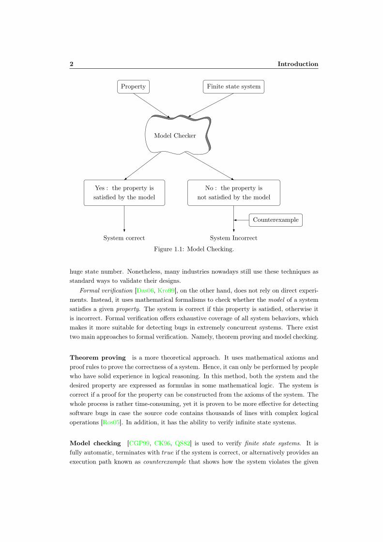
Property Finite state system
Model Checker
Yes : the property is
satisfied by the model
No : the property is
not satisfied by the model
Counterexample
System correct System Incorrect
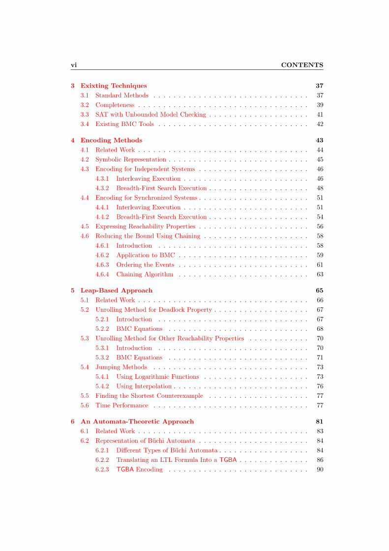
Figure 1.1: Model Checking.
huge state number. Nonetheless, many industries nowadays still use these techniques asstandard ways to validate their designs.
Formal verification [Das06, Kro99], on the other hand, does not rely on direct experi-ments. Instead, it uses mathematical formalisms to check whether the model of a systemsatisfies a given property. The system is correct if this property is satisfied, otherwise itis incorrect. Formal verification offers exhaustive coverage of all system behaviors, whichmakes it more suitable for detecting bugs in extremely concurrent systems. There existtwo main approaches to formal verification. Namely, theorem proving and model checking.
Theorem proving is a more theoretical approach. It uses mathematical axioms andproof rules to prove the correctness of a system. Hence, it can only be performed by peoplewho have solid experience in logical reasoning. In this method, both the system and thedesired property are expressed as formulas in some mathematical logic. The system iscorrect if a proof for the property can be constructed from the axioms of the system. Thewhole process is rather time-consuming, yet it is proven to be more effective for detectingsoftware bugs in case the source code contains thousands of lines with complex logicaloperations [Ros05]. In addition, it has the ability to verify infinite state systems.
Model checking [CGP99, CK96, QS82] is used to verify finite state systems. It isfully automatic, terminates with true if the system is correct, or alternatively provides anexecution path known as counterexample that shows how the system violates the given
1.1. Symbolic Model Checking 3
S0 S1 S2. . . Sk
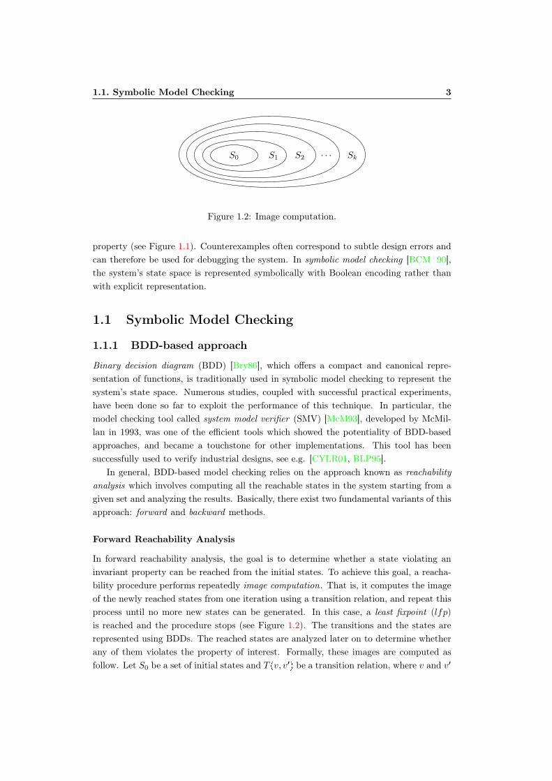
Figure 1.2: Image computation.
property (see Figure 1.1). Counterexamples often correspond to subtle design errors andcan therefore be used for debugging the system. In symbolic model checking [BCM90],the system’s state space is represented symbolically with Boolean encoding rather thanwith explicit representation.
1.1 Symbolic Model Checking
1.1.1 BDD-based approach
Binary decision diagram (BDD) [Bry86], which offers a compact and canonical repre-sentation of functions, is traditionally used in symbolic model checking to represent thesystem’s state space. Numerous studies, coupled with successful practical experiments,have been done so far to exploit the performance of this technique. In particular, themodel checking tool called system model verifier (SMV) [McM93], developed by McMil-lan in 1993, was one of the efficient tools which showed the potentiality of BDD-basedapproaches, and became a touchstone for other implementations. This tool has beensuccessfully used to verify industrial designs, see e.g. [CYLR01, BLP95].
In general, BDD-based model checking relies on the approach known as reachabilityanalysis which involves computing all the reachable states in the system starting from agiven set and analyzing the results. Basically, there exist two fundamental variants of thisapproach: forward and backward methods.
Forward Reachability Analysis
In forward reachability analysis, the goal is to determine whether a state violating aninvariant property can be reached from the initial states. To achieve this goal, a reacha-bility procedure performs repeatedly image computation. That is, it computes the imageof the newly reached states from one iteration using a transition relation, and repeat thisprocess until no more new states can be generated. In this case, a least fixpoint (lfp)is reached and the procedure stops (see Figure 1.2). The transitions and the states arerepresented using BDDs. The reached states are analyzed later on to determine whetherany of them violates the property of interest. Formally, these images are computed asfollow. Let S0 be a set of initial states and T pv, v1q be a transition relation, where v and v1

4 Introduction
denotes the current and next state variables respectively. Let us use Spvq and T pv, v1q todenote the propositional formulas related to the set of states and transitions respectively.Then, the image of Spvq through T pv, v1q is given as:
ImgpSpv1qq Dv.T pv, v1q ^ Spvq (1.1)
Now, starting from the initial states, the least fixed point can be computed by repeat-edly applying the following equation in which the final results of the set R contains allforward reached states:
R lfp R.pS0 _ ImgpRqq (1.2)
For instance, assume we want to check whether a system satisfies a safety propertyexpressing that something should be true at every state of the system. In this case, themodel checker applies repeatedly image computation to determine if there is an executionpath from an initial state to a state where this property fails. If such a path does notexist, then the system is correct, otherwise the system is incorrect and the path found bythe model checker corresponds to a counterexample.
Algorithm 1.1 illustrates the forward reachability procedure. The set R contains allreachable states, while Si contains the newly discovered states in each iteration. Thefunction img() perform the image computation from Si. The algorithm stops when Si isempty.
Algorithm 1.1: forwardReachabilityinput : S0 a set of initial statesoutput: R a set of reachable states
RÐÝ H ;1
iÐÝ 0 ;2
while (Si H) do3
RÐÝ RY Si ;4
Si1 ÐÝ img(Si) zR ;5
iÐÝ i 1 ;6
end7
return R8
Note that, for large systems, the final set R may become too big. To avoid thissituation, some people perform on-the-fly check of the invariant property. That is, at eachiteration the newly reached states is checked whether any of them violates the property.If the answer is positive, then the algorithm stops. This method prevents explorationthrough the entire state space.
1.1. Symbolic Model Checking 5
Backward Reachability Analysis
Backward reachability is mainly used to perform diagnostic of a failure in a system.As its name suggests, it is the opposite of forward reachability. The aim in here is toknow whether a specified set of target (i.e violating) states is reachable from any of theinitial states. To do so, the procedure starts from the set of violating states and performpreimage computation repeatedly until a fixpoint is reached. Then, it checks if the reachedset contains one of the initial states. As before, all states and transitions are encodedwith BDDs. Formally a preimage computation is performed as follow. Let T pv.v1q be atransition relation and St a set of target states. The preimage of Spv1q through T pv, v1qis given as:
PreImgpSpvqq Dv1.T pv, v1q ^ Spv1q (1.3)
and the least fixed point is obtained by repeatedly applying the following equation fromthe target set:
R lfp R.pSt _ PreImgpRqq (1.4)
The algorithm for backward reachability is similar to Algorithm 1.1. We need onlyto start from St instead of S0. On-the-fly methods can also be applied to backwardreachability in order to handle large systems.
State Explosion Problem
Although successful, BDD-based approaches are subject to the so-called state explosionproblem, or the situation where the size of the state space grows exponentially beyondthe available computer resources. This situation arises if the system being checked hasmany components that can make transitions in parallel. For that reason, certain types ofdesigns cannot be handled efficiently with BDD-based approaches. Below, we will reviewbriefly some interesting techniques for dealing with the state explosion problem. Namely,partial order reduction, compositional reasoning, abstraction, induction, and symmetry.
Partial Order Reduction This technique is designed for concurrent systems withcommunicating processes [GW94, Pel93, WW96, NG02]. With this technique, when con-current events are independent, it suffices to consider one of them since, in this case, theyall lead to the same state. Therefore, during state space exploration, only a subset of theenabled transitions is considered in each state rather than all of them. This decreasesthe size of the state space while preserving the properties of interest. The chosen subsetsare called ample sets [God96, HP95], or stubborn sets [Val90], or sleep sets [God90], orpersistent sets [God90], or also stamper sets [PVK01].
Compositional Reasoning This technique applies to large systems composed of par-allel processes. For such systems, it is possible to divide up a given property into local

6 Introduction
properties, each of them relates to a specific component of the system. Compositionalreasoning methods [CLM89, GS90, SG90] abate the state explosion problem in the fol-lowing way. Check first whether each system’s component satisfies its local property, thenmake sure the conjunction of all local properties yields the property of interest. If all theabove are verified, then the whole system satisfies the given property as well.
When the interconnections between the system’s components are too complicated, avariant approach called assume-guarantee reasoning [GL94] is more appropriate. In thiscase, the behavior of one component hinges upon the other components’ behaviors. Thus,when verifying one component, the user must make assumptions about the properties ofother components. If these assumed properties are satisfied, the correctness of the entiresystem could be verified, in a suitable way, without generating the whole state graph.
Abstraction In this technique, the goal is to simplify the verification process by re-ducing the model of the system into a much simpler representation [CGL92, DGG97].In general, the reduction consists in excluding some features of the model, by forbiddingsome behaviors, for example, or by merging some identical states, or by removing somedata. This technique is useful especially when the original model is too large to handleby the verification tool at hand. But doing abstraction may result in a reduced modelthat no longer has the same behavior as the original one. Hence, the user must ensurebeforehand that the chosen abstraction technique will preserve the property of interest.
Induction This method deals with parametrized systems, that is systems whose config-uration depends on a certain parameter [KM95, CGJ95, WL89]. For instance, a networkof n computers, or a mutual exclusion involving n processes. Here, the goal is to gen-eralize the result, i.e. to check whether a property is satisfied by all systems in a givenclass. This is a hard problem. Still, in some cases, it could be resolved by generating firstan invariant that represents the behavior of an arbitrary member of the class. Then, usethis invariant to check the property of all class members.
Symmetry This technique is relevant for systems containing replicated components.It consists in replacing the system’s states with different structure known as orbit repre-sentatives [CJEF96]. Unfortunately, finding orbit representatives also constitutes a hardproblem, hence this method remains impractical in most cases.
1.1.2 SAT-based Approach
Combining model checking with the Boolean satisfiability problem (SAT) is another ef-ficient way to avoid the state explosion. Known as bounded model checking (BMC)[BCCZ99, CBRZ01, BCC03], this approach is mainly targeted at finding bugs in asystem. More precisely, it consists in finding a counterexample of a fixed bound, say k,for a given property and constructing a Boolean formula that is satisfiable if and only ifsuch a counterexample exists. To achieve this goal, a typical BMC algorithm works in the
1.1. Symbolic Model Checking 7
following way. It first unrolls the system k times. Then, it combines the unrolled systemwith the negation of the given property, and encodes the whole as a Boolean formula. Fi-nally, it calls a SAT-solver to check whether this formula is satisfiable. If the SAT-solverreturns a satisfying assignment, then the system is incorrect and this assignment corre-sponds to a counterexample of length k. Otherwise, the SAT-solver can provide a proof ofunsatisfiability. The unrolling process is polynomial in the size of the system, whereas thesatisfiability check can be exponential in the size of the formula. This technique has alsobeen successfully applied to real-world designs (see e.g. [BCRZ00, BLM01, CFF01]).
BMC overcomes the state explosion problem because it does not use canonical repre-sentation of the state space. Furthermore, it consumes much less space than BDD-basedtechniques because typical SAT-solvers, used for determining the satisfiability of the con-structed formula, require no more than polynomial amount of memory. Hence, it canhandle huge systems with thousands of state variables, in contrast to BDD-based ap-proaches which can only be applied to systems with, at best, hundreds of variables.
Apart from overcoming the sate explosion problem, BMC also has the following ad-vantages: (i) The Boolean formula translation from a single unrolling can be replicatedwithout additional analysis, thus it can be done in linear time. (ii) Due to this replicationpossibility, incremental learning is possible and is helpful in many cases. (iii) Due to theadvances in SAT-solving techniques, many fast SAT-solvers are now available.
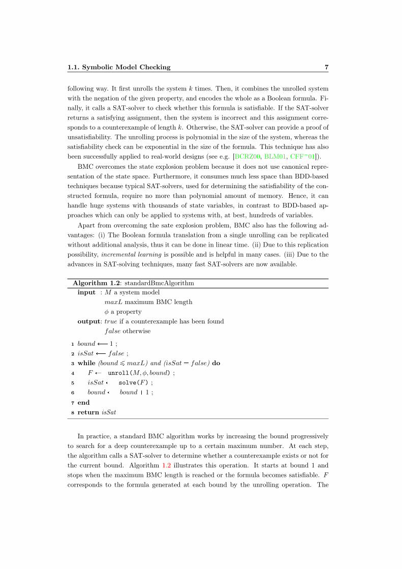
Algorithm 1.2: standardBmcAlgorithminput : M a system model
maxL maximum BMC lengthφ a property
output: true if a counterexample has been foundfalse otherwise
boundÐÝ 1 ;1
isSatÐÝ false ;2
while (bound ¤ maxL) and (isSat false) do3
F ÐÝ unroll(M,φ, bound) ;4
isSatÐÝ solve(F) ;5
boundÐÝ bound 1 ;6
end7
return isSat8
In practice, a standard BMC algorithm works by increasing the bound progressivelyto search for a deep counterexample up to a certain maximum number. At each step,the algorithm calls a SAT-solver to determine whether a counterexample exists or not forthe current bound. Algorithm 1.2 illustrates this operation. It starts at bound 1 andstops when the maximum BMC length is reached or the formula becomes satisfiable. Fcorresponds to the formula generated at each bound by the unrolling operation. The

8 Introduction
function solve() calls the SAT-solver to determine whether F is satisfiable.The speed of the SAT-solver is crucial during the execution because it affects the
performance of the whole BMC operation. When the bound is increased, the number ofvariables in the formula increases linearly, whereas the solving complexity increases expo-nentially. For example, when moving from a bound k to k1, with k k1, the complexityincreases 2n.k to 2n.k
1
, where n is the number of gates in the circuit. This situation impliesthat the deeper the exploration goes, the slower the execution.
During a BMC session, if the maximum number is reached without finding any coun-terexample, no conclusion can be drawn concerning the correctness of the system since thecounterexample may exists at a bound beyond the maximum number. This inability todraw conclusion makes BMC somewhat incomplete compared to BDD-based approaches.Nevertheless, many techniques have been proposed so far to work around this complete-ness issue. We will review some of them in Chapter 3.
The standard BMC method mentioned above is well suited for synchronous systems,a kind of system in which the execution is coordinated by a clock and all variables changetogether at the same time. But if we apply it to asynchronous concurrent systems, a kindof system composed of many components that can communicate and work concurrently,it will fare badly. Due to the inherent interleaved nature of these systems, the number oftimes we have to invoke a SAT-solver will be much larger—maybe an order of magnitude.In addition, some of them tend to produce large formulas sooner. Therefore, the above-mentioned execution slowdown may appear at an early stage because not only the SAT-solver will be invoked many times, but it may also handle large formulas. Hence, thesesystems need more elaborate methods for handling them.
1.2 Synchronous Versus Asynchronous Systems
In this section we will discuss the main differences between synchronous and asynchronoussystems. We will start with the synchronous ones.
1.2.1 Synchronous systems
The synchronous methodology has been used successfully for the design and implemen-tation of safety-critical embedded systems such as flight control systems in flight-by-wireavionics and antiskidding or anticollision equipment on automobiles. They are also presentin other applications such as trains, nuclear plants, and cell phones.
Basically, a synchronous circuit contains the following components:
- circuit inputs,
- gates,
- latches.

1.2. Synchronous Versus Asynchronous Systems 9
The operation in such a circuit is controlled by a global clock. All values in its storagecomponents change simultaneously following the clock signals. During a clock cycle, eachcircuit input receives a random value true or false. The output of a gate is formed by aBoolean combination of its inputs. A latch corresponds to a memory unit with one inputand one output. The inputs of gates and latches are connected to the inputs and outputsof other gates and latches. Consequently, the output of a latch in a given clock-cycle isa Boolean combination of inputs and outputs of latches in the previous clock-cycle. Thebehavior of the whole circuit is entirely predictable because each input reaches its finalvalue before the next clock occurs. In practice, some delay may be needed for each logicaloperation in order to limit the speed at which the system can run. To determine themaximum safe speed, static timing analysis is often used.
Advantages of Synchronous Systems
Here are some of the most important advantages of synchronous systems.
Easier to model Synchronous systems are often modeled with finite state machine(FSM). To model concurrency correctly, it is sometimes necessary to use a combinationof several FSMs for one system. Since synchronous models are deterministic, it is muchmore easier to formally reason about the models and check certain properties, especiallyin case of safety-critical systems.
Easier to design A synchronous circuit can be designed easily in an improvised fashion.For instance, a designer can simply define the combinational logic to compute a givenfunction, and surround it with latches. In addition, nearly all of the most importantdesign-related operations for synchronous systems exist in many of today’s computer-aided design (CAD) tools.
Drawbacks of Synchronous systems
In the synchronous paradigm, time is defined as a sequence of instants between whichnothing interesting happens. In each instant, some events (inputs) occur in the environ-ment, and a reaction (output) is computed instantly by the modeled design. Therefore,despite of all the advantages we discussed above, reasoning and verification based onsynchronous models are meaningful only if a completely synchronous implementation ofthe whole system is possible, and if we are sure that for the implemented system thereaction time (including internal communications) is negligible compared to the rate ofexternal events. Furthermore, it is practically impossible to model a large system usingsynchronous models.

10 Introduction
1.2.2 Asynchronous systems
Asynchronous systems can be found in many applications, ranging from CD players toavionics systems. Their features meet the necessary requirements for assembling large-scale heterogeneous and scalable systems. Typically, they are constructed by combiningseveral hardware components together to form a correct working system. Communicationbetween these components is assured through channels, which are used both to synchronizeoperations and to pass data. Like their synchronous counterparts, asynchronous systemsalso use binary signals. However, they do not use a global clock. Instead, their componentswork concurrently using handshaking between them in order to perform the necessarysynchronization, communication, and sequencing of operations. This mechanism resultsin a behavior similar to local clocks that are not in phase.
Advantages of Asynchronous Systems
Asynchronous systems have numerous advantages. We will describe some of the them.
Low power dissipation Basically, the clock in a synchronous circuit has to control allparts of the circuit including those that are not used in the current computation. Forinstance, even though a floating point unit on a processor may not be used in an ongoinginstruction stream, the clock still has to control the unit. By contrast, for asynchronouscircuits, the components are activated only when needed, so they make signal transitionsonly when performing some work or communicating. Because of this feature, they workfast, yet have low power dissipation.
No clock skew Clock skew refers to the difference in arrival times of the clock signalat different parts of the circuit. The absence of a global clock in synchronous circuitsprevent them from having clock skew problems.
Less electromagnetic interference Electromagnetic interference (EMI) is a kind ofinterference caused by the high speed clock switching all over a chip at approximately thesame time. Asynchronous systems generate less emission of EMI because they use localhandshaking whose signals are not correlated in time.
Easing of global timing issue In systems such as synchronous microprocessors, mostportions of the circuit must be carefully optimized in order to obtain the highest clock rateand to achieve better performance. On the other hand, for asynchronous systems, rarelyused portions of the circuit can be left unoptimized without affecting system performance.
Easier technology migration Basically, integrated circuits are built using differenttechnologies during their lifetime. For instance, early systems may be built with gate ar-rays, while later production may migrate to custom ICs. For asynchronous systems, thereis no need to migrate all system components in order to achieve a greater performance.
1.3. Scope of This Work 11
Migrating only the most critical parts is sufficient. In addition, components with differentdelays can be substituted without altering other elements.
Automatic adaptation to physical properties The delay in a circuit can be affectedby many factors including variations in fabrication, temperature, and power-supply volt-age. Asynchronous systems can adapt themselves to these different factors, and will runas fast as the current physical properties allow.
Drawbacks of Asynchronous Systems
Asynchronous systems have their drawbacks, nonetheless. First of all, due to their com-plexity, they are more difficult to design. Next, the ordering of operations is too difficultto handle, especially for complex systems. Finally, there are not too many CAD tools de-voted to asynchronous circuits. Many of the most essential operations existing in today’sCAD tools such as placement, routing, partitioning, logic synthesis are either need specialmodifications for asynchronous systems, or are not applicable at all.
1.3 Scope of This Work
The main purpose of this work is to build efficient verification techniques for asynchronousconcurrent systems. Because of the pivotal roles these systems assume in a given appli-cation, designers of such systems must keep development and maintenance costs undercontrol and meet nonfunctional constraints on the design of the system, such as cost,power, weight, or the system architecture by itself. But most importantly, they mustassure their customers as well as the certification authorities that both the design and itsimplementation are correct. Otherwise, they may end up shipping unsafe systems to themarket, and the consequences of this action would be catastrophic. To achieve this goal,designers need efficient methods and tools to assist them in verifying the correctness ofthe design. These methods should be built on solid mathematical foundations in order tobe able to reason formally about the operation of the system.
We focus our study on BMC. We aim at developing BMC methods supported bytools for analyzing the behavior of asynchronous concurrent systems and verify theircorrectness, considering all the benefits and challenges in this area. BMC is traditionallyused for verifying synchronous systems because the characteristics of these systems matchwell a BMC operation. However, in this work, we apply it to asynchronous systems. Thefollowing points explain our choice.
- There exist already numerous BDD-based methods and tools for asynchronous con-current systems. Most of them have been successfully applied in the industry. Still,the state explosion problem limits the size of the problem they can solve. On theother hand, SAT-based methods do not have this kind of problem, thus can handlemuch bigger systems.
12 Introduction
- With the success story of BMC with synchronous systems, we believe that with alittle effort, it is also possible to repeat this success for asynchronous systems. Forthis reason, we are interesting in building verification methods and tools, based onBMC, for asynchronous systems.
- SAT-solving methods and tools continue to improve. Not only they become faster,but the size of the formulas they can handle continues to grow. Therefore, webelieve that even though asynchronous systems are complex, using these state-of-the-art solvers will help to tackle the problems.
To handle asynchronous concurrent systems properly, and to tackle all the BMC prob-lems explained in the previous section, two main related tasks should be considered. First,developing encoding techniques that provide compact Boolean formulas to be solved by aSAT-solver. Second, building efficient unrolling techniques to minimize the bound neededfor finding a counterexample.
We propose in this thesis several encoding techniques for systems modeled as transitionsystems: methods for checking reachability properties as well as for checking propertiesexpressed in linear temporal logic (LTL). We also propose methods for minimizing thebound during the BMC operation. We have implemented all these methods in a BMCtoolset for asynchronous systems.
1.4 Structure of the Thesis
The rest of this thesis is structured as follows. In Chapter 2 we give all the definitionswe need throughout the report. In Chapter 3 we review most of the important BMCtechniques that exist in the literature. We introduce our approaches in Chapters 4 and 6.In Chapter 7, we describe our BMC toolset. Case studies with experimentation resultsare shown in Chapter 8. We conclude the thesis in Chapter 9 and give some possiblefuture directions.
Chapter 2
Background
In this chapter, we present the definitions and notations to be used throughout the report.We will first describe the transition system model, along with other popular formalismsfor modeling concurrent systems. Next, we will explain what a property is and how toexpress it formally. After that, we will discuss the satisfiability problem, and review someof the most effective methods for solving it. Finally, we will show, with an example, howto use BMC to verify safety properties.
2.1 Transition Systems
In order to verify the correctness of a system, it is necessary to use an appropriate formal-ism that can describe clearly the system’s behavior. Furthermore, the model should beable to capture the properties of interest. For finite concurrent systems, the behavior ismainly determined by three elements: states, transitions, and computations. A state cor-responds to a group of variables needed for describing the system at a particular instant.When an action or event occurs, the system changes from one state to another, and thevalues of the state before and after such an event determine a transition. A computationor also execution path is formed by an infinite sequence of states, in which two consecutivestates are connected via a transition. In this section, we discuss a well-known model calledtransition system (TS) [Arn94], which is also the one we use in our study.
2.1.1 DefinitionsDefinition 2.1.1 (Transition system)A transition system is tuple A pS,Σ, T, s0q where
- S is a non-empty set of states;
- Σ is a non-empty set of events;
- T S Σ S is a transition relation whose elements are called transitions;
14 Background
s0
s1 s2
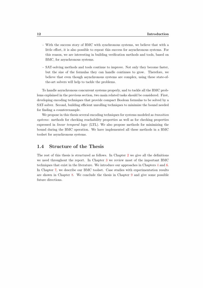
s3 s4 s5 s6
(A)
a
d bd
d
c
Figure 2.1: A Transition system.
- s0 is the initial state.
A transition from a state s to a state s1 is written s eÝÑ s1 or ps, e, s1q where e denotes
the event associated to the transition.
A transition system can be represented as a directed graph whose nodes correspondto the states, and the edges to the transitions. The transitions are labeled with theirassociated events.
Example 2.1.1 Figure 2.1 depicts an example of TS. We have A pS,Σ, T, soq whereS ts0, s1, s2, s3, s4, s5, s6u; Σ ta, b, c, du; T ts0
aÝÑ s1, s0
dÝÑ s2, s1
dÝÑ s3, s1
dÝÑ
s4, s2bÝÑ s5, s2
cÝÑ s6u.
Definition 2.1.2 (Enabling)Let A pS,Σ, T, s0q be a transition system, and e an event in Σ. e is enabled at states if D s e
ÝÑ s1 P T . If e is enabled, it can fire. The set of enabled events at state s isdenoted by Epsq.
Definition 2.1.3 (Run)Let A pS,Σ, T, s0q be a transition system. A run or execution from a state s is asequence of transitions
σ s0e0ÝÑ s1
e1ÝÑ . . .ek1ÝÑ sk (2.1)
such that s0 s and @i ¥ 0, sieiÝÑ si1 P T . A state sk is reachable if there exists a
run from the initial state s0 to sk.
It is, therefore, possible to construct a run from a set of states S0 to a set of states Skdenoted as S0
E0ÝÑ S1E1ÝÑ . . .
Ek1ÝÑ Sk, where Ei designs the set of events that fire from
Si.
Definition 2.1.4 (To Set)Given a transition system A pS,Σ, T, s0q. Let s P S be a state. We define the set Topsqas follows:

2.1. Transition Systems 15
FrompSi1q
s1 s2 s3 s4 s5 s6
TopSiq
s7 s8 s9 s10
Si
Si1
Figure 2.2: To and From sets.
Topsq ts1 P S | De P Σ, seÝÑ s1 P T u (2.2)
Likewise, given a set of states P S the set TopP q is a set P 1 S such that@s1 P P 1, Ds P P such that s1 P Topsq.
Definition 2.1.5 (From Set)Given a transition system A pS,Σ, T, s0q. Let s1 P S be a state. We define the setFromps1q as follows:
Fromps1q ts P S | De P Σ, seÝÑ s1 P T u (2.3)
Likewise, given a set of states P 1 S the set FrompP 1q is a set P S such that@s1 P P 1, Ds P P, s P Fromps1q.
Note that in a given run S0E0ÝÑ S1
E1ÝÑ . . .Ek1ÝÑ Sk, we always have TopSiq Si1,
but sometimes we may have FrompSi1q Si. This situation happens when some of thestates in Si has no outgoing transitions (see Figure 2.2).
2.1.2 Symbolic Representation
To represent transition systems symbolically, we use Boolean algebras [Kop89]. The rep-resentation is needed when we construct the Boolean formulas during the BMC unrollingoperation. We will start this section by describing Boolean algebras, then show how touse them for representing a transition system.
Definition 2.1.6 (Boolean Algebra)A Boolean algebra is a tuple pB,, ., 0, 1q, where B is a set; an . are binary operators onB satisfying the commutative and distributive law; 0 and 1 are elements of B representingthe neutral element for and . respectively. i.e., @ b P B, b 0 b and b . 1 b.
Each element b P B has a complement b P B such that b b 1 and b . b 0.
16 Background
Definition 2.1.7 (Boolean Function)A Boolean function is an n-variable logic function f : Bn Ñ B, where B t0, 1u, and ftransforms each element pv0, . . . , vn1q P B
n into an element of B.A Boolean function f is a zero function if fpv0, . . . , vn1q 0, @pv0, . . . , vn1q P B
n.Likewise, a Boolean function f is a one function if fpv0, . . . , vn1q 1, @pv0, . . . , vn1q P
Bn.Each element of Bn is called vertex. A literal is either a variable vi or its complement
vi. A cube c is a set of literals, such that if vi P c then vi R c and vice versa.
Example 2.1.2 Below are some interesting examples of Boolean algebras.
- pB,_,^, 0, 1q, where B t0, 1u; _ and ^ correspond to the logical operators ORand AND respectively.
- pFnpBq,, ., 0, 1q, where FnpBq is the set of n-variable logic functions on B; and .represent the addition and multiplication of n-variable logic functions respectively;0 and 1 correspond to the zero and one functions respectively.
- p2S ,Y,X,H, Sq, where S is a set; Y and X correspond to the set operators unionand intersection respectively.
We will now give a symbolic representation of a transition system using Boolean alge-bra. Given a TS A pS,Σ, T, s0q. We can then build a Boolean algebra p2S ,Y,X,H, Sqfrom the set of states S. However, since in BMC, we are dealing with Boolean variablesrather than sets, we need to find a way to map each state in S into Boolean variables. Inthis way, we will have an encoding that reasons in terms of logic operators such as _ and^, rather than set operators such as Y and X.
The mapping can be done as follows. We represent each state s P S by en encodingfunction Q : S Ñ Bn such that n ¥ rlog2p|S|qs and B t0, 1u. That is, given aset of Boolean variables V tv0, . . . , vn1u each state s P S is encoded into a vertexpv0, . . . , vn1q P B
n. We choose n |S|, and for each state, all variables in its associatedvertex equal zero except for the one which has the same index as the state. i.e. given astate si, we have:
si Ø pv0 0, . . . , vi 1, . . . , vn1 0q (2.4)
Example 2.1.3 Assume |S| 4. Then, we have n 4, i.e V tv0, v1, v2, v3u,and each state is mapped as follows s0 Ø p1, 0, 0, 0q, s1 Ø p0, 1, 0, 0q, s2 Ø p0, 0, 1, 0q,s3 Ø p0, 0, 0, 1q.
Any set of states P S can be represented by a characteristic (Boolean) functionXP : Bn Ñ B that evaluates to 1 for those vertices in Bn that correspond to states in P ,encoded using Q.

2.2. Other Models for Concurrent Systems 17
Using the state encoding above, the characteristic function of a set of states P can beexpressed by the product of those variables that evaluate to 1 for each state in P .
Formally, we have:
XP ©siPP
vi (2.5)
This kind of characteristic function is much common in Petri net-based methods suchas the one in [OTK04], but in this work, we apply it to transition systems.
Example 2.1.4 As a an example, consider the TS A depicted in Figure 2.1. We have:
Xts0,s1,s2u v0 ^ v1 ^ v2; Xts3u v3;
It is also possible to represent each state using the binary number equivalent to thestate’s index. This representation requires at least log2p|S|q Boolean variables. For in-stance, assume |S| 8, then we need n log2p8q 3 variables to represent each state,i.e. V tv0, v1, v2u. In binary number with three variables, we have 0 000, 1 001,2 010, 3 011, etc. Thus, each state is mapped as follows s0 Ø p0, 0, 0q, s1 Ø p0, 0, 1q,s2 Ø p0, 1, 0q, s3 Ø p0, 1, 1q, etc. For each state, the number of variables that have thevalue 1 varies from 0 to n. Therefore, the characteristic function XP given in equation(2.5) does not apply for this representation. Rather, it is defined as follows. Assumewe have a set of states P ts0, s1, s2u, and n 3. Then the function XP is given asXP pv0^ v1^ v2q _ pv0^ v1^ v2q _ pv0^ v1^ v2q. As we can see, the derived Booleanformula is larger than the one in Example 2.1.4. Hence, this representation is not quiteappropriate for SAT-based approaches because it will give extra work to the solving pro-cess. It is much more common in BDD-based methods (see e.g. [Pen03]). Figure 2.3depicts the difference between these two representations.
2.2 Other Models for Concurrent Systems
In this section, we discuss other important formalisms for modeling concurrent systems.Namely, Kripke structure, Petri nets, and automata.
2.2.1 Kripke Structure
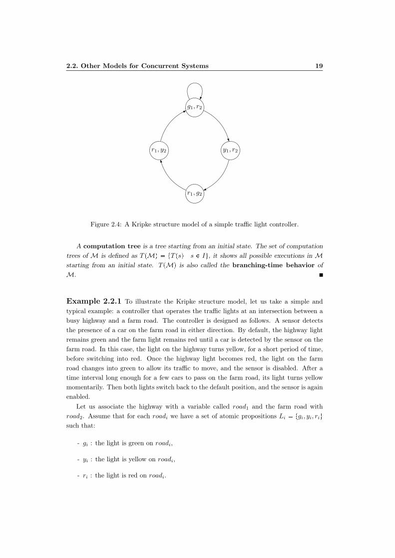
A Kripke structure [CGP99] is a formalism used for describing the behavior of reactivesystems, i.e. systems that interact frequently with their environment. It is a graph-based model, whose nodes represent the system’s states and whose edges represent thetransitions between states. This formalism also uses a labeling function that maps eachnode with a set of properties that are true in the corresponding state (See Figure 2.4).Below is a formal definition of a Kripke structure.
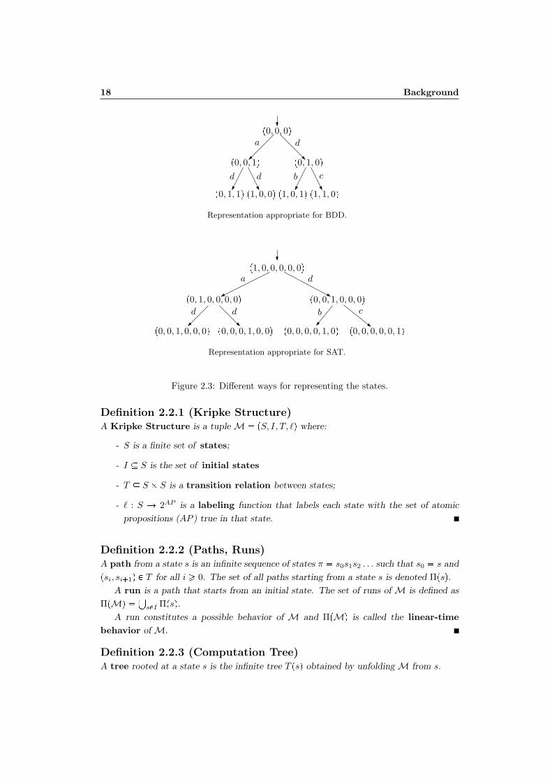
18 Background
p0, 0, 0q
p0, 0, 1q p0, 1, 0q
p0, 1, 1q p1, 0, 0q p1, 0, 1q p1, 1, 0q
Representation appropriate for BDD.
a
d bd
d
c
p1, 0, 0, 0, 0, 0q
p0, 1, 0, 0, 0, 0q p0, 0, 1, 0, 0, 0q
p0, 0, 1, 0, 0, 0q p0, 0, 0, 1, 0, 0q p0, 0, 0, 0, 1, 0q p0, 0, 0, 0, 0, 1q
Representation appropriate for SAT.
a
d bd
d
c
Figure 2.3: Different ways for representing the states.
Definition 2.2.1 (Kripke Structure)A Kripke Structure is a tuple M pS, I, T, `q where:
- S is a finite set of states;
- I S is the set of initial states
- T S S is a transition relation between states;
- ` : S Ñ 2AP is a labeling function that labels each state with the set of atomicpropositions (AP ) true in that state.
Definition 2.2.2 (Paths, Runs)A path from a state s is an infinite sequence of states π s0s1s2 . . . such that s0 s andpsi, si1q P T for all i ¥ 0. The set of all paths starting from a state s is denoted Πpsq.
A run is a path that starts from an initial state. The set of runs of M is defined asΠpMq
sPI Πpsq.
A run constitutes a possible behavior of M and ΠpMq is called the linear-timebehavior of M.
Definition 2.2.3 (Computation Tree)A tree rooted at a state s is the infinite tree T psq obtained by unfolding M from s.
2.2. Other Models for Concurrent Systems 19
r1, y2
g1, r2
y1, r2
r1, g2
Figure 2.4: A Kripke structure model of a simple traffic light controller.
A computation tree is a tree starting from an initial state. The set of computationtrees of M is defined as T pMq tT psq | s P Iu, it shows all possible executions in Mstarting from an initial state. T pMq is also called the branching-time behavior ofM.
Example 2.2.1 To illustrate the Kripke structure model, let us take a simple andtypical example: a controller that operates the traffic lights at an intersection between abusy highway and a farm road. The controller is designed as follows. A sensor detectsthe presence of a car on the farm road in either direction. By default, the highway lightremains green and the farm light remains red until a car is detected by the sensor on thefarm road. In this case, the light on the highway turns yellow, for a short period of time,before switching into red. Once the highway light becomes red, the light on the farmroad changes into green to allow its traffic to move, and the sensor is disabled. After atime interval long enough for a few cars to pass on the farm road, its light turns yellowmomentarily. Then both lights switch back to the default position, and the sensor is againenabled.
Let us associate the highway with a variable called road1 and the farm road withroad2. Assume that for each roadi we have a set of atomic propositions Li tgi, yi, riusuch that:
- gi : the light is green on roadi,
- yi : the light is yellow on roadi,
- ri : the light is red on roadi.
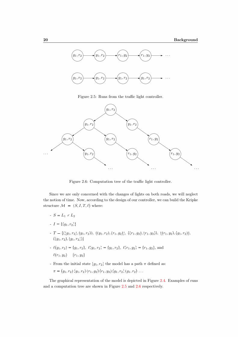
20 Background
g1, r2 y1, r2 r1, g2 r1, y2 . . .
g1, r2 g1, r2 g1, r2 g1, r2 . . .
Figure 2.5: Runs from the traffic light controller.
g1, r2
g1, r2
g1, r2
. . .
y1, r2
y1, r2
y1, r2
r1, g2
r1, g2
. . .
r1, y2
. . . . . .
Figure 2.6: Computation tree of the traffic light controller.
Since we are only concerned with the changes of lights on both roads, we will neglectthe notion of time. Now, according to the design of our controller, we can build the Kripkestructure M pS, I, T, `q where:
- S L1 L2
- I tpg1, r2qu
- T tppg1, r2q, py1, r2qq, ppy1, r2q, pr1, g2qq, ppr1, g2q, pr1, y2qq, ppr1, y2q, pg1, r2qq,
ppg1, r2q, pg1, r2qqu
- `pg1, r2q tg1, r2u, `py1, r2q ty1, r2u, `pr1, g2q tr1, g2u, and
`pr1, y2q tr1, y2u
- From the initial state pg1, r2q the model has a path π defined as:
π pg1, r2q py1, r2q pr1, g2q pr1, y2q pg1, r2q pg1, r2q . . .
The graphical representation of the model is depicted in Figure 2.4. Examples of runsand a computation tree are shown in Figure 2.5 and 2.6 respectively.
2.2. Other Models for Concurrent Systems 21
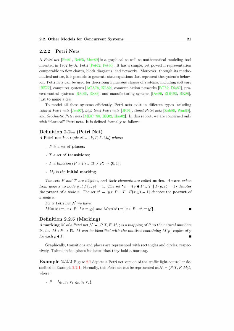
2.2.2 Petri Nets
A Petri net [Pet81, Rei85, Mur89] is a graphical as well as mathematical modeling toolinvented in 1962 by A. Petri [Pet62, Pet66]. It has a simple, yet powerful representationcomparable to flow charts, block diagrams, and networks. Moreover, through its mathe-matical nature, it is possible to generate state equations that represent the system’s behav-ior. Petri nets can be used for describing numerous classes of systems, including software[BE77], computer systems [ACA78, KL82], communication networks [BT82, Dia87], pro-cess control systems [BM86, DS83], and manufacturing systems [Des89, ZDR92, BK86],just to name a few.
To model all these systems efficiently, Petri nets exist in different types includingcolored Petri nets [Jen97], high level Petri nets [JR91], timed Petri nets [Zub80, Wan98],and Stochastic Petri nets [MBC98, BK02, Haa02]. In this report, we are concerned onlywith “classical” Petri nets. It is defined formally as follows.
Definition 2.2.4 (Petri Net)A Petri net is a tuple N pP, T, F,M0q where:
- P is a set of places;
- T a set of transitions;
- F a function pP T q Y pT P q Ñ t0, 1u;
- M0 is the initial marking.
The sets P and T are disjoint, and their elements are called nodes. An arc existsfrom node x to node y if F px, yq 1. The set x ty P P Y T | F py, xq 1u denotesthe preset of a node x. The set x ty P P Y T | F px, yq 1u denotes the postset ofa node x.
For a Petri net N we have:MinpN q tx P P | x Hu and MaxpN q tx P P | x Hu.
Definition 2.2.5 (Marking)A marking M of a Petri net N pP, T, F,M0q is a mapping of P to the natural numbersN, i.e. M : P Ñ N. M can be identified with the multiset containing Mppq copies of pfor each p P P .
Graphically, transitions and places are represented with rectangles and circles, respec-tively. Tokens inside places indicates that they hold a marking.
Example 2.2.2 Figure 2.7 depicts a Petri net version of the traffic light controller de-scribed in Example 2.2.1. Formally, this Petri net can be represented asN pP, T, F,M0q,where:
- P tg1, y1, r1, g2, y2, r2u,
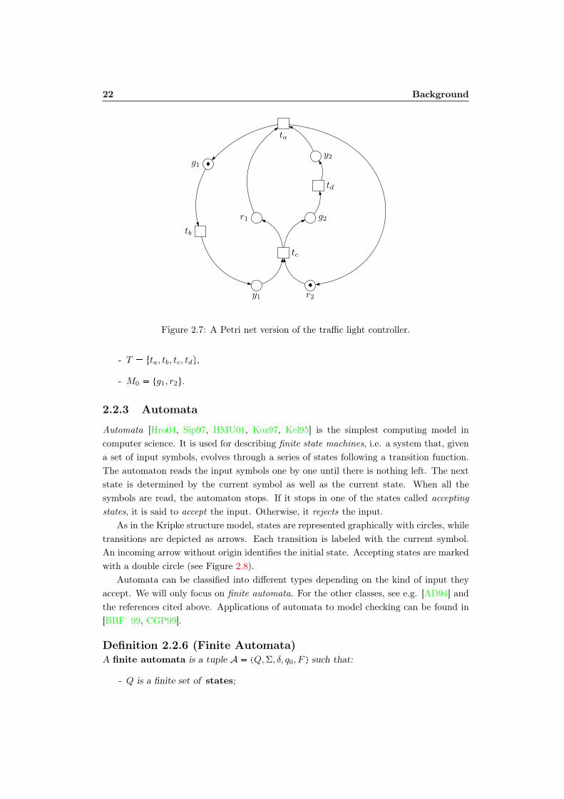
22 Background
g1
y1
r2
r1
y2
g2
tb
tc
ta
td
Figure 2.7: A Petri net version of the traffic light controller.
- T tta, tb, tc, tdu,
- M0 tg1, r2u.
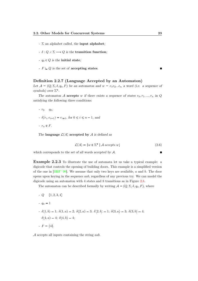
2.2.3 Automata
Automata [Hro04, Sip97, HMU01, Koz97, Kel95] is the simplest computing model incomputer science. It is used for describing finite state machines, i.e. a system that, givena set of input symbols, evolves through a series of states following a transition function.The automaton reads the input symbols one by one until there is nothing left. The nextstate is determined by the current symbol as well as the current state. When all thesymbols are read, the automaton stops. If it stops in one of the states called acceptingstates, it is said to accept the input. Otherwise, it rejects the input.
As in the Kripke structure model, states are represented graphically with circles, whiletransitions are depicted as arrows. Each transition is labeled with the current symbol.An incoming arrow without origin identifies the initial state. Accepting states are markedwith a double circle (see Figure 2.8).
Automata can be classified into different types depending on the kind of input theyaccept. We will only focus on finite automata. For the other classes, see e.g. [AD94] andthe references cited above. Applications of automata to model checking can be found in[BBF99, CGP99].
Definition 2.2.6 (Finite Automata)A finite automata is a tuple A pQ,Σ, δ, q0, F q such that:
- Q is a finite set of states;
2.2. Other Models for Concurrent Systems 23
- Σ an alphabet called, the input alphabet;
- δ : Q Σ ÝÑ Q is the transition function;
- q0 P Q is the initial state;
- F Q is the set of accepting states.
Definition 2.2.7 (Language Accepted by an Automaton)Let A pQ,Σ, δ, q0, F q be an automaton and w e1e2...en a word (i.e. a sequence ofsymbols) over Σ.
The automaton A accepts w if there exists a sequence of states r0, r1, ..., rn in Q
satisfying the following three conditions:
- r0 q0,
- δpri, ei1q ri1, for 0 ¤ i ¤ n 1, and
- rn P F .
The language LpAq accepted by A is defined as
LpAq tw P Σ | A accepts wu (2.6)
which corresponds to the set of all words accepted by A.
Example 2.2.3 To illustrate the use of automata let us take a typical example: adigicode that controls the opening of building doors. This example is a simplified versionof the one in [BBF99]. We assume that only two keys are available, a and b. The dooropens upon keying in the sequence aab, regardless of any previous try. We can model thedigicode using an automaton with 4 states and 8 transitions as in Figure 2.8.
The automaton can be described formally by writing A pQ,Σ, δ, q0, F q, where
- Q t1, 2, 3, 4u
- q0 1
- δp1, bq 1; δp1, aq 2; δp2, aq 3; δp2, bq 1; δp3, aq 3; δp3, bq 4;
δp4, aq 4; δp4, bq 4;
- F t4u.
A accepts all inputs containing the string aab.

24 Background
1 2 3 4
a
b
a b
b a a, b
Figure 2.8: An automaton model of a digicode.
2.3 Linear Temporal Logic
Temporal logic [Eme90, CW96] is a form of logic used for describing the behavior of con-current systems. It is aimed at expressing succession of events without mentioning timeexplicitly. It uses simple and clear notations, called temporal operators, that correspondroughly to words in a natural language such as until, next, and eventually. To expressproperties of states, the logic also uses atomic propositions combined with Boolean con-nectives such as , ^, and _.
In this section, we will focus on a temporal logic called linear temporal logic (LTL)[GPSS80, Lam80, BBF99] which uses the following temporal operators:
- X (“next”) indicates that the next state satisfies a property;
- F (“in the future or eventually”) specifies that a future state on the path will satisfya property;
- G (“globally or always”) implies that a property will hold at all the future states inthe path;
- U (“until”) relates two properties. It states that a property holds along the pathuntil a second property is verified.
- R (“release”) is the logical dual of U. It requires that the second property holds alongthe path up to the first state where the first property holds (or forever if such a statedoes not exist).
Let P be a set of atomic propositions. The syntax and semantics of an LTL formulais given by the following definitions.
Definition 2.3.1 (Syntax)The set of LTL formulas on the set P is defined by the grammar ψ p | ψ |ψ1 ^
ψ2 |ψ1 _ ψ2 |Xψ |ψ1 U ψ2 , where p ranges over P .
Definition 2.3.2 (semantics)Let ξ u0u1u2 . . . be an infinite word over the alphabet 2P . Let ψ be an LTL formula.In the semantics below, ξ ( ψ means ξ models ψ. We also define ξpiq ui and ξi
uiui1 . . . for i P N. The semantics of LTL is then given as follows:
2.3. Linear Temporal Logic 25
- ξ ( p iff p P ξp0q, for p P P
- ξ ( ψ1 ^ ψ2 iff ξ ( ψ1 and ξ ( ψ2,
- ξ ( ψ1 _ ψ2 iff ξ ( ψ1 or ξ ( ψ2,
- ξ ( X ψ iff ξ1 ( ψ,
- ξ ( ψ1 U ψ2 if Di rξi ( ψ2 and @j, j i we have ξj ( ψ1s,
We will also use the abbreviations true p _ p and false true. The temporaloperators F, G, and R are derived from the above definition as follows:
Fψ trueUψ (2.7)
Gψ falseRψ (2.8)
ψ1 R ψ2 p ψ1 U ψ2q (2.9)
Example 2.3.1 Let us give some examples of LTL formula:
- GpbarOpenUmidnightq reads “it is always true that the bar opens until midnight,”
- XpourTrainq reads “our train will come just next,”
- G pcritSec1^ critSec2q reads “both processes will never be in their critical sectionat the same time,”
- GpReq Ñ FSatq reads “any request will eventually be satisfied.”
For concurrent systems, the next-time operator X does not have significant meaningbecause, in these types of systems, it is not really important to make a distinction betweenone execution step and two or more subsequent steps. These steps are considered to beobservationally equivalent, especially for high level abstract specifications. For that rea-son, some researchers do not include this operator when they study LTL with concurrentsystems (e.g. [Sor02]). The resulted logic is often known as LTL-X. In [Lam83], Lamportgives a detailed explanation as to why the next-time operator can be omitted in temporallogic.
Some people also focus their study on the logic known as PLTL which is a type ofLTL combined with past operators such as Y (yesterday), O (once), and H (historically)[BC03, BHJ06]. In theoretical point of view, there is no big difference between PLTLand future-only LTL since they both have the same degree of expressiveness. In practice,however, past operators can be more useful as they keep specifications short and simple.Hence, they can help model checker users to formulate the desired properties in a moresuccinct and natural way.
26 Background
Negative Normal Form
Many LTL-based model checking methods require the formula to be written into negativenormal form (NNF)—i.e. a formula in which every negation appears only before a literal—using the operators _,^ X, U, and R. NNF formulas can be obtained by applying thefollowing equivalences:
true p_ p (2.10)
false true (2.11)
ψ1 ^ ψ2 p ψ1 _ ψ2q (2.12)
ψ1 R ψ2 p ψ1 U ψ2q (2.13)
F ψ true U ψ (2.14)
Gψ F ψ (2.15)
Logic for Nondeterministic Choices
The logic LTL can only describe events along a single computation path. Therefore, itcannot express the possibility of nondeterministic choices that may exist along an execu-tion (run) at some instants. Because of this feature, LTL formulas are also called pathformulas. To express nondeterministic choices, one can use the logic known as compu-tation tree logic (CTL) [EH86, CES86] whose formulas may contain the following pathquantifiers:
- A, known as universal path quantifier, suggests that a property is satisfied by all thecomputation paths starting from the current state;
- E, known as existential path quantifier, illustrates that there exists a computationpath from the current state that satisfies a property.
Example 2.3.2 To see the difference between CTL and LTL representations, let ustake again one of the formulas from Example 2.3.1. In LTL, the statement “both processeswill never be in their critical section at the same time,” is expressed as AG pcritSec1 ^critSec2q
More examples of properties expressed in temporal logic can be found in [BBF99,Pnu77]. The complexity of temporal logic with model checking is discussed in [Shn02,Sa85].
2.4 Satisfiability Problem
The Boolean satisfiability problem (SAT) is a decision problem of finding if there existssome assignment of the values 0 and 1 to the variables in a Boolean formula that makesit evaluate to 1 (true). If this assignment exists, the formula is said to be satisfiable.
2.4. Satisfiability Problem 27
The formula to be solved is often written in conjunctive normal form (CNF), that isa conjunction of clauses with disjunctive literals as in the following example.
Example 2.4.1 The CNF formula px1_ x2_x3q^ px1_x3q^ p x2_ x3q has thesatisfying assignment x1 1, x2 1, x3 0.
SAT has been applied to many fields in computer science including problems in elec-tronic design automation (EDA) [FDK98, CG96, DKMW93, SSA91], microprocessor ver-ification [VB01], field-programmable gate array (FPGA) layout [NASR04], automatic testpattern generation (ATPG) [SBSV96, TGH97], to name but a few. (See [GPFW97] for acomplete list of applications that can be formulated as SAT.)
Although, SAT belongs to the class of NP-complete problems [Coo71], numerous stud-ies have been conducted to find better algorithms and methods for it. Some of them aresoftware-related approaches [GPD97], while others consist in customizing the hardwareitself to match the requirements of SAT [AS97, SYSN01, SdBF04]. As a result, manypractical SAT instances can now be solved in minutes, or even seconds on a regular com-puter. But since no one has ever proven that all SAT problems can be solved in polynomialtime, there must be out there some SAT instance which takes huge amount of time tosolve. Note that, interesting SAT benchmarks are available online at [Vel, DIM, SAT].Benchmarks designed especially for BMC can also be found in [Zar05, Zar04].
In practice, there exist two classes of algorithms for solving SAT: incomplete andcomplete algorithms. Based on heuristic search algorithms, incomplete algorithms canprovide results very fast. Still, they cannot prove unsatisfiability and, in some cases,terminate without giving any result at all. For that reason, most state-of-the-art SATsolvers use complete algorithms which can always lead to a result and are able to proveunsatisfiability. We will describe two well-known algorithms for solving SAT. First, acomplete algorithm known as DPLL . Second, an incomplete one invented by Stålmarck.
2.4.1 DPLL Algorithm
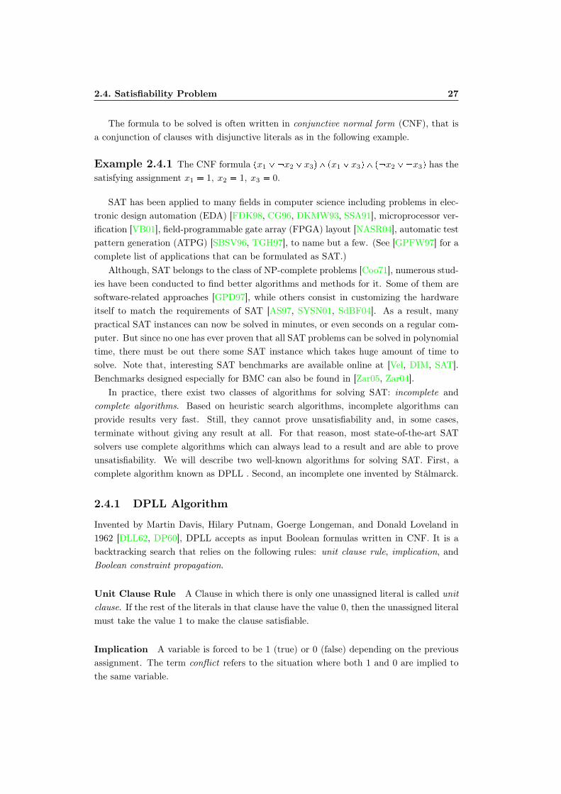
Invented by Martin Davis, Hilary Putnam, Goerge Longeman, and Donald Loveland in1962 [DLL62, DP60], DPLL accepts as input Boolean formulas written in CNF. It is abacktracking search that relies on the following rules: unit clause rule, implication, andBoolean constraint propagation.
Unit Clause Rule A Clause in which there is only one unassigned literal is called unitclause. If the rest of the literals in that clause have the value 0, then the unassigned literalmust take the value 1 to make the clause satisfiable.
Implication A variable is forced to be 1 (true) or 0 (false) depending on the previousassignment. The term conflict refers to the situation where both 1 and 0 are implied tothe same variable.

28 Background
Algorithm 2.1: dpllinput : formula in CNFoutput: sat or unsat
while 1 do1
decide() ;2
while 1 do3
statusÐÝ bcp() ;4
if status conflicts then5
blevelÐÝ analyzeConflict() ;6
if blevel 0 then7
return unsat ;8
else9
backtrack(blevel) ;10
end11
else if status satisfiable then12
return sat ;13
else14
break ;15
end16
end17
end18
Boolean constraint Propagation (BCP) It refers to the task of applying the unitclause rule iteratively until there is no unit clause available.
Algorithm 2.1 depicts a simplified version of DPLL. The function decide() choosesan unassigned variable to branch and gives it a value. bcp() carries out BCP operationuntil a satisfying assignment is found, or until a conflict occurs. When conflict occurs,analyzeConflict() determines the level at which to backtrack. This level correspondsto a variable that has not been assigned both ways (1 and 0). If no such a variable exists,the formula is unsatisfiable. A new clause, known as conflict clause, which describes theconflicting branch can also be added during the conflict analysis in order to avoid searchingthe same path again in the future. backtrack (blevel) flips the branching variable atblevel, and undoes all implications up to that level.
DPLL is implemented in many solvers such as ZChaff [MMZ01], Berkmin [GN02],Sato [Zha97], and Grasp [SS99] to name but a few.
2.4.2 Stålmarck’s Algorithm
Stålmarck’s k-saturation algorithm [SS00] is based on the so-called dilemma proof system,which is used for proving whether a propositional logic formula is a tautology. Here, k
2.4. Satisfiability Problem 29
represents a natural number called saturation level. The algorithm exhaustively searchesfor a proof of depth k for a given formula. It runs fast with a time complexity Opn2k1q,where n corresponds to the size of the formula. This method is known to be useful forverifying properties of industrial designs, in which, k ¤ 2 appears to be enough in mostcases. Unlike DPLL, Stalmårck’s algorithm can take non-CNF formulas as input. Inaddition, implication (ñ), and equivalence (ô) are also allowed. Before describing thealgorithm, we will first review some terminologies used in the dilemma proof system.
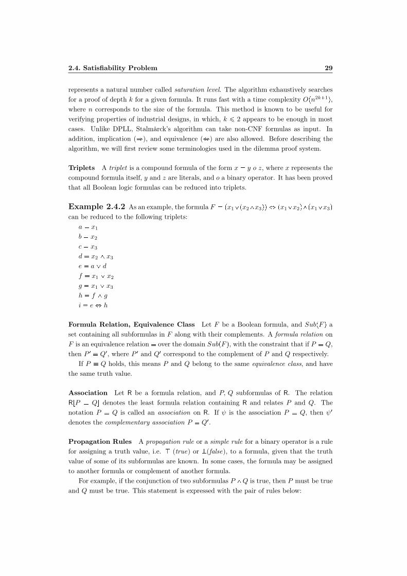
Triplets A triplet is a compound formula of the form x y o z, where x represents thecompound formula itself, y and z are literals, and o a binary operator. It has been provedthat all Boolean logic formulas can be reduced into triplets.
Example 2.4.2 As an example, the formula F px1_px2^x3qq ô px1_x2q^px1_x3q
can be reduced to the following triplets:a x1
b x2
c x3
d x2 ^ x3
e a_ d
f x1 _ x2
g x1 _ x3
h f ^ g
i eô h
Formula Relation, Equivalence Class Let F be a Boolean formula, and SubpF q aset containing all subformulas in F along with their complements. A formula relation onF is an equivalence relation over the domain SubpF q, with the constraint that if P Q,then P 1 Q1, where P 1 and Q1 correspond to the complement of P and Q respectively.
If P Q holds, this means P and Q belong to the same equivalence class, and havethe same truth value.
Association Let R be a formula relation, and P, Q subformulas of R. The relationRrP Qs denotes the least formula relation containing R and relates P and Q. Thenotation P Q is called an association on R. If ψ is the association P Q, then ψ1
denotes the complementary association P Q1.
Propagation Rules A propagation rule or a simple rule for a binary operator is a rulefor assigning a truth value, i.e. J (true) or K(false), to a formula, given that the truthvalue of some of its subformulas are known. In some cases, the formula may be assignedto another formula or complement of another formula.
For example, if the conjunction of two subformulas P ^Q is true, then P must be trueand Q must be true. This statement is expressed with the pair of rules below:

30 Background
P ^Q J
P J
P ^Q J
Q J(2.16)
Other interesting rules for ^ include:
P J
P ^Q Q
Q J
P ^Q P(2.17)
P K
P ^Q K
Q K
P ^Q K(2.18)
P Q
P ^Q P
P Q
P ^Q Q(2.19)
Dilemma Rule The dilemma rule is a branching rule for deriving new equivalencerelation from a formula relation. It has the form below:
R
RrP Qs RrP Qs
π0 π1
R0 R1
R0 XR1
(2.20)
The dilemma rule can be interpreted as follows: first, two subformulas P and Q aretaken from a formula relation R. P and Qmust be from different, but non-complementary,equivalence classes in R. Then, two derivations π1 and π2 are built from the relationsRrP Qs and RrP Qs respectively. This leads to new equivalence classes R0 andR1. Finally, all common associations in R0 and R1 are combined in order to form theintersection R0 XR1.
The Dilemma Proof system
Recall that the dilemma proof system is used for proving whether a given formula is atautology. Briefly put, it works in the following way. At the beginning, the formula isassumed to be false. It is first decomposed into set of triplets. Then, the propagationrules are applied to its subformulas to determine if a contradiction exists. If yes, then theformula is a tautology. Otherwise, the formula is false. The dilemma rule is used only ifnone of the propagation rules can be applied. If still a contradiction is found from theleft and right branch of the dilemma rule, then the formula is a tautology. More detailedexplanation about the dilemma proof system can be found in [SS00].
To implement the dilemma proof system, Stålmarck introduced the k-saturation al-gorithm which has two parts: 0-saturation, used for implementing the propagation rules,and k-saturation (with k ¥ 1), used for the dilemma rule. The formula to be provedis represented as a set of triplets. Starting from a given relation, the algorithm tries toderive a new relation by applying some rules related to the triplets. The given relationcorresponds to the one obtained after assuming that the formula is false. This is often
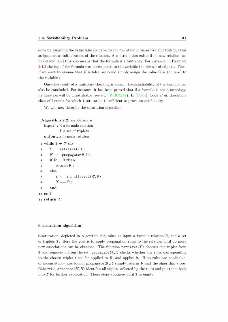
2.4. Satisfiability Problem 31
done by assigning the value false (or zero) to the top of the formula tree and then put thisassignment as initialization of the relation. A contradiction exists if no new relation canbe derived, and this also means that the formula is a tautology. For instance, in Example2.4.2 the top of the formula tree corresponds to the variable i in the set of triplets. Thus,if we want to assume that F is false, we could simply assign the value false (or zero) tothe variable i.
Once the result of a tautology checking is known, the satisfiability of the formula canalso be concluded. For instance, it has been proved that if a formula is not a tautology,its negation will be unsatisfiable (see e.g. [WBCG00]). In [CG05], Cook et al. describe aclass of formula for which 1-saturation is sufficient to prove unsatisfiability.
We will now describe the saturation algorithm.
Algorithm 2.2: zeroSaturateinput : R a formula relation
T a set of tripletsoutput: a formula relation
while T H do1
tÐÝ retrieve(T) ;2
R1 ÐÝ propagate(R,t) ;3
if R1 R then4
return R ;5
else6
T ÐÝ TY affected(R1,R) ;7
R1 ÐÝ R ;8
end9
end10
return R ;11
0-saturation algorithm
0-saturation, depicted in Algorithm 2.2, takes as input a formula relation R, and a setof triplets T . Here the goal is to apply propagation rules to the relation until no morenew associations can be obtained. The function retrieve(T) chooses one triplet fromT and removes it from the set. propagate(R,t) checks whether any rules correspondingto the chosen triplet t can be applied to R, and applies it. If no rules are applicable,or inconsistency was found, propagate(R,t) simply returns R and the algorithm stops.Otherwise, affected(R1,R) identifies all triplets affected by the rules and put them backinto T for further exploration. These steps continue until T is empty.
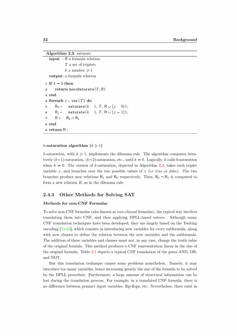
32 Background
Algorithm 2.3: saturateinput : R a formula relation
T a set of tripletsk a number ¥ 1
output: a formula relation
if k 0 then1
return zeroSaturate(T,R)2
end3
foreach x P var(T) do4
R0 ÐÝ saturate(k 1, T, RY tx 0u);5
R1 ÐÝ saturate(k 1, T, RY tx 1u);6
RÐÝ R0 X R17
end8
return R ;9
k-saturation algorithm (k ¥ 1)
k-saturation, with k ¥ 1, implements the dilemma rule. The algorithm computes itera-tively (k1)-saturation, (k2)-saturation, etc., until k 0. Logically, it calls 0-saturationwhen k 0. The version of k-saturation, depicted in Algorithm 2.3, takes each tripletvariable x, and branches over the two possible values of x (i.e true or false). The twobranches produce new relations R1 and R0 respectively. Then, R0 X R1 is computed toform a new relation R, as in the dilemma rule.
2.4.3 Other Methods for Solving SAT
Methods for non-CNF Formulas
To solve non-CNF formulas (also known as non-clausal formulas), the typical way involvestranslating them into CNF, and then applying DPLL-based solvers. Although manyCNF translation techniques have been developed, they are largely based on the Tseitingencoding [Tse83], which consists in introducing new variables for every subformula, alongwith new clauses to define the relation between the new variables and the subformula.The addition of these variables and clauses must not, in any case, change the truth valueof the original formula. This method produces a CNF representation linear in the size ofthe original formula. Table 2.1 depicts a typical CNF translation of the gates AND, OR,and NOT.
But this translation technique causes some problems nonetheless. Namely, it mayintroduce too many variables, hence increasing greatly the size of the formula to be solvedby the DPLL procedure. Furthermore, a large amount of structural information can belost during the translation process. For example, in a translated CNF formula, there isno difference between primary input variables, flip-flops, etc. Nevertheless, there exist in
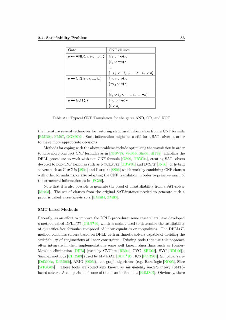
2.4. Satisfiability Problem 33
Gate CNF clauses
oÐ ANDpi1, i2, ..., inq pi1 _ oq^
pi2 _ oq^
...
p i1 _ i2 _ ..._ in _ oq
oÐ ORpi1, i2, ..., inq p i1 _ oq^
p i2 _ oq^
...
pi1 _ i2 _ ..._ in _ oq
oÐ NOTpiq p i_ oq^
pi_ oq
Table 2.1: Typical CNF Translation for the gates AND, OR, and NOT
the literature several techniques for restoring structural information from a CNF formula[RMB04, FM07, OGMS02]. Such information might be useful for a SAT solver in orderto make more appropriate decisions.
Methods for coping with the above problems include optimizing the translation in orderto have more compact CNF formulas as in [NRW98, Vel04b, She04, dlT92], adapting theDPLL procedure to work with non-CNF formula [GS99, TBW04], creating SAT solversdevoted to non-CNF formulas such as NoClause [TBW04] and BcSat [JN00], or hybridsolvers such as CirCUs [JS04] and Pueblo [SS06] which work by combining CNF clauseswith other formalisms, or also adapting the CNF translation in order to preserve much ofthe structural information as in [PG86].
Note that it is also possible to generate the proof of unsatisfiability from a SAT-solver[MA03]. The set of clauses from the original SAT-instance needed to generate such aproof is called unsatisfiable core [LMS04, ZM03].
SMT-based Methods
Recently, as an effort to improve the DPLL procedure, some researchers have developeda method called DPLL(T ) [GHN04] which is mainly used to determine the satisfiabilityof quantifier-free formulas composed of linear equalities or inequalities. The DPLL(T )method combines solvers based on DPLL with arithmetic solvers capable of deciding thesatisfiability of conjunctions of linear constraints. Existing tools that use this approachoften integrate in their implementations some well known algorithms such as Fourier-Motzkin elimination [DE73] (used by CVClite [BB04], CVC [SBD02], SVC [BDL96]),Simplex methods [CLRS09] (used by MathSAT [BBC05], ICS [FORS01], Simplics, Yices[DdM06a, DdM06b], ARIO [SS05]), and graph algorithms (e.g. Barcelogic [NO05], Slice[WIGG05]). These tools are collectively known as satisfiability modulo theory (SMT)-based solvers. A comparison of some of them can be found at [BdMS07]. Obviously, there
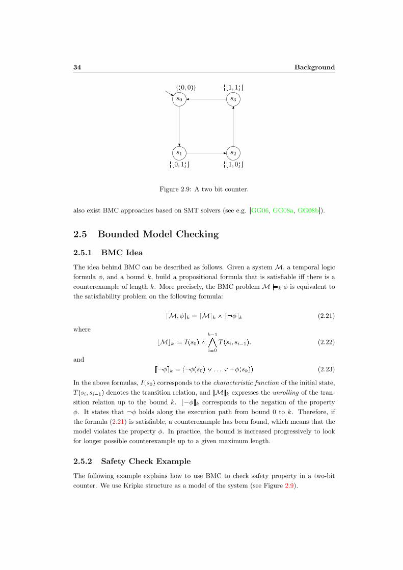
34 Background
s0
tp0, 0qu
s1
tp0, 1qu
s2
tp1, 0qu
s3
tp1, 1qu
Figure 2.9: A two bit counter.
also exist BMC approaches based on SMT solvers (see e.g. [GG06, GG08a, GG08b]).
2.5 Bounded Model Checking
2.5.1 BMC Idea
The idea behind BMC can be described as follows. Given a system M, a temporal logicformula φ, and a bound k, build a propositional formula that is satisfiable iff there is acounterexample of length k. More precisely, the BMC problem M |ùk φ is equivalent tothe satisfiability problem on the following formula:
vM, φwk vMwk ^ v φwk (2.21)
where
vMwk Ips0q ^k1©i0
T psi, si1q. (2.22)
andv φwk p φps0q _ . . ._ φpskqq (2.23)
In the above formulas, Ips0q corresponds to the characteristic function of the initial state,T psi, si1q denotes the transition relation, and vMwk expresses the unrolling of the tran-sition relation up to the bound k. v φwk corresponds to the negation of the propertyφ. It states that φ holds along the execution path from bound 0 to k. Therefore, ifthe formula (2.21) is satisfiable, a counterexample has been found, which means that themodel violates the property φ. In practice, the bound is increased progressively to lookfor longer possible counterexample up to a given maximum length.
2.5.2 Safety Check Example
The following example explains how to use BMC to check safety property in a two-bitcounter. We use Kripke structure as a model of the system (see Figure 2.9).
2.5. Bounded Model Checking 35
Let pa, bq be the Boolean variables that represent the value of bits at each state. Theinitial state and the transition relation are given as follows:
- initial state IpS0q : p a0 ^ b0q,
- transition relation T psi, si1q : pai1 pai biq ^ bi1 biq.
The safety property to be checked is φ AGp a _ bq, which means “it is alwaystrue that either of the two bits is false (or 0).” To determine whether a counterexampleexists, we are more concerned with the negation of φ, that is EF pa^ bq, which means “itis possible to reach a state where both bits are true (or 1).”
By applying the equations (2.22), (2.21), and (2.23) for k 2, we obtain the following:
vM, φw2 IpS0q ^ T ps0, s1q ^ T ps1, s2q ^ v φw2
that is,
vM, φw2 p a0 ^ b0q^
pa1 pa0 b0q ^ b1 b0q^
pa2 pa1 b1q ^ b2 b1q^
ppa0 ^ b0q _ pa1 ^ b1q _ pa2 ^ b2qq.
The formula vM,φw2 is unsatisfiable. Thus, unrolling the transition relation up tok 2 provides no counterexample. On the other hand, if we continue with k 3, wecould see that vM,φw3 provides a satisfiable formula that violates the safety property.
2.5.3 BMC and Liveness Properties
While it is straightforward to check safety properties with BMC (see e.g.[PICW04]), live-ness properties are quite complicated. For example, to check whether the liveness propertyAG EFP holds, we need to verify that all paths from the initial state lead to P . This istypically done in the following way: first, check if a state satisfying P can be reachedwithin bound 1. If yes, then P does not hold in all existing paths within bound 1, thuswe need to increase the bound to 2. We continue the process for bound 2 while assertingthat P holds for bound 1. If we still find a state satisfying P in bound 2, we can keepgoing by increasing the bound. However, if we obtain an unsatisfaiable assignment at anygiven bound, we can conclude that the liveness property holds. More details on how touse BMC for checking liveness properties can be found in [BCCZ99, GGA05].
Note that, when Biere et al. first presented the BMC idea in [BCCZ99], they usedKripke structures to model their system. Subsequent works on BMC adopt alternativemodeling techniques. Still, the idea which underlies these works remains the same asthe original one. For instance, timed automata is used in [WZP03, Sor02], Petri nets in[Hel01, WLP04], and transition systems in [JHN03, Jus04]. As mentioned before, we willalso use transition systems in this work.


Chapter 3
Exixting Techniques
At first, research on BMC was largely revolved around synchronous systems. The charac-teristic of these systems, in which all variables change their values simultaneously, matchesperfectly a BMC operation. More recently, however, a great deal of work on BMC forasynchronous systems has been published. In this chapter we will review some of themost interesting BMC techniques that exist in the literature. Analyses and comparisonsof most of these techniques can be found in [PBG05, AKMM03, ADA05]. We will alsodiscuss briefly how to deal with the completeness issue, and how to combine SAT withunbounded model checking.
3.1 Standard Methods
In general, all BMC techniques fall into two categories: (i) techniques related to theSAT solving and (ii) techniques related to the BMC process itself. The goal, though, isalways the same in every technique: to find a counterexample as fast as possible, if itexists. These techniques include reduction of the BMC problem into another problem,tuning SAT solvers for BMC, learning and preprocessing, incremental SAT solving, andstrengthening and encodings of properties.
Reduction to Another Problem Some techniques consist in reducing the BMC prob-lem into a different kind of problem. For instance, the technique in [HN01a, HN01b] usethe logic programming known as answer set programming [MT99] to reduce the BMCproblem for 1-safe Petri nets into computation of stable models of logic programs. An-other approach for 1-safe Petri nets, introduced in [Hel01], consists in reducing the probleminto Boolean circuit satisfiability checking, using three semantics known as process, step,and interleaving semantics. In [ACKS02], BMC has been applied to timed system. Inthis technique the BMC problem is reduced into satisfiability problem of a math-formulas,that is a Boolean combination of propositional variables and linear mathematical relationsover real variables.
38 Exixting Techniques
Tuning SAT Solvers for BMC Other researches focus on modifying some featuresin the SAT solvers to match the requirements of a BMC operation [Sht00, JAS04, SZ03].These solvers are mainly based on the DPLL algorithm, which solves a formula bytraversing a search tree as described in Section 2.4.1. The structure of a BMC for-mula makes it possible to use alternative branching methodologies during the traversal[WJHS04, Zar04], or to extend the default algorithm so that more conflict clauses can beadded [Sht00, Str04]. In addition, the formulas can be simplified using different methodssuch as the ones in [Kue04, Vel04a] before feeding them to the solvers. These techniquesenable the solvers to speed their execution. Therefore, the performance of BMC usingthem will also improve.
Learning and Preprocessing Using learning mechanisms to extract information froma circuit can improve both SAT solving and BMC. For example, [CNQ03, GGW03] addsome information learned from a BDD-based analysis to the SAT engine to speed itsexecution. The method in [CNQ03] performs first a BDD-based approximate reachabilityanalysis, then converts the BDD at each step into clauses to constrain the SAT solver,whereas the one in [GGW03] extracts clauses dynamically or statically, and limits thelearning process only to local regions to prevent excessive computational and memorycosts.
For every unsatisfiable CNF formula, it is possible to generate a proof of unsatisfiabilityfrom the solver. The set of clauses from the original formula needed for generating sucha proof is called unsatisfiable core. Extracting such information is proven to be usefulespecially in an abstraction-refinement process because it gives an explanation as to whythe formula is unsatisfiable and can guide the refinement. [MA03] suggests a method forgenerating such a proof. [McM03, ZPHS05, GS05, CCK02] show how to use it in BMC.
The authors in [AH04] introduce a preprocessing engine called SIMP2C, which convertsindirect implications learned via logic simulation into constraint clauses. These clausesare replicated throughout the whole BMC run and provided to the SAT solver to speed upits decision process. This reduction technique is also adopted in the Hypre preprocessor[BW03], which, in addition, can perform equality reduction.
The preprocessing engine called NiVER introduced in [SP05] uses a variable elimina-tion technique that does not increase the size of the CNF formula. Though not directlyrelated to clause learning, this technique also improves SAT solving. Hypre and NiVERare designed for general purposed SAT-solver, yet they can also be used for a BMC oper-ation.
Incremental SAT Solving As it turns out, a CNF formula generated at a givenBMC step is, in fact, an extension of the one generated immediately before it. Con-sequently, all propositional formulas obtained during a BMC operation maintain thesame structure. Many SAT solvers exploit this feature to perform incremental solving[Een03, JS05, ZPH04, WKS01, Str01]. That is, the possibility of reusing some conflictclauses learned during one SAT check when solving the next instance. These learned
3.2. Completeness 39
clauses prevent the solver from examining some regions in the search space that containno solution. As a result, the solving speed improves, and so does the entire BMC oper-ation. BMC encodings, built especially for incremental SAT such as the one in [HJL05],will improve even more the whole process. The authors in [JS05] use a general crite-rion for filtering the clauses to be reused, and a distillation technique for preventing theexploration of unneeded regions in the search space.
Property Strengthening While incremental learning can improve the speed of SATsolving, it does not reduce the depth needed to prove a property. On the other hand,property strengthening allows a property to be falsified or verified within small depth. Itdoes so, by enlarging the property so that a counterexample can be detected at an earlierdepth. For example, the framework for proving a property via structural analysis, intro-duced in [BKA02], combines a BDD-based backward unfolding with a target enlargementmechanism in order to make unreachability proof much more easier. It computes first anoverapproximation of the so-called system diameter. Then, performs a mix SAT-basedforward unfolding and the BDD-based backward one from the target states. In [dMRS03],Moura et al. strengthen the property by adding to it a counterexample generated froma failed induction step. In this BMC-induction combination, the strengthening powerdepends largely on the generated counterexample.
Encodings of Properties It is also possible to improve the performance of BMCby finding a better way to encode the properties. For LTL properties, some meth-ods use encodings that allow direct translation of the formula into propositional for-mula [CPRS02, LBHJ04], while others encode the LTL property using Büchi automata[dMRS02, CKOS04]. Some works also deal with CTL properties such as the ones pre-sented in [PWZ02a, PWZ02b].
3.2 Completeness
Numerous techniques have been developed so far in order to make BMC complete, thatis, allowing it not only to look for a counterexample, but also to provide a “yes” or “no”answer, just as in standard model checking (see Figure 1.1). These techniques includecomputing the completeness threshold, temporal induction, interpolation, ATPG-basedmethod, and abstraction.
Computing the Completeness Threshold The idea consists in computing the valueof a bound known as completeness threshold [CKOS04] or also termination length [AS06],within which a counterexample is expected to be found, if it exists. However, computingthis bound is not trivial. Furthermore, its value depends on the property, the model, andthe termination criterion. For reachability properties, for example, completeness thresholdcoincides with the system diameter [BCCZ99, BK04] which is the longest shortest path
40 Exixting Techniques
between two states. Thus, to check whether these properties hold, it is enough to increasethe bound up to the system diameter, and if no counterexample appears within thislimit, then the system is correct. But determining the diameter is no easy task, and itsvalue can be too large to handle. For this reason, Biere et al. propose in [BCCZ99] anoverapproximation called recurrence diameter which corresponds to the longest loop-freepath between two states. This number, while big, is proven to be much easier to computethan the diameter [KS03].
Temporal Induction Here, the goal is to prove the following two conditions whichconstitute the base case and the induction step respectively. Given a bound k, (i) theproperty holds in all paths of length k from the initial states and (ii) for any path oflength k where the property holds in all states, it is not possible from the last stateof the path to reach a state where the property does not hold. In addition, to ensurecompleteness, all states of the paths in the base condition must be distinct [SSS00, Een03].Induction algorithms increase the value of k until the two conditions above are proven ora counterexample is found.
Interpolation An interpolant for the pair pA,Bq is a formula P such that (i) A ñ P
(ii) P ^B is unsatisfiable and (iii) P refers only to the common variables of A and B.If a BMC formula is unsatisfiable, it can be partitioned into conjunction of two for-
mulas A and B, such that A represents the initial states with the first transition, whereasB encodes the rest of the transition up to an initial bound k along with the property.In [McM03, McM05] McMillan introduces an algorithm that computes the interpolant ofthese two formulas. This interpolant corresponds to an overapproximation of the set ofstates reachable from an initial state in one step. Using this interpolant, McMillan’s algo-rithm can determine whether a fixpoint is reached at bound k, or a real counterexampleoccurs. If it reaches a fixpoint, then the property holds and the algorithm stops. If noreal counterexample appears, the algorithm increases the value of k until either it finds areal counterexample or reaches the system diameter. If it reaches the diameter withoutfinding a real counterexample, then the system is correct.
ATPG-based Method In [IPC03], Iyer et al. suggest a quite different approach basedon the technique known as automated test pattern generation (ATPG). Their algorithmperforms an ATPG-based backtracking traversal from states where the property is false.If it reaches an initial state during the traversal, then it generates a counterexample.Otherwise, the property is proven to be true and the algorithm stops. To guaranteecompleteness, it uses additional Boolean constraints to mark already visited states, thusavoiding searching them again in future iterations.
Abstraction Completeness can also be achieved through abstraction-refinement tech-niques, most of which use the unsatisfiable core to refine the model. The algorithm in
3.3. SAT with Unbounded Model Checking 41
[CCK02], for example, starts with an initial abstraction of the model. Using a BDD-based procedure, it checks first whether the property holds in the abstract model. If yes,then the system is correct. Otherwise, it runs a BMC session on the concrete model,taking the length of the abstract counterexample as a BMC length. If the BMC op-eration still returns a counterexample, then the system is incorrect. Otherwise, it usesthe unsatisfiable core to refine the abstract model and restart again with the BDD-basedprocedure.
The proof-based method introduced in [MA03], on the other hand, starts with a BMCsession with an initial length k. If the formula is unsatisfiable, the algorithm uses theunsatisfiable core to create a new abstraction of the model. Then, it runs a standardBDD-based model checker on the abstract model to determine whether it is correct ornot. If it is correct, the algorithm terminates. Otherwise, the BDD-based model checkerproduces a counterexample whose length k1, which is always greater than k, is used lateron as the next BMC bound.
The algorithm in [Kro05] creates an abstraction by using a method known as cut-pointinsertion. That is, it removes some parts of the design and replaces them with nonde-terministically chosen inputs. The result is an abstract model that overapproximates theconcrete one, and preserves safety properties. This algorithm also uses the unsatisfiablecore to refine the model, and to ensure completeness, it can identify reasonably smallcompleteness threshold.
3.3 SAT with Unbounded Model Checking
Adapting SAT to work with unbounded model checking (UMC) makes the image compu-tation process more tractable. SAT-based UMC performs the image computation usingall-solution SAT-solvers. That is, solvers that compute all satisfying solutions (see e.g.[LHS04]), as opposed to general-purposed SAT-solvers which provide only a single solu-tion if it exists. In contrast to BDD-based approaches, this technique stores the set ofreached states as set of clauses, and adds some Blocking clauses in order to avoid reachingthe same solution space in the future. The clauses generated at each iteration can be usedas the starting states for the next iteration.
For example, [GYA01] exploits the strengths of both SAT and BDDs in order toimprove the image computation during a model checking operation. This is achieved bydecomposing first the image computation problem into many sub-problems using a SAT-based algorithm. Each of these sub-problems is handled later on by a conventional BDDapproach. This allows the state space to be represented as BDDs, and the transitionrelation as a CNF formula. The same authors also introduce in [GYAG00] a CNF parti-tioning technique which, combined with the previous method, improves the efficiency ofthe associated SAT algorithm. In [CCK03], Chauchan et. al show how to perform animage computation with a pure SAT procedure. Unlike the method in [GYA01], theyuse clausal form to represent both the state space and the transition relation.
42 Exixting Techniques
The method in [ABE00, BC00], on the other hand, adapts existing BDD-based algo-rithms to work with SAT-solvers. This adaptation increases the class of systems that canbe verified using traditional symbolic methods. In [GGA04], the main purpose is to usesome special features from SAT-based algorithm for tackling the quantifier eliminationproblem, which is one of the most important operations in symbolic model checking.
SAT procedure is also used in [Cla02] to determine whether a counterexample obtainedfrom an abstract model is real or spurious. In case the counterexample is spurious,the algorithm refines the model using integer linear programming and machine learningtechniques.
3.4 Existing BMC Tools
Many BMC-related tools have been developed so far. While some of them are builtespecially to perform BMC operation, others can also handle BDD-based model checking.The most widely used is the one called NuSmv [CCGR99] which has incorporated BMCimplementation since its version 2.0. This tool uses reduced Boolean circuits [ABE00] asan intermediate representation for the propositional formulas.
The BMC feature has also been included in Vis [BHSV96] since its version 2.0.Unlike NuSmv, it does not use intermediate representation for generating formulas.
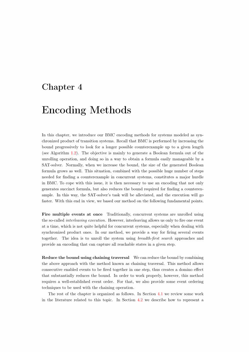
Chapter 4
Encoding Methods
In this chapter, we introduce our BMC encoding methods for systems modeled as syn-chronized product of transition systems. Recall that BMC is performed by increasing thebound progressively to look for a longer possible counterexample up to a given length(see Algorithm 1.2). The objective is mainly to generate a Boolean formula out of theunrolling operation, and doing so in a way to obtain a formula easily manageable by aSAT-solver. Normally, when we increase the bound, the size of the generated Booleanformula grows as well. This situation, combined with the possible huge number of stepsneeded for finding a counterexample in concurrent systems, constitutes a major hurdlein BMC. To cope with this issue, it is then necessary to use an encoding that not onlygenerates succinct formula, but also reduces the bound required for finding a counterex-ample. In this way, the SAT-solver’s task will be alleviated, and the execution will gofaster. With this end in view, we based our method on the following fundamental points.
Fire multiple events at once Traditionally, concurrent systems are unrolled usingthe so-called interleaving execution. However, interleaving allows us only to fire one eventat a time, which is not quite helpful for concurrent systems, especially when dealing withsynchronized product ones. In our method, we provide a way for firing several eventstogether. The idea is to unroll the system using breadth-first search approaches andprovide an encoding that can capture all reachable states in a given step.
Reduce the bound using chaining traversal We can reduce the bound by combiningthe above approach with the method known as chaining traversal. This method allowsconsecutive enabled events to be fired together in one step, thus creates a domino effectthat substantially reduces the bound. In order to work properly, however, this methodrequires a well-established event order. For that, we also provide some event orderingtechniques to be used with the chaining operation.
The rest of the chapter is organized as follows. In Section 4.1 we review some workin the literature related to this topic. In Section 4.2 we describe how to represent a
44 Encoding Methods
transition system symbolically. In Section 4.3 we introduce a BMC encoding devotedfor single independent systems. In Section 4.4 we detail the encoding for synchronizedtransition systems. In Section 4.5 we show how to express reachability properties. Weend the Chapter with the chaining method in Section 4.6.
4.1 Related Work
We will now review some BMC encodings in the literature related to asynchronous con-current systems. In [Jus04, JHN03] Jussila et al. introduce a BMC technique for systemsmodeled as labeled transition systems (LTSs). Their idea consists in translating LTSs intoBoolean formula using some predefined translation predicates. This technique allows sev-eral independent actions to happen simultaneously. As a result, it can shorten the boundneeded to detect a property violation. The encoding in [Hel01] also adopts a similar ideafor Petri net models. It uses some translation rules to obtain a Boolean circuit (BC)from the unrolling operation, and uses a BC-based solver to check the satisfiability of thegenerated circuit. By using translation rules, as in the above approaches, the Booleanformula is not constructed directly from the model itself. Instead, it is derived from thenewly obtained representation after applying the rules.
By contrast, the methods in [OTK04] and [Sor02], which apply to Petri nets andtimed automata respectively, derive the Boolean formula directly from the definition ofthe system itself rather than relying on transformation rules. In addition, the authors of[Sor02] show how to make BMC for timed automata complete by setting up a lower and anupper bounds for the length k of counterexample. On the other hand, while the methodin [OTK04] has produced interesting results, its performance depends on a preprocessingalgorithm that computes a total order of the transitions.
In [GG08b], Ganai et al. apply BMC to multi-thread concurrent systems with sharedmemory, such as multi-processor computers. They use their method to check safety prop-erties such as data races for these types of systems, which they model using extendedfinite state machine (EFSM). In their approach, they first create independent models foreach individual thread in the system, then, to ensure synchronization, explicitly add addi-tional synchronization constraints into the model. To reduce the size of these constraintsthey do not allow local wait cycles (i.e. there are no self-loops in local read/write blockswith shared accesses.) They also transform the model using some property preservingtechniques, which further reduce the size of concurrency constraints. They check thesatisfiability of the generated formula with SMT-based solver instead of a standard one.
The methods most closely related to ours are the ones introduced in [Jus04, JHN03],which also deal with synchronized product of transition systems. However, the principlesare quite different since, in our work, we do not use transformation rules. The methodin [OTK04], while using direct transformation, differs from ours in the type of system towhich it applies—Petri net vs. transition system. The method in [Sor02] also use directtransformation but it is for timed systems.
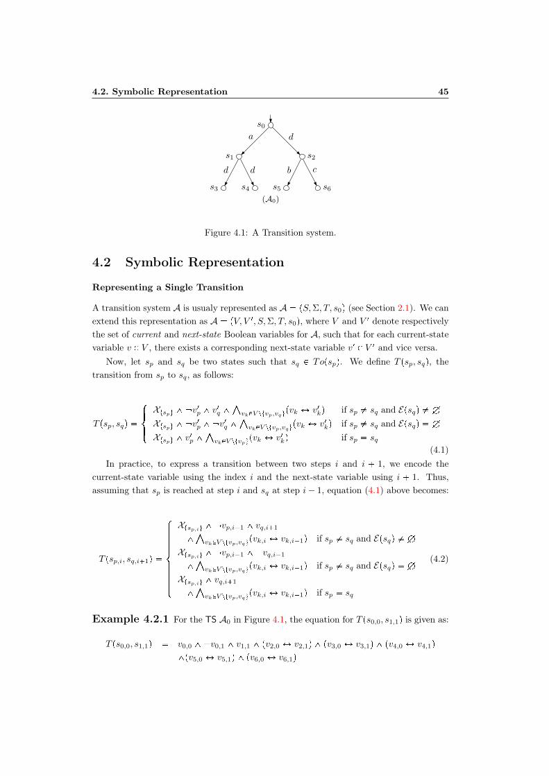
4.2. Symbolic Representation 45
s0
s1 s2
s3 s4 s5 s6
(A0)
a
d bd
d
c
Figure 4.1: A Transition system.
4.2 Symbolic Representation
Representing a Single Transition
A transition system A is usualy represented as A pS,Σ, T, s0q (see Section 2.1). We canextend this representation as A pV, V 1, S,Σ, T, s0q, where V and V 1 denote respectivelythe set of current and next-state Boolean variables for A, such that for each current-statevariable v P V , there exists a corresponding next-state variable v1 P V 1 and vice versa.
Now, let sp and sq be two states such that sq P Topspq. We define T psp, sqq, thetransition from sp to sq, as follows:
T psp, sqq
$'&'%
Xtspu ^ v1p ^ v1q ^vkPV ztvp,vqu
pvk Ø v1kq if sp sq and Epsqq HXtspu ^ v1p ^ v1q ^
vkPV ztvp,vqu
pvk Ø v1kq if sp sq and Epsqq HXtspu ^ v1p ^
vkPV ztvpu
pvk Ø v1kq if sp sq(4.1)
In practice, to express a transition between two steps i and i 1, we encode thecurrent-state variable using the index i and the next-state variable using i 1. Thus,assuming that sp is reached at step i and sq at step i 1, equation (4.1) above becomes:
T psp,i, sq,i1q
$''''''''&''''''''%
Xtsp,iu ^ vp,i1 ^ vq,i1
^vkPV ztvp,vqu
pvk,i Ø vk,i1q if sp sq and Epsqq HXtsp,iu ^ vp,i1 ^ vq,i1
^vkPV ztvp,vqu
pvk,i Ø vk,i1q if sp sq and Epsqq HXtsp,iu ^ vq,i1
^vkPV ztvp,vqu
pvk,i Ø vk,i1q if sp sq
(4.2)
Example 4.2.1 For the TS A0 in Figure 4.1, the equation for T ps0,0, s1,1q is given as:
T ps0,0, s1,1q v0,0 ^ v0,1 ^ v1,1 ^ pv2,0 Ø v2,1q ^ pv3,0 Ø v3,1q ^ pv4,0 Ø v4,1q
^pv5,0 Ø v5,1q ^ pv6,0 Ø v6,1q

46 Encoding Methods
Representing Multiple Transitions
Given two sets of states Sp and Sq such that TopSpq Sq. Assume Sp is reached at stepi and Sq at step i 1. To capture the execution of multiple transitions together from Sp,we define T pSp,i, Sq,i1q as follows:
T pSp,i, Sq,i1q ©
spPSp;sqPSq
T psp,i, sq,i1q (4.3)
Equation 4.3 is useful for capturing the firing of multiple events together from thestates where they are enabled.
Example 4.2.2 For the TS A0, assume that at step 0, we start with S0 ts0u, andat step 1 we reach S1 ts1, s2u. Then T pS0,0, S1,1q is given as:
T pS0,0, S1,1q v0,0 ^ v0,1 ^ v1,1 ^ v2,1 ^ pv3,0 Ø v3,1q ^ pv4,0 Ø v4,1q
^pv5,0 Ø v5,1q ^ pv6,0 Ø v6,1q
Note that, the example above may appear incomplete as it concerns only a transitionbetween two consecutive steps as described in equation (4.3). We will see in the nextsection how to encode a complete BMC execution starting from the initial state up to agiven bound.
4.3 Encoding for Independent Systems
In this section, we will discuss how to encode a BMC operation for a single independentTS. We will start with the standard interleaving execution, and continue with a methodbased on the so-called breadth-first search.
4.3.1 Interleaving Execution
Introduction
To capture the behavior of concurrent systems it is not uncommon to use the methodknown as interleaving execution [CGP99], which allows only one event, within one tran-sition, to fire at each step. As a result, with this technique, we can reach at most onesingle state at each step, and can only obtain an execution path formed by succession ofsingle transitions from bound 0 to k. The events in this path follow a linear order knownas interleaving sequence.
Application to BMC
Given a TS A pS,Σ, T, s0q, a property φ, and a bound k. The BMC formula for A,defined in terms of interleaving execution, is given as
intvA, φwk intvAwk ^ v φwk (4.4)

4.3. Encoding for Independent Systems 47
where
- intvAwk defines the unrolling of A up to bound k using interleaving execution, i.e.
intvAwk Ips0q ^k1©i0
T psi, si1q (4.5)
- Ips0q denotes the characteristic function of the initial state, and is defined as
Ips0q Xts0,0u ^©sps0
vp,0 (4.6)
- T psi, si1q T psp,i, sq,i1q such that sp is a state reached at step i, and sq is onereached at step i 1.
- v φwk corresponds to the negation of the property at bound k.
For the moment we are only interested in the unrolling part of the BMC formula.Hence, we will not detail v φwk until Section 4.5.
Example 4.3.1 For the system A0 in Figure 4.1 we can obtain the following inter-leaving execution for bound k 2
intvAw2 Ips0q
^T ps0,0, s1,1q
^T ps1,1, s4,2q
v0,0 ^ v1,0 ^ v2,0 ^ v3,0 ^ v4,0 ^ v5,0 ^ v6,0
^v0,0 ^ v0,1 ^ v1,1 ^ pv2,0 Ø v2,1q ^ pv3,0 Ø v3,1q
^pv4,0 Ø v4,1q ^ pv5,0 Ø v5,1q ^ pv6,0 Ø v6,1q
^v1,1 ^ v1,2 ^ v4,2 ^ pv2,1 Ø v2,2q ^ pv3,1 Ø v3,2q
^pv5,1 Ø v5,2q ^ pv6,1 Ø v6,2q ^ pv0,1 Ø v0,2q
Theorem 4.3.1Given a transition system A, a property φ, and a bound k. If intvA, φwk is satisfiable,then A * φ.
Proof Assume that intvA, φwk is satisfiable. From the equation (4.5) we have T psi, si1q
1 iff si1 is reachable from si in one step. Obviously, this implies that T ps0, s1q ^ . . . ^
T psk1, skq 1 iff s0, . . . , sk represents a run from the initial state. Since intvA, φwk Ips0q ^ T ps0, s1q ^ . . . ^ T psk1, skq ^ v φwk is satisfiable, we can conclude that a stateviolating the property φ is reachable in k steps or less from the initial state.
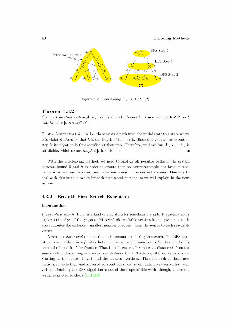
48 Encoding Methods
Interleaving pathss0
s1 s2
s3 s4 s5 s6
p1q
a
d bd
d
c
BFS Step 0
BFS Step 1
BFS Step 2
s0
s1 s2
s3 s4 s5 s6
p2q
a
d bd
d
c
Figure 4.2: Interleaving (1) vs. BFS. (2)
Theorem 4.3.2Given a transition system A, a property φ, and a bound k. A * φ implies Dk P N suchthat intvA, φwk is satisfiable.
Proof Assume that A * φ, i.e. there exists a path from the initial state to a state whereφ is violated. Assume that k is the length of that path. Since φ is violated at executionstep k, its negation is thus satisfied at that step. Therefore, we have intvAwk ^ v φwk issatisfiable, which means intvA, φwk is satisfiable.
With the interleaving method, we need to analyze all possible paths in the systembetween bound 0 and k in order to ensure that no counterexample has been missed.Doing so is onerous, however, and time-consuming for concurrent systems. One way todeal with this issue is to use breadth-first search method as we will explain in the nextsection.
4.3.2 Breadth-First Search Execution
Introduction
Breadth-first search (BFS) is a kind of algorithm for searching a graph. It systematicallyexplores the edges of the graph to “discover” all reachable vertices from a given source. Italso computes the distance—smallest number of edges—from the source to each reachablevertex.
A vertex is discovered the first time it is encountered during the search. The BFS algo-rithm expands the search frontier between discovered and undiscovered vertices uniformlyacross the breadth of the frontier. That is, it discovers all vertices at distance k from thesource before discovering any vertices at distance k 1. To do so, BFS works as follows.Starting at the source, it visits all the adjacent vertices. Then for each of those newvertices, it visits their undiscovered adjacent ones, and so on, until every vertex has beenvisited. Detailing the BFS algorithm is out of the scope of this work, though. Interestedreader is invited to check [CLRS09].
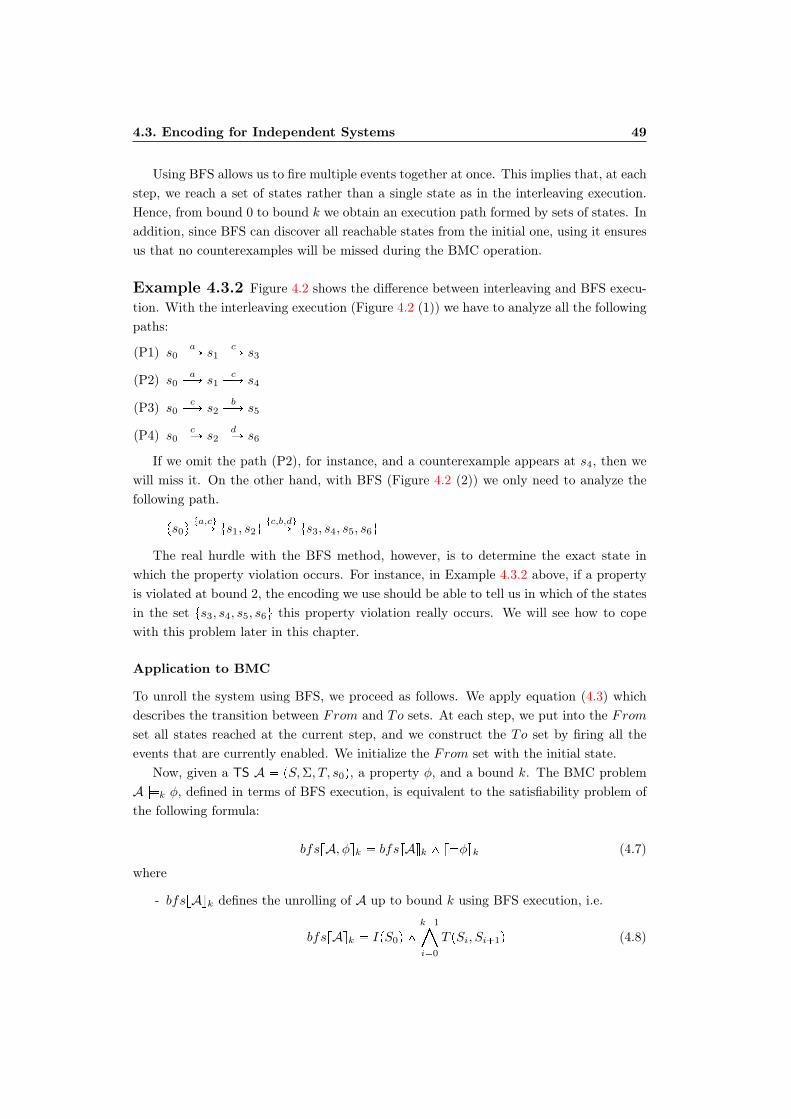
4.3. Encoding for Independent Systems 49
Using BFS allows us to fire multiple events together at once. This implies that, at eachstep, we reach a set of states rather than a single state as in the interleaving execution.Hence, from bound 0 to bound k we obtain an execution path formed by sets of states. Inaddition, since BFS can discover all reachable states from the initial one, using it ensuresus that no counterexamples will be missed during the BMC operation.
Example 4.3.2 Figure 4.2 shows the difference between interleaving and BFS execu-tion. With the interleaving execution (Figure 4.2 (1)) we have to analyze all the followingpaths:
(P1) s0aÝÑ s1
cÝÑ s3
(P2) s0aÝÑ s1
cÝÑ s4
(P3) s0cÝÑ s2
bÝÑ s5
(P4) s0cÝÑ s2
dÝÑ s6
If we omit the path (P2), for instance, and a counterexample appears at s4, then wewill miss it. On the other hand, with BFS (Figure 4.2 (2)) we only need to analyze thefollowing path.
ts0uta,cuÝÑ ts1, s2u
tc,b,duÝÑ ts3, s4, s5, s6u
The real hurdle with the BFS method, however, is to determine the exact state inwhich the property violation occurs. For instance, in Example 4.3.2 above, if a propertyis violated at bound 2, the encoding we use should be able to tell us in which of the statesin the set ts3, s4, s5, s6u this property violation really occurs. We will see how to copewith this problem later in this chapter.
Application to BMC
To unroll the system using BFS, we proceed as follows. We apply equation (4.3) whichdescribes the transition between From and To sets. At each step, we put into the Fromset all states reached at the current step, and we construct the To set by firing all theevents that are currently enabled. We initialize the From set with the initial state.
Now, given a TS A pS,Σ, T, s0q, a property φ, and a bound k. The BMC problemA |ùk φ, defined in terms of BFS execution, is equivalent to the satisfiability problem ofthe following formula:
bfsvA, φwk bfsvAwk ^ v φwk (4.7)
where
- bfsvAwk defines the unrolling of A up to bound k using BFS execution, i.e.
bfsvAwk IpS0q ^k1©i0
T pSi, Si1q (4.8)
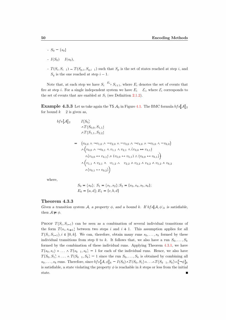
50 Encoding Methods
- S0 ts0u
- IpS0q Ips0q,
- T pSi, Si1q T pSp,i, Sq,i1q such that Sp is the set of states reached at step i, andSq is the one reached at step i 1.
Note that, at each step we have SiEiÝÑ Si1, where Ei denotes the set of events that
fire at step i. For a single independent system we have Ei Ei, where Ei corresponds tothe set of events that are enabled at Si (see Definition 2.1.2).
Example 4.3.3 Let us take again the TS A0 in Figure 4.1. The BMC formula bfsvAw2for bound k 2 is given as,
bfsvAw2 IpS0q
^T pS0,0, S1,1q
^T pS1,1, S2,2q
v0,0 ^ v1,0 ^ v2,0 ^ v3,0 ^ v4,0 ^ v5,0 ^ v6,0
^v0,0 ^ v0,1 ^ v1,1 ^ v2,1 ^ pv3,0 Ø v3,1q
^pv4,0 Ø v4,1q ^ pv5,0 Ø v5,1q ^ pv6,0 Ø v6,1q
^v1,1 ^ v2,1 ^ v1,2 ^ v2,2 ^ v3,2 ^ v4,2 ^ v5,2 ^ v6,2
^pv0,1 Ø v0,2q
where,S0 ts0u; S1 ts1, s2u;S2 ts3, s4, s5, s6u;
E0 ta, du;E1 tc, b, du
Theorem 4.3.3Given a transition system A, a property φ, and a bound k. If bfsvA, φwk is satisfiable,then A * φ.
Proof T pSi, Si1q can be seen as a combination of several individual transitions ofthe form T psi, si1q between two steps i and i 1. This assumption applies for allT pSi, Si1q, i P r0, ks. We can, therefore, obtain many runs s0, . . . , sk formed by theseindividual transitions from step 0 to k. It follows that, we also have a run S0, . . . , Sk
formed by the combination of these individual runs. Applying Theorem 4.3.1, we haveT ps0, s1q ^ . . . ^ T psk1, skq 1 for each of the individual runs. Hence, we also haveT pS0, S1q ^ . . . ^ T pSk1, Skq 1 since the run S0, . . . , Sk is obtained by combining alls0, . . . , sk runs. Therefore, since bfsvA, φwk IpS0q^T pS0, S1q^. . .^T pSk1, Skq^v φwk
is satisfiable, a state violating the property φ is reachable in k steps or less from the initialstate.
4.4. Encoding for Synchronized Systems 51
Theorem 4.3.4Given a transition system A, a property φ, and a bound k. A * φ implies Dk P N suchthat bfsvA, φwk is satisfiable.
Proof The proof of this theorem is similar to the one for Theorem 4.3.2 except thathere, we are dealing with set of states rather than a single state. Assume that A * φ.This means there exists a reachable set of states containing a state that violates theproperty φ. This set is reached from the initial state through a run formed by all thereachable states at each execution step. Assume k is the length of the run. Since φis violated at step k, its negation is thus satisfied at that step. Therefore, we haveIpS0q ^ T pS0, S1q ^ . . . ^ T pSk1, Skq ^ v φwk is satisfiable, which means bfsvA, φwk issatisfiable.
4.4 Encoding for Synchronized Systems
Asynchronous concurrent systems are composed of many components that communicatebetween each other. We model them using synchronized product of transition systems.The approach in Section 4.3 allows us only to encode the BMC execution of a singlecomponent—considered independent—without taking into account the synchronization.Starting from now on, we will always work on synchronized systems.
In this section, we introduce some encoding methods for these systems. As before, wewill start with the interleaving execution and continue with the BFS one.
4.4.1 Interleaving Execution
Introduction
Let us first start by defining the synchronized product of TSs in terms of interleavingexecution.
Definition 4.4.1 (Synchronized Product of TSs)Let A0, . . . ,Am be TSs. Their synchronized product defined in terms of interleavingexecution, denoted pA0, . . . ,Amq is the TS A pS,Σ, T, s0q such that,
- Aj pSj ,Σj , T j , sj0q, j P r0,ms
- S S0 . . . Sm
- s0 ps00, . . . , s
m0 q
- Σ mj0 Σj ,
- T S Σ S
52 Encoding Methods
The firing of an event at each step i should respect the following synchronization condition:given a transition t pps0
i , . . . , smi q, ei, ps
0i1, . . . , s
mi1qq, for all 0 ¤ j ¤ m if ei P Σj then
psji , ei, sji1q P T
j otherwise sji1 sji . That is, we can fire an event only if it is a localevent—an event that exists only in one component—or it is synchronized, and is enabledin all components that have it in their alphabets. sji denotes the state reached at step ifor component j.
To respect the rules in interleaving execution, we have to fire only one event at eachstep. In addition, each component of the system must execute at most one transitionrelated to the enabled event at a time. However, since we are dealing with synchronizedproduct of TSs, we need to take into account the fact that the event may be enabled inseveral components. Thus, we have to fire it in each of these components to guarantee thesynchronization. All this means that, at each step, we fire only one event, but possibly,many transitions from different components.
Example 4.4.1 In Figure 4.3, we combine the system A0 with another one A1. Wethen obtain a synchronized systemA pA0,A1q. We can obtain the following interleavingexecution for bound k 2:
ps0, s7qaÝÑ ps1, s8q
dÝÑ ps4, s8q
Application to BMC
Now, consider a synchronized TS A pA0, . . . ,Amq, a property φ, and a bound k. Wedefine the BMC formula for A, in terms of interleaving execution, as follows.
IntvA, φwk IntvAwk ^ v φwk (4.9)
where
- IntvAwk defines the unrolling of A up to bound k using interleaving execution, i.e.
IntvAwk IIntps0q ^k1©i0
TIntpsi, si1q (4.10)
- IIntps0q denotes the characteristic function of the initial state, such that
IIntps0q Xts00,...,sm0 u ^©
spPm
j0 Sjzts00,...,s
m0 u
vp,0 (4.11)
- TIntpsi, si1q defines the transition between two steps i and i 1 such that
TIntpsi, si1q T pts0i , . . . , s
mi u, ts
0i1, . . . , s
mi1uq (4.12)
Recall that the firing of an event at each step should respect the synchronizationcriterion given in Definition 4.4.1.
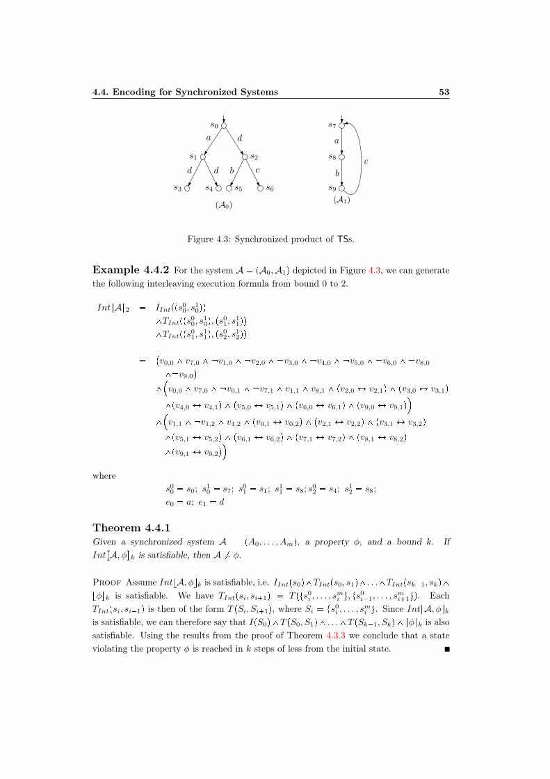
4.4. Encoding for Synchronized Systems 53
s0
s1 s2
s3 s4 s5 s6
(A0)
a
d bd
d
c
s7
s8
s9
(A1)
a
b
c
Figure 4.3: Synchronized product of TSs.
Example 4.4.2 For the system A pA0,A1q depicted in Figure 4.3, we can generatethe following interleaving execution formula from bound 0 to 2.
IntvAw2 IIntpps00, s
10qq
^TIntpps00, s
10q, ps
01, s
11qq
^TIntpps01, s
11q, ps
02, s
12qq
v0,0 ^ v7,0 ^ v1,0 ^ v2,0 ^ v3,0 ^ v4,0 ^ v5,0 ^ v6,0 ^ v8,0
^ v9,0
^v0,0 ^ v7,0 ^ v0,1 ^ v7,1 ^ v1,1 ^ v8,1 ^ pv2,0 Ø v2,1q ^ pv3,0 Ø v3,1q
^pv4,0 Ø v4,1q ^ pv5,0 Ø v5,1q ^ pv6,0 Ø v6,1q ^ pv9,0 Ø v9,1q
^v1,1 ^ v1,2 ^ v4,2 ^ pv0,1 Ø v0,2q ^ pv2,1 Ø v2,2q ^ pv3,1 Ø v3,2q
^pv5,1 Ø v5,2q ^ pv6,1 Ø v6,2q ^ pv7,1 Ø v7,2q ^ pv8,1 Ø v8,2q
^pv9,1 Ø v9,2q
wheres0
0 s0; s10 s7; s0
1 s1; s11 s8; s0
2 s4; s12 s8;
e0 a; e1 d
Theorem 4.4.1Given a synchronized system A pA0, . . . , Amq, a property φ, and a bound k. IfIntvA, φwk is satisfiable, then A * φ.
Proof Assume IntvA, φwk is satisfiable, i.e. IIntps0q^TIntps0, s1q^. . .^TIntpsk1, skq^
vφwk is satisfiable. We have TIntpsi, si1q T pts0i , . . . , s
mi u, ts
0i1, . . . , s
mi1uq. Each
TIntpsi, si1q is then of the form T pSi, Si1q, where Si ts0i , . . . , s
mi u. Since IntvA, φwk
is satisfiable, we can therefore say that IpS0q^T pS0, S1q^ . . .^T pSk1, Skq^vφwk is alsosatisfiable. Using the results from the proof of Theorem 4.3.3 we conclude that a stateviolating the property φ is reached in k steps of less from the initial state.
54 Encoding Methods
Theorem 4.4.2Given a synchronized transition system A, a property φ, and a bound k. A * φ impliesDk P N such that IntvA, φwk is satisfiable.
Proof Assume A * φ is satisfiable. This means there is a path from the initial state toa state violating the property φ. Assume k is the length of that path. In a synchronizedsystem using the interleaving execution, a path of length k is a succession of transitionsTIntpsi, si1q, 0 ¤ i ¤ k 1. Since φ is violated at step k, then its negation is satisfied athat step. Therefore we have IIntps0q^TIntps0, s1q^. . .^TIntpsk1, skq^ φ is satisfiable,i.e. IntvA, φwk is satisfiable.
4.4.2 Breadth-First Search Execution
Introduction
As before, we first start with the definition of synchronized product of TSs in terms ofBFS execution.
Definition 4.4.2Let A0, . . . ,Am be TSs. Their synchronized product, defined in terms of BFS, denotedpA0, . . . ,Amq is the TS A pS,Σ, T, s0q such that,
- Aj pSj ,Σj , T j , sj0q, j P r0,ms,
- S 2S0
. . . 2Sm
,
- s0 pS00 , . . . , S
m0 q, where S
j0 ts
j0u, j P r0,ms,
- Σ mj0 Σj ,
- T S 2Σ S.
The firing of an event at each step i should respect the following synchronizationcondition: given a transition t ppS0
i , . . . , Smi q, Ei, pS
0i1, . . . , S
mi1qq, for all 0 ¤ j ¤ m
if Dei P Ei such that ei P Σj then Dpsji , ei, sji1q P T
j such that sji P Sji and sji1 P S
ji1
otherwise Sji1 Sji . That is, we can fire an event only if it is a local event—an event thatexists only in one component—or it is synchronized, and is enabled in all components thathave it in their alphabets. Sji denotes the set of states reached at step i for component j
The above synchronization condition is similar to the one in Definition 4.4.1, exceptthat here we are firing a set of events rather than a single event. Using BFS allows usto fire not only synchronized events but also independent ones, all together in one step.However, because of the above condition, and unlike the BFS method for independentsystems, not all enabled events could be fired. Once we know the set of fireable events,we fire them using a standard BFS procedure as explained earlier.

4.4. Encoding for Synchronized Systems 55
Example 4.4.3 From the synchronized system A pA0,A1q shown in Figure 4.4 wecan obtain the following BFS execution from bound 0 to 2 (each dashed line in the figurecorresponds to one step):
pS00 , S
10q
E0ÝÑ pS01 , S
11q
E1ÝÑ pS02 , S
12q
where
S00 ts0u; S
10 ts7u; S
01 ts1, s2u; S
11 ts8u;S
02 ts3, s4, s5u; S
12 ts9u;
E0 ta, du; E1 td, bu
Application to BMC
Now, given a synchronized system A pA0, . . . ,Amq, a property φ, and a bound k. Wedefine the BMC formula for A, in terms of BFS execution, as follows.
BfsvA, φwk BfsvAwk ^ v φwk (4.13)
where
- BfsvAwk defines the unrolling of A up to bound k using BFS execution, i.e.
BfsvAwk IBfsps0q ^k1©i0
TBfspsi, si1q (4.14)
- IBfsps0q corresponds to the characteristic of the initial state, such that
IBfsps0q Xmj0 S
j0^
©spPm
j0 Sjzm
j0 Sj0
vp,0 (4.15)
- TBfspsi, si1q defines the transitions between step i and i 1 such that
TBfspsi, si1q T pm¤j0
Sji ,m¤j0
Sji1q (4.16)
Example 4.4.4 To illustrate this representation, let us continue the Example 4.4.3and apply BMC for bound k 2. The formula BfsvAw2 is given as:
BfsvAw2 IBfsppS00 , S
10qq
^TBfsppS00 , S
10q, pS
01 , S
11qq
^TBfsppS01 , S
11q, pS
02 , S
12qq
v0,0 ^ v7,0 ^ v1,0 ^ v2,0 ^ v3,0 ^ v4,0 ^ v5,0 ^ v6,0 ^ v8,0^
v9,0
^v0,0 ^ v7,0 ^ v0,1 ^ v7,1 ^ v1,1 ^ v2,1 ^ v8,1 ^ pv3,0 Ø v3,1q
^pv4,0 Ø v4,1q ^ pv5,0 Ø v5,1q ^ pv6,0 Ø v6,1q ^ pv9,0 Ø v9,1q
^v1,1 ^ v2,1 ^ v8,1 ^ v1,2 ^ v2,2 ^ v8,2 ^ v3,2 ^ v4,2 ^ v5,2
^v9,2 ^ pv0,1 Ø v0,2q ^ pv6,1 Ø v6,2q ^ pv7,1 Ø v7,2q
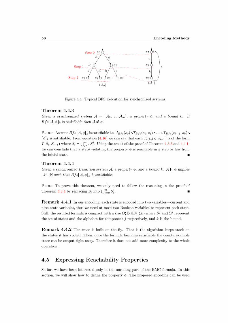
56 Encoding Methods
Step 0
Step 1
Step 2
s0
s1 s2
s3 s4 s5 s6
(A0)
a
d bd
d
c
s7
s8
s9
(A1)
a
b
c
Figure 4.4: Typical BFS execution for synchronized systems.
Theorem 4.4.3Given a synchronized system A pA0, . . . ,Amq, a property φ, and a bound k. IfBfsvA, φwk is satisfiable then A * φ.
Proof AssumeBfsvA, φwk is satisfiable i.e. IBfsps0q^TBfsps0, s1q^. . .^TBfspsk1, skq^
vφwk is satisfiable. From equation (4.16) we can say that each TBfspsi, si1q is of the formT pSi, Si1q where Si
mj0 S
ji . Using the result of the proof of Theorem 4.3.3 and 4.4.1,
we can conclude that a state violating the property φ is reachable in k step or less fromthe initial state.
Theorem 4.4.4Given a synchronized transition system A, a property φ, and a bound k. A * φ impliesDk P N such that BfsvA, φwk is satisfiable.
Proof To prove this theorem, we only need to follow the reasoning in the proof ofTheorem 4.3.4 by replacing Si into
mj0 S
ji .
Remark 4.4.1 In our encoding, each state is encoded into two variables—current andnext-state variables, thus we need at most two Boolean variables to represent each state.Still, the resulted formula is compact with a size OpΣjp|Sj |q.kq where Sj and Σj representthe set of states and the alphabet for component j respectively, and k is the bound.
Remark 4.4.2 The trace is built on the fly. That is the algorithm keeps track onthe states it has visited. Then, once the formula becomes satisfiable the counterexampletrace can be output right away. Therefore it does not add more complexity to the wholeoperation.
4.5 Expressing Reachability Properties
So far, we have been interested only in the unrolling part of the BMC formula. In thissection, we will show how to define the property φ. The proposed encoding can be used
4.5. Expressing Reachability Properties 57
for checking reachability properties, which express that some particular situation can bereached. Checking such properties is equivalent to determining whether there exists anexecution path leading to a state satisfying the property. These properties can be simple,for instance “we can enter a critical section,” or conditional, for instance “we can entera critical section without passing through n 0,” or also in negative form such as “wecannot have n 0.”
In particular, we use our method to check if there is a deadlock in a system, i.e. if thereexists a reachable state with no firing events. Formally, a deadlock run in a transitionsystem is defined as follows.
Definition 4.5.1Let σ s0
e0ÝÑ s1e1ÝÑ . . .
ek1ÝÑ sk be a run of a TS A. σ is a deadlock run iff the state sk
does not have any outgoing transitions.
For synchronized systems, two cases should be considered in order to express deadlockconditions:
- the deadlock state is reached after firing a local event,
- the deadlock state is reached after firing a synchronized event and each synchronizedcounterpart of that event also reaches a deadlock state.
Let R be the set of reachable states for all components at a given bound k. R canbe divided into two subset Rl and Rs which correspond to the states reached by localevents and the synchronized ones respectively. Rs can still be divided into several subsetsL1, . . . , Ln such that each Li contains states reached by related events—i.e. events withtheir synchronized counterparts.
The deadlock condition for a system can be expressed by the negation of the following“live” condition, which expresses that at each step we can always fire some events fromeach reachable state:
vLivewk ©siPRl
vi,k ^©LRs
ªsjPL
vj,k
(4.17)
The negation of the property above expresses that we can obtain a reachable state withno firing events, which means a deadlock appears in that state. The deadlock conditionat a bound k is thus given as follow:
v Livewk ©siPRl
vi,k ^©LRs
ªsjPL
vj,k
(4.18)
Example 4.5.1 Let us take again our running example depicted in Figure 4.3. Thedeadlock condition for this system at bound 2, using the BFS execution (see Figure 4.4),is given as:
v Livew2 v3,2 ^ v4,2 ^ pv5,2 _ v9,2q
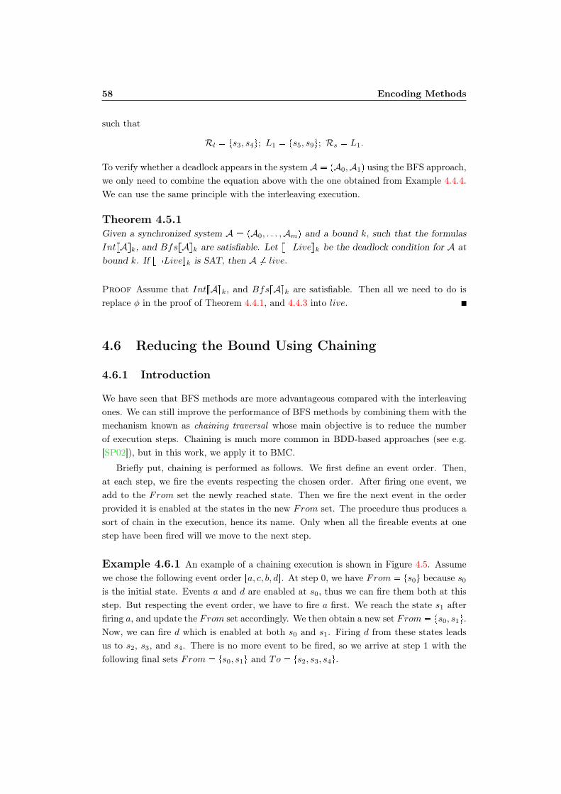
58 Encoding Methods
such that
Rl ts3, s4u; L1 ts5, s9u; Rs L1.
To verify whether a deadlock appears in the systemA pA0,A1q using the BFS approach,we only need to combine the equation above with the one obtained from Example 4.4.4.We can use the same principle with the interleaving execution.
Theorem 4.5.1Given a synchronized system A pA0, . . . ,Amq and a bound k, such that the formulasIntvAwk, and BfsvAwk are satisfiable. Let v Livewk be the deadlock condition for A atbound k. If v Livewk is SAT, then A * live.
Proof Assume that IntvAwk, and BfsvAwk are satisfiable. Then all we need to do isreplace φ in the proof of Theorem 4.4.1, and 4.4.3 into live.
4.6 Reducing the Bound Using Chaining
4.6.1 Introduction
We have seen that BFS methods are more advantageous compared with the interleavingones. We can still improve the performance of BFS methods by combining them with themechanism known as chaining traversal whose main objective is to reduce the numberof execution steps. Chaining is much more common in BDD-based approaches (see e.g.[SP02]), but in this work, we apply it to BMC.
Briefly put, chaining is performed as follows. We first define an event order. Then,at each step, we fire the events respecting the chosen order. After firing one event, weadd to the From set the newly reached state. Then we fire the next event in the orderprovided it is enabled at the states in the new From set. The procedure thus produces asort of chain in the execution, hence its name. Only when all the fireable events at onestep have been fired will we move to the next step.
Example 4.6.1 An example of a chaining execution is shown in Figure 4.5. Assumewe chose the following event order ra, c, b, ds. At step 0, we have From ts0u because s0
is the initial state. Events a and d are enabled at s0, thus we can fire them both at thisstep. But respecting the event order, we have to fire a first. We reach the state s1 afterfiring a, and update the From set accordingly. We then obtain a new set From ts0, s1u.Now, we can fire d which is enabled at both s0 and s1. Firing d from these states leadsus to s2, s3, and s4. There is no more event to be fired, so we arrive at step 1 with thefollowing final sets From ts0, s1u and To ts2, s3, s4u.
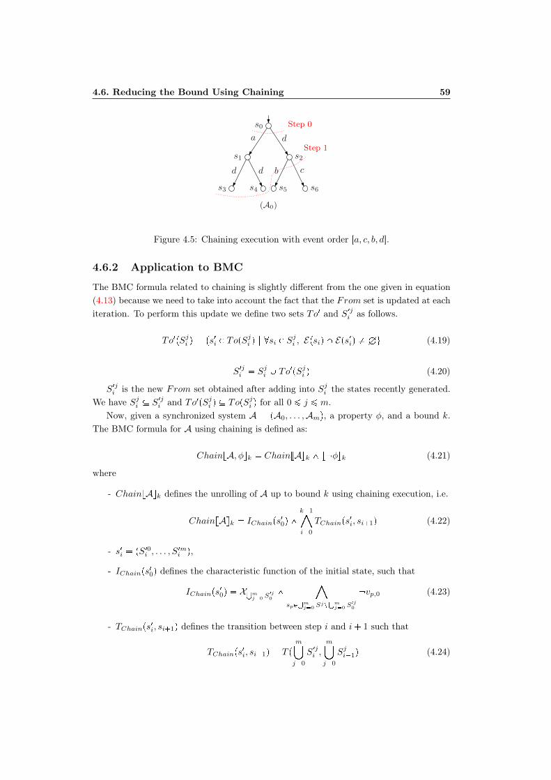
4.6. Reducing the Bound Using Chaining 59
Step 0
Step 1
s0
s1 s2
s3 s4 s5 s6
(A0)
a
d bd
d
c
Figure 4.5: Chaining execution with event order [a, c, b, d].
4.6.2 Application to BMC
The BMC formula related to chaining is slightly different from the one given in equation(4.13) because we need to take into account the fact that the From set is updated at eachiteration. To perform this update we define two sets To1 and S1ji as follows.
To1pSji q ts1i P TopS
ji q | @si P S
ji , Epsiq X Eps1iq Hu (4.19)
S1ji Sji Y To1pSji q (4.20)
S1ji is the new From set obtained after adding into Sji the states recently generated.We have Sji S1ji and To1pSji q TopSji q for all 0 ¤ j ¤ m.
Now, given a synchronized system A pA0, . . . ,Amq, a property φ, and a bound k.The BMC formula for A using chaining is defined as:
ChainvA, φwk ChainvAwk ^ v φwk (4.21)
where
- ChainvAwk defines the unrolling of A up to bound k using chaining execution, i.e.
ChainvAwk IChainps10q ^
k1©i0
TChainps1i, si1q (4.22)
- s1i pS10i , . . . , S1mi q,
- IChainps10q defines the characteristic function of the initial state, such that
IChainps10q Xm
j0 S1j0^
©spPm
j0 Sjzm
j0 S1j0
vp,0 (4.23)
- TChainps1i, si1q defines the transition between step i and i 1 such that
TChainps1i, si1q T p
m¤j0
S1ji ,m¤j0
Sji1q (4.24)
60 Encoding Methods
s0
s1 s2
s3 s4 s5 s6
(A0)
a
d bd
d
c
Step 0
Step 1
s7
s8
s9
(A1)
a
b
c
Figure 4.6: Chaining execution for synchronized systems.
Obviously, when applying chaining for synchronized products of TSs, we also have torespect the synchronization criteria described in Definition 4.4.2. This means, chainingcan be performed if the chosen event is either a local event, or it is enabled in all itscomponents at the current step.
Example 4.6.2 If we apply the chaining operation described in Figure 4.5 to thesynchronized systems A pA0,A1q in Figure 4.4, we obtain the following BMC formulaChainvAw1 for bound k 1 (the execution is depicted in Figure 4.6):
ChainvAw1 IChainppS100 , S
110 qq
^TChainppS100 , S
111 q, pS
01 , S
11qq
v0,0 ^ v1,0 ^ v7,0 ^ v2,0 ^ v3,0 ^ v4,0 ^ v5,0 ^ v6,0 ^ v8,0 ^ v9,0
^v0,0 ^ v1,0 ^ v7,0 ^ v0,1 ^ v1,1 ^ v7,1 ^ v2,1 ^ v3,1 ^ v4,1 ^ v8,1
^pv5,0 Ø v5,1q ^ pv6,0 Ø v6,1q ^ pv9,0 Ø v9,1q
where,
S00 ts0u; S
100 ts0, s1u; S
10 ts7u; S
110 ts7u; S
01 ts2, s3, s4u; S
11 ts8u;
E0 ta, du
We then have the following chaining execution:
pS100 , S110 q
E0ÝÑ pS01 , S
11q
Comparing the formula above with the one in Example 4.4.4 for k 2, we can seethat the equations for the transitions which lead to the states s3 and s4 can already beexpressed at bound 1. Therefore, a counterexample that exists in those states can befound at bound 1 instead of bound 2, if we choose the right order of events. In addition,the formula we obtain in here is clearly smaller than the one in Example 4.4.4.
Theorem 4.6.1Given a synchronized system A pA0, . . . ,Amq, a property φ, and a bound k. IfChainvA, φw is satisfiable then A * φ.
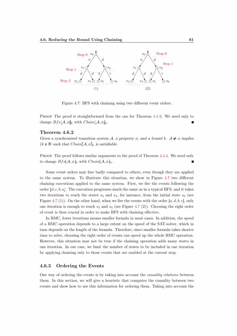
4.6. Reducing the Bound Using Chaining 61
Step 0
Step 1
Step 2
s0
s1 s2
s3 s4 s5 s6
p1q
a
d bd
d
c
Step 0
Step 1
s0
s1 s2
s3 s4 s5 s6
p2q
a
d bd
d
c
Figure 4.7: BFS with chaining using two different event orders.
Proof The proof is straightforward from the one for Theorem 4.4.3. We need only tochange BfsvA, φwk with ChainvA, φwk.
Theorem 4.6.2Given a synchronized transition system A, a property φ, and a bound k. A * φ impliesDk P N such that ChainvA, φwk is satisfiable.
Proof The proof follows similar arguments to the proof of Theorem 4.4.4. We need onlyto change BfsvA, φwk with ChainvA, φwk.
Some event orders may fare badly compared to others, even though they are appliedto the same system. To illustrate this situation, we show in Figure 4.7 two differentchaining executions applied to the same system. First, we fire the events following theorder rd, c, b, as. The execution progresses much the same as in a typical BFS, and it takestwo iterations to reach the states s3 and s4, for instance, from the initial state s0 (seeFigure 4.7 (1)). On the other hand, when we fire the events with the order ra, d, b, cs, onlyone iteration is enough to reach s3 and s4 (see Figure 4.7 (2)). Choosing the right orderof event is then crucial in order to make BFS with chaining effective.
In BMC, fewer iterations means smaller formula in most cases. In addition, the speedof a BMC operation depends to a large extent on the speed of the SAT-solver, which inturn depends on the length of the formula. Therefore, since smaller formula takes shortertime to solve, choosing the right order of events can speed up the whole BMC operation.However, this situation may not be true if the chaining operation adds many states inone iteration. In our case, we limit the number of states to be included in one iterationby applying chaining only to those events that are enabled at the current step.
4.6.3 Ordering the Events
One way of ordering the events is by taking into account the causality relations betweenthem. In this section, we will give a heuristic that computes the causality between twoevents and show how to use this information for ordering them. Taking into account the
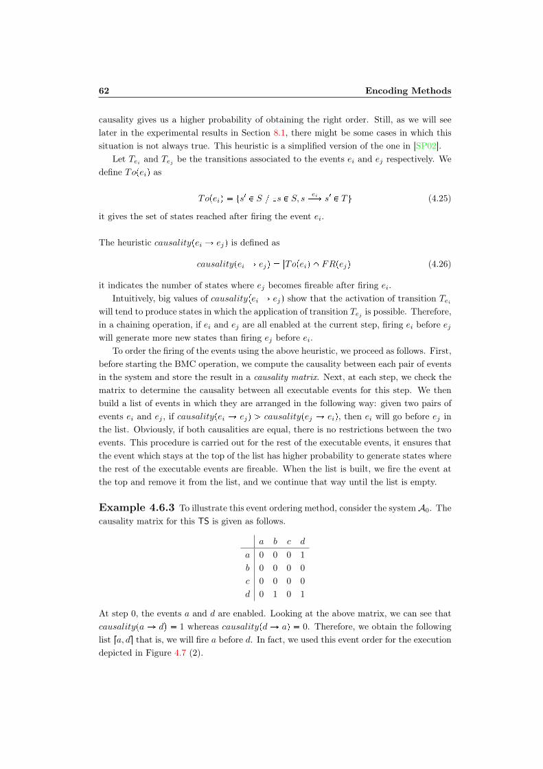
62 Encoding Methods
causality gives us a higher probability of obtaining the right order. Still, as we will seelater in the experimental results in Section 8.1, there might be some cases in which thissituation is not always true. This heuristic is a simplified version of the one in [SP02].
Let Tei and Tej be the transitions associated to the events ei and ej respectively. Wedefine Topeiq as
Topeiq ts1 P S Ds P S, s
eiÝÑ s1 P T u (4.25)
it gives the set of states reached after firing the event ei.
The heuristic causalitypei Ñ ejq is defined as
causalitypei Ñ ejq |Topeiq X FRpejq| (4.26)
it indicates the number of states where ej becomes fireable after firing ei.Intuitively, big values of causalitypei Ñ ejq show that the activation of transition Tei
will tend to produce states in which the application of transition Tej is possible. Therefore,in a chaining operation, if ei and ej are all enabled at the current step, firing ei before ejwill generate more new states than firing ej before ei.
To order the firing of the events using the above heuristic, we proceed as follows. First,before starting the BMC operation, we compute the causality between each pair of eventsin the system and store the result in a causality matrix. Next, at each step, we check thematrix to determine the causality between all executable events for this step. We thenbuild a list of events in which they are arranged in the following way: given two pairs ofevents ei and ej , if causalitypei Ñ ejq ¡ causalitypej Ñ eiq, then ei will go before ej inthe list. Obviously, if both causalities are equal, there is no restrictions between the twoevents. This procedure is carried out for the rest of the executable events, it ensures thatthe event which stays at the top of the list has higher probability to generate states wherethe rest of the executable events are fireable. When the list is built, we fire the event atthe top and remove it from the list, and we continue that way until the list is empty.
Example 4.6.3 To illustrate this event ordering method, consider the systemA0. Thecausality matrix for this TS is given as follows.
a b c d
a 0 0 0 1
b 0 0 0 0
c 0 0 0 0
d 0 1 0 1
At step 0, the events a and d are enabled. Looking at the above matrix, we can see thatcausalitypa Ñ dq 1 whereas causalitypd Ñ aq 0. Therefore, we obtain the followinglist ra, ds that is, we will fire a before d. In fact, we used this event order for the executiondepicted in Figure 4.7 (2).

4.6. Reducing the Bound Using Chaining 63
4.6.4 Chaining Algorithm
Algorithm 4.1 shows the BMC procedure related to chaining. computeFireableEvents()creates a list of fireable events an orders them using the heuristic above. The functionselectEvent() chooses an event from the list. chainFire() fires the chosen event, takinginto account all conditions described in this section, and building the BMC formula F inthe process. The function solve() calls the SAT-solver. It returns true if F is satisfiable,false otherwise. The algorithm stops whether the iteration reaches the maximum BMClength maxL or F is satisfiable.
Algorithm 4.1: Bmcinput : A pA0 . . .Anq synchronized TSs
maxL maximum BMC lengthoutput: true if a counterexample has been found
false otherwise
boundÐÝ 1 ;1
isSatÐÝ false ;2
while (bound ¤ maxL) and (isSat false) do3
for Aj P A do4
listÐÝ computeFireableEvents(Aj) ;5
while list H do6
eÐÝ selectEvent(list) ;7
F ÐÝ chainFire(e) ;8
end9
end10
isSatÐÝ solve(F) ;11
bound ;12
end13
return isSat14
Remark 4.6.1 Note that, to check a deadlock property with chaining we will also usethe formulas in equations (4.17) and (4.18).


Chapter 5
Leap-Based Approach
In this Chapter, we will present a method for increasing the speed of a BMC operation.Normally, in a typical BMC algorithm (see Algorithm 1.2), we call a SAT solver at eachexecution step. However, due to the possible huge number of steps needed for exploringconcurrent systems, we may need to perform many calls to a SAT solver during thewhole BMC operation. In addition, since solving SAT instances occupies a great deal oftime during the BMC operation, calling a solver too often will probably slow down theexecution, especially when dealing with sizeable formulas at a time.
One obvious way to cope with this problem is to use a fast SAT solver. But this solutionis helpful only for Boolean formulas with small sizes. For most of today’s solvers, theproblem still remains when they are called repeatedly to solve large formulas. The solutionwe propose consists in reducing the number of solver calls during a BMC operation,especially when the formulas become large. In this way, the speed will increase becausethe solver has to solve only few SAT instances.
Basically, our technique is performed as follows. When we move from one bound toanother, we do not carry out a simple one by one incrementation as in a standard BMCalgorithm. Instead, we use leaps. That is, we combine several unrolling steps together in asingle iteration before calling a SAT solver. One single bound in our method is, therefore,equivalent to several consecutive steps in a standard BMC algorithm.
The leap-based technique also applies to reachability properties. In order for it towork properly, it is important to ensure that we can catch all failure states occurringbetween BMC bounds even though we do not run a solver at the exact points where thesefailures occur. Otherwise, we would miss some counterexamples along the execution. Theunrolling methods we propose in this Chapter can handle this situation. They generate ateach bound a BMC formula that contains all necessary information needed for identifyingfailure states from earlier steps.
Figure 5.1 depicts the different steps for a leap execution. We have two types ofiterators, namely i and j, related to the BMC bounds and the steps needed betweenbounds respectively. All states sj correspond to the ones reached during the unrolling
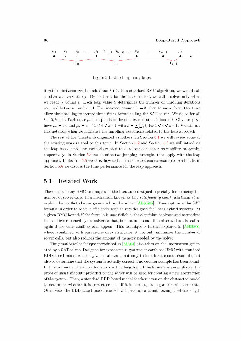
66 Leap-Based Approach
µ0 µ1 µ2 µk1 µks1 s2 sl01 sl02. . . . . . . . .
l0 l1 lk1
Figure 5.1: Unrolling using leaps.
iterations between two bounds i and i 1. In a standard BMC algorithm, we would calla solver at every step j. By contrast, for the leap method, we call a solver only whenwe reach a bound i. Each leap value li determines the number of unrolling iterationsrequired between i and i 1. For instance, assume l0 3, then to move from 0 to 1, weallow the unrolling to iterate three times before calling the SAT solver. We do so for alli P r0, k1s. Each state µ corresponds to the one reached at each bound i. Obviously, wehave µ0 s0, and µi sn @ 1 ¤ i ¤ k1 with n
°i1j1 lj for 1 ¤ i ¤ k1. We will use
this notation when we formalize the unrolling executions related to the leap approach.The rest of the Chapter is organized as follows. In Section 5.1 we will review some of
the existing work related to this topic. In Section 5.2 and Section 5.3 we will introducethe leap-based unrolling methods related to deadlock and other reachability propertiesrespectively. In Section 5.4 we describe two jumping strategies that apply with the leapapproach. In Section 5.5 we show how to find the shortest counterexample. An finally, inSection 5.6 we discuss the time performance for the leap approach.
5.1 Related Work
There exist many BMC techniques in the literature designed especially for reducing thenumber of solver calls. In a mechanism known as lazy satisfiability check, Ábráham et al.exploit the conflict clauses generated by the solver [ÁBKS05]. They optimize the SATformula in order to solve it efficiently with solvers designed for linear hybrid systems. Ata given BMC bound, if the formula is unsatisfiable, the algorithm analyzes and memorizesthe conflicts returned by the solver so that, in a future bound, the solver will not be calledagain if the same conflicts ever appear. This technique is further explored in [ÁHBS06]where, combined with parametric data structures, it not only minimizes the number ofsolver calls, but also reduces the amount of memory needed by the solver.
The proof-based technique introduced in [MA03] also relies on the information gener-ated by a SAT solver. Designed for synchronous systems, it combines BMC with standardBDD-based model checking, which allows it not only to look for a counterexample, butalso to determine that the system is actually correct if no counterexample has been found.In this technique, the algorithm starts with a length k. If the formula is unsatisfiable, theproof of unsatisfiability provided by the solver will be used for creating a new abstractionof the system. Then, a standard BDD-based model checker is ran on the abstracted modelto determine whether it is correct or not. If it is correct, the algorithm will terminate.Otherwise, the BDD-based model checker will produce a counterexample whose length
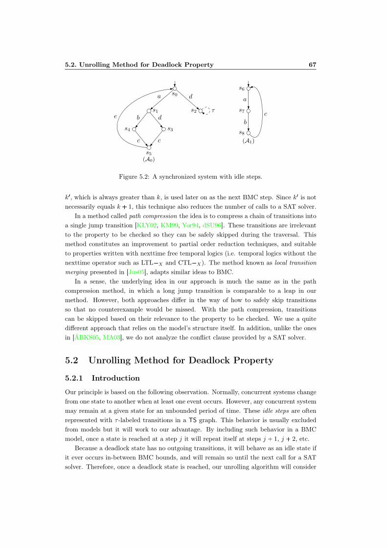
5.2. Unrolling Method for Deadlock Property 67
s0
s1 s2
s3s4
s5(A0)
a d
d
cc
beτ
s6
s7
s8
(A1)
a
b
c
Figure 5.2: A synchronized system with idle steps.
k1, which is always greater than k, is used later on as the next BMC step. Since k1 is notnecessarily equals k 1, this technique also reduces the number of calls to a SAT solver.
In a method called path compression the idea is to compress a chain of transitions intoa single jump transition [KLY02, KM99, Yor94, dSU96]. These transitions are irrelevantto the property to be checked so they can be safely skipped during the traversal. Thismethod constitutes an improvement to partial order reduction techniques, and suitableto properties written with nexttime free temporal logics (i.e. temporal logics without thenexttime operator such as LTLX and CTLX). The method known as local transitionmerging presented in [Jus05], adapts similar ideas to BMC.
In a sense, the underlying idea in our approach is much the same as in the pathcompression method, in which a long jump transition is comparable to a leap in ourmethod. However, both approaches differ in the way of how to safely skip transitionsso that no counterexample would be missed. With the path compression, transitionscan be skipped based on their relevance to the property to be checked. We use a quitedifferent approach that relies on the model’s structure itself. In addition, unlike the onesin [ÁBKS05, MA03], we do not analyze the conflict clause provided by a SAT solver.
5.2 Unrolling Method for Deadlock Property
5.2.1 Introduction
Our principle is based on the following observation. Normally, concurrent systems changefrom one state to another when at least one event occurs. However, any concurrent systemmay remain at a given state for an unbounded period of time. These idle steps are oftenrepresented with τ -labeled transitions in a TS graph. This behavior is usually excludedfrom models but it will work to our advantage. By including such behavior in a BMCmodel, once a state is reached at a step j it will repeat itself at steps j 1, j 2, etc.
Because a deadlock state has no outgoing transitions, it will behave as an idle state ifit ever occurs in-between BMC bounds, and will remain so until the next call for a SATsolver. Therefore, once a deadlock state is reached, our unrolling algorithm will consider
68 Leap-Based Approach
it as an idle state, and will repeat it over the execution. As a results, the state will keepits characteristics, and even though we do not call the SAT solver at the exact step wherethe deadlock occurs, we would not miss it at the next solver call.
For instance, assume a deadlock appears at the state s2 in Figure 5.2. If idle steps werenot allowed, then s2 would only be reachable by traces of length 1: s0
bÝÑ s2, or length
5: s0aÝÑ s1
bÝÑ s4
dÝÑ s5
dÝÑ s0
bÝÑ s2, or length 9 etc. But if idle steps are allowed,
we can reach s2 with traces of any length above 1, e.g. s0bÝÑ s2
τÝÑ s2
τÝÑ s2 . . .. We
express formally this key observation in the next theorem.
Theorem 5.2.1Let vAwk be the SAT formula related to the unrolling of the model A up to the boundk. If the unrolling allows idle steps, then there is a satisfying assignment of vAwk iff thereis a reachable state in A, reachable through sequence of steps of length i ¤ k (once idlesteps have been removed).
Proof The proof of the theorem is straightforward as it is clear that given any validunrolling, if a step is allowed to be idle, then all possible executions of length k includeall possible executions of some smaller length. For instance, all valid executions of lengthk 1 can be obtained from the executions of length k by changing the last step by theidle step.
5.2.2 BMC Equations
Let us now give the BMC equations related to this deadlock checking method. As usual,we consider interleaving, BFS, and Chaining executions. The big difference between theseequations and the ones in Section 4.4 can be seen in the transitions used. Here, we needto take into account the fact that we repeat each deadlock state over and over, until thenext solver call. Note that, there is no change for the deadlock conditions. We will stilluse the equations (4.17) and (4.18).
Given a synchronized model A pA0, . . . ,Amq, a property φ, a bound k, and naturalnumbers li ¡ 1 with i P r0, k 1s. The BMC formulas for A related to deadlock checking,defined in terms of the leaps li, is given as follows.
Interleaving Execution
lIntvA, φwk lIntvAwk ^ v φwk (5.1)
where
lIntvAwk IIntps0q ^k1©i0
TIlipµi, µi1q (5.2)
TIl0pµ0, µ1q l01©j0
TlIntpsj , sj1q (5.3)
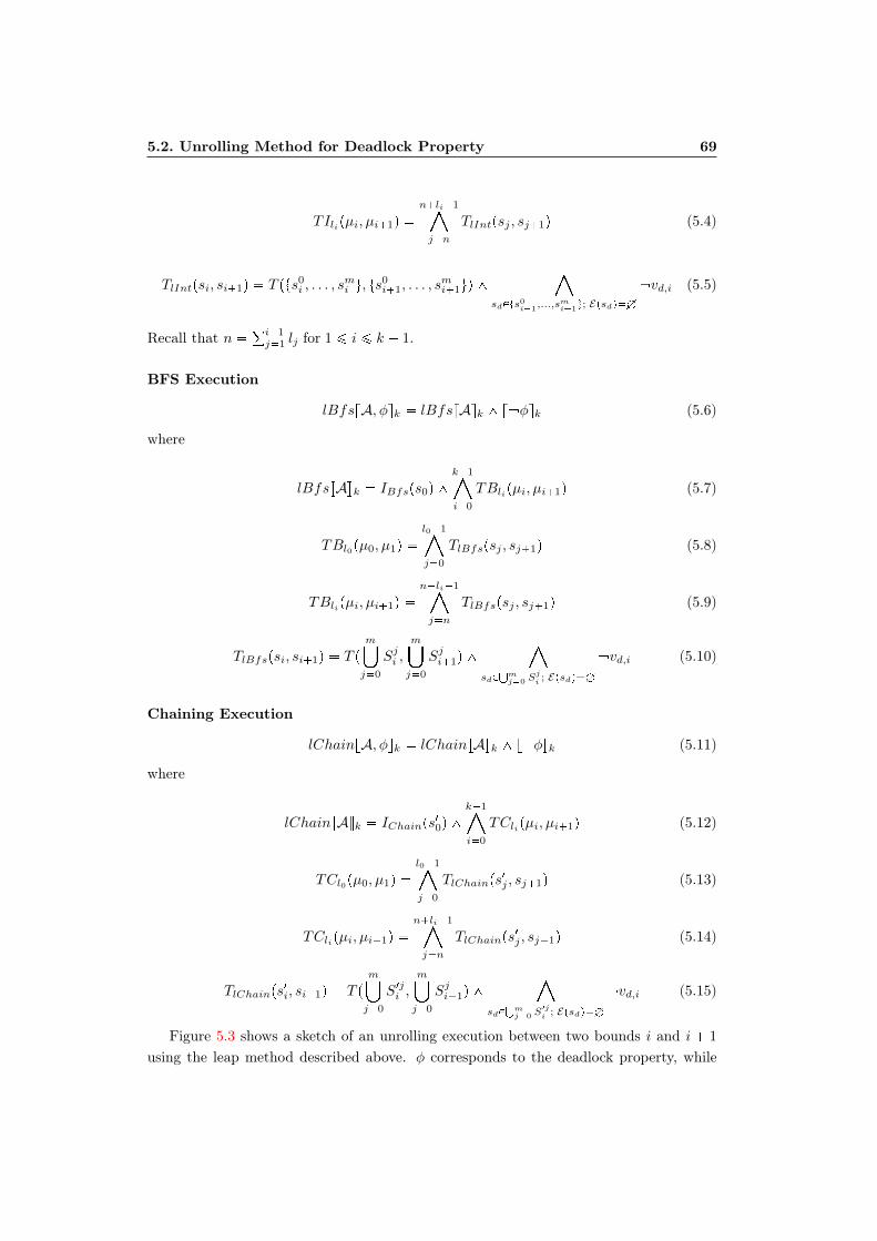
5.2. Unrolling Method for Deadlock Property 69
TIlipµi, µi1q nli1©jn
TlIntpsj , sj1q (5.4)
TlIntpsi, si1q T pts0i , . . . , s
mi u, ts
0i1, . . . , s
mi1uq ^
©sdPts0i1
,...,smi1u; EpsdqH
vd,i (5.5)
Recall that n °i1j1 lj for 1 ¤ i ¤ k 1.
BFS Execution
lBfsvA, φwk lBfsvAwk ^ v φwk (5.6)
where
lBfsvAwk IBfsps0q ^k1©i0
TBlipµi, µi1q (5.7)
TBl0pµ0, µ1q l01©j0
TlBfspsj , sj1q (5.8)
TBlipµi, µi1q nli1©jn
TlBfspsj , sj1q (5.9)
TlBfspsi, si1q T pm¤j0
Sji ,m¤j0
Sji1q ^©
sdPm
j0 Sji; EpsdqH
vd,i (5.10)
Chaining Execution
lChainvA, φwk lChainvAwk ^ v φwk (5.11)
where
lChainvAwk IChainps10q ^
k1©i0
TClipµi, µi1q (5.12)
TCl0pµ0, µ1q l01©j0
TlChainps1j , sj1q (5.13)
TClipµi, µi1q nli1©jn
TlChainps1j , sj1q (5.14)
TlChainps1i, si1q T p
m¤j0
S1ji ,m¤j0
Sji1q ^©
sdPm
j0 S1ji
; EpsdqH
vd,i (5.15)
Figure 5.3 shows a sketch of an unrolling execution between two bounds i and i 1
using the leap method described above. φ corresponds to the deadlock property, while
70 Leap-Based Approach
µi µi1sn1 sn2 sn3 . . .
SAT piq SAT pi 1q
v φwi v φwi1
Figure 5.3: Leap methods for deadlock property.
SAT piq indicates that we call the solver at bound i. We put the constraints related tothe negation of φ only at each bound i. Yet, by allowing idle steps, we could catch anycounterexample occurring at sn1, sn2, sn3, etc.
Example 5.2.1 Given the system depicted in Figure 5.2. As we can see, the states2 has no outgoing transitions. Therefore, the algorithm assumes there is an idle stepin this state, which is then repeated over and over until the next solver call. Using theBFS unrolling formulas from equations (5.6) and (5.9), we have the following formula fora leap execution between i 0 and i 1, with l0 3:
lBfsvAw1 v0,0 ^ v6,0 ^ v1,0 ^ v2,0 ^ v3,0 ^ v4,0 ^ v5,0 v7,0 v8,0
^v0,0 ^ v6,0 ^ v6,1 ^ v0,1 ^ v2,1 ^ v1,1 ^ v7,1 ^ pv3,0 Ø v3,1q
^pv4,0 Ø v4,1q ^ pv8,0 Ø v8,1q ^ pv5,0 Ø v5,1q
^v1,1 ^ v7,1 ^ v2,1 ^ v1,2 ^ v2,2 ^ v7,2 ^ v3,2 ^ v4,2 ^ v8,2
^pv0,1 Ø v0,2q ^ pv6,1 Ø v6,2q ^ pv5,1 Ø v5,2q
^v4,2 ^ v3,2 ^ v8,2 ^ v2,2 ^ v4,3 ^ v3,3 ^ v2,3 ^ v5,3 ^ v6,3
^pv1,2 Ø v1,3q ^ pv7,2 Ø v7,3q ^ pv0,2 Ø v0,3q
^ v1,3 ^ v2,3
5.3 Unrolling Method for Other Reachability Proper-ties
5.3.1 Introduction
In a BMC operation, the normal way is to add the constraints related to the negation of aproperty only when we call a SAT solver. This means that, in a leap-based unrolling, weshould put these constraints only at each bound i. As we have seen before, this approachworks perfectly for deadlock detection combined with idle step. But doing so with otherreachability properties would result in missed counterexamples because the informationrelated to these properties could not be maintained even though we repeat idle states overand over, so we would never know if any of the states in between BMC bounds violatesthe property to be checked. Therefore, to deal with other types of reachability properties,we need a different approach.
5.3. Unrolling Method for Other Reachability Properties 71
Our idea consists in putting the constraints related to the negation of the propertynot only at each bound i but also at each step j. In this way, even though we call thesolver at a later step we would not miss the counterexample. For sure, this method willincrease the size of the resulted formula, which would normally slows down the execution.However, we still can avoid this situation experimentally, by using the jumping methodsintroduced in Section 5.4. Figure 5.4 depicts an unrolling operation performed using thisapproach.
5.3.2 BMC Equations
Now, given a synchronized model A pA0, . . . ,Amq, a property φ, a bound k, and naturalnumbers li ¡ 1 with i P r0, k1s. The BMC formulas for A reachability checking, definedin terms of the leaps li, is given as follows.
Interleaving Execution
RlIntvAwk IIntps0q ^k1©i0
RIlipµi, µi1q (5.16)
where
RIl0pµ0, µ1q l01©j0
TIntpsj , sj1q ^ v φwj1 (5.17)
RIlipµi, µi1q nli1©jn
TIntpsj , sj1q ^ v φwj1 (5.18)
TIntpsi, si1q has been given in equation (4.12), and as usual, we have n °i1j1 lj for 1 ¤
i ¤ k 1.
BFS Execution
RlBfsvAwk IBfsps0q ^k1©i0
RBlipµi, µi1q (5.19)
where
RBl0pµ0, µ1q l01©j0
TBfspsj , sj1q ^ v φwj1 (5.20)
RBlipµi, µi1q nli1©jn
TBfspsj , sj1q ^ v φwj1 (5.21)
The relation TBfspsj , sj1q has been given in equation (4.16).

72 Leap-Based Approach
µi µi1sn1 sn2 sn3 . . .
SAT piq SAT pi 1q
v φwi v φwi1v φwn1 v φwn2 v φwn3
Figure 5.4: Leap methods for other reachability properties.
Chaining Execution
RlChainvAwk IChainps10q ^
k1©i0
RClipµi, µi1q (5.22)
where
RCl0pµ0, µ1q l01©j0
TChainps1j , sj1q ^ v φwj1 (5.23)
RClipµi, µi1q nli1©jn
TChainps1j , sj1q ^ v φwj1 (5.24)
The relation TChainps1j , sj1q has been given in equation (4.24).
Example 5.3.1 Consider again the system depicted in Figure 5.2. As we are nolonger verifying deadlock properties, idle steps do not apply anymore. Therefore, we putthe constraints related to the property at each step j. Using the BFS unrolling fromequations (5.19), (5.20), and (5.21), we have the following formula for a leap executionbetween i 0 and i 1, with l0 3:
leapvA, φw1 v0,0 ^ v1,0 ^ v2,0 ^ v3,0 ^ v4,0 ^ v5,0
^v0,0 ^ v0,1 ^ v1,1 ^ v2,1 ^ pv3,0 Ø v3,1q ^ pv4,0 Ø v4,1q
^pv5,0 Ø v5,1q^ v φw1
^v1,1 ^ v2,1 ^ v1,2 ^ v3,2 ^ v4,2 ^ v2,2 ^ pv0,1 Ø v0,2q
^pv5,1 Ø v5,2q^ v φw2
^v4,2 ^ v3,2 ^ v2,2 ^ v4,3 ^ v3,3 ^ v2,3 ^ v5,3 ^ pv1,2 Ø v1,3q
^pv0,2 Ø v0,3q^ v φw3
Obviously, each v φwj should be replaced with the formula related to the property tobe checked.
Remark 5.3.1 Although, we express all the equations in terms of synchronized tran-sition systems, we will see in Chapter 8 that the leap approach can also be applied toother types of models such as Petri net.
5.4. Jumping Methods 73
5.4 Jumping Methods
The efficiency of the leap approach depends to a large extent on the value of a leap li.Obviously, a big value of li indicates that the unrolling operation performs a long jumpat bound i. Similarly, a small value means a short jump. It is therefore, crucial to choosethe right value of each li. We will present in this section two heuristic algorithms usedfor choosing resoanable leap values.
5.4.1 Using Logarithmic Functions
As explained in Section 1.1.2, the size of the BMC formula is relatively small at an earlierstage of the execution and, consequently, the solver will run fast during this period. It is,therefore, beneficial to perform bigger jumps at the beginning in order to avoid calling aSAT solver frequently just for solving a small formula at a time.
Based on the above observation, we want the leaps to be bigger when the BMC exe-cution starts, and we want them to become smaller at upper bounds. When we increasethe bound, the formula grows in size as well, hence the solver will need more time andresources for solving it. Therefore, by performing short jumps at upper bounds, we canensure that the BMC formula will not be too big to handle by the solver.
The growth of base 2 logarithmic function log2pq, depicted in Figure 5.6, matchesexactly our above-mentioned scenario. If we construct a graph showing the executiontime of a BMC session, by associating the x axis to the CPU time spent at each bound,and the y axis to the bound value, we will obtain a graph similar to Figure 5.6. For thatreason, we choose the log2pq function as a way of determining the leaps.
We determine the leap in the following way. We set up various CPU time thresholds,each of them corresponds to the one consumed by a SAT solver at each execution step.When the value is really small, i.e. below a given minimum threshold, or when it is toobig, i.e. beyond a given maximum threshold, we use a small constant leap. We also setup another middle value between the minimum and maximum time interval. In order togo deep faster, we multiply the logarithmic function with the small constant leap beforewe reach the middle value.
When the maximum value is reached, we use only the small constant in order to havesmaller leaps up to a certain huge CPU time limit. This limit is reached when the formulabecomes too big to be solved by a SAT solver. In this case, we backtrack to the previousstep, recompute the leap by dividing the latest one by two, and rejump accordingly.
Using the above method allows us always to obtain a BMC formula manageable bythe solver even though we put several steps together in a single SAT check.
These different leap values are depicted in Figure 5.5, where k is the constant leap,log2 is the base 2 logarithmic function, and b is the bound.
Note that in this jumping strategy we assume the BMC execution to follow the generalcase, that is, the deeper you go, the slower the execution. However, in certain situations,the solver may run faster at a very deep depth value.
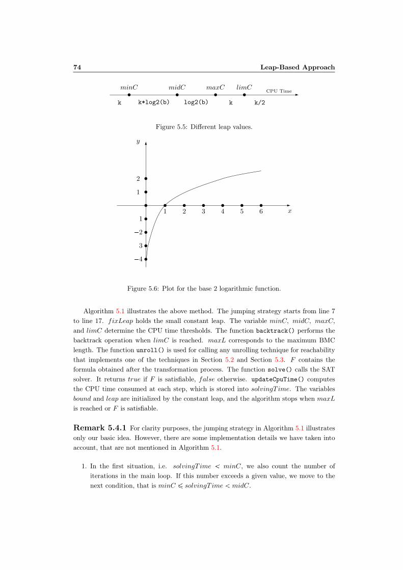
74 Leap-Based Approach
minC midC maxC limCCPU Time
k k*log2(b) log2(b) k k/2
Figure 5.5: Different leap values.
1 2 3 4 5 6 x
y
1
2
1
2
3
4
Figure 5.6: Plot for the base 2 logarithmic function.
Algorithm 5.1 illustrates the above method. The jumping strategy starts from line 7to line 17. fixLeap holds the small constant leap. The variable minC, midC, maxC,and limC determine the CPU time thresholds. The function backtrack() performs thebacktrack operation when limC is reached. maxL corresponds to the maximum BMClength. The function unroll() is used for calling any unrolling technique for reachabilitythat implements one of the techniques in Section 5.2 and Section 5.3. F contains theformula obtained after the transformation process. The function solve() calls the SATsolver. It returns true if F is satisfiable, false otherwise. updateCpuTime() computesthe CPU time consumed at each step, which is stored into solvingT ime. The variablesbound and leap are initialized by the constant leap, and the algorithm stops when maxLis reached or F is satisfiable.
Remark 5.4.1 For clarity purposes, the jumping strategy in Algorithm 5.1 illustratesonly our basic idea. However, there are some implementation details we have taken intoaccount, that are not mentioned in Algorithm 5.1.
1. In the first situation, i.e. solvingT ime minC, we also count the number ofiterations in the main loop. If this number exceeds a given value, we move to thenext condition, that is minC ¤ solvingT ime midC.

5.4. Jumping Methods 75
Algorithm 5.1: JumpByLogarithminput : P a 1-safe Petri net
maxL maximum BMC lengthminC,midC,maxC, limC time thresholdsfixLeap fixed constant leapidleMethod unrolling method with idle step
output: true if a counterexample has been foundfalse otherwise
boundÐÝ fixLeap ;1
isSatÐÝ false ;2
while (bound ¤ maxL) and (isSat false) do3
F ÐÝ unroll(P, bound, idleMethod) ;4
isSatÐÝ solve(F) ;5
solvingT imeÐÝ updateCpuTime () ;6
if solvingT ime minC then7
leapÐÝ fixLeap ;8
else if minC ¤ solvingT ime midC then9
leapÐÝ fixLeap log2(bound) ;10
else if midC ¤ solvingT ime maxC then11
leapÐÝ log2(bound) ;12
else if maxC ¤ solvingT ime limC then13
leapÐÝ fixLeap ;14
else if solvingT ime ¤ limC then15
leapÐÝ leap 2 ;16
backtrack(bound) ;17
boundÐÝ bound leap ;18
end19
return isSat20
2. We restrict the fixLeap value to be a very small integer, but greater than 1. Inthis way, we could avoid the problem discussed at the beginning of this Chapterrelated to the speed of the whole leap operation. So far the values we used for ourbenchmarks are around 4, i.e. 3, 4, or 5.
3. When limC is reached, we also count the number of backtrack operations, and thealgorithm stops when it comes back to the latest bound the solver was able to check.In addition, dividing the leap by 2 may yields a value equals 1. In this case, thealgorithm stops.
4 For the the CPU time thresholds minC, midC, maxC, and limC, there are nostandard values that work for all benchmarks. These constants are chosen while

76 Leap-Based Approach
performing the experimentations. In addition, some of those constants may not beused at all. For instance, if the formula is satisfiable between midC and maxC,then we will not reach the constant maxC and limC. The important thing hereis to understand the idea behind the method, but one should performs a couple oftests in order to know which values work best for each benchmark.
5.4.2 Using Interpolation
In this heuristic we use interpolation-extrapolation methods instead of the base 2 loga-rithmic function as explained below.
In many cases, SAT solving times steadily increase throughout the BMC executionuntil we reach a point where the circuit becomes satisfiable. Therefore, we want toestimate, for each benchmark, the bound at which the CPU time limit could be reached.We also prefer not to spend too much time in smaller bounds and try to use the availableresources to go as deep as possible. All this can be achieved by jumping directly to theestimated bound just after a few execution steps.
To perform the estimation, a number of data points containing the bounds and theCPU time spent for each bound have to be collected during the initial phase of a BMCexecution. A fix constant leap is used while collecting the data points, and the collectionprocess stops when a given CPU time is reached. A curve is then constructed out ofthese points, and extrapolated to reach the CPU time limit. However, for the extrap-olation function to work properly, these data points need to be smoothed. We use thesmoothing method introduced in [Rei67] and the well-known Newton polynomial for theextrapolation. When all these operations are finished, the algorithm jumps directly to theestimated bound obtained by the extrapolation function. However, the generated boundvalue is merely an estimation. That is, it doesn’t necessarily mean that the CPU timelimit is actually reached at this bound. But, in case this limit is really reached we do thesame procedure as in the previous jumping method. Figure 5.7 explains the interpolationmethod.
Algorithm 5.2: jumpByInterpolation
. . .1
dataÐÝ addPoint (bound, solvingT ime) ;2
if solvingT ime ¤ midC then3
leapÐÝ fixLeap ;4
else if midC solvingT ime limC then5
leapÐÝ interpolate (data) ;6
. . .7
Now, if we use this jumping scheme, the lines 7 to 14 in Algorithm 5.1 will be replacedby the lines 2 to 6 in Algorithm 5.2. Here, the points to be interpolated are stored inthe variable data. These points consist of the bounds with their corresponding solving
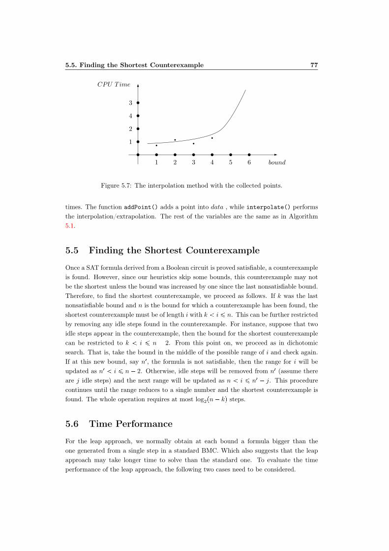
5.5. Finding the Shortest Counterexample 77
1 2 3 4 5 6 bound
CPU Time
4
3
2
1
Figure 5.7: The interpolation method with the collected points.
times. The function addPoint() adds a point into data , while interpolate() performsthe interpolation/extrapolation. The rest of the variables are the same as in Algorithm5.1.
5.5 Finding the Shortest Counterexample
Once a SAT formula derived from a Boolean circuit is proved satisfiable, a counterexampleis found. However, since our heuristics skip some bounds, this counterexample may notbe the shortest unless the bound was increased by one since the last nonsatisfiable bound.Therefore, to find the shortest counterexample, we proceed as follows. If k was the lastnonsatisfiable bound and n is the bound for which a counterexample has been found, theshortest counterexample must be of length i with k i ¤ n. This can be further restrictedby removing any idle steps found in the counterexample. For instance, suppose that twoidle steps appear in the counterexample, then the bound for the shortest counterexamplecan be restricted to k i ¤ n 2. From this point on, we proceed as in dichotomicsearch. That is, take the bound in the middle of the possible range of i and check again.If at this new bound, say n1, the formula is not satisfiable, then the range for i will beupdated as n1 i ¤ n 2. Otherwise, idle steps will be removed from n1 (assume thereare j idle steps) and the next range will be updated as n i ¤ n1 j. This procedurecontinues until the range reduces to a single number and the shortest counterexample isfound. The whole operation requires at most log2pn kq steps.
5.6 Time Performance
For the leap approach, we normally obtain at each bound a formula bigger than theone generated from a single step in a standard BMC. Which also suggests that the leapapproach may take longer time to solve than the standard one. To evaluate the timeperformance of the leap approach, the following two cases need to be considered.
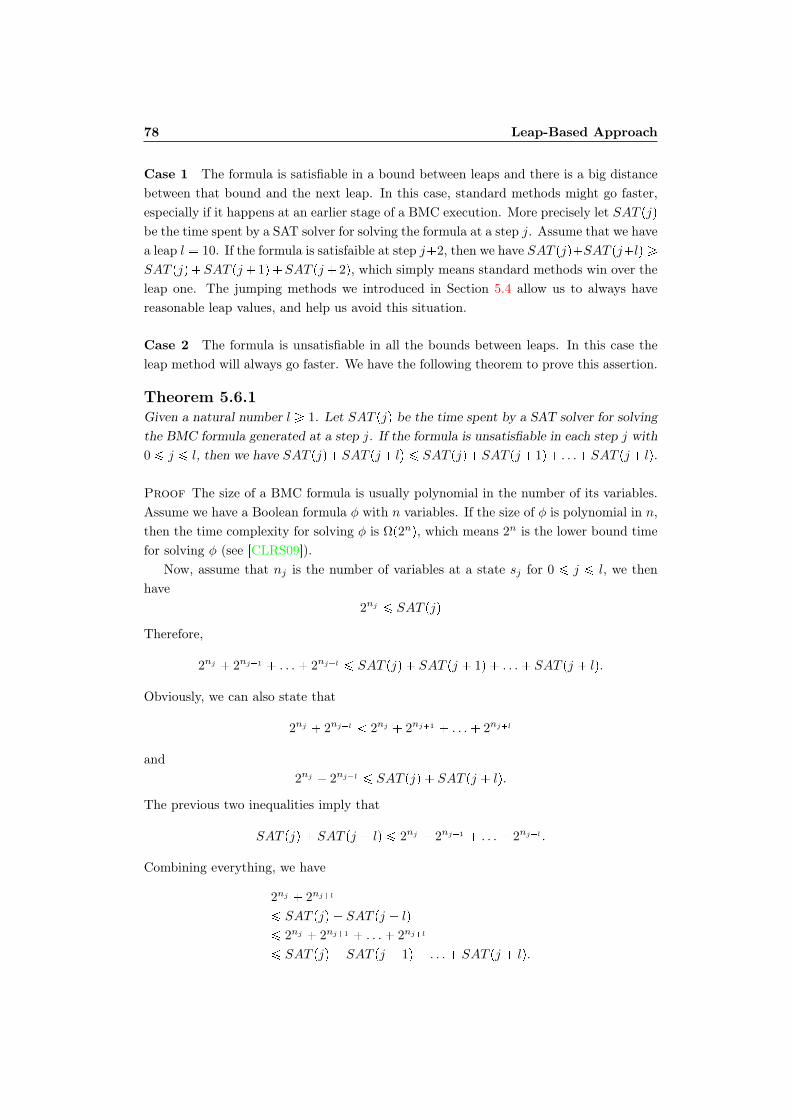
78 Leap-Based Approach
Case 1 The formula is satisfiable in a bound between leaps and there is a big distancebetween that bound and the next leap. In this case, standard methods might go faster,especially if it happens at an earlier stage of a BMC execution. More precisely let SAT pjqbe the time spent by a SAT solver for solving the formula at a step j. Assume that we havea leap l 10. If the formula is satisfaible at step j2, then we have SAT pjqSAT pjlq ¥SAT pjqSAT pj 1qSAT pj 2q, which simply means standard methods win over theleap one. The jumping methods we introduced in Section 5.4 allow us to always havereasonable leap values, and help us avoid this situation.
Case 2 The formula is unsatisfiable in all the bounds between leaps. In this case theleap method will always go faster. We have the following theorem to prove this assertion.
Theorem 5.6.1Given a natural number l ¥ 1. Let SAT pjq be the time spent by a SAT solver for solvingthe BMC formula generated at a step j. If the formula is unsatisfiable in each step j with0 ¤ j ¤ l, then we have SAT pjqSAT pj lq ¤ SAT pjqSAT pj1q . . .SAT pj lq.
Proof The size of a BMC formula is usually polynomial in the number of its variables.Assume we have a Boolean formula φ with n variables. If the size of φ is polynomial in n,then the time complexity for solving φ is Ωp2nq, which means 2n is the lower bound timefor solving φ (see [CLRS09]).
Now, assume that nj is the number of variables at a state sj for 0 ¤ j ¤ l, we thenhave
2nj ¤ SAT pjq
Therefore,
2nj 2nj1 . . . 2njl ¤ SAT pjq SAT pj 1q . . . SAT pj lq.
Obviously, we can also state that
2nj 2njl 2nj 2nj1 . . . 2njl
and2nj 2njl ¤ SAT pjq SAT pj lq.
The previous two inequalities imply that
SAT pjq SAT pj lq ¤ 2nj 2nj1 . . . 2njl .
Combining everything, we have
2nj 2njl
¤ SAT pjq SAT pj lq
¤ 2nj 2nj1 . . . 2njl
¤ SAT pjq SAT pj 1q . . . SAT pj lq.
5.6. Time Performance 79
We then conclude that
SAT pjq SAT pj lq ¤ SAT pjq SAT pj 1q . . . SAT pj lq
We should also mention that many of today’s BMC tools also include a switch toallow the user to specify a (fixed) increment size. Our heuristics may sound a littlecomplicated, but the advantage of using them is that, they allow the incrementationto be done automatically and not in fixed size, especially for the interpolation method.In addition, these methods can be very helpful when the user is first attacking a newproblem since it is not always evident to start directly with a fixed increment size unlessone knows what to expect from the system. Hence, using a method that allows automaticincrementing can be helpful in this situation. Moreover, the learning and incrementalmechanisms that exist in today’s SAT solver help to maintain the information from theprevious check. Thus, it helps as well to speed up the execution.

Chapter 6
An Automata-TheoreticApproach
Even though they are efficient, all the encodings discussed in Chapter 4 and Chapter 5apply only to reachability. In this chapter, we improve the methods in order to check othertypes of properties. Here, we adopt the logic LTL as a specification formalism since it canexpress a broad range of properties including safety, liveness, and fairness. Furthermore,it has a path-like structure well suited for a BMC operation.
To perform the unrolling, we do not construct a Boolean formula directly out of anLTL specification. Rather, we apply the technique known as automata-theoretic approach,in which the LTL formula is first translated into an automaton on infinite words, knownas Büchi automaton, before encoding it into a Boolean formula [VW86, WVS83]. Theobjective is to associate each LTL formula with a Büchi automaton that accepts exactlyall infinite words modeling the formula. This approach reduces the LTL model checkingproblem into known automata-theoretic problems. In this way, some existing automata-related algorithms can be used to solve the model checking problem. Translating the LTLformula into an automaton may appear to add extra cost to the model checking process,but it has been shown experimentally that for most of the LTL formulas regularly usedin formal verification, the resulting automata is often small [Wol02]. Consequently, thesize of the Boolean formula constructed from the automaton can be small as well, whichis really helpful especially for a BMC operation. Moreover, creating a Boolean formulafrom an automaton is often simpler than creating it directly from the LTL formula itself.
Automata-theoretic approaches are performed in the following way: build first theautomaton representing the state graph of the system, next translate the negation ofthe LTL formula into a Büchi automaton, then build a new automaton formed by thesynchronized product of the two, and finally conduct an emptiness check of the product,i.e. check if there is an infinite word accepted by the new automaton. If such a wordexists, it corresponds to a counterexample.
The above-mentioned steps are commonly used to deal with unbounded model check-

82 An Automata-Theoretic Approach
System A LTL formula φ
Buchi automaton for φ
Unrolling of the Buchi automaton
Unrolling of A
Conjunction of the unrollings
Solver
Result
Counterexample No counterexample
Figure 6.1: Automata-theoretic approach to BMC.
ing. Since our focus is on BMC, our technique is quite different, especially in the laststep. We do not build a new product automaton. Rather, we translate separately the twoautomata into Boolean formulas, and then construct the conjunction of the two formulas.The whole operation is divided in four principal tasks (see Figure 6.1):
1. build the unrolling of the system up to a bound k;
2. translate the negation of the LTL formula into a Büchi automaton;
3. build the unrolling of the automaton up to k;
4. compute the conjunction of the two unrollings.
We apply our technique to synchronized product of transition systems. The LTLspecifications we are checking concern the events of the system. Therefore, to performthe unrolling of the TSs, we extend the encodings introduced in Chapter 4 by includinginto the formulas some information concerning the enabled events.
We are mainly interested in the type of Büchi automata known as transition-basedgeneralized Büchi automata (TGBA). There are two main reasons for this choice. First,in theoretical viewpoint, the TS model and TGBA are graph-based formalisms that haveroughly the same structure. As a result, it is much simpler to build the conjunctionbetween the TS unrolling and the one constructed from the automata. Second, practically,
6.1. Related Work 83
it has been proven that translating LTL formulas into TGBA yields smaller automata (seee.g. [DLP04]).
The rest of the chapter is organized as follows. In Section 6.1, we review some workin the literature related to this topic. In Section 6.2, we will discuss the Büchi automataencodings. In Section 6.3, we will introduce the BMC encodings.
6.1 Related Work
Automata-theoretic approaches are much more common in unbounded model checking[DLP04, AEF05, She05, Var95, VW86, Var06]. Some people also apply it to on-the-flymodel checking, in which the principal steps consist in building on demand the automatonrelated to an LTL formula, and then performing an on-the-fly emptiness check on theproduct automaton [CVWY92, GH93, Hol88, CDLP05]. This approach can be combinedwith Tarjan’s algorithm as discussed in [JV04, GH93]. In [Cou99], Courveur proposedanother variant of this algorithm, which can perform fairness checking without needlessoverhead.
The most closely related to ours is the BMC approach introduced in [Sor02], whichalso generates the Boolean formula by constructing the conjunction of the two formulasobtained from the LTL transformation and the system model respectively. However,the big difference is that the method in [Sor02] applies to timed automata rather thantransition systems.
The BMC method in [dMRS02, CKOS04], by contrast, is performed by searching forfair loop counterexamples in the product system. Although the search can sometimesgo deeper than in other methods, it does not produce linear sized Boolean formulas.Combining this method with other encodings such as the ones in [CPRS02, LBHJ04]could possibly improve the results.
A method for translating an LTL formula into a symbolic Büchi automaton is alsointroduced in [CGH94]. The translation produces a result ready to be used for symbolicmodel checking, and it runs in time Op|φ|q, where φ is the LTL formula. Nevertheless,the number of states in the automaton may sometimes blow up exponentially. Shneidersuggested a way to go around this problem in [Sch99], while Schuppan et al. discussed apossible application of this method to BMC in [SB05].
Note Most early work on BMC with LTL is based on the encoding introduced by Biereet al. [BCCZ99], in which they translate LTL specifications directly into Boolean formulas.They also encode loop and nonloop executions differently, whereas subsequent techniquesuse the same encoding for both (e.g. [CPRS02, FSW02]).
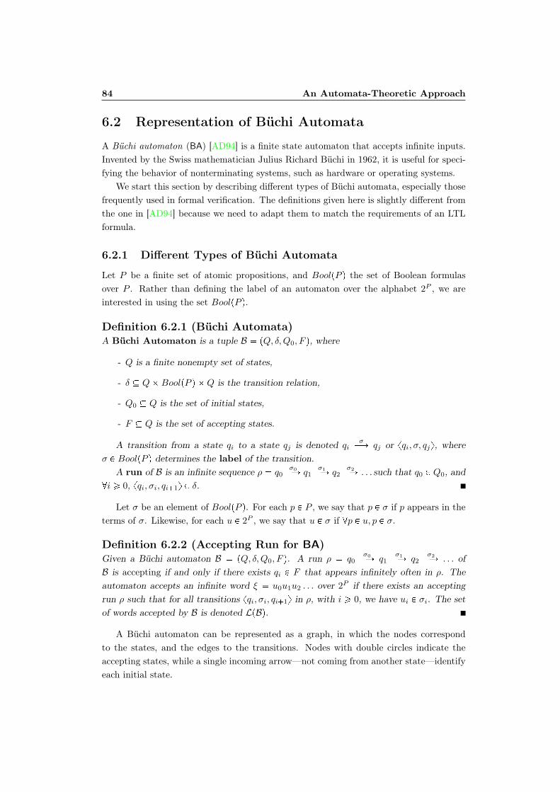
84 An Automata-Theoretic Approach
6.2 Representation of Büchi Automata
A Büchi automaton (BA) [AD94] is a finite state automaton that accepts infinite inputs.Invented by the Swiss mathematician Julius Richard Büchi in 1962, it is useful for speci-fying the behavior of nonterminating systems, such as hardware or operating systems.
We start this section by describing different types of Büchi automata, especially thosefrequently used in formal verification. The definitions given here is slightly different fromthe one in [AD94] because we need to adapt them to match the requirements of an LTLformula.
6.2.1 Different Types of Büchi Automata
Let P be a finite set of atomic propositions, and BoolpP q the set of Boolean formulasover P . Rather than defining the label of an automaton over the alphabet 2P , we areinterested in using the set BoolpP q.
Definition 6.2.1 (Büchi Automata)A Büchi Automaton is a tuple B pQ, δ,Q0, F q, where
- Q is a finite nonempty set of states,
- δ QBoolpP q Q is the transition relation,
- Q0 Q is the set of initial states,
- F Q is the set of accepting states.
A transition from a state qi to a state qj is denoted qiσÝÑ qj or xqi, σ, qjy, where
σ P BoolpP q determines the label of the transition.A run of B is an infinite sequence ρ q0
σ0ÝÑ q1σ1ÝÑ q2
σ2ÝÑ . . . such that q0 P Q0, and@i ¥ 0, xqi, σi, qi1y P δ.
Let σ be an element of BoolpP q. For each p P P , we say that p P σ if p appears in theterms of σ. Likewise, for each u P 2P , we say that u P σ if @p P u, p P σ.
Definition 6.2.2 (Accepting Run for BA)Given a Büchi automaton B pQ, δ,Q0, F q. A run ρ q0
σ0ÝÑ q1σ1ÝÑ q2
σ2ÝÑ . . . ofB is accepting if and only if there exists qi P F that appears infinitely often in ρ. Theautomaton accepts an infinite word ξ u0u1u2 . . . over 2P if there exists an acceptingrun ρ such that for all transitions xqi, σi, qi1y in ρ, with i ¥ 0, we have ui P σi. The setof words accepted by B is denoted LpBq.
A Büchi automaton can be represented as a graph, in which the nodes correspondto the states, and the edges to the transitions. Nodes with double circles indicate theaccepting states, while a single incoming arrow—not coming from another state—identifyeach initial state.
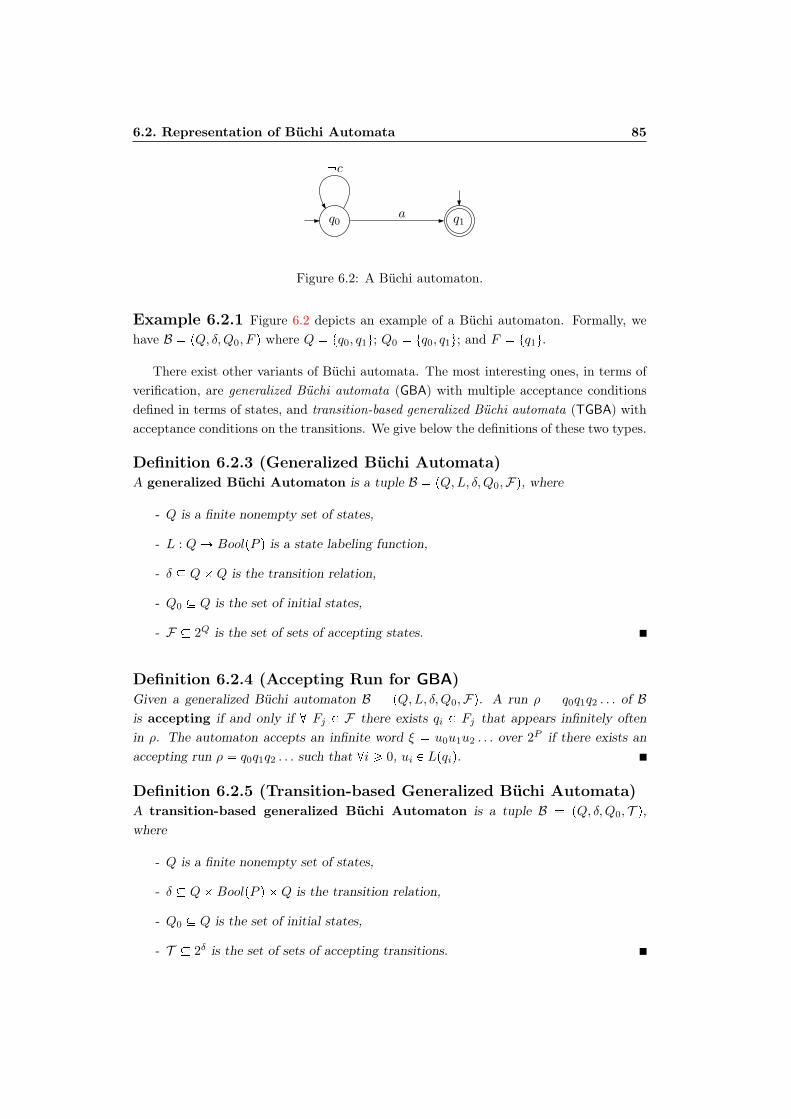
6.2. Representation of Büchi Automata 85
q0 q1
c
a
Figure 6.2: A Büchi automaton.
Example 6.2.1 Figure 6.2 depicts an example of a Büchi automaton. Formally, wehave B pQ, δ,Q0, F q where Q tq0, q1u; Q0 tq0, q1u; and F tq1u.
There exist other variants of Büchi automata. The most interesting ones, in terms ofverification, are generalized Büchi automata (GBA) with multiple acceptance conditionsdefined in terms of states, and transition-based generalized Büchi automata (TGBA) withacceptance conditions on the transitions. We give below the definitions of these two types.
Definition 6.2.3 (Generalized Büchi Automata)A generalized Büchi Automaton is a tuple B pQ,L, δ,Q0,Fq, where
- Q is a finite nonempty set of states,
- L : QÑ BoolpP q is a state labeling function,
- δ QQ is the transition relation,
- Q0 Q is the set of initial states,
- F 2Q is the set of sets of accepting states.
Definition 6.2.4 (Accepting Run for GBA)Given a generalized Büchi automaton B pQ,L, δ,Q0,Fq. A run ρ q0q1q2 . . . of Bis accepting if and only if @ Fj P F there exists qi P Fj that appears infinitely oftenin ρ. The automaton accepts an infinite word ξ u0u1u2 . . . over 2P if there exists anaccepting run ρ q0q1q2 . . . such that @i ¥ 0, ui P Lpqiq.
Definition 6.2.5 (Transition-based Generalized Büchi Automata)A transition-based generalized Büchi Automaton is a tuple B pQ, δ,Q0, T q,where
- Q is a finite nonempty set of states,
- δ QBoolpP q Q is the transition relation,
- Q0 Q is the set of initial states,
- T 2δ is the set of sets of accepting transitions.

86 An Automata-Theoretic Approach
q0 q1
c
a
Figure 6.3: A Transition-based Büchi automaton.
Definition 6.2.6 (Accepting Run for TGBA)Given a transition-based generalized Büchi automaton B pQ, δ,Q0, T q. A run ρ
q0σ0ÝÑ q1
σ1ÝÑ q2σ2ÝÑ . . . of B is accepting if and only if @ Tj P T there exists ti P Tj that
appears infinitely often in ρ. The automaton accepts an infinite word ξ u0u1u2 . . . over2P if there exists an accepting run ρ such that for all transitions xqi, σi, qi1y in ρ, withi ¥ 0, we have ui P σi.
Lemma 6.2.1Given a generalized Büchi automaton, one can build an equivalent transition-based gen-eralized Büchi automaton, and vice versa.
Proof (ñ) All we need to do is move the labels and the acceptance conditions fromstates to transitions. An accepting transition in a TGBA is simply one that leads to anaccepting state in the corresponding GBA. Therefore, assume that we have a GBA with anaccepting set F tF1, F2, . . . , Fnu, we can build a TGBA with an accepting set T , suchthat |T | |F |, and the elements of a set Ti P T correspond to all incoming transitionsof the states in Fi. i.e. for all t qa
σÝÑ qb P Ti in the TGBA, we have qb P Fi in the
corresponding GBA.(ð) Follows by similar argumentation.
Example 6.2.2 Figure 6.3 depicts a TGBA version of the automaton in Example 6.2.1.Accepting transitions are represented as dashed lines. Formally, we have B pQ, δ,Q0, T qwhere, Q tq0, q1u; Q0 tq0, q1u; and T ttq0
aÝÑ q1uu.
6.2.2 Translating an LTL Formula Into a TGBA
Translating an LTL formula into a Büchi automata is a whole independent topic thathas already been investigated thoroughly by many researchers (see e.g. [DGV99, SB00,DLP04, Tau03, EH00, GO01]). In our work, we use the technique introduced in [GPVW95].With this translation, the labels and acceptance conditions are defined in terms of statesrather than transition. Therefore, to obtain a TGBA, we simply push the labels into thetransitions after the translation, and adjust the acceptance conditions accordingly.
The translation is performed using the tableau rules shown in Table 6.1. The rulesare applied to a formula φ until it becomes an expression composed only of elementary
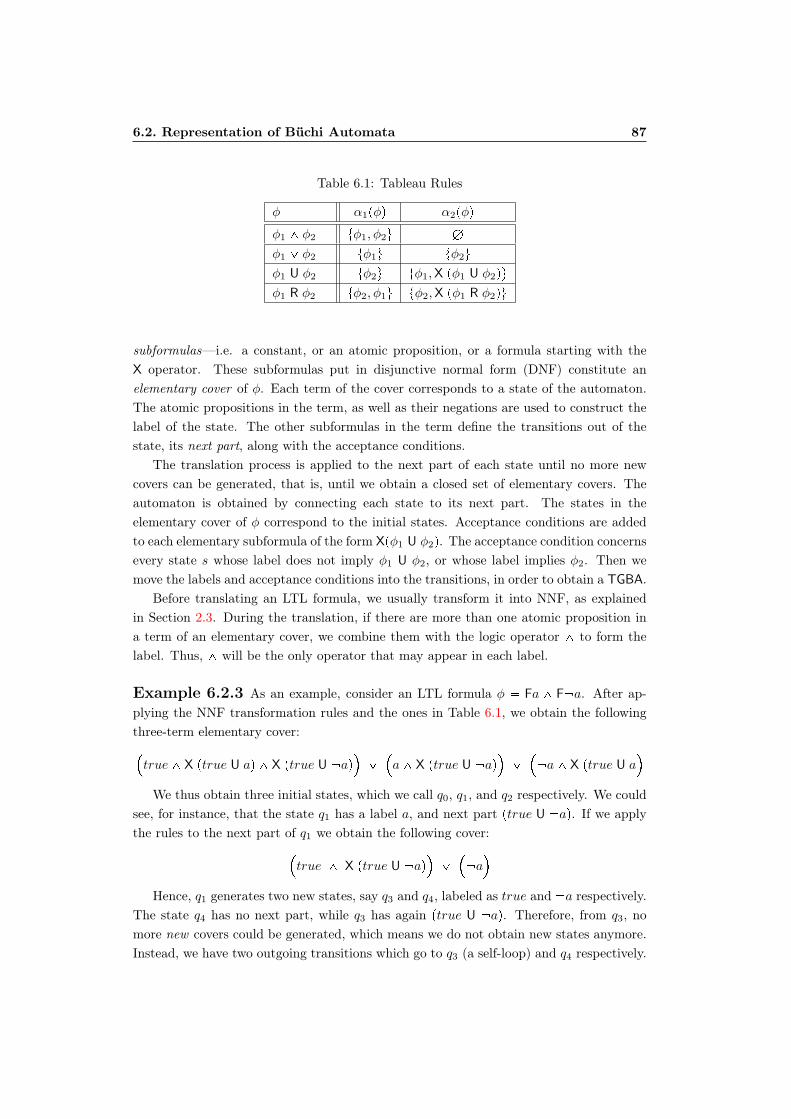
6.2. Representation of Büchi Automata 87
Table 6.1: Tableau Rules
φ α1pφq α2pφq
φ1 ^ φ2 tφ1, φ2u H
φ1 _ φ2 tφ1u tφ2u
φ1 U φ2 tφ2u tφ1,X pφ1 U φ2qu
φ1 R φ2 tφ2, φ1u tφ2,X pφ1 R φ2qu
subformulas—i.e. a constant, or an atomic proposition, or a formula starting with theX operator. These subformulas put in disjunctive normal form (DNF) constitute anelementary cover of φ. Each term of the cover corresponds to a state of the automaton.The atomic propositions in the term, as well as their negations are used to construct thelabel of the state. The other subformulas in the term define the transitions out of thestate, its next part, along with the acceptance conditions.
The translation process is applied to the next part of each state until no more newcovers can be generated, that is, until we obtain a closed set of elementary covers. Theautomaton is obtained by connecting each state to its next part. The states in theelementary cover of φ correspond to the initial states. Acceptance conditions are addedto each elementary subformula of the form Xpφ1 U φ2q. The acceptance condition concernsevery state s whose label does not imply φ1 U φ2, or whose label implies φ2. Then wemove the labels and acceptance conditions into the transitions, in order to obtain a TGBA.
Before translating an LTL formula, we usually transform it into NNF, as explainedin Section 2.3. During the translation, if there are more than one atomic proposition ina term of an elementary cover, we combine them with the logic operator ^ to form thelabel. Thus, ^ will be the only operator that may appear in each label.
Example 6.2.3 As an example, consider an LTL formula φ Fa ^ F a. After ap-plying the NNF transformation rules and the ones in Table 6.1, we obtain the followingthree-term elementary cover:true^ X ptrue U aq ^ X ptrue U aq
_a^ X ptrue U aq
_ a^ X ptrue U a
We thus obtain three initial states, which we call q0, q1, and q2 respectively. We couldsee, for instance, that the state q1 has a label a, and next part ptrue U aq. If we applythe rules to the next part of q1 we obtain the following cover:
true ^ X ptrue U aq
_ a
Hence, q1 generates two new states, say q3 and q4, labeled as true and a respectively.The state q4 has no next part, while q3 has again ptrue U aq. Therefore, from q3, nomore new covers could be generated, which means we do not obtain new states anymore.Instead, we have two outgoing transitions which go to q3 (a self-loop) and q4 respectively.
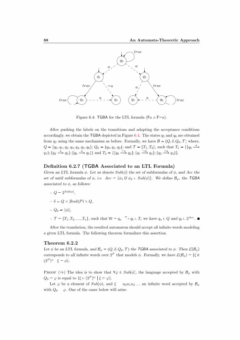
88 An Automata-Theoretic Approach
q0
q1 q2
q6q5q4q3
true
true true
aa
atrue a true
a a
Figure 6.4: TGBA for the LTL formula (Fa^ F a).
After pushing the labels on the transitions and adapting the acceptance conditionsaccordingly, we obtain the TGBA depicted in Figure 6.4. The states q5 and q6 are obtainedfrom q2 using the same mechanism as before. Formally, we have B pQ, δ,Q0, T q where,Q tq0, q1, q2, q3, q4, q5, q6u; Q0 tq0, q1, q2u; and T tT1, T2u, such that T1 ttq0
aÝÑ
q1u; tq2aÝÑ q5u; tq6
aÝÑ q5uu and T2 ttq0
aÝÑ q2u; tq1
aÝÑ q4u; tq3
aÝÑ q4uu.
Definition 6.2.7 (TGBA Associated to an LTL Formula)Given an LTL formula φ. Let us denote Subpφq the set of subformulas of φ, and Acc theset of until subformulas of φ, i.e. Acc tφ1 U φ2 P Subpφqu. We define Bφ, the TGBAassociated to φ, as follows:
- Q 2Subpφq,
- δ QBoolpP q Q,
- Q0 tφu,
- T tT1, T2, ...., Tnu, such that @t qaσÝÑ qb P Ti we have qa P Q and qb P 2Acc.
After the translation, the resulted automaton should accept all infinite words modelinga given LTL formula. The following theorem formalizes this assertion.
Theorem 6.2.2Let φ be an LTL formula, and Bφ pQ, δ,Q0, T q the TGBA associated to φ. Then LpBφqcorresponds to all infinite words over 2P that models φ. Formally, we have LpBφq tξ Pp2P qω | ξ ( φu.
Proof (ñ) The idea is to show that @ϕ P Subpφq, the language accepted by Bφ withQ0 ϕ is equal to tξ P p2P qω | ξ ( ϕu.
Let ϕ be a element of Subpφq, and ξ u0u1u2 . . . an infinite word accepted by Bφwith Q0 ϕ. One of the cases below will arise:

6.2. Representation of Büchi Automata 89
(1) ϕ p with p P P . Since Q0 tpu, and p is the only proposition that appears inQo, then we have p P σ0, thus p P ξp0q. As a result, ξ ( p (see Definition 2.3.2).
(2) ϕ g^h with g P P and h P P . We then have Q0 tg^hu, i.e. g P σ0 and h P σ0,which implies g P ξp0q ^ h P ξp0q. Thus, ξ ( g and ξ ( h. As a result, we concludeξ ( g ^ h.
(3) ϕ g _ h with g P P and h P P . We then have Q0 tg _ hu, i.e. g P σ0 or h P σ0,which implies g P ξp0q _ h P ξp0q. Thus, ξ ( g or ξ ( h. As a result, we concludeξ ( g _ h.
(4) ϕ Xg with g P P . We have Q0 tXgu and Q1 tgu. This implies that g P ξp1q.We then can say that ξ1 ( g. Hence, ξ ( Xg (see Definition 2.3.2).
(5) ϕ gUh with g P P and h P P . Applying the tableau rules, we have gUh h _ pg ^ XpgUhqq. Therefore, proving ξ ( gUh is then equivalent to provingξ ( h_ pg ^ XpgUhqq.We have
Q0 th_ pg ^ XpgUhqqu,
thus h P ξp0q
_g P ξp0q ^ g P ξp1q ^ h P ξp1q
.
i.e. ξ ( h
_ξ ( g ^ ξ1 ( g ^ ξ1 ( hq
.
We then found i 1 such that ξi ( h and @j i, ξi ( g. Hence, following Definition2.3.2, we conclude that ξ ( gUh.
Note that if g and h are elements of 2subpφq the proof can still be constructed recursivelyusing the above results. The proof of all derived operators can also be obtained fromthese results.
(ð) Let ξ u0u1u2 . . . be an infinite word modeling the formula φ. We will provethat ξ is accepted by Bφ. To do that, we need to show that @Tj P T , there exists ti P Tjthat appears infinitely often in a run of the form ρ q0
σ0ÝÑ q1σ1ÝÑ q2
σ2ÝÑ . . ., such that@i ¥ 0, ui P σi.
Let Tj be a set of transition in T . The following two facts can be established.
(i) We have seen before that if ξ ( φ, then for a subformula ϕ gUh we will also haveξ ( ϕ with Q0 ϕ.
(ii) By definition of Bφ, each element t P Tj is of the form qaσÝÑ qb where qb P Acc i.e.
qb P tgUh P Subpφqu.
Combining the facts (i) and (ii), we can say that any element of Tj will appear infinitelyoften in the run ρ, which means ρ is accepted by Bφ. Thus, ξ is accepted by Bφ.
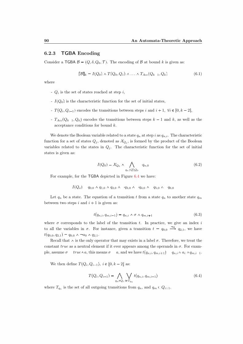
90 An Automata-Theoretic Approach
6.2.3 TGBA Encoding
Consider a TGBA B pQ, δ,Q0, T q. The encoding of B at bound k is given as:
vBwk IpQ0q ^ T pQ0, Q1q ^ . . .^ TAccpQk1, Qkq (6.1)
where
- Qi is the set of states reached at step i,
- IpQ0q is the characteristic function for the set of initial states,
- T pQi, Qi1q encodes the transitions between steps i and i 1, @i P r0, k 2s,
- TAccpQk1, Qkq encodes the transitions between steps k 1 and k, as well as theacceptance conditions for bound k.
We denote the Boolean variable related to a state qn at step i as qn,i. The characteristicfunction for a set of states Qj , denoted as XQj , is formed by the product of the Booleanvariables related to the states in Qj . The characteristic function for the set of initialstates is given as:
IpQ0q XQ0 ^©
qnPQzQ0
qn,0 (6.2)
For example, for the TGBA depicted in Figure 6.4 we have:
IpQoq q0,0 ^ q1,0 ^ q2,0 ^ q3,0 ^ q4,0 ^ q5,0 ^ q6,0
Let qn be a state. The equation of a transition t from a state qn to another state qmbetween two steps i and i 1 is given as:
tpqn,i, qm,i1q qn,i ^ σ ^ qm,i1 (6.3)
where σ corresponds to the label of the transition t. In practice, we give an index i
to all the variables in σ. For instance, given a transition t q0,0 aÝÑ q2,1, we have
tpq0,0, q2,1q q0,0 ^ a0 ^ q2,1.Recall that ^ is the only operator that may exists in a label σ. Therefore, we treat the
constant true as a neutral element if it ever appears among the operands in σ. For exam-ple, assume σ true^a, this means σ a, and we have tpqn,i, qm,i1q qn,i^ ai ^qm,i1.
We then define T pQi, Qi1q, i P r0, k 2s as:
T pQi, Qi1q ©qnPQi
ªtPTqn
tpqn,i, qm,i1q (6.4)
where Tqn is the set of all outgoing transitions from qn, and qm P Qi1.
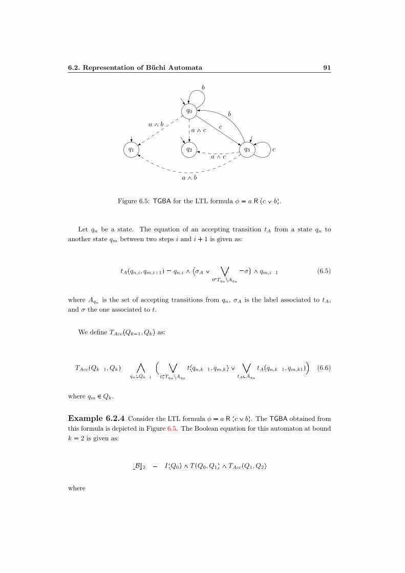
6.2. Representation of Büchi Automata 91
q0
q1 q3q2
b
c
a^ ca^ b c
a^ c
a^ b
b
Figure 6.5: TGBA for the LTL formula φ a R pc_ bq.
Let qn be a state. The equation of an accepting transition tA from a state qn toanother state qm between two steps i and i 1 is given as:
tApqn,i, qm,i1q qn,i ^σA _
ªtPTqn zAqn
σ^ qm,i1 (6.5)
where Aqn is the set of accepting transitions from qn, σA is the label associated to tA,and σ the one associated to t.
We define TAccpQk1, Qkq as:
TAccpQk1, Qkq ©
qnPQk1
ªtPTqn zAqn
tpqn,k1, qm,kq _ª
tAPAqn
tApqn,k1, qm,k1q
(6.6)
where qm P Qk.
Example 6.2.4 Consider the LTL formula φ a R pc_ bq. The TGBA obtained fromthis formula is depicted in Figure 6.5. The Boolean equation for this automaton at boundk 2 is given as:
vBw2 IpQ0q ^ T pQ0, Q1q ^ TAccpQ1, Q2q
where
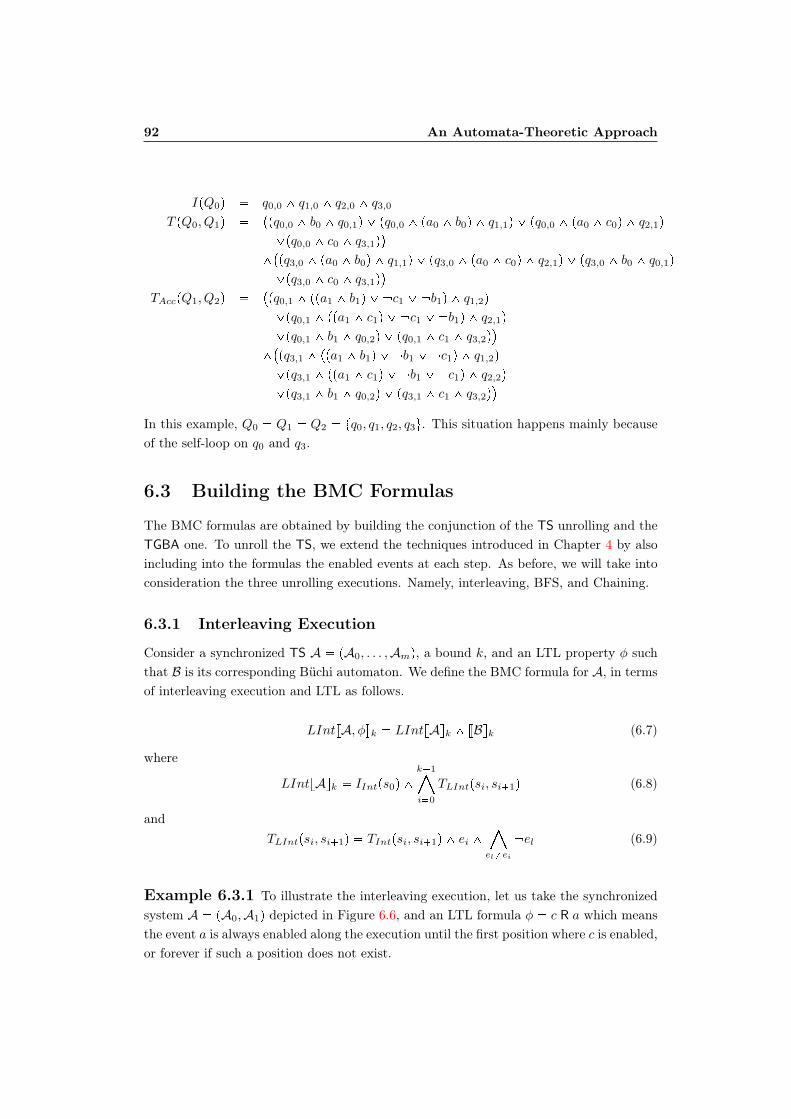
92 An Automata-Theoretic Approach
IpQ0q q0,0 ^ q1,0 ^ q2,0 ^ q3,0
T pQ0, Q1q pq0,0 ^ b0 ^ q0,1q _ pq0,0 ^ pa0 ^ b0q ^ q1,1q _ pq0,0 ^ pa0 ^ c0q ^ q2,1q
_pq0,0 ^ c0 ^ q3,1q
^pq3,0 ^ pa0 ^ b0q ^ q1,1q _ pq3,0 ^ pa0 ^ c0q ^ q2,1q _ pq3,0 ^ b0 ^ q0,1q
_pq3,0 ^ c0 ^ q3,1q
TAccpQ1, Q2q pq0,1 ^ ppa1 ^ b1q _ c1 _ b1q ^ q1,2q
_pq0,1 ^ ppa1 ^ c1q _ c1 _ b1q ^ q2,1q
_pq0,1 ^ b1 ^ q0,2q _ pq0,1 ^ c1 ^ q3,2q
^pq3,1 ^ ppa1 ^ b1q _ b1 _ c1q ^ q1,2q
_pq3,1 ^ ppa1 ^ c1q _ b1 _ c1q ^ q2,2q
_pq3,1 ^ b1 ^ q0,2q _ pq3,1 ^ c1 ^ q3,2q
In this example, Q0 Q1 Q2 tq0, q1, q2, q3u. This situation happens mainly becauseof the self-loop on q0 and q3.
6.3 Building the BMC Formulas
The BMC formulas are obtained by building the conjunction of the TS unrolling and theTGBA one. To unroll the TS, we extend the techniques introduced in Chapter 4 by alsoincluding into the formulas the enabled events at each step. As before, we will take intoconsideration the three unrolling executions. Namely, interleaving, BFS, and Chaining.
6.3.1 Interleaving Execution
Consider a synchronized TS A pA0, . . . ,Amq, a bound k, and an LTL property φ suchthat B is its corresponding Büchi automaton. We define the BMC formula for A, in termsof interleaving execution and LTL as follows.
LIntvA, φwk LIntvAwk ^ vBwk (6.7)
where
LIntvAwk IIntps0q ^k1©i0
TLIntpsi, si1q (6.8)
andTLIntpsi, si1q TIntpsi, si1q ^ ei ^
©elei
el (6.9)
Example 6.3.1 To illustrate the interleaving execution, let us take the synchronizedsystem A pA0,A1q depicted in Figure 6.6, and an LTL formula φ c R a which meansthe event a is always enabled along the execution until the first position where c is enabled,or forever if such a position does not exist.
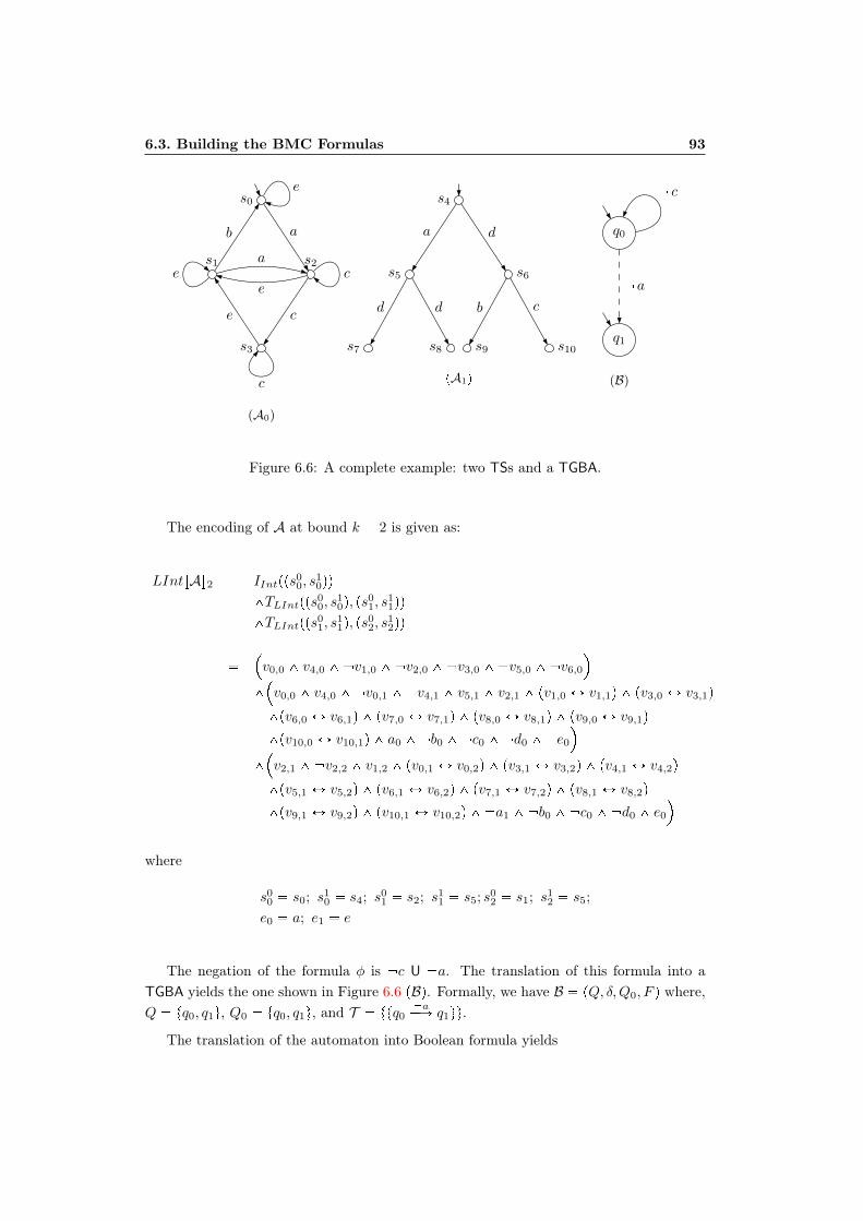
6.3. Building the BMC Formulas 93
s0
s1 s2
s3
(A0)
b
ce
a
a
ece
c
es4
s5 s6
s7 s8 s9 s10
pA1q
a
d bd
d
c
q0
q1
(B)
c
a
Figure 6.6: A complete example: two TSs and a TGBA.
The encoding of A at bound k 2 is given as:
LIntvAw2 IIntpps00, s
10qq
^TLIntpps00, s
10q, ps
01, s
11qq
^TLIntpps01, s
11q, ps
02, s
12qq
v0,0 ^ v4,0 ^ v1,0 ^ v2,0 ^ v3,0 ^ v5,0 ^ v6,0
^v0,0 ^ v4,0 ^ v0,1 ^ v4,1 ^ v5,1 ^ v2,1 ^ pv1,0 Ø v1,1q ^ pv3,0 Ø v3,1q
^pv6,0 Ø v6,1q ^ pv7,0 Ø v7,1q ^ pv8,0 Ø v8,1q ^ pv9,0 Ø v9,1q
^pv10,0 Ø v10,1q ^ a0 ^ b0 ^ c0 ^ d0 ^ e0
^v2,1 ^ v2,2 ^ v1,2 ^ pv0,1 Ø v0,2q ^ pv3,1 Ø v3,2q ^ pv4,1 Ø v4,2q
^pv5,1 Ø v5,2q ^ pv6,1 Ø v6,2q ^ pv7,1 Ø v7,2q ^ pv8,1 Ø v8,2q
^pv9,1 Ø v9,2q ^ pv10,1 Ø v10,2q ^ a1 ^ b0 ^ c0 ^ d0 ^ e0
where
s00 s0; s1
0 s4; s01 s2; s1
1 s5; s02 s1; s1
2 s5;
e0 a; e1 e
The negation of the formula φ is c U a. The translation of this formula into aTGBA yields the one shown in Figure 6.6 pBq. Formally, we have B pQ, δ,Q0, F q where,Q tq0, q1u, Q0 tq0, q1u, and T ttq0
aÝÑ q1uu.
The translation of the automaton into Boolean formula yields
94 An Automata-Theoretic Approach
vBw2 IpQ0q
^T pQ0, Q1q
^TAccpQ1, Q2q
q0,0 ^ q1,0
^pq0,0 ^ c0 ^ q0,1q _ pq0,0 ^ a0 ^ q1,1q
^pq0,1 ^ c1 ^ q0,2q _ pq0,1 ^ p a1 _ c1q ^ q1,2q
Here again we have Q0 Q1 Q2 tq0, q1u because of the self-loop on q0.The BMC equation is obtained by the conjunction of the two formulas. We have,
LIntvA, φw2 LIntvAw2 ^ vBw2.Using a SAT solver one can find a satisfying assignment for the formula at bound
k 2. We then have the following counterexample:
ps0, s4qaÝÑ ps2, s5q
eÝÑ ps1, s5q
Theorem 6.3.1Given a synchronized system A pA0, . . . ,Amq, an LTL formula φ, and a bound k. IfLIntvA, φwk is satisfiable, then A * φ.
Proof Assume that LIntvA, φwk is satisfiable, i.e. LIntvAwk ^ vBwk is satisfiable. Thisalso means that IIntps0q ^ TLIntps0, s1q ^ . . .^ TLIntpsk1, skq, which represents the en-coding of the execution from step 0 to step k, is satisfiable. Since vBwk, which representsthe encoding of the negation of the property φ at bound k, is also satisfiable, we cantherefore say that we found a path of length k from the initial state to a state where theLTL property is violated, which means we have A * φ.
Theorem 6.3.2Given a synchronized system A pA0, . . . ,Amq, an LTL formula φ, and a bound k.A * φ implies that Dk P N such that LIntvA, φwk is satisfiable.
Proof To prove this theorem, all we need to do is use the results from the proof ofTheorem 4.4.2 and replace φ into B.
6.3.2 Breadth First Search Execution
Given a synchronized system A pA0, . . . ,Amq, and a bound k, and an LTL formula φsuch that B is its corresponding Büchi automaton. We define the BMC formula for A, interms of BFS execution and LTL, as follows.
LBfsvA, φwk LBfsvAwk ^ vBwk (6.10)
6.3. Building the BMC Formulas 95
where
LBfsvAwk IBfsps0q ^k1©i0
TLBfspsi, si1q (6.11)
andTLBfspsi, si1q TBfspsi, si1q ^
©eiPEi
ei ^©
elPΣzEi
el (6.12)
Recall that Σ mj0 Σj , while Ei corresponds to the set of events that fire at step i
(see Definition 4.4.2).
Example 6.3.2 As an Example, consider the synchronized system A pA0,A1q de-picted in Figure 6.6, and the LTL formula φ c R a. The unrolling of A using the BFSmethod for k = 2 is given as:
LBfsvAw2 IBfsppS00 , S
10qq
^TLBfsppS00 , S
10q, pS
01 , S
11qq
^TLBfsppS01 , S
11q, pS
02 , S
12qq
v0,0 ^ v4,0 ^ v1,0 ^ v2,0 ^ v3,0 ^ v5,0 ^ v6,0
^v0,0 ^ v4,0 ^ v0,1 ^ v4,1 ^ v2,1 ^ v5,1 ^ v6,1 ^ pv1,0 Ø v1,1q
^pv3,0 Ø v3,1q ^ pv7,0 Ø v7,1q ^ pv8,0 Ø v8,1q ^ pv9,0 Ø v9,1q
^pv10,0 Ø v10,1q ^ a0 ^ b0 ^ c0 ^ d0 ^ e0
^v2,1 ^ v5,1 ^ v6,1 ^ v0,1 ^ v0,2 ^ v1,2 ^ v2,2 ^ v3,2 ^ v7,2 ^ v8,2
^v10,2 ^ pv4,1 Ø v4,2q ^ pv9,1 Ø v9,2q
^ a0 ^ b0 ^ c0 ^ d0 ^ e0
where
S00 ts0u; S
10 ts4u; S
01 ts0, s2u; S
11 ts5, s6u; S
02 ts0, s1, s2, s3u; S
12 ts7, s8, s10u;
E0 ta, d, eu; E1 tc, d, eu
To verify whether the system satisfy the property φ we simply build the BMC equationLBfsvA, φw2 LBfsvAw2 ^ vBw2, where vBw2 is the same as in Example 6.3.1.
We then obtain the following counterexample at bound k 2:
pts0u, ts4uqta,d,euÝÑ pts0, s2u, ts5, s6uq
tc,d,euÝÑ pts0, s1, s2, s3u, ts7, s8, s10uq
Theorem 6.3.3Given a synchronized system A pA0, . . . ,Amq, an LTL formula φ, and a bound k. IfLBfsvA, φwk is satisfiable, then A * φ.
Proof Assume that LBfsvA, φwk is satisfiable. This means LBfsvAwk ^ vBwk is satisfi-able. This implies that IBfsps0q^
k1i0 TLBfspsi, si1q is satisfiable (see equation (6.14)).
96 An Automata-Theoretic Approach
Hence, there exists a path of length k from the initial state. Since vBwk represents thenegation of the property, and since the product LBfsvAwk ^ vBwk is satisfiable, we con-clude that we found a path leading to a state where the property φ is violated. Therefore,we have A * φ.
Theorem 6.3.4Given a synchronized system A pA0, . . . ,Amq, an LTL formula φ, and a bound k.A * φ implies that Dk P N such that LBfsvA, φwk is satisfiable.
Proof Assume A * φ. This means that, using the BFS execution, we can construct apath from the initial state to a state where the property φ is violated. Assume that kis the length of that path. We then have a path s0, . . . , sk. Since si1 is reachable fromsi in one step, we can say that TBfspsi, si1q 1. Therefore, we also have IBfsps0q ^
TBfsps0, s1q ^ . . . ^ TBfspsk1, skq 1. Hence LBfsvAwk IBfsps0q ^ TLBfsps0, s1q ^
. . . ^ TLBfspsk1, skq 1 because each TLBfspsi, Si1q is an extension of TBfspsi, si1q
by simply adding the transition label into the equation, and adding the label will notchange the satisfiability of the formula. The property φ is violated at step k. Therefore,we conclude that LBfsvAwk^, vBwk is satisfiable as B represents the negation of theproperty φ.
6.3.3 Chaining
Given a synchronized system A pA0, . . . ,Amq, and a bound k, and an LTL formula φsuch that B is its corresponding Büchi automaton. We define the BMC formula for A, interms of chaining execution and LTL, as follows.
LChainvA, φwk LChainvAwk ^ vBwk (6.13)
where
LChainvAwk IChainps10q ^
k1©i0
TLChainps1i, si1q (6.14)
and
TLChainps1i, si1q TChainps
1i, si1q ^
©eiPEi
ei ^©
elPΣzEi
el (6.15)
Example 6.3.3 Let us take again the synchronized system A pA0,A1q depicted inFigure 6.6 and the LTL formula: φ c R a. The unrolling of A at bound k 2 using thechaining execution is given by the following equation:
6.4. Discussion 97
LChainvAw1 ILChainppS100 , S
110 qq
^TLChainppS100 , S
111 q, pS
01 , S
11qq
v0,0 ^ v2,0 ^ v4,0 ^ v5,0 ^ v1,0 ^ v3,0 ^ v6,0 ^ v7,0 v8,0
^ v9,0 ^ v10,0
^v0,0 ^ v2,0 ^ v4,0 ^ v5,0 ^ v4,1 ^ v2,1 ^ v5,1 ^ v0,1 ^ v1,1 ^ v6,1 ^ v7,1 ^ v8,1
^pv3,0 Ø v3,1q ^ pv9,0 Ø v9,1q ^ pv10,0 Ø v10,1q
^a0 ^ b0 ^ c0 ^ d0 ^ e0
where,
S00 ts0u; S
100 ts0, s2u; S
10 ts4u; S
110 ts4, s5u; S
01 ts0, s1u; S
11 ts6, s7, s8u;
E0 ta, d, eu
In this example we use the chaining order ra, d, es.As before, the BMC equation is obtained with the conjunction LChainvA, φw2
LChainvAw2 ^ vBw2, where vBw2 is the same as in Example 6.3.1.We obtain the following counterexample:
pts0, s2u, ts4, s5uqE0ÝÑ pts0, s1u, ts6, s7, s8uq
Theorem 6.3.5Given a synchronized system A pA0, . . . ,Amq, an LTL formula φ, and a bound k. IfLChainvA, φwk is satisfiable, then A * φ.
Proof To prove this theorem, all we need to do is use the reasoning from the proof ofTheorem 6.3.3 and change LBfs into LChain.
Theorem 6.3.6Given a synchronized system A pA0, . . . ,Amq, an LTL formula φ, and a bound k.A * φ implies that Dk P N such that LChainvA, φwk is satisfiable.
Proof The proof of this theorem is also similar to the one for Theorem 6.3.4. All weneed to do is change LBfs into LChain.
6.4 Discussion
An automata-theoretic approach offers numerous advantages when it is combined withmodel checking in general. However, it also has its drawbacks. We will discuss some ofthem in this section.
First, since the transformation algorithm itself may presents some errors, it can bedifficult sometimes to know whether the obtained automaton correctly represents the
98 An Automata-Theoretic Approach
given LTL formula. Therefore, it may be necessary to verify the transformation algorithmbeforehand or, alternatively, test several transformation techniques on the same formulaand compare the results. The work in [TH00] demonstrates how to conduct such tests.
Second, an automaton transformation algorithm has an exponential time complexityin the worst and best case [Wol02]. Still, it is practically feasible because, as mentionedearlier, most of the LTL formulas used in verification produce small automata. Onesolution of this problem is to use alternating automata [GO01], which can be generated inlinear time. It has been pointed out that finding the optimal size for a Büchi automatonis a PSPACE-hard problem [EH00].
Despite the problems mentioned above, automata-theoretic approaches have been suc-cessfully implemented into numerous model checking tools including Java PathFinder[VHBP00] developed at the NASA Ames Research Center, and SPIN [Hol97] developedby Bell Labs.
Chapter 7
Implementation
We have implemented our methods in a toolset written in C++. The tool accepts asinput transition systems and Petri nets. Although all the BMC methods we describedin Chapter 4, Chapter 5, and Chapter 6 are devoted to TS models, we have integratedin the tool some options allowing the user to perform deadlock detection for Petri nets.We have also implemented the heuristic algorithms discussed in Chapter 5 for Petri nets.Concerning the TS models, the tool can perform deadlock detection using the methoddescribed in Chapter 4, and LTL verification using the method in Chapter 6. Basically,all the major functions in the tool are initiated through command lines entered by theuser. We call the tool BMC++. We will describe it in this chapter, and show with someexamples the different tasks it can accomplish.
7.1 Different Modules
The tool has four major modules: LTL2BA, BMC, CNF translator, and solver (see Figure7.1).
7.1.1 LTL2BA
Description
If the user enters an LTL specification, it will be first translated into a Büchi automaton,as explained in Chapter 6. The LTL2BA module assumes this task. The module negatesthe formula, transforms it into NNF, and stores it as a tree structure. Then it uses thegenerated tree to build the BA.
Implementation Details
The core of this module is formed by four principal functions. Namely, a parser, an NNFtranslator, a function that builds the tree structure, and the one which generates the BA.

100 Implementation
TS PN LTL
LTL2BA Module
BMC Module
CNF Translator
Solver
Result
CEX NO CEX
Figure 7.1: BMC++ major modules.
Once the formula has been entered, the parser will parse it. If the formula is correct,then the parser will negate it. Otherwise, the process stops and the tool prompts theuser to reenter the formula. To simplify the task of the parser, the formula should beentered without space in between. Parentheses are allowed if the user prefers to put moreemphasis on the operators. Table 7.1 shows the list of the most used LTL operators andhow the user should enter them.
Table 7.1: LTL operators and their keyboard equivalents
Operator Keyboard Equivalent
!^ &_ |ñ > =
After parsing the formula, the parser will give its negation to the NNF translator,which simply applies the rules in equations (2.11) to (2.15) to create an NNF formula.Then, another function will receive the generated NNF formula and translate it into treestructure. This step is necessary because it is much more easier to handle the formula if
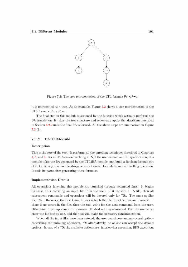
7.1. Different Modules 101
^
F F
a
a
Figure 7.2: The tree representation of the LTL formula Fa^ F a.
it is represented as a tree. As an example, Figure 7.2 shows a tree representation of theLTL formula Fa^ F a.
The final step in this module is assumed by the function which actually performs theBA translation. It takes the tree structure and repeatedly apply the algorithm describedin Section 6.2.2 until the final BA is formed. All the above steps are summarized in Figure7.3 (1).
7.1.2 BMC Module
Description
This is the core of the tool. It performs all the unrolling techniques described in Chapters4, 5, and 6. For a BMC session involving a TS, if the user entered an LTL specification, thismodule takes the BA generated by the LTL2BA module, and build a Boolean formula outof it. Obviously, the module also generate a Boolean formula from the unrolling operation.It ends its parts after generating these formulas.
Implementation Details
All operations involving this module are launched through command lines. It beginsits tasks after receiving an input file from the user. If it receives a TS file, then allsubsequent commands and operations will be devoted only for TSs. The same appliesfor PNs. Obviously, the first thing it does is fetch the file from the disk and parse it. Ifthere is no errors in the file, then the tool waits for the next command from the user.Otherwise, it prompts an error message. To deal with synchronized TSs, the user mustenter the file one by one, and the tool will make the necessary synchronization.
When all the input files have been entered, the user can choose among several optionsconcerning the unrolling operation. Or alternatively, he or she can accept the defaultoptions. In case of a TS, the available options are: interleaving execution, BFS execution,

102 Implementation
LTL Formula
Parser
NNF Translator
Tree builder
BA translator
BA
(1)
TS PN
BAParsers
Unrollers
Boolean Formulas
(2)
Figure 7.3: Details of the LTL2BA Module (1), and the BMC Module (2).
and chaining execution. Of course, they can also choose whether to check an LTL formulaor perform a deadlock detection. If the user chooses LTL formula, then the module callsa function that takes the BA generated by LTL2BA and builds a Boolean formula outof it. For the PN, the options are: interleaving execution, step execution, and processexecution. The latest two options are functions we integrated inside the tool based onthe method described in [Hel01]. Briefly put, step execution is similar to a standard BFSbut adapted to work for Petri nets, while process execution is a version of the step onethat takes only into account the shortest path among all possible step executions leadingto the same marking. Most importantly, the user can also choose whether to adopt theleap execution or not. Only deadlock detection can be performed with PNs. Figure 7.3(2) summarizes all the above steps.
Inside the tool, each TS, PN, and BA are mainly stored using a graph-like data struc-ture. The only difference is that the edges and nodes carry more information than astandard graph.
Note that, once the unrolling operation has been launched, no more input files can beentered.
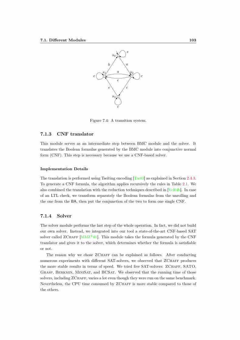
7.1. Different Modules 103
s0
s1 s2
s3
b
ce
a
a
ece
c
e
Figure 7.4: A transition system.
7.1.3 CNF translator
This module serves as an intermediate step between BMC module and the solver. Ittranslates the Boolean formulas generated by the BMC module into conjunctive normalform (CNF). This step is necessary because we use a CNF-based solver.
Implementation Details
The translation is performed using Tseiting encoding [Tse83] as explained in Section 2.4.3.To generate a CNF formula, the algorithm applies recursively the rules in Table 2.1. Wealso combined the translation with the reduction techniques described in [Vel04b]. In caseof an LTL check, we transform separately the Boolean formulas from the unrolling andthe one from the BA, then put the conjunction of the two to form one single CNF.
7.1.4 Solver
The solver module performs the last step of the whole operation. In fact, we did not buildour own solver. Instead, we integrated into our tool a state-of-the-art CNF-based SATsolver called ZChaff [MMZ01]. This module takes the formula generated by the CNFtranslator and gives it to the solver, which determines whether the formula is satisfiableor not.
The reason why we chose ZChaff can be explained as follows. After conductingnumerous experiments with different SAT-solvers, we observed that ZChaff producesthe more stable results in terms of speed. We tried five SAT-solvers: ZChaff, SATO,Grasp, Berkmin, MiniSat, and BCSat. We observed that the running time of thosesolvers, including ZChaff, varies a lot even though they were run on the same benchmark.Nevertheless, the CPU time consumed by ZChaff is more stable compared to those ofthe others.

104 Implementation
7.2 Input Formats
7.2.1 TS File format
The TS file format has three parts named header, action_names, and transitions. Inside theheader, we define the following variables: State_cnt, Transition_cnt, Initial_states whichcorrespond to the number of states, number of transitions, and initial state id respectively.Each event id and its associated name is described in the action_names part. Each linein the transitions part identifies the source, destination, and event related to a transition.Below we formalize the TS format.
Begin TS
Begin HeaderState_cnt = number of states ¡
Transition_cnt = number of transitions ¡
Initial_states = id of the initial state ¡;End Header
Begin Action_names event id1 ¡ = “ event name1 ¡” event id2 ¡ = “ event name2 ¡”. . .End Action_names
Begin Transitions source id ¡: destination id ¡, event id ¡ . . . destination id ¡, event id ¡;. . .End Transitions
End TS
Example 7.2.1 As an example, bellow we give the file for the TS depicted in Figure7.4, which is, in fact, the same as the system (A0) depicted in Figure 6.6.
Begin TS
Begin HeaderState_cnt = 4
Transition_cnt = 10
Initial_states = 0;End Header
7.2. Input Formats 105
Begin Action_names1 = “a”2 = “b”3 = “c”4 = “e”End Action_names
Begin Transitions0: 0,4 2,1;1: 0,2 1,4 2,1;2: 2,3 3,3 1,4;3: 1,4 3,3;End Transitions
End TS
7.2.2 PEP File format
For a Petri net model, we adopt the format used by the PEP tool [GB96]. Briefly put,the PEP format consist of seven principal parts. Namely, header, some default values,list of places, list of transitions, list of transition to place arcs, list of place to transitionarcs, and list of some additional information.
The PEP tool can handle many types of files, so the header is used for specifying thetype of the current file (a PEP file is identified by the keyword “PEP” in the header).Since the PEP tool is also a graphical one, some default values specifying the positions ofcertain nodes of labels in the graph are needed (e.g. position of the initial marking or theplace name). Each line in the list of places are constructed with the place identificationfollowed by some description, which may include the name of the place and its positionin the graph. The same applies for the list of transitions. Each transition to place arc isdefined by both transition and place identifications separated by the character “ ”. Theplace to transition arcs are constructed in the same way using the character “¡”. The lastpart, which is an optional one, is needed mainly for putting some graphical informationsuch as the caption of the graph. Below we formalize the PEP format.
PEPPetriBoxFORMAT_N
PL place id ¡“place description” place id ¡“place description”
106 Implementation
. . .TR transition id ¡“transition description” transition id ¡“transition description”. . .TP transition id ¡ place id ¡
transition id ¡ place id ¡
. . .PT place id ¡ ¡ transition id ¡
place id ¡ ¡ transition id ¡
. . .TX
Example 7.2.2 The following is a PEP file related to the Petri net in Figure 7.5.
PEPPetriBoxFORMAT_N
PL1“g1”M1m12“g2”3“r1”4“r2”M1m15“y1”6“y2”TR1“ta”2“tb”3“tc”4“td”TP1 1
1 4
2 5
3 3
3 2
4 6
PT

7.3. Important commands 107
g1
y1
r2
r1
y2
g2
tb
tc
ta
td
Figure 7.5: A Petri net.
1 ¡ 2
2 4
3 1
4 3
5 3
6 1
TX“Example net”
The notation “M1m1” next to the description of places g1 and r2 means that theseplaces have the initial markings and each of them has one token. The keyword TX identifiesthe last part in the file.
7.3 Important commands
Almost all the major operations in the tool are launched through command lines. Theseoperations includes reading the input files, the BMC itself, reading the LTL formula. Inthis section, we will briefly describe the most important commands available in the tool.
read_pn
Usage: read_pn PN filename ¡
Description: Opens the PN model given as argument.

108 Implementation
read_ts
Usage: read_ts TS filename ¡
Description: Opens the TS model given as argument.
enable_leap
Usage: enable_leap leapMethod ¡
Description: Enables the leap options during a BMC operation for Petri nets.This command should have, as an argument, one of the leap methods listed below.
Arguments: interpolation ¡ use the interpolation method log ¡ use the logarithmic method.
enable_chaining
Usage: enable_chaining roptionsDescription: Enables chaining during a BMC operation.Options: c use causality for ordering the events.
If no option is given the event will be chosen randomly.
go_bmc
Usage: go_bmc rbmcLengthsDescription Perform a BMC computation. If no length is given, the tool will stop at
length 10. By default, chaining is not used for TS models.
help
Usage: help rcommandNamesDescription Gives a description of the command given as argument. If no specific
command is given, the tool will simply list all available commands
set_default
Usage: set_defaultDescription: Resets the tool to the default configuration.
source
Usage: source filename ¡
Description: Runs all commands written inside the file given as argument.
reset
Usage: resetDescription: Resets the BMC session and reinitialize all variables.
A BMC session launched after this command will start from bound 1.

7.3. Important commands 109
Note that, there exist other commands than the ones listed above. To know them theuser needs only to issue the command help.

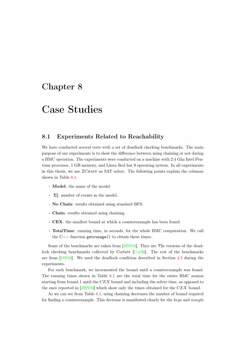
Chapter 8
Case Studies
8.1 Experiments Related to Reachability
We have conducted several tests with a set of deadlock checking benchmarks. The mainpurpose of our experiments is to show the difference between using chaining or not duringa BMC operation. The experiments were conducted on a machine with 2.4 Ghz Intel Pen-tium processor, 1 GB memory, and Linux Red hat 9 operating system. In all experimentsin this thesis, we use ZChaff as SAT solver. The following points explain the columnsshown in Table 8.1.
- Model: the name of the model.
- |Σ|: number of events in the model.
- No Chain: results obtained using standard BFS.
- Chain: results obtained using chaining.
- CEX: the smallest bound at which a counterexample has been found.
- TotalTime: running time, in seconds, for the whole BMC computation. We callthe C++ function getrusage() to obtain these times.
Some of the benchmarks are taken from [JHN03]. They are TSs versions of the dead-lock checking benchmarks collected by Corbett [Cor96]. The rest of the benchmarksare from [MR90]. We used the deadlock condition described in Section 4.5 during theexperiments.
For each benchmark, we incremented the bound until a counterexample was found.The running times shown in Table 8.1 are the total time for the entire BMC sessionstarting from bound 1 until the CEX bound and including the solver time, as opposed tothe ones reported in [JHN03] which show only the times obtained for the CEX bound.
As we can see from Table 8.1, using chaining decreases the number of bound requiredfor finding a counterexample. This decrease is manifested clearly for the keys and mmgts
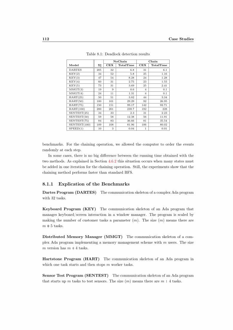
112 Case Studies
Table 8.1: Deadlock detection results
NoChain Chain
Model |Σ| CEX TotalTime CEX TotalTime
DARTES 205 32 6.8 31 6.1KEY(2) 34 52 5.8 25 1.16KEY(3) 47 54 8.28 24 1.28KEY(4) 60 31 2.75 23 1.55KEY(5) 73 31 3.69 25 2.41MMGT(3) 19 9 0.6 4 0.1MMGT(4) 24 11 1.31 4 0.1HART(25) 50 51 3.82 44 3.34HART(50) 100 101 29.29 92 26.95HART(75) 150 151 99.17 142 92.71HART(100) 200 201 239.7 192 228SENTEST(25) 34 33 2.3 31 2.23SENTEST(50) 59 58 12.38 56 11.91SENTEST(75) 84 83 36.66 81 35.54SENTEST(100) 109 108 81.96 106 80.02SPEED(1) 10 3 0.04 1 0.01
benchmarks. For the chaining operation, we allowed the computer to order the eventsrandomly at each step.
In some cases, there is no big difference between the running time obtained with thetwo methods. As explained in Section 4.6.2 this situation occurs when many states mustbe added in one iteration for the chaining operation. Still, the experiments show that thechaining method performs faster than standard BFS.
8.1.1 Explication of the Benchmarks
Dartes Program (DARTES) The communication skeleton of a complex Ada programwith 32 tasks.
Keyboard Program (KEY) The communication skeleton of an Ada program thatmanages keyboard/screen interaction in a window manager. The program is scaled bymaking the number of customer tasks a parameter (m). The size (m) means there arem 5 tasks.
Distributed Memory Manager (MMGT) The communication skeleton of a com-plex Ada program implementing a memory management scheme with m users. The sizem version has m 4 tasks.
Hartstone Program (HART) The communication skeleton of an Ada program inwhich one task starts and then stops m worker tasks.
Sensor Test Program (SENTEST) The communication skeleton of an Ada programthat starts up m tasks to test sensors. The size (m) means there are m 4 tasks.
8.1. Experiments Related to Reachability 113
Table 8.2: Comparison with NuSMV
Chain NuSMVpBMCq
Model |Σ| CEX TotalTime CEX TotalTime
DARTES 205 31 6.1 32 1111KEY(2) 34 25 1.16 60 4076KEY(3) 47 24 1.28 64 4498KEY(4) 60 23 1.55 64 5446KEY(5) 73 25 2.41 64 2960MMGT(3) 19 4 0.1 10 922MMGT(4) 24 4 0.1 12 1107HART(50) 100 92 26.95 >100 117HART(100) 200 192 228 >200 986
Speed Regulation Program (SPEED) The communication skeleton of an Ada pro-gram with 10 tasks that monitor and regulate the speed of a car.
8.1.2 Comparison with the Tool NuSMV
We have also conducted some experiments comparing the results we obtained above withthe state-of-the-art model checking tool NuSMV. The tool can perform BDD-based modelchecking and BMC. We compared our results using the BMC option in the tool. Sincethe best performances we obtained in the experiments in Table 8.1 are related to thechaining execution, we compared only the NuSMV results with the chaining execution asseen in Table 8.2. The time reported for the NuSMV BMC operations are the sum ofeach execution time from bound 0 to the CEX bound. We were not able to perform thecomparison with all the benchmarks because only a few of the Corbett benchmarks areavailable in the NuSMV format. However, we believe that the results shown in Table 8.2gives an idea on how the missing benchmarks would perform with the tool NuSMV. Toperform the NuSMV BMC operations we use the following commands:
set input_file filename ¡;set sat_solver zchaff;go_bmc;check_ltlspec_bmc -p “G (Live)” -k 50 -l X;quit;
The command set input_file provides the input file related to the current benchmark.set sat_solver defines what SAT solver to use during the BMC operation. In our case,we use ZChaff. The command go_bmc configures the systems for BMC. The commandcheck_ltlspec_bmc -p “G (Live)” -k 50 -l X checks whether the given property holds alongthe execution up to the given bound which is 50 in this particular example. In our case,the property is defined as an LTL formula “G (Live)” where live is a predicate that evalu-ates to true iff some action can be executed in the reached state. The last portion of the
114 Case Studies
command -l X says we are interested only in non-loop executions during the search forcounterexample.
In Table 8.2 NuSMVpBMCq gives the results from NuSMV BMC. For all of theHARTs benchmarks, we did not find a counterexample using the NuSMV tool. We reportonly the results from HART(50) and HART(100) for which we limit the search respectivelyat bound 100 and 200.
8.2 Experimental Results Related to LTL
We took five problems from the literature, namely gas station, bakery algorithm, readers-writers, sleeping barber, and leader election protocol. As explained in [ACL05, GG08b],choosing what benchmarks to use is no easy feat, especially when it comes to asynchronousconcurrent systems. Furthermore, the tasks become much more complex if we try to com-pare the method with other implementations. We will describe each of these benchmarksin the following subsections.
8.2.1 Gas Station
The gas station problem [PDH99, HL85] consists of simulating a self-service gas stationwith an operator, a number of pumps and customers. When a customer arrives, she firstprepays the operator to be able to fill from a specific pump. The operator then activatesthe pump, assigned an ID to the customer, and pass it through a queue associated withthe pump. Only after successful ID verification can a customer start using a pump. Whenthe customer is done, the pump passes the charge back to the operator, who charges thecustomer and returns the change, if any. The whole service is performed in a first-in-first-out manner.
8.2.2 Bakery Algorithm
The bakery algorithm [BGR95, Bul00, BB06, BGP99] deals with the mutual exclusionproblem for n processes P1, . . . , Pn that want to access a shared critical section of a code.Each process Pi has a shared register readable by the other processes but writable onlyby Pi. A natural number ni is associated to each register. Initially, all ni p1 ¤ i ¤ nq areset to zero. When a process Pi wants to access the critical section, it gives its ni a valuegreater than all nj pj iq. Then Pi keeps reading the registers of the other process Pjand wait until nj 0 or nj ¡ ni or nj ni ^ j ¡ i. Then Pi enters the critical section.Once it leaves the critical section, Pi resets the value of ni to zero.
8.2.3 Readers-writers Problem
The readers-writers problem [Bul00, CHP71] is a typical problem in concurrency. Itconcerns the situation in which many processes must access a shared memory at the same
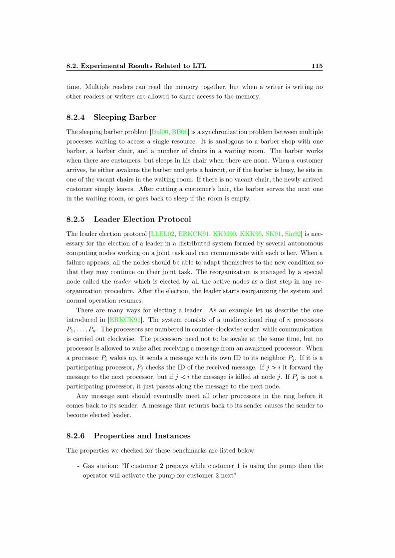
8.2. Experimental Results Related to LTL 115
time. Multiple readers can read the memory together, but when a writer is writing noother readers or writers are allowed to share access to the memory.
8.2.4 Sleeping Barber
The sleeping barber problem [Bul00, BB06] is a synchronization problem between multipleprocesses waiting to access a single resource. It is analogous to a barber shop with onebarber, a barber chair, and a number of chairs in a waiting room. The barber workswhen there are customers, but sleeps in his chair when there are none. When a customerarrives, he either awakens the barber and gets a haircut, or if the barber is busy, he sits inone of the vacant chairs in the waiting room. If there is no vacant chair, the newly arrivedcustomer simply leaves. After cutting a customer’s hair, the barber serves the next onein the waiting room, or goes back to sleep if the room is empty.
8.2.5 Leader Election Protocol
The leader election protocol [LLEL02, ERKCK91, KKM90, KKK95, SK91, Sin92] is nec-essary for the election of a leader in a distributed system formed by several autonomouscomputing nodes working on a joint task and can communicate with each other. When afailure appears, all the nodes should be able to adapt themselves to the new condition sothat they may continue on their joint task. The reorganization is managed by a specialnode called the leader which is elected by all the active nodes as a first step in any re-organization procedure. After the election, the leader starts reorganizing the system andnormal operation resumes.
There are many ways for electing a leader. As an example let us describe the oneintroduced in [ERKCK91]. The system consists of a unidirectional ring of n processorsP1, . . . , Pn. The processors are numbered in counter-clockwise order, while communicationis carried out clockwise. The processors need not to be awake at the same time, but noprocessor is allowed to wake after receiving a message from an awakened processor. Whena processor Pi wakes up, it sends a message with its own ID to its neighbor Pj . If it is aparticipating processor, Pj checks the ID of the received message. If j ¡ i it forward themessage to the next processor, but if j i the message is killed at node j. If Pj is not aparticipating processor, it just passes along the message to the next node.
Any message sent should eventually meet all other processors in the ring before itcomes back to its sender. A message that returns back to its sender causes the sender tobecome elected leader.
8.2.6 Properties and Instances
The properties we checked for these benchmarks are listed below.
- Gas station: “If customer 2 prepays while customer 1 is using the pump then theoperator will activate the pump for customer 2 next”
116 Case Studies
Table 8.3: LTL checking results
Models Bound Time CEX
4g 120 4.45 No2b 120 3.1 No4b 120 4.9 No2rw 1 0.01 Yes4rw 1 0.01 Yes8l 36 4.15 Yes10s 120 6.22 No
LTL: GppfillCustomer1^prepayCustomer2q Ñ p activate1U pactivate2_G activate1qq
- Bakery: “Only one process can enter the critical section”
LTL: G pcriticalSection1^ criticalSection2^ . . .q
- Readers-writers: “At any time, there must be at least one writer writing and at leastone reader reading.”
LTL: Gppw1_ w2_ . . .q ^ pr1_ r2_ . . .qq
- Leader election: “If process 1 is the elected processor then it will be the only onethat enter into the elected state”
LTL: GpleaderP1 Ñ pleaderP2_ leaderP3_ . . .qq
- Sleeping Barber: “The barber cut one person at a time”
LTL: G pcustomer1^ customer2^ . . .q
For the gas station problem we used an instance with four customers, one pump andone queue (g4). For the bakery algorithm we used a version with two processors (2b) andanother with four processors (4b). We did the same with readers-writers (2rw and 4rw).We used a ring with eight nodes for the leader election (8l), and finally a model with tencustomers for the sleeping barber (10s).
As before, the experiments were conducted on a machine with 2.4 Ghz Intel Pentiumprocessor, 1 GB memory, and Fedora 10 operating system. The following points explainthe columns shown in Table 8.3.
- Models: the model instances as explained above,
- Bound: the deepest bound used for the tests,
- Time: running time, in seconds, for the whole BMC computation starting frombound 1 including the solver time.

8.3. Experiments Related to Leap 117
Table 8.4: Comparison of leap and standard BMC
Leap BMC
Model |P| |T| Max L. Standard BMC Log. Inter.
KEY(2) 94 92 36 836.95 6.49 13.52KEY(3) 129 133 36 2458.89 5.64 17.36KEY(4) 164 174 36 4231.53 9.96 26.71DEMUX(16) 352 258 ¡80 153.58 16.89 20.86REG(4) 77 96 ¡50 490.72 29.33 11.93REG(8) 153 184 ¡20 342.61 57.45 100.32SDL-ARQ 163 96 ¡44 5313.13 1446.14 1423.41FIR-4-A1M1
1394 1131 ¡80 8043.52 1526.8 690.7
FIR-4-A2M2
1444 1158 ¡80 9478.42 2067.2 972.18
IIR-A1M1 576 476 ¡80 1513.35 188.71 188.09IIR-A2M2 544 437 ¡80 1534.71 277.99 221.1LF2 315 267 ¡90 11131.23 4037.65 3618.57
- CEX: a “yes” or “no” column that indicates whether a counterexample has beenfound or not at the current bound.
For each benchmark, we incremented the bound little by little. We limited the search atbound 120 for this experiments. For the properties we checked we found counterexamplesonly for the readers-writers and leader election problems.
8.3 Experiments Related to Leap
As usual, the experiments were conducted on a machine with 2.4 Ghz Intel Pentiumprocessor, 1 GB memory, and Linux Red hat 9 operating system. As mentioned in Remark5.3.1 we conducted the leap experiments using Petri net models. The Keys benchmarksare taken from the Petri net versions of Corbett’s case studies [Cor96]. Demux, Regs,and sdl-arq are converted from STG benchmarks, while firs, iirs, and lf belong to theSTG benchmark family used in [YOM04]. We performed deadlock detection using thedeadlock condition described in [Hel01]. For the standard BMC the method used is similarto a standard BFS execution but adapted to work for Petri nets. The following pointsexplain the columns shown in Table 8.4.
- Model: the name of the model.
- |P|: number of places in the model.
- |T|: number of transitions in the model.
- Max L.: maximal length of a BMC session. A number preceded by “¡” indicatesthat no counterexample has been found up to this bound.
118 Case Studies
- Standard BMC: total CPU time, in seconds, for the whole BMC computationfor standard BMC, starting from bound 1 until the maximal length, including theSAT-solver’s time. We call the C++ function getrusage() to obtain these times.
- Leap BMC: the same as in Standard BMC but for the leap approach. Here thebound starts from fixLeap.
- Log.: results obtained when using the logarithmic jumping method.
- Inter.: results obtained when using the interpolation/extrapolation method.
Our goal is to show the efficiency of the big leap approach compared with standardBMC. Table 8.4, shows the results we obtained from the comparison. We report therunning time obtained using the two jumping methods. As you can see, in general, theinterpolation method runs slower than the logarithmic one. Still, both methods outper-form the standard BMC approach.
8.4 Example of a Leap Execution
Below is a detailed explanation of a big leap execution using Algorithm 5.2. It consists ofthe result obtained in Table 8.4, column 6, last line, with the lf2 benchmark.
We used the following parameters:
- Model: lf2
- BMC method: big leap
- Jumping method: logarithmic
- Fix leap = 4
- minC = 1 sec.
- midC = 60 sec.
- maxC = 150 sec.
- limC = 1 hr.
- Maximum iteration for minC = 9
- Maximum BMC Length = 90
We obtained the following results. (Explanation is given after the whole results.)
- leap = 4
Solving time: 0
No counterexample found with bound 4
8.4. Example of a Leap Execution 119
- leap = 4
Solving time: 0.01
No counterexample found with bound 8
- leap = 4
Solving time: 0.04
No counterexample found with bound 12
- leap = 4
Solving time: 0.06
No counterexample found with bound 16
- leap = 4
Solving time: 0.12
No counterexample found with bound 20
- leap = 4
Solving time: 0.17
No counterexample found with bound 24
- leap = 4
Solving time: 0.41
No counterexample found with bound 28
- leap = 4
Solving time: 0.44
No counterexample found with bound 32
- leap = 4
Solving time: 0.68
No counterexample found with bound 36
120 Case Studies
- leap = 20
Solving time: 3.04
No counterexample found with bound 56
- leap = 24
Solving time: 140
No counterexample found with bound 80
- leap = 6
Solving time: 291.6
No counterexample found with bound 86
- leap = 4
Solving time: 3601.08
No counterexample found with bound 90
- Total CPU time: 4037.65
The execution starts with leap 4 and continues this way until bound 36. During thisperiod, we have solvingT ime minC. At this bound, the algorithm computes a new leapvalue because the maximum iteration forminC is reached (see explanation in Section 5.4).The leap becomes leap 4 log2p36q 20, which corresponds to the formula used forthe second condition in the algorithm. At bound 56, the algorithm still uses this formulabecause the solving time is still less than midC, so we have leap 4 log2p56q 24.At bound 80, we reach the situation where midC ¤ solvingT ime maxC, then thealgorithm computes another new leap value, which is leap log2p80q 6. maxC issurpassed at bound 86, and the leap becomes 4 again. The algorithm stops at bound 90because the maximum BMC Length is reached.

Chapter 9
Conclusions and Future Work
9.1 Conclusions
In this dissertation, the research goal has been to develop efficient verification techniquesfor asynchronous concurrent systems. We focused on BMC using synchronized productsof transition systems (TSs) as a model. Our idea is to replace the standard interleavingtechnique with techniques based on the breadth-first search (BFS) execution. Whileinterleaving techniques allow us only to fire one event at a time, with breadth-first searchwe can fire multiple events together, which is really helpful when dealing with concurrentsystems because it reduces the number of paths to be explored during the operation.
We have shown that combining BFS with chaining traversal can improve the BMCperformance. The main objective in chaining is to reduce the number of the executionsteps by firing the enabled events following a predefined order. The efficacy of chainingdepends to a large extent on the chosen event order. It is, therefore, important to use theright event order during a chaining operation.
To increase the speed of a BMC operation, we have proposed a method based on leap.That is, we do not call the SAT solver at every single bound but at intervals. The numberof bounds to be skipped is determined by the leap values. Normally, skipping boundssuggest that some counterexamples could be missed if they appeared in some of thosebounds that have been skipped. To cope with this problem, we introduced a method thatallows us to catch all errors if they exist all along the execution. We also introduced twojumping heuristics that can be used for selecting the bounds to be skipped. Experiencehave shown that the leap approach greatly improve the speed of the operation.
All the methods above are built for checking reachability properties. We have also pro-posed a method for verifying other properties written with the logic LTL. The method isbased on the so-called automata-theoretic approach in which the LTL specification is firsttranslated into Büchi automata before creating a Boolean formula. The advantage of us-ing an automata as an intermediate step is that it is simpler to generate a Boolean formulafrom the automata and to combine it with the one generated form the TS unrolling.
122 Conclusions and Future Work
We have implemented all these methods in a BMC toolset that can perform deadlockdetection, and also can check LTL specifications. We conducted some experiments usingthe tool and compare our results with the state-of-the-art NuSMV tool. The methodsshow promise in the experimental results conducted using the tool.
9.2 Future Work
The following points summarizes possible future research directions related to this work.
Path compression For the methods devoted to reachability properties, combiningthem with path compression techniques such as the one in [KLY02] may bring someimprovements. This idea could be interesting, because it will diminish the path to besearched, thus making the BMC formula even smaller.
Event ordering To improve the chaining method, the focus should be on the eventordering since a good event order is key to the success of the operation. In this work, wehave used only one event ordering technique which works better for some kinds of systems.However, it is crucial to use a method guaranteed to work with any type of system.
Reduction techniques For the leap approach, integrating some reduction techniques,such as the ones in [Ber85, PRCB94, ES01], prior to the actual BMC computation couldbe interesting. This is useful especially when dealing with large systems since this reducesthe size of the model, thus reduces the number of bounds to be explored, and decreaseseven further the execution time during search for counterexamples.
Checking CTL formulas It is also interesting to improve the encoding so that it canbe used not only for checking LTL formulas, but other types of temporal logic such asCTL for instance.

Bibliography
[ABE00] P.A. Abdulla, P. Bjesse, and N. Eén. Symbolic reachability analysis based onSAT solvers. In S. Graf and M. Schwartzbach, editors, Proc. of the 6th Int.Conf. on Tools and Algorithms for the Construction and Analysis of Systems(TACAS’00), volume 1785 of LNCS, pages 411–425, Berlin, Germany, March2000. Springer-Verlag.
[ÁBKS05] E. Ábrahám, B. Becker, F. Klaedtke, and M. Steffen. Optimizing boundedmodel checking for linear hybrid systems. In R. Cousot, editor, Proc. of the6th Int. Conf. on Verification, Model Checking, and Abstract Interpretation(VMCAI 2005), volume 3385 of Lecture Notes in Computer Science, pages396–412, Paris, France, January 17-19 2005. Springer-Verlag.
[ACA78] T. Agerwala and Y. Choed-Amphai. A synthesis rule for concurrent systems.In Proc. of the 15th conf. on Design Automation, pages 305–311, Las Vegas,Nevada, United States, June 1978. IEEE Press.
[ACKS02] G. Audemard, A. Cimatti, A. Kormilowicz, and R. Sebastiani. Boundedmodel checking for timed systems. In Proc. of the 22nd Joint Int. Conf. onFormal Techniques for Networked and Distributed Systems (FORTE 2002),volume 22 of LNCS, pages 243–259, Houston, Texas, U.S., November 2002.Springer-Verlag.
[ACL05] D-A. Atiya, N. Catano, and G. Lüttgen. Towards a benchmark for modelcheckers of asynchronous concurrent systems. Technical report, Universityof Warwick, U.K., 2005.
[AD94] R. Alur and D.L. Dill. A theory of timed automata. Theoretical ComputerScience, 126(2):183–235, 1994.
[ADA05] N. Amla, X. Du, A.Kuehlmann, R.P. Kurshan, and K.L. McMillan. An anal-ysis of SAT-based model checking techniques in an industrial environment.In D. Borrione and W. J. Paul, editors, Proc. of the 13th Int. Conf. on Cor-rect Hardware Design and Verification Methods (CHARME 2005), volume3725 of Lecture Notes in Computer Science, pages 254–268, Saarbrücken,Germany, October 2005. Springer-Verlag.

124 BIBLIOGRAPHY
[Ade97] A. Adelman. The mathematics of the pentium bug. SIAM Review,39(March):54–67, 1997.
[AEF05] R. Armoni, S. Egorov, R. Fraer, D. Korchemny, and M. Vardi. EfficientLTL compilation for SAT-based model checking. In Proc. of the Int. Conf.on Computer-Aided Design (ICCAD’05), pages 877–884. IEEE ComputerSociety, November 2005.
[AH04] R Arora and M. S. Hsiao. Enhancing SAT-based bounded model checkingusing sequential logic implications. In Proc. of the 17th Int. Conf. on VLSIDesign, pages 784–787, 2004.
[ÁHBS06] E. Ábrahám, M. Herbstritt, B. Becker, and Martin Steffen. Bounded modelchecking with parametric data structures. In Proc. of the 4th Int. workshopon Bounded Model Checking (BMC’06), Seattle,Washington, U.S., August15 2006. Elsevier Science B.V.
[AKMM03] N. Amla, R. Kurshan, K. McMillan, and R. Medel. Experimental analysis ofdifferent techniques for bounded model checking. In H. Garavel and J. Hat-cliff, editors, Proc. of the 9th Int. Conf. on Tools and Algorithms for theConstruction and Analysis of Systems (TACAS’03), volume 2619 of LNCS,pages 34–48. Springer-Verlag, April 2003.
[Arn94] A. Arnold. Finite Transition Systems. Masson, Paris, 1994.
[AS97] M. Abramovici and D.G. Saab. Satisfiability on reconfigurable hardware. InProc. of the 7th Int. Workshop on Field-Programmable Logic and Applica-tions, volume 1304 of Lecture Notes in Computer Science, pages 448–456.Springer-Verlag, 1997.
[AS06] M. Awedh and F. Somenzi. Termination criteria for bounded model check-ing: extensions and comparison. Electronic Notes in Theoretical ComputerScience, 144(1):51–66, 2006.
[BB04] C. Barrett and S. Berezin. CVC Lite: A new implementation of the coop-erating validity checker. In Proc. of the 16th Int. Conf. on Computer AidedVerification (CAV’2004), volume 3114 of Lecture Notes in Computer Science,pages 515–518, Boston, Massachusetts, U.S., July 2004. Springer-Verlag.
[BB06] C. Bartzis and T. Bultan. Efficient BDDs for bounded arithmetic constraints.Int. Journal on Software Tools for Technology Transfer, 8(1):26–36, 2006.
[BBC05] M. Bozzano, R. Bruttomesso, A. Cimatti, T. Junttila, P. van Rossum,S. Schulz, and R. Sebastiani. The MathSAT 3 system. In RobertNieuwenhuis, editor, Proc. of the 20th Int. Conf. on Automated Deduction(CADE’05), volume 3632 of Lecture Notes in Computer Science, pages 315–321, Tallinn, Estonia, July 2005. Springer-Verlag.
BIBLIOGRAPHY 125
[BBF99] B. Bérard, M. Bioit, A. Finkel, F. Latoussinie, A. Petit, L. Petrucci, Ph.Schnoebelen, and P. Mckenie. Systems and software verification. Springer-Verlag, 1999.
[BC00] P. Bjesse and K. Claessen. SAT-based verification without state space traver-sal. In W.A. Hunt Jr. and S.D. Johnson, editors, Proc. of. the 3rd Int. Conf.on Formal Methods in Computer-Aided Design, volume 1954 of Lecture Notesin Computer Science, pages 372–389. Springer-Verlag, November 2000.
[BC03] M. Benedetti and A. Cimatti. Bounded model checking for past LTL. InH. Garavel and J. Hatcliff, editors, Proc. of the 9th Int. Conf. on Toolsand Algorithms for the Construction and Analysis of Systems (TACAS’03),volume 2619 of LNCS, pages 18–33, Warsaw, Poland, April 2003. Springer-Verlag.
[BCC03] A. Biere, A. Cimatti, E.M. Clarke, O. Strichman, and Y. Zhu. Boundedmodel checking. Advances in computer sciences, 58, 2003.
[BCCZ99] A. Biere, A. Cimatti, E. Clarke, and Y. Zhu. Symbolic model checkingwithout BDDs. In Proc. of the Int. Conf. on Tools and Algorithms for theConstruction and Analysis of Systems (TACAS’99), volume 1579 of LectureNotes in Computer Science, pages 193–207. Springer-Verlag, March 1999.
[BCM90] J.R. Burch, E.M. Clarke, K.L. McMillan, D.L. Dill, and J. Hwang. Symbolicmodel checking: 1020 states and beyond. In Proc. of the 5th Annual IEEESymposium on Logic in Computer Science, pages 1–33, Washington, D.C.,1990. IEEE Computer Society Press.
[BCRZ00] A. Biere, E. Clarke, R. Raimi, and Y. Zhu. Verifying safety properties of aPowerPC using symbolic model checking without BDDs. In Proc. of the Int.Conf. on Formal Methods in Computer Aided Design, volume 1633 of LectureNotes in Computer Science, pages 60–71. Springer-Verlag, November 2000.
[BDL96] C. Barrett, D. Dill, and J. Levitt. Validity checking for combinations oftheories with equality. In M. Srivas and A. Camilleri, editors, Proc. of the1st Int. Conf. on Formal Methods in Computer Aided Design (FMCAD’96),volume 1166 of Lecture Notes in Computer Science, pages 187–201, PaloAlto, California, U.S., November 1996. Springer-Verlag.
[BdMS07] C. Barrett, L. de Moura, and A. Stump. Design and results of the 2nd an-nual satisfiability modulo theories competition (SMT-COMP 2006). FormalMethods in System Design, 31(3):221–239, 2007.
[BE77] J. Baer and C.S. Ellis. Model, design, and evaluation of a compiler for aparallel processing environment. IEEE Transaction on Software Engineering,3(6):394–405, 1977.
126 BIBLIOGRAPHY
[Ber85] G. Berthelot. Checking properties of nets using transformation. In Advancesin Petri Nets, covers the 6th European Workshop on Applications and Theoryin Petri Nets, volume 222 of Lecture Notes in Computer Science, pages 19–40, Espoo, Finland, June 1985. Springer-Verlag.
[BGP99] T. Bultan, R. Gerber, and W. Pugh. Model-checking concurrent systemswith unbounded integer variables: symbolic representations, approxima-tions, and experimental results. ACM Transactions on Programming Lan-guages and Systems (TOPLAS), 21(4):747–789, 1999.
[BGR95] E. Börger, Y. Gurevich, and D. Rosenzweig. The bakery algorithm: yetanother specification and verification. pages 231–243, 1995.
[BHJ06] A. Biere, K. Heljanko, T. A. Junttila, T. Latvala, and V. Schuppan. Linearencodings of bounded LTL model checking. Logical Methods in ComputerScience, 2(5:5):1–64, 2006.
[BHSV96] R.K. Brayton, G.D. Hachtel, A. Sangiovanni-Vincentelli, F. Somenzi,A. Aziz, S.T. Cheng, S. Edwards, S. Khatri, Y. Kukimoto, A. Pardo,S. Qadeer, R.K. Ranjan, S. Sarwary, T.R. Shiple, G. Swamy, and T. Villa.VIS: a system for verification and synthesis. In R. Alur and T.A. Hen-zinger, editors, Proc. of. the 8th Int. Conf. on Computer Aided Verification(CAV’96), volume 1102 of Lecture Notes in Computer Science, pages 428–432, New Brunswick, NJ, U.S., July 1996. Springer-Verlag.
[BK86] C.L. Beck and B.H. Krogh. Models for simulation and discrete control ofmanufacturing systems. In Proc. of the IEEE Int. Conf. on Robotics and Au-tomation, pages 305–310, San Francisco, U.S., 1986. IEEE Computer SocietyPress.
[BK02] F. Bause and P. Kritzinger. Stochastic Petri nets – An introduction to thetheory (2nd edition). Vieweg Verlag, 2002.
[BK04] J. Baumgartner and A. Kuehlmann. Enhanced diameter bounding via struc-tural transformation. In Proc. of. the Conf. Design Automaton and Test inEurope (DATE’2004), pages 36–41, 2004.
[BKA02] J. Baumgartner, A. Kuehlmann, and J. Abraham. Property checking viastructural analysis. In E. Brinksma and K. G. Larsen, editors, Proc. of the14th Int. Conf. on Computer Aided Verification, (CAV 2002), volume 2404 ofLecture Notes in Computer Science, pages 151–165, Copenhagen, Denmark.,July 2002. Springer-Verlag.
[BLM01] P. Bjesse, T. Leonard, and A. Mokkedem. Finding bugs in Alpha micropro-cessor using satisfiability solvers. In Proc. of the 13th Int. Conf. on Computer
BIBLIOGRAPHY 127
Aided Verification (CAV’2001), volume 2102 of Lecture Notes in ComputerScience, pages 454–464. Springer-Verlag, 2001.
[BLP95] J. Bormann, J. Lohse, and M. Payer. Model checking in industrial hardwaredesign. In Proc. of the 32th Int. Conf. on Design Automation (DAC’95),pages 298–303, San Fransisco, California, U.S., June 1995.
[BM86] G. Bruno and G. Marchetto. Process-translatable Petri nets for the rapidprototyping of process control systems. IEEE Transaction on Software En-gineering, 12(2):346–357, 1986.
[Bry86] R.E. Bryant. Graph-based algorithms for boolean function manipulations.IEEE Transactions on Computers, 35(8):677–691, 1986.
[BT82] G. Berthelot and R. Terrat. Petri nets theory for the correctness of proto-cols. In C.A. Sunshine, editor, Proc. of the IFIP WG6.1 2nd Int. Workshopon Protocol Specification, Testing and Verification (PSTV), pages 325–342,Idyllwild, CA, U.S., 1982. North-Holland.
[Bul00] T. Bultan. Bdd vs. constraint-based model checking: an experimental evalu-ation for asynchronous concurrent systems. In S. Graf and M. Schwartzbach,editors, Proc. of the 6th Int. Conf. on Tools and Algorithms for the Construc-tion and Analysis of Systems (TACAS’00), volume 1785 of LNCS, pages441–455, Berlin, Germany, March 2000. Springer-Verlag.
[BW03] F. Bacchus and J. Winter. Effective preprocessing with hyper-resolutionand equality reduction. In E. Giunchiglia and A. Tacchella, editors, Proc. ofthe 6th Int. Conf. on Theory and Applications of Satisfiability Testing (SAT2003), volume 2919 of Lecture Notes in Computer Science, pages 341–355,Santa Margherita Ligure, Italy„ May 2003. Springer-Verlag.
[CBRZ01] E.M. Clarke, A. Biere, R. Raimi, and Y. Zhu. Bounded model checkingusing satisfiability solving. Formal methods in system design, 19(1):7–34,July 2001.
[CCGR99] A. Cimatti, E.M. Clarke, F. Giunchiglia, and M. Roveri. NuSMV: a newsymbolic model verifier. In N. Hallbwachs and D. Peled, editors, Proc. of.the 11th Int. Conf. on Computer Aided Verification (CAV’99), volume 1633of Lecture Notes in Computer Science, pages 495–499, Trento, Italy, July1999. Springer-Verlag.
[CCK02] P. Chauhan, E. Clarke, J. Kukula, S. Sapra, H. Veith, and D. Wang. Au-tomated abstraction refinement for model checking large state spaces usingSAT based conflict analysis. In M. Aagaard and J. W. O’Leary, editors, Proc.of the 4th Int. Conf. on Formal Methods in Computer Aided Design (FM-CAD’02), pages 33–51, Portland, Oregon, U.S., November 2002. Springer-Verlag.

128 BIBLIOGRAPHY
[CCK03] P. Chauhan, E. Clarke, and D. Kroening. Using SAT based image computa-tion for reachability analysis. Technical Report CMU-CS-03-151, CarnegieMellon University, School of Computer Science, 2003.
[CDLP05] J-M. Couvreur, A. Duret-Lutz, and D. Poitrenaud. On-the-fly emptinesschecks for generalized Büchi automata. In P. Godefroid, editor, Proc. of the12th Int. SPIN Workshop on Model Checking of Software, volume 3639 ofLNCS, pages 169–184, San Francisco, CA, U.S., August 22-24 2005. Springer-Verlag.
[CES86] E.M. Clarke, E.A. Emerson, and A.P. Sistla. Automatic verification of finite-state concurrent systems using temporal logic specifications. ACM Trans-actions on Programming Languages and Systems (TOPLAS), 8(2):244–263,1986.
[CFF01] F. Copty, L. Fix, R. Fraer, E. Giunchiglia, G. Kamhi, A. Tacchella, andM.Y. Vardi. Benefits of bounded model checking at an industrial setting. InG. Berry, H. Comon, and A. Finkel, editors, Proc. of the 13th Int. Conf. onComputer Aided Verification, (CAV 2001), volume 2102 of Lecture Notes inComputer Science, pages 436–453, Paris, France, July 18–22 2001. Springer-Verlag.
[CG96] C.-A. Chen and S.K. Gupta. A satisfiability-based test generator for pathdelay faults in combinational circuits. In Proc. of the 33rd annual conferenceon Design automation, pages 209–214, Las Vegas, Nevada, U.S., 1996. ACMPress.
[CG05] B. Cook and G. Gonthier. Using stålmarck’s algorithm to prove inequalities.In K. Lau and R. Banach, editors, Proc. of 7th Int. Conf. on Formal Engi-neering Methods (ICFEM 2005), volume 3785 of Lecture Notes in ComputerScience, pages 330–344, Manchester, UK, November 2005. Springer-Verlag.
[CGH94] E.M. Clarke, O. Grumberg, and K. Hamaguchi. Another look at LTL modelchecking. In David L. Dill, editor, Proc. of the 6th Int. Conf. Computer AidedVerification (CAV’1994), volume 818 of LNCS, pages 415–427, Stanford,California, U.S., June 21-23 1994. Springer.
[CGJ95] E.M. Clarke, O. Grumberg, and S. Jha. Veryfying parameterized networksusing abstraction and regular languages. In I. Lee and S.A. Smolka, editors,Proc of the 6th Int. Conf. on Concurrency Theory (CONCUR ’95), volume962 of Lecture Notes in Computer Science, pages 395–407, Philadelphia, PA,U.S., August 21–24 1995. Springer-Verlag.
[CGL92] E.M. Clarke, O. Grumberg, and D.E. Long. Model checking and abstraction.In Proc. of the 19th ACM SIGPLAN-SIGACT symposium on Principles of
BIBLIOGRAPHY 129
programming languages (POPL), pages 342–354, Albuquerque, New Mexico,U.S., 1992. ACM Press.
[CGP99] E.M. Clarke, O. Grumberg, and D.A. Peled. Model checking. MIT Press,1999.
[CHP71] P.J. Courtois, F. Heymans, and D.L. Parnas. Concurrent control with ”read-ers and ”writers. Communications of the ACM, 14(10):667–668,1971.
[CJEF96] E.M. Clarke, S. Jha, R. Enders, and T. Filkorn. Exploiting symmetry in tem-poral logic model checking. Formal Methods in System Design, 9(1/2):77–104, 1996.
[CK96] E.M. Clarke and R.P. Kurshan. Computer-aided verification. IEEE Spec-trum, 33(6):61–67, 1996.
[CKOS04] E. Clarke, D. Kroening, J. Ouaknine, and O. Strichman. Completeness andcomplexity of bounded model mhecking. In Proc. of the 5th Int. Conf. onVerification, Model Checking, and Abstract Interpretation, (VMCAI 2004),volume 2937 of Lecture Notes in Computer Science, pages 85–96, Venice,January 11–13 2004. Springer-Verlag.
[Cla02] E.M. Clarke. SAT-based counterexample guided abstraction refinement. InProc. of the 9th Int. SPIN Workshop on Model Checking of Software, page 1,Grenoble, France, April 2002. Springer-Verlag.
[CLM89] E.M. Clarke, D.E. Long, and K.L. McMillan. A language for compositionalspecification and verification of finite state hardware controllers. In J. A.Darringer and F. J. Ramming, editors, Proc. of the 9th Int. Symposium onComputer Hardware Description Languages and Their Applications, pages281–295, North Holland, 1989.
[CLRS09] T. Cormen, C. Leiserson, R. Rivest, and C. Stein. Introduction to Algorithm.The MIT Press, third edition, 2009.
[CMMM95] A. Coombes, J. McDermid, J. Moffett, and P. Morris. Requirements analysisand safety: a case study (using GRASP). In G. Rabe, editor, Proc. of the 14thInt. Conf. on Computer Safety, Reliability and Security (SAFECOMP’95),Belgirate, Italy, October 1995. Springer-Verlag.
[CNQ03] G. Cabodi, S. Nocco, and S. Quer. Improving SAT-based bounded modelchecking by means of BDD-based approximate traversal. In Proc. of. theDesign Automaton and Test in Europe (DATE), pages 898–903, March 2003.
130 BIBLIOGRAPHY
[Coo71] S.A. Cook. The complexity of theorem-proving procedures. In Proc. of the3rd annual ACM symposium on Theory of computing, pages 151–158, ShakerHeights, Ohio, U.S., 1971.
[Cor96] J.C. Corbett. Evaluating deadlock detection methods for concurrent systems.IEEE Transactions on Software Engineering, 22(3):161–180, 1996.
[Cou99] J. Couvreur. On-the-fly verification of linear temporal logic. In J. M. Wing,J. Woodcock, and J. Davies, editors, Proc. of the World Congress on FormalMethods in the Development of Computing Systems FM’99, volume 1708 ofLNCS, pages 253–271, Toulouse, France, September 1999. Springer.
[CPRS02] A. Cimatti, M. Pistore, M. Roveri, and R. Sebastiani. Improving the encod-ing of LTL model checking into SAT. In Proc. of the 3rd Int. Conf. on Ver-ification, Model Checking and Abstract Interpretation VMCAI’2002, volume2294 of Lecture Notes in Computer Science, pages 196–207. Springer-Verlag,2002.
[CVWY92] C. Courcoubetis, M.Y. Vardi, P. Wolper, and M. Yannakakis. Memory-efficient algorithms for the verification of temporal properties. Formal Meth-ods in System Design, 1(2/3):275–288, 1992.
[CW96] E.M. Clarke and J. M. Wing. Formal methods: state of the art and futuredirections. ACM Computing Surveys, 28(4):626–643, December 1996.
[CYLR01] H. Choi, B. Yun, Y. Lee, and H. Roh. Model checking of S3C2400X in-dustrial embedded SOC product. In Proc. of the 38th Int. Conf. on DesignAutomation (DAC’01), pages 611–616, Las Vegas, Nevada, U.S., June 2001.
[Das06] P. Dasgupta. A roadmap for formal property verification. Springer, TheNetherlands, 2006.
[DdM06a] B. Dutertre and L. de Moura. A fast linear-arithmetic solver for DPLL(T).In T. Ball and R. Jones, editors, Proc. of the 18th Int. Conf. Computer AidedVerification (CAV’2006), volume 4144 of LNCS, pages 81–94, Seattle, WA,U.S., August 2006. Springer.
[DdM06b] B. Dutertre and L. de Moura. Integrating simplex with DPLL(T). TechnicalReport SRI-CSL-06-01, SRI International, 2006.
[DE73] G. Dantzig and B. Eaves. Fourier-Motzkin elimination and its dual. Journalof Combinatorial Theory, 14(3):288–297, 1973.
[Des89] A. A. Desrochers. Modeling and control of automated manufacturing systems.IEEE Computer Society Press, 1989.
BIBLIOGRAPHY 131
[DGG97] D. Dams, R. Gerth, and O. Grumberg. Abstract interpretation of reac-tive systems. ACM Transactions on Programming Languages and Systems(TOPLAS), 19(2):253–291, 1997.
[DGV99] M. Daniel, F. Giunchiglia, and M Vardi. Improved automata generation forlinear temporal logic. In N. Halbwachs and D. Peled, editors, Proc. of the11th Int. Conf. on Computer Aided Verification (CAV’1999), volume 1633of LNCS, pages 249–260, Trento, Italy, 1999. Springer.
[Dia87] M. Diaz. Petri net based models in the specification and verification ofprotocols. In W. Brauer, W. Reisig, and G. Rozenberg, editors, Petri Nets:Applications and Relationships to Other Models of Concurrency, Advancesin Petri Nets 1986, Part II, Proceedings of an Advanced Course, volume 255of Lecture Notes in Computer Science, pages 135–170. Springer-Verlag, 1987.
[DIM] DIMACS. Challenge SAT benchmarks. Available atftp://dimacs.rutgers.edu/pub/challenge/satisfiability/.
[DKMW93] S. Devadas, K. Keutzer, S. Malik, and A. Wang. Computation of floatingmode delay in combinational circuits: practice and implementation. IEEETransactions on Computer-Aided Design of Integrated Circuits and Systems,12(12):1924–1936, December 1993.
[DLL62] M. Davis, G. Logemann, and D. Loveland. A machine program for theorem-proving. JACM, 5(7):394–97, 1962.
[DLP04] A. Duret-Lutz and D. Poitrenaud. Spot: An extensible model checking li-brary using transition-based generalized Büchi automata. In Doug DeGroot,Peter G. Harrison, Harry A. G. Wijshoff, and Zary Segall, editors, Proc. ofthe 12th Int. Workshop on Modeling, Analysis, and Simulation of Computerand Telecommunication Systems (MASCOTS 2004), pages 76–83, Vollen-dam, The Netherlands, October 2004. IEEE Computer Society.
[dlT92] T. Boy de la Tour. An optimality result for clause form translation. Journalof Symbolic Computation, 14(4):283 – 301, 1992.
[dMRS02] L. de Moura, H. Rueß, and M. Sorea. Lazy theorem proving for boundedmodel checking over infinite domains. In A. Voronkov, editor, Proc. of the18th Int. Conf. on Automated Deduction (CADE’02), volume 2392 of LectureNotes in Computer Science, pages 438–455, Copenhagen, Denmark, July 27–30 2002. Springer-Verlag.
[dMRS03] L. de Moura, H. Rueß, and M. Sorea. Bounded model checking and induction:From refutation to verification. In W.A. Hunt Jr. and F. Somenzi, editors,Proc. of the 15th Int. Conf. on Computer Aided Verification, (CAV 2003),
132 BIBLIOGRAPHY
volume 2725 of Lecture Notes in Computer Science, pages 14–26, Boulder,Colorado, U.S., July 2003. Springer-Verlag.
[DP60] M. Davis and H. Putnam. A computing procedure for quantification theory.JACM, 7(3):201–215, 1960.
[DS83] D. Dubois and K.E. Stecke. Using Petri nets to represent production pro-cesses. In Proc. of the 22nd IEEE Conference on Decision and Control,volume 3, pages 1062–1067. IEEE, 1983.
[dSU96] H.V. der Schoot and H. Ural. An improvement on partial order model check-ing with ample sets. Technical Report TR-96-11, University of Ottawa,Canada, 1996.
[Een03] N. Een. Temporal induction by incremental SAT solving. In Proc. of theInt. Workshop on Bounded Model Checking (BMC’2003), July 2003.
[EH86] E.A. Emerson and J.Y. Halpern. “Sometimes” and “Not Never” revisited: onbranching versus linear time temporal logic. Journal of the ACM, 33(1):151–178, 1986.
[EH00] K. Etessami and G.J. Holzmann. Optimizing Büchi automata. InC. Palamidessi, editor, Proc. of the 11th Int. Conf. on Concurrency Theory(CONCUR’2000), volume 1877 of LNCS, pages 153–167, University Park,PA, U.S., August 2000. Springer.
[Eme90] E.A. Emerson. Temporal and modal logic. In Handbook of Theoretical Com-puter Science, Volume B: Formal Models and Sematics (B), pages 995–1072.1990.
[ERKCK91] M. El-Ruby, J. Kenevan, R. Carlson, and K. Khalil. A linear algorithm forelection in ring configuration networks. In Proc. of the 24th Annual HawaiiInternational Conference on System Sciences (HICSS 1991), volume i, pages117–123, Kauai, HI, U.S., January 1991.
[ES01] J. Esparza and C. Schröter. Net reductions for LTL model-checking. InT. Margaria and T. F. Melham, editors, Proc. of the 11th IFIP WG 10.5Advanced Research Working Conf. on Correct Hardware Design and Verifica-tion Methods (CHARME’ 2001), volume 2144 of Lecture Notes in ComputerScience, pages 310–324, Livingston, Scotland, UK, September 4–7 2001.
[FDK98] F. Fallah, S. Devadas, and K. Keutzer. Functional vector generation forhdl models using linear programming and 3-satisfiability. In Proc.of the35th annual conference on Design automation, pages 528–533, San Francisco,California, U.S., 1998. ACM Press.
BIBLIOGRAPHY 133
[FM07] Z. Fu and S. Malik. Extracting logic circuit structure from conjunctivenormal form descriptions. In In Proc. of the Int. Conf. on VLSI design(VLSI Design 2007), pages 37–42, Bangalore, India, 2007. IEEE ComputerSociety.
[FORS01] J-C. Filliâtre, S. Owre, H. Rueß, and N. Shankar. ICS: integrated canonizerand solver. In Proc. of the 13th Int. Conf. on Computer Aided Verification(CAV’2001), volume 2102 of Lecture Notes in Computer Science, pages 246–249. Springer-Verlag, 2001.
[FSW02] A. Frisch, D. Sheridan, and T. Walsh. A fixpoint based encoding for boundedmodel checking. In M. Aagaard and J. W. O’Leary, editors, Proc. of the 4thInt. Conf. on Formal Methods in Computer Aided Design (FMCAD’02),pages 238–255, Portland, Oregon, U.S., November 2002. Springer-Verlag.
[GB96] B. Grahlmann and E. Best. PEP - more than a petri net tool. In T. Margariaand B. Steffen, editors, Proc. of the 2nd Int. Conf. on Tools and Algorithmsfor the Construction and Analysis of Systems(TACAS’96), volume 1055 ofLNCS, pages 397–401, Passau, Germany, March 1996. Springer-Verlag.
[Gep95] L. Geppert. Biology 101 on the internet: dissecting the pentim bug. IEEESpectrum, (February):16–17, 1995.
[GG06] M.K. Ganai and A. Gupta. Accelerating high-level bounded model checking.In Proc. of the Int. Conf. on Computer-Aided Design (ICCAD 2006), pages794–801, San Jose, CA, U.S., November 2006. ACM.
[GG08a] M.K. Ganai and A. Gupta. Completeness in SMT-based BMC for softwareprograms. In Proc. of the Design, Automation and Test in Europe Conferenceand Exhibition (DATE’08), pages 831–836, Munich Germany, March 2008.IEEE.
[GG08b] M.K. Ganai and A. Gupta. Efficient modeling of concurrent systems in BMC.In K. Havelund, R. Majumdar, and J. Palsberg, editors, Proc. of the 15thInt. SPIN Workshop on Model Checking of Software, volume 5156 of LNCS,pages 114–133, Los Angeles, CA, U.S., August 10-12 2008. Springer-Verlag.
[GGA04] M. Ganai, A. Gupta, and P. Ashar. Efficient SAT-based unbounded sym-bolic model checking using circuit cofactoring. In Proc. of the Int. Conf. onComputer-Aided Design (ICCAD 2004), pages 510–517, San Jose, California,U.S., November 2004. IEEE Computer Society / ACM.
[GGA05] M. Ganai, A. Gupta, and P. Ashar. Beyond safety: customized SAT-based model checking. In Proc. of the 42nd Design Automation Conference(DAC’2005), pages 738–743, San Diego, CA, U.S., June 2005. ACM.
134 BIBLIOGRAPHY
[GGW03] A. Gupta, M. Ganai, C. Wang, Z. Yang, and P. Ashar. Learning from BDDsin SAT-based bounded model checking. In Proc. of. the 40th Design Au-tomation Conference (DAC’03), pages 824–829, Anaheim, California, U.S.,June 2003.
[GH93] P. Godefroid and G. J. Holzmann. On the verification of temporal proper-ties. In A.. Danthine, G. Leduc, and P. Wolper, editors, Proc. of the IFIPWG6.1 13th Int. Symposium on Protocol Specification, Testing and Verifica-tion (PSTV), pages 109–124, Liège, Belgium, 1993. North-Holland.
[GHN04] H. Ganzinger, G. Hagen, R. Nieuwenhuis, A. Oliveras, and C. Tinelli.DPLL(T): fast decision procedures. In Proc. of the 16th Int. Conf. onComputer Aided Verification (CAV’2004), volume 3114 of Lecture Notes inComputer Science, pages 175–188, Boston, Massachusetts, U.S., July 2004.Springer-Verlag.
[GL94] O. Grumberg and D. E. Long. Model checking and modular verification.ACM Transactions on Programming Languages and Systems, 16(3):843–871,1994.
[GN02] E. Goldberg and Y. Novikov. Berkmin: a fast and robust SAT-solver. InProc. of the Design, Automation and Test in Europe Conference and Exhibi-tion (DATE’02), pages 142–149, Paris, France, March 2002. IEEE ComputerSociety.
[GO01] P. Gastin and D. Oddoux. Fast LTL to Büchi automata translation. InG. Berry, H. Comon, and A. Finkel, editors, Proc. of the 13th Int. Conf.on Computer Aided Verification (CAV’2001), volume 2102 of LNCS, pages53–65. Springer, 2001.
[God90] P. Godefroid. Using partial orders to improve automatic verification meth-ods. In E.M. Clarke and R.P. Kurshan, editors, Proc. of the 2th Int. Conf.on Computer Aided Verification (CAV’90), volume 531 of Lecture Notesin Computer Science, pages 176–85, New Brunswick, NJ, U.S., June 1990.Springer-Verlag.
[God96] P. Godefroid. Partial-Order methods for the verification of concurrent sys-tems - An approach to the state-explosion problem, volume 1032 of LectureNotes in Computer Science. Springer, 1996.
[GPD97] J. Gu, P. M. Pardalos, and D. Du, editors. Satisfiability problem: theoryand applications (DIMACS) series in discrete mathematics and theoreticalcomputer science), volume 35. American Mathematical Society, October1997.
BIBLIOGRAPHY 135
[GPFW97] J. Gu, P. W. Purdom, J. Franco, and B. W. Wah. Algorithms for the sat-isfiability (SAT) problem: A survey. In D. Du, J. Gu, and P. M. Pardalos,editors, Satisfiability Problem: Theory and Applications, volume 35 of DI-MACS Series in Discrete Mathematics and Theoretical Computer Science,pages 19–150. American Mathematical Society, 1997.
[GPSS80] D.M. Gabbay, A. Pnueli, S. Shelah, and J. Stavi. On the temporal analysis offairness. In Proc. of 7th ACM symp. Principles of Programming Languages(POPL’80), pages 163–173, Las Vegas, Nevada, U.S., 1980.
[GPVW95] R. Gerth, D. Peled, M. Y. Vardi, and P. Wolper. Simple on-the-fly auto-matic verification of linear temporal logic. In Proc. of the 15th IFIP WG6.1Int. Symp. on Protocol Specification, Testing and Verification, pages 3–18,Warsaw, Poland, 1995. Chapman & Hall.
[GS90] S. Graf and B. Steffen. Compositional minimization of finite state systems.In E.M. Clarke and R.P. Kurshan, editors, Proc. of the 2th Int. Conf. onComputer Aided Verification (CAV’90), volume 531 of Lecture Notes inComputer Science, pages 186–196, New Brunswick, NJ, U.S., June 1990.Springer-Verlag.
[GS99] E. Giunchiglia and R. Sebastiani. Applying the Davis-Putnam procedure tonon-clausal formulas. In AI*IA 99: Advances in Artificial Intelligence: 6thCongress of the Italian Association for Artificial Intelligence, volume 1792 ofLecture Notes in Computer Science, pages 84–93, Bologna, Italy„ September1999. Springer-Verlag.
[GS05] A. Gupta and O. Strichman. Abstraction refinement for bounded modelchecking. In Proc. of the 17th Int. Conf. on Computer Aided Verification(CAV’2005), volume 3576 of Lecture Notes in Computer Science, pages 112–124. Springer-Verlag, 2005.
[GW94] P. Godefroid and P. Wolper. A partial approach to model checking. Infor-mation and Computation, 110(2):305–326, 1994.
[GYA01] A. Gupta, Z. Yang, P. Ashar, L. Zhang, and S. Malik. Partition-baseddecision heuristics for image computation using SAT and BDDs. In Proc.of. the Int. Conf. on Computer Aided Design (ICCAD’01), pages 289–292,San Jose, California, U.S., 2001. IEEE Press.
[GYAG00] A. Gupta, Z. Yang, P. Ashar, and A. Gupta. SAT-based image computationwith application in reachability analysis. In W.A. Hunt Jr. and S.D. Johnson,editors, Proc. of the 3rd Int. Conf. on Formal Methods in Computer AidedDesign (FMCAD’00), pages 354–371, Austin, Texas, U.S., November 2000.Springer-Verlag.

136 BIBLIOGRAPHY
[Haa02] P. Haas. Stochastic Petri nets: modelling, stability, simulation. Springer-Verlag, 2002.
[Har00] D. Harel. Computers ltd. What they really can’t do. Oxford University Press,2000.
[Har03] B. Harvey. Europe’s space programme: to ariane and beyond. Springer-Verlag, Praxis Publishing, 2003.
[Hel01] K. Heljanko. Bounded reachability checking with process semantics. InK.G. Larsen, editor, Proc. of the 12th Int. Conf. on Concurrency Theory(CONCUR’2001), volume 2154 of LNCS, pages 218–232, Aalborg, Denmark,2001. Springer-Verlag.
[HJL05] K. Heljanko, T. Junttila, and T. Latvala. Incremental and complete boundedmodel checking. In Proc. of the 17th Int. Conf. on Computer Aided Verifica-tion (CAV’2005), volume 3576 of Lecture Notes in Computer Science, pages98–111. Springer-Verlag, 2005.
[HL85] D. Heimbold and D. Luckham. Debugging ada tasking programs. IEEESoftware, 2(2):47–57, 1985.
[HL05] D.M. Harland and R.D. Lorenz. Space systems failures: disasters and rescuesof satellites, rockets and space probes. Praxis, 2005.
[HMU01] J.E. Hopcroft, R. Motwani, and J.D. Ullman. Introduction to AutomataTheory, Languages, and Computation (2nd Edition). Addison Wesley, 2001.
[HN01a] K. Heljanko and I. Niemelä. Bounded LTL model checking with stable mod-els. In Proc. of the 6th Int. Conf. on Logic Programming and Nonmono-tonic Reasoning (LPNMR’2001), pages 200–212, Vienna, Austria, Septem-ber 2001.
[HN01b] K. Heljanko and I. Niemlä. Answer set programming and bounded modelchecking. In Proc. of the AAAI Spring 2001 Symposium on Answer Set Pro-gramming: Towards Efficient and Scalable Knowledge Representation andReasoning, pages 90–96, Stanford, U.S., March 2001. AAAI Press.
[Hol88] G.J. Holzmann. An improved protocol reachability analysis technique. Soft-ware, Practice & Experience, 18(2):137–161, 1988.
[Hol97] G. Holzmann. The model checker SPIN. IEEE Transactions on SoftwareEngineering, 23:279–295, 1997.
[HP95] G. J. Holzmann and D. Peled. An improvement in formal verification. InProc. of the 7th IFIP WG6.1 Int. Conf. on Formal Description Techniques(FORTE’94), pages 197–211, Berne, Switzerland, 1995. Chapman & Hall.
BIBLIOGRAPHY 137
[Hro04] J. Hromkovič. Theoretical computer science. Introduction to automata,computability, complexity, algorithmics, randomization, communication, andcryptography. Springer-Verlag, 2004.
[IPC03] M. Iyer, G. Parthasarathy, and K. Cheng. SATORI - a fast sequential SATengine for circuits. In Proc. of the Int. Conf. on Computer-Aided Design(ICCAD 2003), pages 320–325, San Jose, California, U.S., November 2003.IEEE Computer Society / ACM.
[JAS04] H. Jin, M. Awedh, and F. Somenzi. CirCUs: A satisfiability solver geared to-wards bounded model checking. In Proc. of the 16th Int. Conf. on ComputerAided Verification (CAV’2004), volume 3114 of Lecture Notes in ComputerScience, pages 519–522, Boston, Massachusetts, U.S., July 2004. Springer-Verlag.
[Jen97] K. Jensen. Coloured Petri nets: basic concepts, analysis methods and prac-tical use. Volume 3. Springer-Verlag, 1997.
[JHN03] T. Jussila, K. Heljanko, and I. Niemelä. BMC via on-the-fly determinization.In Proc. of the 1st Int. Workshop on Bounded Model Checking (BMC’2003),pages 197–206, Boulder, Colorado, U.S., July 2003.
[JN00] T.A. Juntilla and I. Niemelä. Towards an efficient tableau method forBoolean circuit satisfiability checking. In Proc. of the 1st Int. Conf. on Com-putational Logic (CL 2000), volume 1861 of LNCS, pages 553–567, London,UK, 2000. Springer-Verlag.
[JR91] K. Jensen and G. Rozenberg, editors. High-level Petri nets. Theory andapplication. Springer-Verlag, 1991.
[JS04] H. Jin and F. Somenzi. CirCUs: A hybrid satisfiability solver. In Proc. ofthe 7th Int. Conf. on Theory and Applications of Satisfiability Testing, SAT2004, Vancouver, Canada, May 10–13 2004.
[JS05] H. Jin and F. Somenzi. An incremental algorithm to check satisfiability forbounded model checking. Electronic Notes in Computer Science, 119(2):51–65, 2005.
[Jus04] T. Jussila. BMC via dynamic atomicity analysis. In Proc. of the 4th Int.Conf. on Application of Concurrency to System Design (ACSD’04), pages197–206, Hamilton, Ontario, Canada, June 2004.
[Jus05] T. Jussila. On bounded model checking of asynchronous systems. PhD the-sis, Helsinki University of Technology, Laboratory for Theoretical ComputerScience, 2005.
138 BIBLIOGRAPHY
[JV04] J. and A. Valmari. Tarjan’s algorithm makes on-the-fly LTL verificationmore efficient. In K. Jensen and A. Podelski, editors, Proc. of the 10th Int.Conf. on Tools and Algorithms for the Construction and Analysis of Systems(TACAS’04), volume 2988 of LNCS, pages 205–219, Barcelona, Spain, March29 - April 2 2004. Springer-Verlag.
[Kel95] D. Kelley. Automata and Formal Languages. An Introduction. Prentice Hall,1995.
[Kid98] P.A. Kidwell. Stalking the elusive computer bug. IEEE Annals of the historyof computing, 20(4):5–9, October-December 1998.
[KKK95] T.w. Kim, E.H. Kim, and J.K. Kim. A leader election algorithm in a dis-tributed computing system. In Proc. of the 5th IEEE Workshop on FutureTrends of Distributed Computing Systems (FTDCS 1995), page 481. IEEEComputer Society, 1995.
[KKM90] E. Korach, S. Kutten, and S. Moran. A modular technique for the design ofefficient distributed leader finding algorithms. ACM Transactions on Pro-gramming Languages and Systems (TOPLAS), 12(1):84–101, January 1990.
[KL82] W.E. Kluge and K. Lautenbach. The orderly resolution of memory accessconflicts among competing channel processes. IEEE Transactions on Com-puters, 31(3):194–207, 1982.
[KLY02] R.P. Kurshan, V. Levin, and H. Yenigün. Compressing transitions for modelchecking. In Proc. of the 14th Int. Conf. on Computer Aided Verification(CAV’2002), volume 2404 of Lecture Notes in Computer Science, pages 569–581. Springer-Verlag, 2002.
[KM95] R.P. Kurshan and K.L. McMillan. A structural induction theorem for pro-cesses. Information and Computation, 117(1):1–11, 1995.
[KM99] S. Katz and H. Miller. Saving space by fully exploiting invisible transitions.Formal methods in system design, 14(3):311–332, May 1999.
[Kop89] S. Koppelberg. General theory of Boolean aAlgebras, volume 1 of Handbookof Boolean Algebras. 1989.
[Koz97] D.C. Kozen. Automata and Computability. Springer-Verlag, 1997.
[Kro99] T. Kropf. Introduction to formal hardware verification. Springer, 1999.
[Kro05] D Kroening. Computing over-approximations with bounded model checking.In Proc. of the 3th Int. workshop on Bounded Model Checking (BMC’05),volume 144 of Electronic Notes in Theoretical Computer Science, pages 79–92, Boulder, Colorado, U.S., July 2005. Elsevier Science B.V.
BIBLIOGRAPHY 139
[KS03] D. Kroening and O. Strichman. Efficient computation of recurrence diame-ters. In L.D. Zuck, P.C. Attie, A. Cortesi, and S. Mukhopadhyay, editors,Proc. of the 4th Int. Conf. on Verification, Model Checking, and AbstractInterpretation (VMCAI 2003), volume 2575 of Lecture Notes in ComputerScience, pages 298–309, New York, NY, U.S., 2003. Springer-Verlag.
[Kue04] A. Kuehlmann. Dynamic transition relation simplification for bounded prop-erty checking. In Proc. of the Int. Conf. on Computer-Aided Design (ICCAD2004), pages 50–57, San Jose, California, U.S., November 2004. IEEE Com-puter Society / ACM.
[Lad95] P. Ladkin. Analysis of a technical description of the airbus A320 brakingsystem. High Integrity Systems, 1(4):331–349, 1995.
[Lam80] L. Lamport. “Sometimes” is sometimes “Not Never” – On the temporallogic of programs. In Proc. of the 7th ACM Symposium on Principles ofProgramming Languages (POPL’20), pages 174–185, 1980.
[Lam83] L. Lamport. What good is temporal logic? In Proc of the 2th IFIP Congress,pages 657–668, 1983.
[LBHJ04] T. Latvala, A. Biere, K. Heljanko, and T. Junttila. Simple bounded ltl modelchecking. In A. J. Hu and A. K. Martin, editors, Proc. of 5th Int. Conf. onFormal Methods in Computer-Aided Design (FMCAD 2004), volume 3312of Lecture Notes in Computer Science, pages 186–200, Austin, Texas, U.S.,November 2004. Springer-Verlag.
[LHS04] B. Li, M.S. Hsiao, and S. Sheng. A novel SAT all-solutions solver for efficientpreimage computation. In Proc. of. the Conf. Design Automaton and Testin Europe (DATE’2004), pages 272–277, 2004.
[LLEL02] A. Lluch-Lafuente, S. Edelkamp, and S. Leue. Partial order reduction indirected model checking. In Proc. of the 9th Int. SPIN Workshop on ModelChecking of Software, volume 2318, page 1, Grenoble, France, April 2002.Springer-Verlag.
[LMS04] I. Lynce and J.P. Marques-Silva. On computing minimum unsatisfiable cores.In Proc. of the 7th Int. Conf. on Theory and Applications of SatisfiabilityTesting, SAT 2004, Vancouver, Canada, May 10–13 2004.
[MA03] K. McMillan and N. Amla. Automatic abstraction without counterexamples.In H. Garavel and J. Hatcliff, editors, Proc. of the 9th Int. Conf. on Toolsand Algorithms for the Construction and Analysis of Systems (TACAS’03),volume 2619 of LNCS, pages 2–17, Warsaw, Poland, April 2003. Springer-Verlag.
140 BIBLIOGRAPHY
[MBC98] M. Ajmone Marsan, G. Balbo, G. Conte, S. Donatelli, and G. Franceschinis.Modelling with generalized stochastic Petri nets. SIGMETRICS Perform.Eval. Rev., 26(2):2, 1998.
[McM93] K.L. McMillan. Symbolic model checking. Kluwer Academic Publisher, 1993.
[McM03] K. McMillan. Interpolation and SAT-based model checking. In W. A. HuntJr. and F. Somenzi, editors, Proc. of the 15th Int. Conf. on Computer AidedVerification, (CAV 2003), volume 2725 of Lecture Notes in Computer Sci-ence, pages 1–13, Boulder, Colorado, U.S., July 2003. Springer-Verlag.
[McM05] K.L. McMillan. Applications of craig interpolants in model checking. InN. Halbwachs and L.D. Zuck, editors, Proc. of the 11th Int. Conf. on Toolsand Algorithms for the Construction and Analysis of Systems (TACAS’05),volume 3440 of LNCS, pages 1–12, Edinburgh, UK, April 2005. Springer-Verlag.
[MMZ01] M.W. Moskewicz, C.F. Madigan, Y. Zhao, L. Zhang, and S. Malik. Chaff:Engineering an efficient SAT solver. In Proc. of the 38th Int. Conf. on DesignAutomation (DAC’01), pages 530–535, Las Vegas, Nevada, United States,June 2001.
[MR90] S.P. Masticola and B.G. Ryder. Static infinite wait anomaly detection inpolynomial time. In Proc. of the Int. Conf. on Parallel Processing, volume 2,pages 78–87, Urbana-Champaign, IL, U.S., August 1990. Pennsylvania StateUniversity Press.
[MT99] V. Marek and M. Truszczyński. Stable models and an alternative logic pro-gramming paradigm. In K. Apt, W. Marek, M. Truszczyński, and D. Warren,editors, The Logic Programming Paradigm: a 25-Year Perspective, pages375–398. Springer-Verlag, 1999.
[Mur89] T. Murata. Petri nets: properties and applications. In Proceedings of theIEEE, volume 77, pages 541–580, April 1989.
[NASR04] G. Nam, F. Aloul, K.A. Sakallah, and R.A. Rutenbar. A comparative studyof two boolean formulations of FPGA detailed routing constraints. IEEETransactions on Computers, 53(6):688–696, June 2004.
[NG02] R. Nalumasu and G. Gopalakrishnan. An efficient partial order reductionalgorithm with an alternative proviso implementation. Formal Methods inSystem Design, 20(3):231–247, 2002.
[NO05] R. Nieuwenhuis and A. Oliveras. DPLL(T) with exhaustive theory propa-gation and its application to difference logic. In Proc. of the 17th Int. Conf.on Computer Aided Verification (CAV’2005), volume 3576 of Lecture Notesin Computer Science, pages 321–334. Springer-Verlag, 2005.
BIBLIOGRAPHY 141
[Nor05] A.L. Norberg. Computers and commerce: a Study of technology and man-agement at Eckert-Mauchly Computer Company, Engineering Research As-sociates, and Remington Rand, 1946-1957. The MIT Press, 2005.
[NRW98] A. Nonnengart, G. Rock, and C. Weidenbach. On generating small clausenormal forms. In Proc. of the 15th Int. Conf. on Automated Deduction:Automated Deduction, volume 1421 of Lecture Notes in Computer Science,pages 397–411. Springer-Verlag, 1998.
[OGMS02] R. Ostrowski, E. Grégoire, B. Mazure, and L. Sais. Recovering and exploitingstructural knowledge from CNF formulas. In In Proc. of the 8th Int. Conf.on Principles and Practice of Constraint Programming (CP 2002), LectureNotes in Computer Science, pages 185–199, Ithaca, NY, U.S., 2002. Springer-Verlag.
[OTK04] S. Ogata, T. Tsuchiya, and T. Kikuno. SAT-based verification of safe Petrinets. In Proc. of the 2nd Int. Conf. on Automated Technology for Verifica-tion and Analysis (ATVA 2004), volume 3299 of Lecture Notes in ComputerScience, pages 79–92, Taipei, Taiwan, ROC, October 31–November 3 2004.Springer-Verlag.
[PBG05] M.R. Prasad, A. Biere, and A. Gupta. A survey of recent advances in SAT-based formal verification. International Journal on Software Tools for Tech-nology Transfer, January 2005.
[PDH99] C.S. Pasareanu, M.B. Dwyer, and M. Huth. Assume-guarantee model check-ing of software: a comparative case study. In Proc. of the 5th and 6th Int.SPIN Workshops on Theoretical and Practical Aspects of SPIN Model Check-ing, volume 1680 of LNCS, pages 168–183. Springer-Verlag, 1999.
[Pel93] D. Peled. All from one, one for all: on model checking using representatives.In C. Courcoubetis, editor, Proc. of the 5th Int. Conf. on Computer AidedVerification (CAV’93), volume 697 of Lecture Notes in Computer Science,pages 409–423, Elounda, Greece, June 28–July 1 1993. Springer-Verlag.
[Pen03] M. Pena. Reletive timing-based formal verification of complex timed systems.PhD thesis, Technical University of Catalonia, 2003.
[Pet62] C.A. Petri. Kommunikation mit automaten. Ph.D. dissertaion. Universityof Bonn, 1962.
[Pet66] C.A. Petri. Communication with automata. Technical Report RADC-TR-65-377, Griffiss Air Force Base, New York, 1966.
[Pet81] J.L. Peterson. Petri Net Theory and the Modeling of Systems. Prentice-Hall,1981.
142 BIBLIOGRAPHY
[PG86] D. A. Plaisted and S. Greenbaum. A structure-preserving clause form trans-lation. Journal of Symbolic Computation, 2(3):293 – 304, 1986.
[PICW04] G. Parthasarathy, M.K. Iyer, K.-T. Cheng, and L.-C. Wang. Safety prop-erty verification using sequential SAT and bounded model checking. IEEETransactions on Design & Test of Computers, 21(2):132–143, 2004.
[Pnu77] A. Pnueli. The temporal logic of programs. In Proc. of the 8th AnnualSymposium on Foundations of Computer Science (FOCS’77), pages 46–57,Providence, Rhode Island, U.S., October 31–November 2 1977. IEEE.
[PRCB94] E. Pastor, O. Roig, J. Cortadella, and R.M. Badia. Petri net analysis usingboolean manipulation. In Proc. of the 5th Int. Conf. on Application andTheory of Petri Nets, volume 815 of Lecture Notes in Computer Science,pages 416–435, Zaragoza, Spain, June 20–24 1994. Springer-Verlag.
[PVK01] D. Peled, A. Valmari, and I. Kokkarinen. Relaxed visibility enhances partialorder reduction. Formal methods in system design, 19(3):275–289, November2001.
[PWZ02a] W. Penczek, B. Woźna, and A. Zbrzezny. Bounded model checking for theuniversal fragment of CTL. Fundamenta Informaticae, 50:1–22, 2002.
[PWZ02b] W. Penczek, B. Wozna, and A. Zbrzezny. Towards bounded model checkingfor the universal fragment of TCTL. In Werner Damm and Ernst-RüdigerOlderog, editors, Proc. of the 7th Int. Symp. on Formal Techniques in Real-Time and Fault-Tolerant Systems (FTRTFT 2002), volume 2469 of LNCS,pages 265–288, Oldenburg, Germany, September 2002. Springer-Verlag.
[QS82] J-P. Queille and J. Sifakis. Specification and verification of concurrent sys-tems in CESAR. In Proc. of 5th Colloquium on International Symposium onProgramming, volume 137 of LNCS, pages 337–351. Springer, 1982.
[Rei67] C. H. Reinsch. Smoothing by spline functions. Numerische Mathematik,10(3):177–183, 1967.
[Rei85] W. Reisig. Petri nets: an introduction. In EATCS Monographs on TheoreticalComputer Science, volume 4, Berlin, 1985. Springer-Verlag.
[RMB04] Jarrod A. Roy, Igor L. Markov, and Valeria Bertacco. Restoring circuitstructure from SAT instances. In Proc. of the 6th Int. Workshop on Logicand Synthesis (IWLS 2004), Temecula, California, U.S., June 2004.
[Ros05] P.E. Ross. The exterminators. IEEE Spectrum, 42(9–INT):30–35, September2005.
BIBLIOGRAPHY 143
[Sa85] A. Sistla and E. Clarke and. The complexity of propositional linear tem-poral logics. Journal of the Association for Computing Machinery (JACM),32(3):733–749, July 1985.
[SAT] SATLIB. Benchmarks problems. Available athttp://www.cs.ubc.ca/hoos/SATLIB/benchm.html.
[SB00] F. Somenzi and R. Bloem. Efficient Büchi automata from LTL formulae. InE.A. Emerson and A.P. Sistla, editors, Proc. of the 12th Int. Conf. Com-puter Aided Verification (CAV’2000), volume 1855 of LNCS, pages 248–263,Chicago, IL, U.S., July 2000. Springer.
[SB05] V. Schuppan and A. Biere. Shortest vounterexamples for symbolic modelchecking of LTL with past. In N. Halbwachs and L.D. Zuck, editors, Proc.of the 11th Int. Conf. on Tools and Algorithms for the Construction andAnalysis of Systems (TACAS’05), volume 3440 of LNCS, pages 493–509,Edinburgh, U.K., April 4-8 2005. Springer-Verlag.
[SBD02] A. Stump, C. Barrett, and D. Dill. CVC: a cooperating validity checker.In E. Brinksma and K. G. Larsen, editors, Proc. of the 14th Int. Conf. onComputer Aided Verification, (CAV 2002), volume 2404 of Lecture Notesin Computer Science, pages 500–504, Copenhagen, Denmark., July 2002.Springer-Verlag.
[SBSV96] P. Stephan, R. K. Brayton, and A. L. Sangiovanni-Vincentelli. Combina-tional test generation using satisfiability. IEEE Transactions on Computer-Aided Design of Integrated Circuits and Systems, 15(9):1167–1176, Septem-ber 1996.
[Sch99] K. Schneider. Yet another look at LTL model checking. In L. Pierreand T. Kropf, editors, Proc. of the 10th IFIP WG 10.5 Advanced ResearchWorking Conference on Correct Hardware Design and Verification Methods(CHARME’99), volume 1703 of LNCS, pages 321–325, Bad Herrenalb, Ger-many, September 27-29 1999. Springer.
[SdBF04] I. Skliarova and A. de Brito Ferrari. Reconfigurable hardware sat solvers:a survey of systems. IEEE Transactions on Computers, 53(11):1449–1461,November 2004.
[SG90] G. Shurek and O. Grumberg. The modular framework of computer-aidedverification. In E.M. Clarke and R.P. Kurshan, editors, Proc. of the 2thInt. Conf. on Computer Aided Verification (CAV’90), volume 531 of LectureNotes in Computer Science, pages 186–196, New Brunswick, NJ, U.S., June1990. Springer-Verlag.
144 BIBLIOGRAPHY
[She04] D. Sheridan. The optimality of a fast CNF conversion and its use with SAT.In Proc. of the 7th Int. Conf. on Theory and Applications of SatisfiabilityTesting (SAT’05), Lecture Notes in Computer Science, Vancouver, Canada,2004. Springer-Verlag.
[She05] D. Sheridan. Bounded model checking with SNF, alternating automata, andbüchi automata. Electr. Notes Theor. Comput. Sci., 119(2):83–101, 2005.
[Shn02] Ph. Shnoebelen. The complexity of temporal logic model checking. Advancesin Modal Logic, 4:1–44, 2002.
[Sht00] O. Shtrichman. Tuning SAT checkers for bounded model checking. In Proc.of the 12th Int. Conf. on Computer Aided Verification (CAV’2000), volume1855 of Lecture Notes in Computer Science, pages 480–494. Springer-Verlag,2000.
[Sin92] S. Singh. Expected connectivity and leader election in unreliable networks.Information Processing Letters, 42(5):283–285, 1992.
[Sip97] M. Sipser. Introduction to the Theory of Computation. PWS Publishingcompany, 1997.
[SK91] S. Singh and J.F. Kurose. Electing leaders based upon performance: thedelay model. In Proc. of the 10th Int. Conf. on Distributed Computing Sys-tems (ICDCS 1991), pages 464–471, Arlington, Texas, U.S., May 1991. IEEEComputer Society.
[Sor02] M. Sorea. Bounded model checking for timed automata. Technical ReportSRI-CSL-02-03, SRI International, 2002.
[SP02] M. Solé and E. Pastor. Traversal techniques for concurrent systems. In Proc.of Formal Methods in Computer-Aided Design (FMCAD 2002), volume 2517of LNCS, pages 220–238, Portland, Oregon, U.S., November 2002. Springer-Verlag.
[SP05] S. Subbarayan and D. K. Pradhan. NiVER: non-increasing variable elim-ination resolution for preprocessing SAT instances. In E. Giunchiglia andA. Tacchella, editors, Proc. of the 7th Int. Conf. on Theory and Applicationsof Satisfiability Testing (SAT 2004), Revised Selected Papers, volume 3542of Lecture Notes in Computer Science, pages 276–291, Santa MargheritaLigure, Italy„ May 2005. Springer-Verlag.
[SS99] J.P. Silva and K. Sakallah. GRASP: a search algorithm for propositionalsatisfiability. IEEE Transactions on Computers, 48(5):506–521, May 1999.
[SS00] M. Sheeran and G. Stålmarck. A tutorial on Stålmarck’s proof procedure forpropositional logic. Formal Methods in System Design, 16(1):23–58, 2000.
BIBLIOGRAPHY 145
[SS05] H. Sheini and K. Sakallah. A scalable method for solving satisfiability ofinteger linear arithmetic logic. In F. Bacchus and T. Walsh, editors, Proc.of the 8th Int. Conf. on Theory and Applications of Satisfiability Testing(SAT’05), volume 3569 of Lecture Notes in Computer Science, pages 241–256, St. Andrews, Scotland, 2005. Springer-Verlag.
[SS06] H.M Sheini and K.A. Sakallah. Pueblo: A hybrid pseudo-boolean SAT solver.Journal on Satisfiability, Boolean Modeling and Computation (JSAT), 2,2006.
[SSA91] V. Sivaramakrishnan, S.C. Seth, and P. Agrawal. Parallel test pattern gen-eration using Boolean satisfiability. In Proc. of 4th CSI/IEEE Int. Symp. onVLSI Design, pages 69–74, New Delhi, India, 1991.
[SSS00] M. Sheeran, S. Singh, and G. Stålmarck. Checking safety properties usinginduction and a SAT-solver. In W.A. Hunt Jr. and S.D. Johnson, editors,Proc. of the 3rd Int. Conf. on Formal Methods in Computer-Aided Design,(FMCAD 2000), volume 1954 of Lecture Notes in Computer Science, pages108–125, Austin, Texas, U.S., November 2000. Springer-Verlag.
[Ste93] B. Sterling. The hacker crackdown: law and disorder on the electronic fron-tier. Bantam, 1993.
[Str01] O. Strichman. Pruning techniques for the SAT-based bounded model check-ing problem. In T. Margaria and T. Melham, editors, Proc. of the 11thInt. Conf. on Correct Hardware Design and Verification Methods (CHARME2001), volume 2144 of Lecture Notes in Computer Science, pages 58–70, Liv-ingston, Scotland, UK, September 2001. Springer-Verlag.
[Str04] O. Strichman. Accelerating bounded model checking of safety properties.Formal Methods in System Design, 24(1):5–24, 2004.
[SYSN01] T. Suyama, M. Yokoo, H. Sawada, and A. Nagoya. Solving satisfiabilityproblems using reconfigurable computing. IEEE Transactions on Very LargeScale Integration (VLSI) Systems, 9(1):109–116, February 2001.
[SZ03] O. Shacham and E. Zarpas. Tuning the VSIDS decision heuristic for boundedmodel checking. In Proc. of the 4th Int. Workshop on Microprocessor Testand Verification: Commomn Challenges and Solutions, pages 75– 79, 2003.
[Tau03] H. Tauriainen. On translating linear temporal logic into alternating andnondeterministic automata. Research Report A83, Helsinki University ofTechnology, Laboratory for Theoretical Computer Science, Espoo, Finland,December 2003.
146 BIBLIOGRAPHY
[TBW04] C. Thiffault, F. Bacchus, and T. Wash. Solving non-clausal formulas withDPLL search. In Proc. of the 7th Int. Conf. on Theory and Applica-tions of Satisfiability Testing (SAT’04), Vancouver, BC, Canada, May 2004.Springer-Verlag.
[TGH97] P. Tafertshofer, A. Ganz, and M. Henftling. A SAT-based implication enginefor efficient ATPG, equivalencechecking, and optimization of netlists. In Procof Int. Conf. on Computer-Aided Design (ICCAD’97), pages 648–655, SanJose, CA, U.S., 1997.
[TH00] H. Tauriainen and K. Heljanko. Testing SPIN’s LTL formula conversion intoBüchi automata with randomly generated input. In K. Havelund, J. Penix,and W. Visser, editors, Proc. of the 7th Int. SPIN Workshop, volume 1885 ofLNCS, pages 54–72, Stanford, CA, U.S., September 2000. Springer-Verlag.
[Tse83] G.S. Tseitin. On the complexity of derivation in propositional calculus. InJ. Siekmann and G. Wrightson, editors, Automation of Reasoning 2: Clas-sical Papers on Computational Logic 1967-1970, pages 466–483. Springer-Verlag, 1983.
[Val90] A. Valmari. A stubborn attack on state explosion. In E.M. Clarke and R. P.Kurshan, editors, Proc. of the 2th Int. Conf. on Computer Aided Verification(CAV’90), volume 531 of Lecture Notes in Computer Science, pages 156–65,New Brunswick, NJ, U.S., June 1990. Springer-Verlag.
[Var95] M. Vardi. An automata-theoretic approach to linear temporal logic. InF. Moller and G. Birtwistle, editors, Proc. of 8th Banff Higher Order Work-shop on Logics for Concurrency - Structure versus Automata, volume 1043of LNCS, pages 238–266. Springer, August 27–September 3 1995.
[Var06] M. Y. Vardi. Automata-theoretic techniques for temporal reasoning. InHandbook of Modal Logic, pages 971–989. Elsevier, 2006.
[VB01] M.N. Velev and R.E. Bryant. Effective use of boolean satisfiability proce-dures in the formal verification of superscalar and vliw microprocessors. InProc. of Design Automation Conference, pages 226–231, 2001.
[Vel] M. Velev. SAT benchmarks collection. Available athttp://www.ece.cmu.edu/mvelev/sat_benchmarks.html.
[Vel04a] M. N. Velev. Exploiting signal unobservability for efficient translation toCNF in formal verification of microprocessors. In Proc. of. the Conf. DesignAutomaton and Test in Europe (DATE’2004), pages 266–271, 2004.
[Vel04b] M.N. Velev. Efficient translation of boolean formulas to CNF in formalverification of microprocessors. In Proc. of the 2004 conf. on Asia South
BIBLIOGRAPHY 147
Pacific design automation: electronic design and solution fair, pages 310–315, Yokohama, Japan„ 2004. IEEE Press.
[VHBP00] W. Visser, K. Havelund, G.P. Brat, and S. Park. Model checking programs.In Y. Ledru, P. Alexander, and P. Flener, editors, Proc. of the 15th IEEEInt. Conf. on Automated Software Enginneering (ASE’2000), pages 3–12,Grenoble, France, September 2000. IEEE Computer Society.
[VW86] M. Vardi and P. Wolper. An automata-theoretic approach to automatic pro-gram verification. In Proc. of the first Symp. on Logic in Computer Science(LICS), pages 332–344, Cambridge, Massachusetts, U.S., June 1986. IEEEComputer Society.
[Wan98] J. Wang. Timed Petri nets, theory and application. Kluwer Academic Pub-lishers, 1998.
[WBCG00] P.F. Williams, A. Biere, E.M. Clarke, and A. Gupta. Combining decisiondiagrams and SAT procedures for efficient symbolic model checking. In Proc.of the 12th Int. Conf. on Computer Aided Verification (CAV’2000), volume1855 of Lecture Notes in Computer Science, pages 124–138. Springer-Verlag,2000.
[WIGG05] C. Wang, F. Ivancic, M. Ganai, and A. Gupta. Deciding separation logicformulae by SAT and incremental negative cycle elimination. In G. Sutcliffeand A. Voronkov, editors, Proc. of the 12th Int. Conf. on Logic for Program-ming, Artificial Intelligence, and Reasoning (LPAR 2005), volume 3835 ofLecture Notes in Computer Science, pages 322–336, Montego Bay, Jamaica,December 2005. Springer-Verlag.
[WJHS04] C. Wang, H. Jin, G. D. Hachtel, and F. Somenzi. Refining the SAT decisionordering for bounded model checking. In Proc of th 41st annual Conf. onDesign Automation, pages 535–538. ACM Press, 2004.
[WKS01] J. Whittemore, J. Kim, and K. Sakallah. Satire: A new incremental sat-isfiability engine. In Proc. of the 38th Int. Conf. on Design Automation(DAC’01), pages 542–545, Las Vegas, Nevada, U.S., June 2001. ACM.
[WL89] P. Wolper and V. Lovinfosse. Verifying properties of large sets of processeswith network invariants. In J. Sifakis, editor, Proc. of the Int. Workshopon Automatic Verification Methods for Finite State Systems, volume 407 ofLecture Notes in Computer Science, pages 68–80, Grenoble, France, June12-14 1989. Springer-Verlag.
[WLP04] B. Woźna, A. Lomuscio, and W. Penczek. Bounded model checking for reach-ability testing in timed Petri nets. In Proc. of the Int. Workshop on Con-currency Specification and Programming (CS&P’04), volume 170(1), pages124–135, Potsdam, September 2004.
148 BIBLIOGRAPHY
[Wol02] P. Wolper. Constructing automata from temporal logic formulas: a tutorial.pages 261–277, 2002.
[WVS83] P. Wolper, M.Y. Vardi, and A.P. Sistla. Reasoning about infinite computa-tion paths. In Proc. of the 24th Annual Symp. on Foundations of ComputerScience (FOCS), pages 185–194, Tucson, Arizona, U.S., November 1983.IEEE.
[WW96] B. Willems and P. Wolper. Partial-order methods for model checking: fromlinear time to branching time. In E.M. Clarke, editor, Proc. of the 11thAnnual IEEE Symp. on Logic in Computer Science (LICS) 1996, pages 294–303, New Brunswick, NJ, U.S., July 1996. IEEE Computer Society Press.
[WZP03] B. Woźna, A. Zbrzezny, andW. Penczek. Checking reachability properties fortimed automata via SAT. Fundamenta Informaticae, 55(2):223–241, 2003.
[YOM04] T. Yoneda, H. Onda, and C. J. Myers. Synthesis of speed independentcircuits based on decomposition. In 10th Int. Symp. on Advanced Research inAsynchronous Circuits and Systems (ASYNC 2004), pages 135–145, Crete,Greece, April 19–23 2004.
[Yor94] K. Yorav. Exploiting Syntactic Structure for Automatic Verification. PhDthesis, Israel Institute of Technology, 1994.
[Zar04] E. Zarpas. Simple yet efficient improvements of SAT based bounded modelchecking. In A. J. Hu and A. K. Martin, editors, Proc. of 5th Int. Conf. onFormal Methods in Computer-Aided Design (FMCAD 2004), volume 3312of Lecture Notes in Computer Science, pages 174–185, Austin, Texas, U.S.,November 2004. Springer-Verlag.
[Zar05] E. Zarpas. Benchmarking SAT solvers for bounded model checking. InF. Bacchus and T. Walsh, editors, Proc. of the 8th Int. Conf. on Theoryand Applications of Satisfiability Testing (SAT’05), volume 3569 of LectureNotes in Computer Science, pages 340–354, St. Andrews, Scotland, 2005.Springer-Verlag.
[ZDR92] M. Zhou, F. DiCesare, and D. Rudolph. Design and implementation of aPetri net based supervisor for a flexible manufacturing system. IFAC JournalAutomatica, 28(6):1199–1208, 1992.
[Zha97] H. Zhang. SATO: an efficient propositional prover. In Proc. of the 14th Int.Conf. on Automated Deduction (CADE’97), volume 1249 of LNCS, pages272–275. Springer-Verlag, July 1997.
[ZM03] L. Zhang and S. Malik. Extracting small unsatisfiable cores from unsatisfiableboolean formula. In Proc. of the 6th Int. Conf. on Theory and Applications
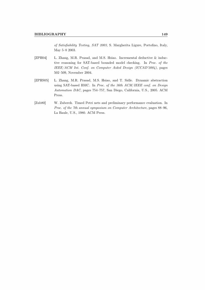
BIBLIOGRAPHY 149
of Satisfiability Testing, SAT 2003, S. Margherita Ligure, Portofino, Italy,May 5–8 2003.
[ZPH04] L. Zhang, M.R. Prasad, and M.S. Hsiao. Incremental deductive & induc-tive reasoning for SAT-based bounded model checking. In Proc. of theIEEE/ACM Int. Conf. on Computer Aided Design (ICCAD’2004), pages502–509, November 2004.
[ZPHS05] L. Zhang, M.R. Prasad, M.S. Hsiao, and T. Sidle. Dynamic abstractionusing SAT-based BMC. In Proc. of the 36th ACM/IEEE conf. on DesignAutomation DAC, pages 754–757, San Diego, California, U.S., 2005. ACMPress.
[Zub80] W. Zuberek. Timed Petri nets and preliminary performance evaluation. InProc. of the 7th annual symposium on Computer Architecture, pages 88–96,La Baule, U.S., 1980. ACM Press.

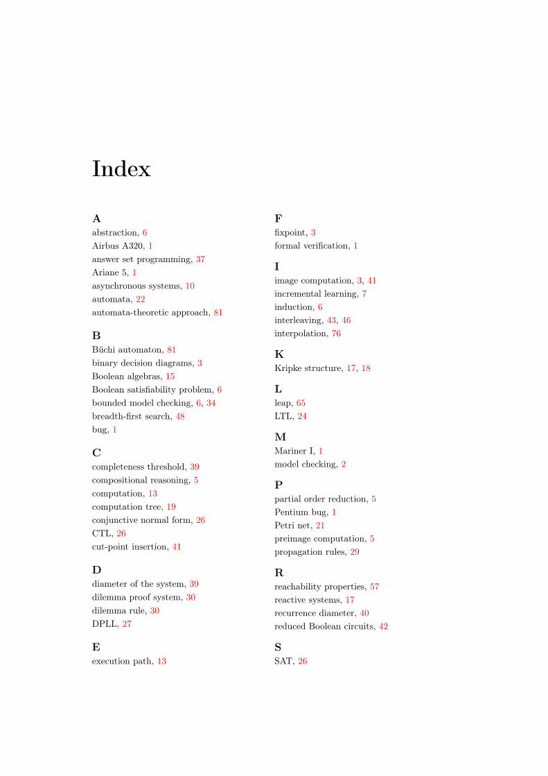
Index
Aabstraction, 6Airbus A320, 1answer set programming, 37Ariane 5, 1asynchronous systems, 10automata, 22automata-theoretic approach, 81
BBüchi automaton, 81binary decision diagrams, 3Boolean algebras, 15Boolean satisfiability problem, 6bounded model checking, 6, 34breadth-first search, 48bug, 1
Ccompleteness threshold, 39compositional reasoning, 5computation, 13computation tree, 19conjunctive normal form, 26CTL, 26cut-point insertion, 41
Ddiameter of the system, 39dilemma proof system, 30dilemma rule, 30DPLL, 27
Eexecution path, 13
Ffixpoint, 3formal verification, 1
Iimage computation, 3, 41incremental learning, 7induction, 6interleaving, 43, 46interpolation, 76
KKripke structure, 17, 18
Lleap, 65LTL, 24
MMariner I, 1model checking, 2
Ppartial order reduction, 5Pentium bug, 1Petri net, 21preimage computation, 5propagation rules, 29
Rreachability properties, 57reactive systems, 17recurrence diameter, 40reduced Boolean circuits, 42
SSAT, 26
152 INDEX
satisfiability modulo theory, 33saturation, 30simulation and testing, 1state, 13state explosion, 5Stålmarck, 28symmetry, 6synchronous, 8synchronous system, 8
Ttemporal logic, 24termination length, 39transition, 13transition systems, 13triplets, 29
Uunbounded model checking, 41unrolling, 34unsatisfiable core, 33, 38