FBTC 2008

Model Checking Biological Oscillators

Ezio Bartocci,1 Flavio Corradini,2 Emanuela Merelli,3

Luca Tesei4

Dipartimento di Matematica e InformaticaUniversity of Camerino

Via Madonna delle Carceri, 9, Camerino (MC), 62032, Italy

Abstract

We define a subclass of timed automata, called oscillator timed automata, suitable to model biologicaloscillators. The semantics of their interactions, parametric w.r.t. a model of synchronization, is introduced.We apply it to the Kuramoto model. Then, we introduce a logic, Kuramoto Synchronization Logic (KSL),and a model checking algorithm in order to verify collective synchronization properties of a population ofcoupled oscillators.

Keywords: Spontaneous synchronization, Kuramoto model, oscillator timed automata, KSL, modelchecking

1 Introduction

Synchronization phenomena in large populations of interacting components arewidely represented in nature and intensively studied as physical, biological, chem-ical, and social systems. In Biology, examples include networks of pacemaker cellsin heart [15], nervous system [8], group of synchronously flashing fireflies [6], just tomention some of those analyzed by Strogatz in his exciting book [16]. Understand-ing a synchronized collective behavior is essential in Systems Biology especially fordeveloping methods to control the dynamics of systems with desired properties [10].

The distributed synchronization of biological systems is commonly modeled us-ing the theory of coupled oscillators proposed by several authors Art Winfree [18],Charles S. Peskin [15] and Yoshiki Kuramoto [11]. In this theory, each member ofthe population is modeled as a phase oscillator running independently at its ownfrequency. The synchronization could be achieved coupling each oscillator to all

1 Email: ezio.bartocci@unicam.it2 Email: flavio.corradini@unicam.it3 Email: emanuela.merelli@unicam.it4 Email: luca.tesei@unicam.it

This paper is electronically published inElectronic Notes in Theoretical Computer Science

URL: www.elsevier.nl/locate/entcs

the others and making them to interact with a certain strength. Whereas, the con-trol is achieved either by introducing artificial oscillators or a new impulse, or bychanging the parameters of individual oscillators. This approach gives rise to anartificial control strategy as it has been proposed by Wang in his recent work [17].In the case of fireflies, an oscillator represents the internal clock dictating whento flash. Upon reception of a pulse from other oscillators, the clock is regulated.Over time, the synchronized behavior emerges, i.e. pulses of different oscillatorsare transmitted simultaneously, and then all fireflies simultaneously flash. Themost successful attempt to model distributed synchronization has been proposedby Yoshiki Kuramoto. The Kuramoto’s model, based on Winfree’s ideas that mu-tual synchronization is a cooperative phenomenon, a temporal analogue of phasetransition encountered in statistical physics, is beautiful and analytically tractablemodel. A wide description of the Kuramoto model can be found in [1].

In this paper, we define a subclass of timed automata, called oscillator timed au-tomata, suitable to model oscillators. Then, we introduce an interaction semanticswhich is parametric w.r.t. a model of synchronization. Subsequently, we instantiateit to the Kuramoto model. The main advantage of our approach is that althoughthe timed automata show different behaviors, w.r.t. their original ones, when inter-acting, we do not need to change their structure. This is obtained by using a globaltime measure, which is the one of the observer, and several internal relative timemeasures, one for each oscillator, which are then re-scaled to the global time.

We also provide a Kuromoto Synchronization Logic (KSL) in order to specifyproperties on synchronization, during a simulation, of Kuramoto based oscillators.Moreover, we propose a model checking algorithm for the logic. We test it byverifying some properties with a prototype simulator and model checker that wehave implemented.

The paper proceeds as follows: Section 2 introduces related works and the Ku-ramoto model. Section 3 recalls timed automata, defines oscillator timed automata,and specifies the interaction semantics. Section 4 introduces the Kuramoto Syn-chronization Logic (KSL) and its model checking algorithm. Section 5 shows anexample of analysis and Section 6 concludes outlining some directions for futurework.

2 Background

2.1 Related work

During these last decades, several mathematical models have been proposed to studythe spontaneous synchronization phenomena in a population of biological coupledoscillators [16]. These models have been inspired by real biological systems, rangingfrom the mutual synchronization of cardiac and circadian pacemaker cells to therhythmically flashing of fireflies and wave propagation in heart, brain, intestine andnervous system. In these systems, mutual synchronization could be performed boththrough episodic impulses and through smooth interactions.

The first case, in which a population of the so called pulse-coupled oscillatorscommunicate by sudden pulse-like interactions - i.e. a neuron that fires - was first

2

studied by Peskin [15], who proposed a model of the mutual synchronization ofsinotrial node pacemaker cells. He worked with identical oscillators and he con-jectured that for any arbitrary conditions, they would all end up firing in unison.He proved this property for N = 2 oscillators and later Mirollo and Strogatz [14]demonstrated that the conjecture holds for all N . Peskin also conjectured that syn-chronization would occur even if the oscillators were not quite identical, but thatproblem remains still open.

For the second case, in which the interactions between oscillators are smooth,a first approach was proposed by Winfree [18] that introduced a model of nearlyidentical, weakly coupled limit-cycle oscillators. Using numerical simulation, hediscovered that for these starting conditions, the system behaves incoherently, witheach oscillator running at its natural frequency. He also found that, as the couplingis increased, the unsynchronized incoherence continues until a certain threshold,when a group of oscillators jump suddenly into synchrony.

Starting from Winfree’s results and assumptions, Kuramoto began working withcollective synchronization phenomena and he proposed a refined model [11,12] pro-viding some analytical tools in order to render the problem more tractable and thesynchronization measurable.

2.2 Kuramoto model

The Kuramoto model of synchronization [13] describes the dynamics of a set of Ninteracting phase oscillators θi with natural frequencies ωi and initial phases θ0

i .The standalone evolution of the i-th oscillator is described by θi(t) = ωit + θ0

i .Intuitively each oscillator i can be visualized as a point moving on a circle of radius1 with angular speed ωi starting at angle θ0

i .When the oscillators interact they tend to adapt themselves, by accelerating or

decelerating, with respect to the phases and the frequencies of the others. Thiscan be viewed as a process of collective synchronization which ends, under certainconditions, in a total synchronous behavior. In the metaphor of the points movingon the circle, when the system becomes synchronized the points move around insync, meaning that the phase differences remain constant. If the oscillators haveidentical natural frequencies, they are also null.

By Kuramoto, the evolution of the interacting i-th oscillator is given by thefollowing equation:

θi = ωi +K

N

N∑j=1

sin(θj − θi), i = 1, · · · , N (1)

where K is the coupling strength depending on the type of interaction. A primarybasic condition to the possibility of synchronization is that the natural frequenciesof the N oscillators are equal or chosen from a lorentzian probability density givenby:

g(ω) =γ

π[γ2 + (ω − ω0)2]where γ is the width and ω0 is the median.

3

In his analysis [13], Kuramoto provided a measure of synchronization by definingthe complex order parameters r and ψ as:

reiψ =1N

N∑j=1

eiθj (2)

where r is the magnitude of the centroid of the points and ψ indicates the averagephase. The radius r represents the phase-coherence of the population of the oscil-lators and it is a convenient measure of the extent of synchronization in the limitN → ∞ and t → ∞. If all oscillators are in sync, r = 1 when all the ωi’s arethe same while r ≈ 1 when the natural frequencies are not identical. On the otherhand, when all oscillators are completely out of phase with respect to each otherthe value of r remains close to 0 most of the time.

In particular Kuramoto found that:

r =

0 K < Kc√

1− (Kc/K) K ≥ Kc

where Kc = 2γ. This means that the oscillators remain completely desynchronizeduntil the coupling strength K exceeds a critical value Kc. After that, the populationsplits into a partially synchronized state consisting of two groups of oscillators: asynchronized group that contributes to the order parameter r, and a desynchronizedgroup whose natural frequencies lie in the tails of the distribution g(ω) and are tooextreme to be entrained. With further increases in K, more and more oscillatorsare recruited into the synchronized group, and r grows accordingly.

Usually, to approximate Equation (1) a suitable discretization is made by fixinga small time interval dt to perform a numerical simulation. See Section 4 for adiscussion on the numerical methods used in our approach.

3 Automata model

In this section we show how oscillators can be modeled by timed automata andhow their interaction semantics can be defined, basing on a synchronization model,without changing the structure of the standalone automata.

3.1 Timed automata

Timed Automata [2] are an established formalism for modeling and verifying real-time systems. They allow strict quantitative real-time constraints to be expressed.This characteristic will be used to model oscillators.

In this section we introduce the basic machinery on timed automata that weneed for our purposes. The idea of clock variables is central in the framework oftimed automata. A clock is a variable that takes values from the set R≥0. The clocksmeasure time as it elapses. All the clocks of a given system advance at the samerate: when increasing, they can be viewed as functions on time whose derivative is

4

equal to 1. Clock variables are ranged over by x, y, z, . . . and we use X ,X ′, . . . todenote sets of clocks. A clock valuation over X is a function assigning a positivenatural number to every clock. The set of valuations of X , denoted by VX , is theset of total functions from X to R≥0. Clock valuations are ranged over by ν, ν ′, . . ..Given ν ∈ VX and δ ∈ R>0, we use ν + δ to denote the valuation that maps eachclock x ∈ X into ν(x) + δ.

Clock variables can be reset during the evolution of the system when certainactions are performed or certain events occur. The reset consists in instantaneouslyset the value of a clock to 0. Immediately after this operation the clock restarts tomeasure time at the same rate as the others. The reset is useful to measure thetime elapsed since the action/event that reset the clock occurred. Given a set X ofclocks, a reset γ is a subset of X . The set of all resets of clocks in X is denotedby ΓX and reset sets are ranged over by γ, γ′, . . . Given a valuation ν ∈ VX and areset γ, we let ν\γ be the valuation that assign the value 0 to every clock in γ andassign ν(x) to every clock x ∈ X − γ.

The timed behavior of the system is expressed using constraints associated to theedges of the automaton. Such constraints depend on the actual values of the clockvariables of the system. Given a set X of clocks, the set ΨX of clock constraints overX are defined by the following grammar: ψ ::= true | false | x #c | x−y # c | ψ∧ψwhere x, y ∈ X , c ∈ N, and # ∈ <,>,≤,≥,=. A satisfaction relation |= is definedsuch that ν |= ψ if the values of the clocks in ν satisfy the constraint ψ in the naturalinterpretation.

Definition 3.1 A Timed Automaton T is a tuple (Q,Σ, E , q0,X , Inv), where: Q isa finite set of locations, Σ is a finite alphabet of symbols, E is a finite set of edges,q0 is the initial state, X is a finite set of clocks, and Inv is a function assigningto every q ∈ Q an invariant, i.e. a clock constraint ψ such that for each clockvaluation ν ∈ VX and for each δ ∈ R>0, ν + δ |= ψ ⇒ ν |= ψ. Constraints havingthis property are called past-closed.

Each edge e ∈ E is a tuple in Q×ΨX × ΓX ×Σ×Q. If e = (q, ψ, γ, a, q′) is anedge, q is the source, q′ is the target, ψ is the constraint, a is the label, and γ is thereset.

We use timed automata with invariants on the states, usually called timed safetyautomata [9], that are the most common in the modeling and verification tools.They incorporate a strong notion of fairness, due to the invariants, which will beuseful for the definition of oscillator timed automata in Section 3.2 and of theinteraction semantics in Section 3.3.

Figure 1(a) shows a sample timed automaton with three states 0, 1, 2. The set ofclocks is x, the alphabet is a, b, 0 is the initial state, and the invariant of state0 is x < 4. There is an edge from state 0 to state 1 with clock constraint x < 4,label a and reset set x.

The semantics of a timed automaton T = (Q,Σ, E , q0,X , Inv), is a labeled tran-sition system S(T ) whose states - ranged over by s, s′, . . . - are pairs (q, ν), whereq ∈ Q is a location of T , and ν ∈ VX is a clock valuation. The transition relationis defined by the following rules:

5

0

1

2 3

4

y<=5

y<=5 y<=5

y<=5

y <5

y>2c

y

cy = 5

y

y=5

yc

y=5

yc

y

c

y=5

y<2

d

yc

y>=0 and

y<=3

(b)

0 1

2

x < 4

x<=4

x<=4

x

x >=1

b

x = 4ax

x<4 a

(a)

Fig. 1. Two oscillator timed automata

T1δ ∈ R>0 ν + δ |= Inv(q)

(q, ν) δ−→(q, ν + δ)T2

(q, ψ, γ, a, q′) ∈ E , ν |= ψ

(q, ν) a−→(q′, ν\γ)

Rule T1 let δ time units to elapse, provided that the invariant of the currentlocation will be satisfied at the reached state. We call the transitions performedusing this rule δ-transitions. Rule T2 describe a transition, labelled by a, of theautomaton which is possible only if the current clock evaluation ν satisfies the clockconstraint of the edge. The effect of the transition is to go in the targe location q′

where the clocks in the reset set γ have been assigned to 0. We call the transitionsperformed using this rule a-transitions.

The initial state of S(T ) is (q0, ν0) where ν0 is the clock valuation assigning 0 toall clocks.

A prefix of a possible behavior of the automaton in Figure 1(a) is rex = (0, [x =0]) 3.4−→(0, [x = 3.4]) a−→(1, [x = 0]) 1.2−→(1, [x = 1.2]) b−→(2, [x = 1.2]) . . .

Let T = (Q,Σ, E , q0,X , Inv) be a timed automaton and let r = s0l0−→ s1

l1−→· · ·be an infinite derivation of S(T ) where s0 = (q0, ν0) is an initial state.

- The time sequence t0 t1 t2 · · · of the times elapsed from state s0 to every statesi = (qi, νi) in r is defined as follows:t−1 = 0

ti+1 = ti +

0 if li ∈ Σ

li otherwise

- The label sequence of r is the sequence of the transitions occurred during r, in-cluding the elapsed times, from the initial state: (l0, t0)(l1, t0) · · ·

- The action sequence of r is the projection of the label sequence of r on the pairs(li, ti) | i ≥ 0, li ∈ Σ

- If a ∈ Σ the a-sequence of r is the projection of the label sequence of r on thepairs (li, ti) | i ≥ 0, li = a

The time sequence of rex is t−1 = 0, t0 = 3.4, t1 = 3.4, t2 = 4.6, t3 = 4.6, . . .

6

The label sequence is (3.4, 3.4)(a, 3.4)(1.2, 4.6)(b, 4.6) · · · The action sequence is(a, 3.4)(b, 4.6) · · · The b-sequence is (b, 4.6) · · ·

3.2 Oscillator timed automata

The following definition characterizes the subclass of timed automata that are suit-able to represent oscillators.

Definition 3.2 A timed automaton T is called oscillator timed automaton on adistinguished action a ∈ Σ with period p ∈ R>0 if and only if all the followingconditions hold:

(i) for all ϑ ∈ R≥0 such that 0 ≤ ϑ < p there exists a prefix of an infinite

derivation r of S(T ) of the form s0l0−→ s1

l1−→· · · ln−1−→ snln−→ sn+1 where all li

(i = 0, . . . , n− 1) are in R>0 (i.e. they are δ-transitions) and ln = a

(ii) every infinite derivation r of S(T ) has a prefix of the form (i)

(iii) every infinite derivation r of S(T ) has an infinite a-sequence of the form(a, ϑ)(a, 1 · p+ ϑ)(a, 2 · p+ ϑ)(a, 3 · p+ ϑ) · · · for some delay ϑ

(iv) every finite derivation of S(T ) is a prefix of an infinite derivation r of S(T )

This definition constrains an oscillator timed automaton to have an initial statefrom which the oscillation can start with every delay (i), to always perform thedistinguished action as the first action (ii), to regularly repeat the distinguishedaction every period from the first action on (iii), and to not have dying paths (iv),that is paths ending in a state where time can not proceed.

Such a behavior is a convenient representation of an oscillator with its own initialphase θ0 (0 ≤ θ0 < 2π), which we represent here as a time delay ϑ instead of anangle, and its own frequency ω, which we represent here as a period p. They arerelated as follows: ω = 2π

p and θ0 = 2πp ϑ.

Figure 1(a) is an oscillator timed automaton on the distinguished action a withperiod 4. In Figure 1(b) we show a slightly more complex automaton which is anoscillator timed automaton on the distinguished action c with period 5. Note thatthere is non-determinism on the choice of the initial non-δ-transition. Moreover,there may be both an infinite self-loop on state 1 and a cycle between states 3and 4 that eventually could end in the loop of state 1. In general, oscillator timedautomata can be very complex automata performing several actions and involvingcycles other than the one we focus on. The choice of the distinguished actionidentifies the particular observation with which an external observer recognizes theoscillating behavior.

3.3 Interacting oscillator timed automata

We want to describe the interaction among several oscillator timed automata. Thedefinition we give here is parametric with respect to the model of synchronization.After the parametric definition we introduce the particular instance that uses theKuramoto model.

Let T1, . . . , TN be oscillator timed automata on distinguished actions a1, . . . , aN

7

with periods p1, . . . , pN . We suppose we are given, randomly determined or specif-ically chosen, N initial delays ϑ1, . . . , ϑN .

At every instant of the interaction process we need to keep track of the currentposition of each oscillator in its standalone cycle. To do this we define a simpletransformation: we add a new clock xi to every Ti and, to guarantee a correctmeasure, we modify each Ti in such a way that xi is reset whenever the distin-guished action ai is performed by Ti. This can be easily done by replacing eachedge (q, ψ, γ, ai, q′) of Ti by (q, ψ, γ ∪ xi, ai, q′).

The previous transformation ensures that, after a proper initialization, xi mea-sures, at every point of the evolution of S(Ti), the time elapsed since the lastoccurrence of ai. By the assumption that Ti is an oscillator timed automaton, wecan also state that pi minus the value of xi measures the remaining time to the nextoccurrence of ai. The initialization process is described below.

3.3.1 Steps of activityIn order to describe the interaction semantics we need to define the steps of activityof a single automaton.

Let T = (Q,Σ, E , q0,X , Inv) be a timed automaton. Given ∆ ∈ R>0 we definea transition relation `−→

∆between two states of S(T ). We say that (q, ν) `−→

∆(q′, ν ′)

if and only if there exists a finite derivation d of S(T ) of the form (q, ν) =

(q0, ν0) l0−→(q1, ν1) l0−→· · · ln−1−→(qn, νn) = (q′, ν ′) such that:

• ` is the string l0l1 · · · ln−1

• ∆ is the sum of the times elapsed during d, i.e. ∆ =∑n−1

i=0,li∈R>0 li

The time sequence of d is defined as the time sequence of r in Section 3.1,starting from state (q, ν) and ending on state (q′, ν ′). The label sequence, actionsequence and a-sequence of d are defined in the same way. Note that in this casethe sequences are all finite. Moreover, given a step (q, ν) `−→

∆(q′, ν ′), we define a

function A such that A(`) gives the action sequence of the derivation d associatedto the step.

The steps of activity allow us to group a sequence of transitions of S(T ) into asingle transition `−→

∆. We can decide the amount of time (∆) of our observation (`)

of the automaton behavior. Note that a step of activity is always possible only ifthe automaton has not dying paths. Since we use this transition relation only withoscillator timed automata, this is guaranteed by Definition 3.2:

Proposition 3.3 Let T be an oscillator timed automaton and let(q0, ν0) l0−→· · · ln−→(q, ν) be a finite derivation of S(T ). Then, given ∆ ∈ R>0, it isalways possible to perform a step of activity (q, ν) `−→

∆(q′, ν ′).

Proof. By property (iv) of oscillator timed automata expressed in Definition 3.2.2

8

3.3.2 InitializationThe initialization step of the interaction must ensure that we start each transitionsystem S(Ti) in a state with complete information about the delay and, thus, aboutthe values of xi and the other clocks. To achieve this requirement we need to performa preliminary collective derivation of all S(Ti). Before describing the procedure weneed to introduce the following proposition.

Proposition 3.4 Let T = (Q,Σ, E , q0,X , Inv) be an oscillator timed automatonon the distinguished action a with period p. For all delays 0 ≤ ϑ < p, there exists

an edge (q0, ψ, γ, a, q′) ∈ E and a prefix d = s0

l0−→ s1l1−→· · · ln−1−→ sn

ln−→ sn+1 of aninfinite derivation r of S(T ) such that:

• all li, i = 0, . . . , n− 1, are in R>0,∑n−1

i=1 li = ϑ and ln = a

• sn = (q0, ν0 + ϑ) and sn+1 = (q′, (ν0 + ϑ)/γ)

Proof. The properties follow easily by Definition 3.2 and by the semantics of atimed automaton. 2

The previous Proposition implies that we can effectively determine a state sn+1

of S(T ) from which the actual interaction of the automaton with the others canstart.

Let B1, B2, . . . , BK , K ≤ N , be a sequence of non-empty sets partitioning1, . . . , N such that for all k, k = 1, 2, . . . ,K − 1, if i ∈ Bk and j ∈ Bk+1 thenϑi < ϑj ; i.e. every Bk contains the indexes of the automata with equal values ofinitial delay and the sequence arranges the indexes of automata in such a way thattheir initial delays are in strict ascending order.

The preliminary collective derivation is as follows. It is straightforward, butrequires a lot of details: for the sake of brevity we only give a brief informal de-scription.

We consider the initial states s10, s

20, . . . , s

N0 of each S(Ti), where every Ti has been

transformed inserting the new clock and modifying the edges as specified above.The process is a sequence of K steps. At the first step every S(Ti) performs zero

or more δ-transitions in order to reach a state of the form (q0, ν0 +ϑ) where ϑ is thedelay of the first group of oscillators whose indexes are in B1. Then, the automata inthis group perform a further single a-transition (where a is the distinguished action)to reach a state of the form (q′, (ν0 +ϑ)/γ), as guaranteed by Proposition 3.4. Fromnow on every automaton of this group is considered “activated” and continues witha sequence of transitions of the form `−→

∆where ∆ is given by the times specified in

the subsequent steps.At the i-th step the time that has to pass is ϑ = ϑk − ϑj , where j ∈ Bi−1 and

k ∈ Bi. The previously “activated” automata perform a transition `−→ϑ

, while all

the others perform δ-transitions for a total of ϑ time units. Then, the automatawhose indexes are in Bi becomes “activated” performing their first a-transition (adistinguished). Again, this possibility is guaranteed by Proposition 3.4.

At the end of this process we group the N reached states into a tuple〈s1

0, s20, . . . , s

N0 〉 which is the initial configuration of the interaction semantics. Note

that, during the process, the early “activated” automata could have performed other

9

a-transitions, even distinguished ones. This does not influence the subsequent in-teractions, because there have not been perturbations due to the synchronizationfunction. The important fact to remark is that the states of the starting tuple allhave pertinent values for the clocks xi and represent running oscillators with thechosen delays and periods.

3.3.3 Interaction semanticsNow we can introduce the behavior of N oscillator timed automata running inparallel and interacting using a generic discretized model, which is represented byan interaction function I.

The main advantage of the interaction semantics is that it maintains the struc-ture of the automata Ti’s, though it defines a perturbed behavior of them due to theinteraction. This is achieved by using a global time, which is the time measure of theobserver, together with N different relative times, which are the internal time mea-sures of each oscillator timed automata involved. This means that if, according tothe interaction, Ti has to decelerate and Tj has to accelerate during the current sliceof global time dt, then Ti performs a step of activity whose duration is shorter thandt, while Tj performs a longer one. The acceleration and deceleration is determinedby the interaction function I of the particular chosen model of synchronization. Theglobal observer detects perturbed behaviors because the timestamps of the actionsperformed by each interacting Ti are re-scaled to the magnitude of the global timeslice dt.

Now we can introduce a transition relation, which we call progress relation,between configurations, i.e. tuples 〈s1, s2, . . . , sN 〉 where each si is a state of S(Ti).The rule defining the relation is the following:

∀i = 1, 2, . . . N ∆i = I(i, dt, s1, s2, . . . , sN ) si`i−→∆i

s′i λi = SC(A(`i),∆i, dt)

〈s1, s2, . . . , sN 〉λ1,λ2,...,λN

−−−−−−−→dt

〈s′1, s′2, . . . , s′N 〉

where the re-scaling function SC is defined as follows:

SC((a0, t0)(a1, t1) · · · (ak, tk),∆, dt) = (a0,t0∆· dt)(a1,

t1∆· dt) · · · (ak,

tk∆· dt)

The behavior of the interacting oscillator timed automata T1, T2, . . . , TN is thendefined as an infinite derivation:

ρ = 〈s10, s

20, . . . , s

N0 〉

λ10,λ

20,...,λ

N0−−−−−−−→

dt〈s1

1, s21, . . . , s

N1 〉

λ11,λ

21,...,λ

N1−−−−−−−→

dt· · ·

To construct the trace associated to ρ, we need a function Ω that merges thescaled action sequences λ1, λ2, . . . , λN of every step of progress into one action se-quence in which the timestamps of each action are in ascending order. Moreover weneed a function T (τ, (a0, t0)(a1, t1) · · · (ak, tk)) = (a0, t0+τ)(a1, t1+τ) · · · (ak, tk+τ)that adds a given amount of time τ to the timestamps of an action sequence.

Definition 3.5 Given N interacting oscillator timed automata T1, . . . , TN ,

10

the trace associated to a derivation ρ = 〈s10, s

20, . . . , s

N0 〉

λ10,λ

20,...,λ

N0−−−−−−−→

dt

〈s11, s

21, . . . , s

N1 〉

λ11,λ

21,...,λ

N1−−−−−−−→

dt〈s1

2, s22, . . . , s

N2 〉

λ12,λ

22,...,λ

N2−−−−−−−→

dt· · · is the following action

sequence:

Ω(λ10, λ

20, . . . , λ

N0 ) T (1 · dt,Ω(λ1

1, λ21, . . . , λ

N1 )) T (2 · dt,Ω(λ1

2, λ22, . . . , λ

N2 )) · · ·

The observable behaviors of the interacting oscillator timed automata are all possibletraces.

Note that traces contain all the actions performed by all the interacting au-tomata. Moreover, the timestamp of each action is the one perceived by the globalobserver, which can therefore detect the perturbations, due to interaction, on theoriginal standalone behaviors. Projecting a trace on distinguished actions onlyallows to observe the synchronization process if, eventually, all the distinguishedactions occur at the same times.

3.3.4 Kuramoto interactionIn this section we instantiate the interaction semantics given above to the discretizedKuramoto model of synchronization introduced in Section 2.2.

In the automata model we use periods instead of natural frequencies and initialdelays instead of initial phases. Since the Kuramoto model is defined in terms ofangular frequency and angular acceleration, we need to do a simple transformationto express the acceleration K

N

∑Nj=1 sin(θj − θi) of the i-th oscillator in terms of

shorter or longer duration ∆i of the step of activity of Ti at each progress of lengthdt. This is what the function I does, which is described in the following.

First, note that each configuration 〈s1, s2, . . . , sN 〉 is a snapshot of the situationof each oscillator at a given point of time t. This situation can be depicted in acircle of radius 1 associating to each automaton Ti, modulo 2πh for some h ∈ N,the angle θi(t) = ui

pi· 2π, where ui is the time elapsed since the last occurrence of

the distinguished action ai. By the transformation described at the beginning ofSection 3.3, we know that ui is precisely the value of the clock xi that can be derivedfrom si = (q, ν) as ν(xi). Note that this is true also in the starting configuration(for which we consider t = 0), as we showed in Section 3.3.2.

Using this transformation we can calculate the quantity

αi =K

N

N∑j=1

sin(θj(t)− θi(t))

for each automaton Ti. Then, according to the discretization of the Kuramoto model(see Section 2.2), during the time slice dt the i-th oscillator has to move forward,in the circle representation, of an angle (ωi + αi)dt, where ωi = 2π

piis its natural

frequency. The time ∆i the automaton Ti has to consume to do this is such that(ωi+αi)dt = ωi∆i. Thus, ∆i = dt+ αidt

ωi, which is the value of I(i, dt, s1, s2, . . . , sN ).

11

4 Logic for biological oscillators

In this section, we introduce a logic, Kuramoto Synchronization Logic (KSL), inorder to specify and detect collective synchronization properties in a populationof oscillator timed automata. We provide the syntax, the semantics and a modelchecking algorithm for KSL. This logic has the same main temporal and logicaloperators as Linear Temporal Logic (LTL). However, while LTL use a finite stateautomaton, the Kripke structure, as a model, KSL use an uncountable state model.In KSL, atomic propositions are given in terms of equalities or inequalities aboutlinear combinations of state variables. This form allows us to easily describe someuseful properties about synchronization. We add a special operator D., inspiredby the freeze quantification of [3], to store state variables in a certain step of thesimulation that could be compared with the state variables of a successive step.Moreover, we use a bounded version of the until operator U adding to it a constrainton the maximum time interval to be considered.

4.1 Discrete time Kuramoto model

Our system model is a discrete time version of the Kuramoto model (see Equa-tion (1)) which can be represented by a tuple M = (Ω,Θ,D,D(∗),K, r), whereΩ = ω1, · · · , ωn is the vector of frequencies of the oscillator timed automata,Θ = θ1, · · · , θn is the vector of the initial phases, D = d1, · · · , dn is the vectorof the remaining times to accomplish the distinguished actions, D(∗) are the set ofvectors of the stored remaining times during simulation, K ∈ R is the interactionconstant between the oscillators automata, and r is the phase coherence calculatedat current time as in Equation (2). We overload the definition of θi, di and r withthe functions θi : N → R, di : N → R and r : N → R that map the discrete time tto the value of synchronization phases, remaining times and phase coherence.

The relations among synchronization phases and remaining times are given bythe following equations:

θi(t+ dt) = θi(t) + (ωi +n∑j=1

K

nsin(θi(t)− θj(t))dt (3)

di(t+ dt) =(2qπ − θi(t+ dt))

ωisuch that q = min(z ∈ N : 2zπ ≤ θi(t+ dt))

If we consider dt as the time unit in the discretization of time we can rewriteEquation (3) as follows:

θi(t) = θi(0) +t−1∑l=0

ωi +n∑j=1

K

nsin(θi(l)− θj(l))

dt (4)

where θi(0) is the synchronization phase at the beginning of the simulation.Although Equation (3) and (4) are very intuitive to understand and simple to be

calculated, they need a very small dt to provide a good approximation, increasingdramatically the number of simulation steps. Consequently, in the simulator we

12

implemented, we used the Runge-Kutta 4th order method [7] to obtain the bestcompromise between the approximation and the speed of computation.

4.2 Syntax and semantics of Kuramoto Synchronization Logic

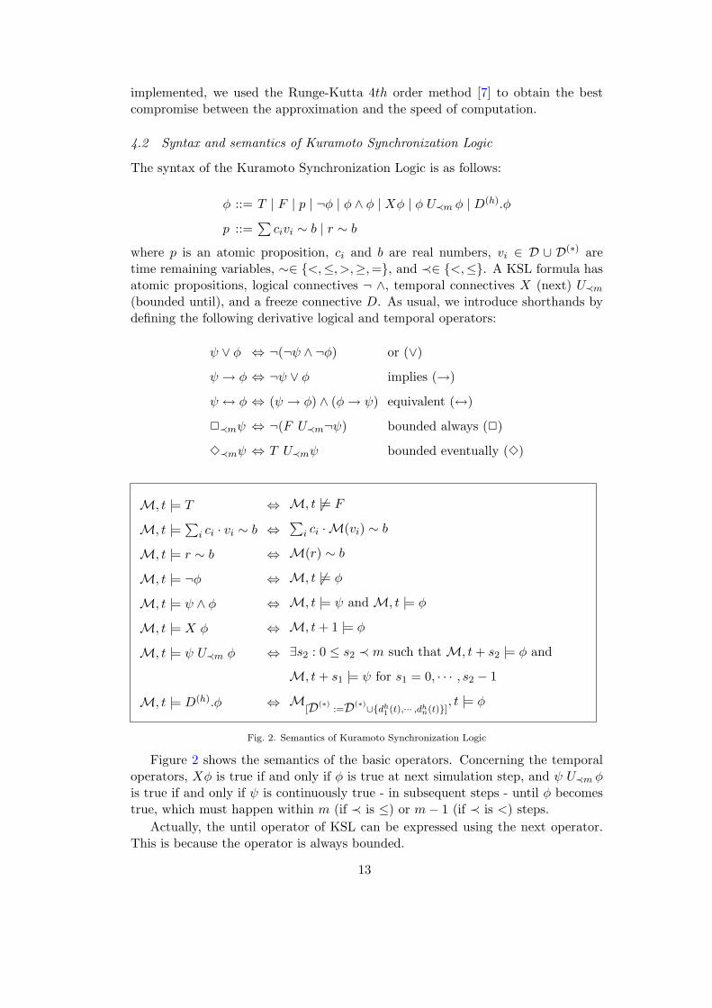
The syntax of the Kuramoto Synchronization Logic is as follows:

φ ::= T | F | p | ¬φ | φ ∧ φ | Xφ | φ U≺m φ | D(h).φ

p ::=∑civi ∼ b | r ∼ b

where p is an atomic proposition, ci and b are real numbers, vi ∈ D ∪ D(∗) aretime remaining variables, ∼∈ <,≤, >,≥,=, and ≺∈ <,≤. A KSL formula hasatomic propositions, logical connectives ¬ ∧, temporal connectives X (next) U≺m(bounded until), and a freeze connective D. As usual, we introduce shorthands bydefining the following derivative logical and temporal operators:

ψ ∨ φ

ψ → φ

ψ ↔ φ

2≺mψ

3≺mψ

⇔

⇔

⇔

⇔

⇔

¬(¬ψ ∧ ¬φ)

¬ψ ∨ φ

(ψ → φ) ∧ (φ→ ψ)

¬(F U≺m¬ψ)

T U≺mψ

or (∨)

implies (→)

equivalent (↔)

bounded always (2)

bounded eventually (3)

M, t |= T

M, t |=∑

i ci · vi ∼ b

M, t |= r ∼ b

M, t |= ¬φ

M, t |= ψ ∧ φ

M, t |= X φ

M, t |= ψ U≺m φ

M, t |= D(h).φ

⇔

⇔

⇔

⇔

⇔

⇔

⇔

⇔

M, t 6|= F∑i ci · M(vi) ∼ b

M(r) ∼ b

M, t 6|= φ

M, t |= ψ and M, t |= φ

M, t+ 1 |= φ

∃s2 : 0 ≤ s2 ≺ m such that M, t+ s2 |= φ and

M, t+ s1 |= ψ for s1 = 0, · · · , s2 − 1

M[D(∗)

:=D(∗)∪dh1 (t),··· ,dh

n(t)], t |= φ

Fig. 2. Semantics of Kuramoto Synchronization Logic

Figure 2 shows the semantics of the basic operators. Concerning the temporaloperators, Xφ is true if and only if φ is true at next simulation step, and ψ U≺m φ

is true if and only if ψ is continuously true - in subsequent steps - until φ becomestrue, which must happen within m (if ≺ is ≤) or m− 1 (if ≺ is <) steps.

Actually, the until operator of KSL can be expressed using the next operator.This is because the operator is always bounded.

13

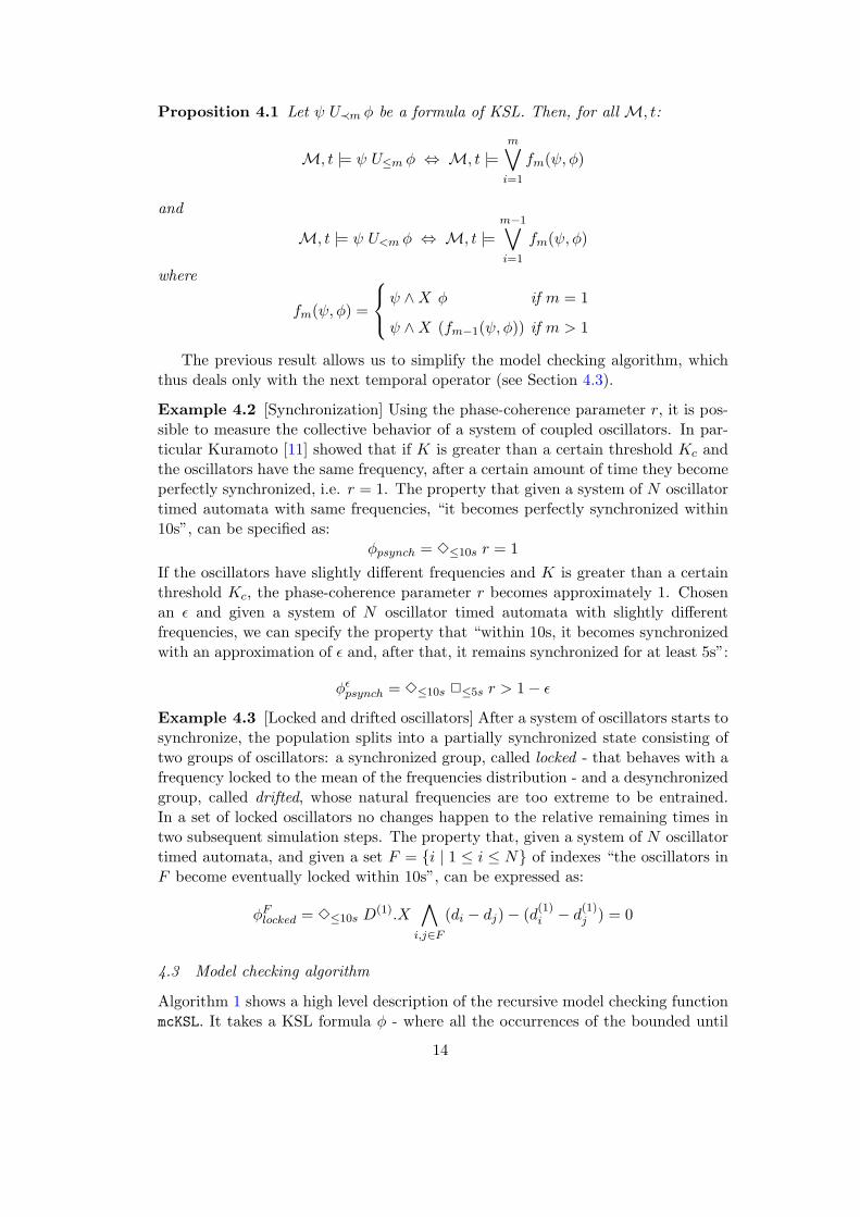
Proposition 4.1 Let ψ U≺m φ be a formula of KSL. Then, for all M, t:

M, t |= ψ U≤m φ ⇔ M, t |=m∨i=1

fm(ψ, φ)

and

M, t |= ψ U<m φ ⇔ M, t |=m−1∨i=1

fm(ψ, φ)

where

fm(ψ, φ) =

ψ ∧X φ if m = 1

ψ ∧X (fm−1(ψ, φ)) if m > 1

The previous result allows us to simplify the model checking algorithm, whichthus deals only with the next temporal operator (see Section 4.3).

Example 4.2 [Synchronization] Using the phase-coherence parameter r, it is pos-sible to measure the collective behavior of a system of coupled oscillators. In par-ticular Kuramoto [11] showed that if K is greater than a certain threshold Kc andthe oscillators have the same frequency, after a certain amount of time they becomeperfectly synchronized, i.e. r = 1. The property that given a system of N oscillatortimed automata with same frequencies, “it becomes perfectly synchronized within10s”, can be specified as:

φpsynch = 3≤10s r = 1If the oscillators have slightly different frequencies and K is greater than a certainthreshold Kc, the phase-coherence parameter r becomes approximately 1. Chosenan ε and given a system of N oscillator timed automata with slightly differentfrequencies, we can specify the property that “within 10s, it becomes synchronizedwith an approximation of ε and, after that, it remains synchronized for at least 5s”:

φεpsynch = 3≤10s 2≤5s r > 1− ε

Example 4.3 [Locked and drifted oscillators] After a system of oscillators starts tosynchronize, the population splits into a partially synchronized state consisting oftwo groups of oscillators: a synchronized group, called locked - that behaves with afrequency locked to the mean of the frequencies distribution - and a desynchronizedgroup, called drifted, whose natural frequencies are too extreme to be entrained.In a set of locked oscillators no changes happen to the relative remaining times intwo subsequent simulation steps. The property that, given a system of N oscillatortimed automata, and given a set F = i | 1 ≤ i ≤ N of indexes “the oscillators inF become eventually locked within 10s”, can be expressed as:

φFlocked = 3≤10s D(1).X

∧i,j∈F

(di − dj)− (d(1)i − d

(1)j ) = 0

4.3 Model checking algorithm

Algorithm 1 shows a high level description of the recursive model checking functionmcKSL. It takes a KSL formula φ - where all the occurrences of the bounded until

14

function mcKSL(φ,M, t,diagTrace). Returns (true, ) or (false, a diagnostic trace)

select casecase φ = T

return (True, )end casecase isAtomic(φ)

return checkAtomicProp(φ,M, t,diagTrace)end casecase φ = ¬φ1

return notDiag(mcKSL(φ1,M, t,diagTrace), φ1,M, t,diagTrace)end casecase φ = φ1 ∧ φ2

return mergeAnd(mcKSL(φ1,M, t,diagTrace),mcKSL(φ2,M, t,diagTrace))

end casecase φ = X φ1

diagTrace← append(diagTrace, φ,M, t)M← nextStep(M)return mcKSL (φ1,M, t+ 1,diagTrace)

end casecase φ = D(h). φ1

diagTrace← append(diagTrace, φ,M, t)M← addVariables(M, h)return mcKSL (φ1,M, t,diagTrace)

end caseend select

end function

Algorithm 1. mcKSL Algorithm

operator have been translated as shown in Proposition 4.1 - a tupleM, a discretizedtime (initially 0), and a dignostic trace (initially empty). The function evaluatesthe formula φ over M and gives a counterexample (a diagnostic trace) wheneverthe formula is false. The complexity of mcKSL is linear with respect to the lengthof the formula, O(|φ|). The addVariables function allows to store the current statevariables di : i = 1, · · · , N in M, when a freeze connective is met during theparsing. For each X connective in the formula, a nextStep function is called inorder to calculate the evolution of the system using the discrete time Kuramotomodel described in Equation (3). The functions notDiag and mergeAnd simplymanage the returning of a correct counterexample, given the results of the recursivecalls.

5 Reasoning on synchronization

In this section we briefly report an example of analysis performed by a prototypeimplementation of our model checker. A demo of the simulator is available at [5].

15

Fig. 3. Initial conditions of the analysis

Fig. 4. Verification of properties after 10 seconds

We generated a system of 40 oscillators by choosing randomly the initial phase syn-chronizations in the range (0, 2π) and frequencies using a Cauchy random variablein the range (0, 1). Figure 3 shows the distribution of frequencies and of phases ofeach oscillator. We set the coupling strength k = 1.0 and we check the φlockedF withF = 1, · · · , 40 and φpsynch with ε = 0.3. Figure 4 shows the result of the modelchecking after 10 seconds.

16

6 Conclusion and future work

In this paper we have defined a subclass of timed automata, oscillator timed au-tomata, suitable to model biological oscillators. We have specified an interactionsemantics, parametric w.r.t. a model of synchronization, and we have instantiatedit to the Kuramoto model. The main advantage of the semantic definition is that itdoes not require changing the structure of the automata modeling the standalone os-cillators. We have also introduced a logic, Kuramoto Synchronization Logic (KSL),in order to specify and detect collective synchronization properties in a populationof oscillators timed automata. A model checking algorithm has been presented andan example of analysis has been showed.

The main future directions of our work are: 1) extend our logic with controloperators that allow us to infer how to influence a set of oscillators by addingartificial oscillators, which we can control, in order to satisfy a desired property. 2)Use hybrid automata, instead of timed automata, to model oscillators and to definethe interaction semantics. 3) Fully implement a model checker and simulator forKSL. A prototype is available at [5]. 4) A long term objective: apply the modelchecking of the extended logic, together with detection techniques already partiallyavailable, to control fibrillation in cardiac cells networks (for more details of thisline of research see [4]).

Acknowledgement

Research partially supported by the Italian FIRB-MIUR LITBIO: Laboratory forInterdisciplinary Technologies in Bioinformatics.

References

[1] Acebron, J., L. Bonilla, C. Perez Vicente, F. Ritort and R. Spigler, The Kuramoto model: A simpleparadigm for synchronization phenomena, Rev Mod Phys 77 (2005), pp. 137–185.

[2] Alur, R. and D. L. Dill, A theory of timed automata, Theoretical Computer Science 126 (1994), pp. 183–235.

[3] Alur, R. and T. A. Henzinger, A really temporal logic, Journal of the ACM 41 (2004), pp. 181–203.

[4] Bartocci, E., F. Corradini, R. Grosu, E. Merelli, S. Smolka and O. Riganelli, “StonyCam: a FormalFramework for Modeling, Analyzing and Regulating Cardiac Myocytes,” Lecture Notes in ComputerScience, Springer-Verlag, 2008 pp. 493–502.

[5] Bartocci, E., F. Corradini, E. Merelli and L. Tesei, Prototype of the KSL model checker and simulator.URL http://cosy.cs.unicam.it/kuramoto/

[6] Buck, J., Synchronous rhythmic flashing of fireflies II, The Quarterly Review of Biology 63 (1988),pp. 265–289.

[7] Butcher, J. C., “Numerical methods for ordinary differential equations,” John Wiley and Sons, 2003.

[8] Dye, J., Ionic and synaptic mechanisms underlying a brainstem oscillator: An in vitro study of thepacemaker nucleus of apteronotus, Journal of Comparative Physiology 168 (1991), pp. 521—-532.

[9] Henzinger, T. A., X. Nicollin, J. Sifakis and S. Yovine, Symbolic model checking for real-time systems,Information and Computation 111 (1994), pp. 193–244.

[10] Kitano, H., “Foundations of Systems Biology,” MIT Press, 2002.

[11] Kuramoto, Y., Phase dynamics of weakly unstable periodic structures: Condensed matter and statisticalphysics, Progress of theoretical physics 71 (1984), pp. 1182–1196.

17

[12] Kuramoto, Y., Collective synchronization of pulse-coupled oscillators and excitable units, Physica D50 (1991), pp. 15–30.

[13] Kuramoto, Y., “Chemical Oscillations, Waves, and Turbulence,” Springer-Verlag, 2003.

[14] Mirollo, R. E. and S. H. Strogatz, Synchronization of pulse-coupled biological oscillators, SIAM Journalof Applied Mathematics 50 (1990), pp. 1645–1662.

[15] Peskin, C. S., “Mathematical Aspects of Heart Physiology,” Courant Institute of Mathematical Sciences,New York University, New York, 1975.

[16] Strogatz, S. H., “SYNC, the emerging science of spontaneous order,” Hyperion, 2004.

[17] Wang, R., L. Chen and K. Aihara, Synchronizing a multicellular system by external input: an artificialcontrol strategy, Bioinformatics 22 (2006), pp. 1775–1781.

[18] Winfree, A. T., Biological rhythms and the behavior of populations of coupled oscillators, Journal ofTheoretical Biology 16 (1967), pp. 15 – 42.

18