Nonstandard Bifurcations in Oscillators with Multiple Discontinuity Boundaries

Nonlinear Dynamics 35: 41–59, 2004.© 2004 Kluwer Academic Publishers. Printed in the Netherlands.

Nonstandard Bifurcations in Oscillators with MultipleDiscontinuity Boundaries

PAOLO CASINI and FABRIZIO VESTRONI∗Dipartimento di Ingegneria Strutturale e Geotecnica, Facoltà di Ingegneria, Università degli Studidi Roma ‘La Sapienza’, via Eudossiana 18, I-00184 Rome, Italy; ∗Author for correspondence(e-mail: [email protected])

(Received: 17 March 2003; accepted: 16 October 2003)

Abstract. The model of a double-belt friction oscillator is proposed, which exhibits multiple discontinuity bound-aries in the phase space. The system consists of a simple oscillator dragged by two different rough supports movingwith constant driving velocities and subjected to an elastic restoring force and viscous damping. Self-sustainedoscillations have been observed to occur, with nonstandard attracting properties. By considering the problem froma nonsmooth dynamical systems perspective, the evolution of steady state attractors as the velocities of the beltsare varied is described. The nonsmoothness sets of the system at hand and, in particular, the presence of multiplediscontinuity boundaries, lead to nonstandard bifurcations which are studied here by means of analytical andnumerical tools.

Keywords: discontinuous boundaries, friction oscillators, nonsmooth dynamics, nonstandard bifurcations

1. Introduction

In recent years, much research effort in science and engineering has focussed on nonsmoothdynamical systems [1–11]. These systems are described by sets of piecewise smooth ordinarydifferential equations which are smooth in regions of phase space: smoothness is lost as tra-jectories cross the boundaries between adjacent regions (discontinuity boundaries). Thus, thephase space of a general nonsmooth dynamical system can be divided into countably manyregions, in each region the system having a different smooth functional form of the vectorfield. Hence, these systems are often referred to as piecewise smooth dynamical systems(PSS). As will be explained later in more detail, across a discontinuity boundary PSS arecalled continuous if the system vector field is the same in the adjacent regions separated bythe boundary, whereas its Jacobian changes [10]; they are called discontinuous, Filippov orswitched systems, if the system vector field changes passing from a region to the adjacentone [1, 6]; finally, PSS are called hybrid, according to the definition given in [3], if across aboundary the system vector state is discontinuous.

Among the most popular examples of continuous PSS there are mechanical systems char-acterized by discontinuous compliance [3]: namely, oscillators colliding with a deformablestop, block assemblies connected by no-tension springs, beams with breathing cracks. Stick-slip mechanical systems characterized by friction contacts are a widely studied example of Fil-ippov systems [2, 4, 5, 12]. Finally, hybrid systems include important applications concerningmechanical systems characterized by impacts as rocking blocks and oscillators colliding withrigid stops [9, 11, 13–16]. The above mentioned examples are taken from the mechanical field,however interesting problems concerning PSS can be formulated also in: switching circuit

42 P. Casini and F. Vestroni

in power electronics, physiological models, internal combustion engine, walking machines,control of renewable resources.

Despite their widespread use, there is no effective systematic theory of such systems yet.In particular, as the systems parameters are varied, novel transitions have been observed ina number of real-word systems which cannot been explained in terms of well-known stan-dard bifurcations for smooth systems. To explain the increasing experimental and numericalevidence of their occurrence, a number of different definitions and notations to describe phe-nomena which are sometimes very similar to each other have been proposed. Recent papers[6, 8, 10] aimed to show how some of the existing results can be organized in a coherent wayin order to set the foundations of a consistent theory of bifurcation in continuous and Filippovsystems; however understanding bifurcations in piecewise smooth systems is still the subjectof much ongoing research.

PSS can exhibit most of the bifurcations also exhibited by smooth systems; in additionthey also show some novel transitions which are unique to PSS. In the Russian literature thesenovel transitions were given the collective name of C-bifurcations: they include interactionsof fixed points and limit cycles with the system discontinuity boundaries and their definition[7, 8, 10] does not necessarily imply the onset on a nontopologically equivalent phase portraitat the bifurcation point. Therefore in the following the term C-bifurcation or, more gener-ally, nonstandard bifurcation will be used to indicate a nonstandard transition in PSS as, forinstance, the grazing bifurcation or the sliding bifurcation [8].

In this paper, a model of double-belt friction oscillator (DBO) is proposed in which mul-tiple discontinuity boundaries exist: they are caused by the presence of friction which ismodelled by a velocity dependent friction law. This model allows a simple representationof engineering applications with multiple nonsmooth characteristics as for instance frictionwheels or slipping mechanisms in multi-block structures. The paper aims to describe the evo-lution of steady state attractors as some system parameters are varied, precisely the velocitiesof the belts. Attention is paid to the transitions which involve interactions between systemtrajectories and phase space discontinuity boundaries: these transitions are unique in theirnature since they depend on the nonsmoothness sets of the system at hand and, in particular,on the presence of multiple discontinuity boundaries. The results obtained for this particularcase study could help to build a complete bifurcation theory in nonsmooth systems.

2. System Modelling

2.1. BACKGROUND

Piecewise smooth systems are described by a finite set of ordinary differential equations

x = fi(x; p), x ∈ Di ⊂ Rn, (1)

where x ∈ Rn is the state vector, p ∈ Rm is a parameter vector, Di, i = 1, 2, . . . , N , areclosed and connected regions of phase space, fi : Rn+m → Rn are smooth functions definedin Di . The boundaries

∑ij between adjacent regions are (n−1)-dimensional manifolds, called

discontinuity boundaries, switching manifolds or nonsmoothness sets.As it has been mentioned above, across the boundaries

∑ij , PSS are characterized by

different discontinuities which can be collected into four classes:

1. continuous vector field but discontinuous Jacobian, i.e. fi = fj but ∇xfi �= ∇xfj ;

Nonstandard Bifurcations in Oscillators with Multiple Discontinuity Boundaries 43

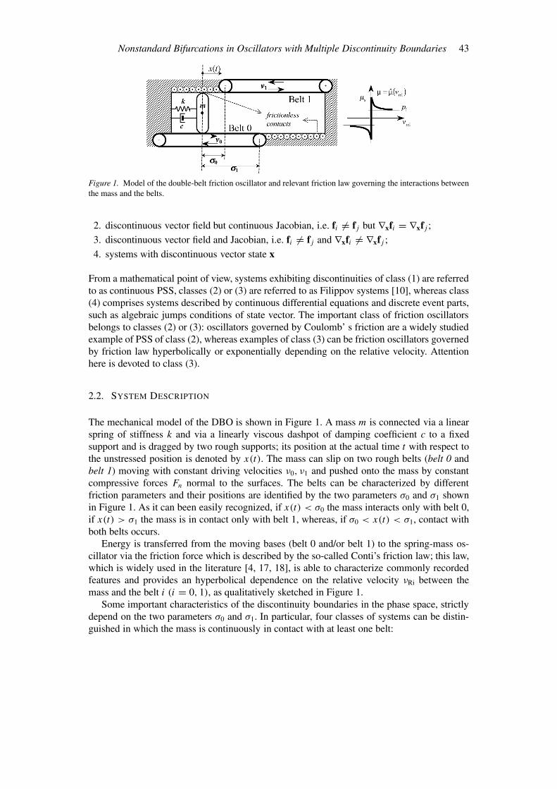
Figure 1. Model of the double-belt friction oscillator and relevant friction law governing the interactions betweenthe mass and the belts.

2. discontinuous vector field but continuous Jacobian, i.e. fi �= fj but ∇xfi = ∇xfj ;

3. discontinuous vector field and Jacobian, i.e. fi �= fj and ∇xfi �= ∇xfj ;

4. systems with discontinuous vector state x

From a mathematical point of view, systems exhibiting discontinuities of class (1) are referredto as continuous PSS, classes (2) or (3) are referred to as Filippov systems [10], whereas class(4) comprises systems described by continuous differential equations and discrete event parts,such as algebraic jumps conditions of state vector. The important class of friction oscillatorsbelongs to classes (2) or (3): oscillators governed by Coulomb’ s friction are a widely studiedexample of PSS of class (2), whereas examples of class (3) can be friction oscillators governedby friction law hyperbolically or exponentially depending on the relative velocity. Attentionhere is devoted to class (3).

2.2. SYSTEM DESCRIPTION

The mechanical model of the DBO is shown in Figure 1. A mass m is connected via a linearspring of stiffness k and via a linearly viscous dashpot of damping coefficient c to a fixedsupport and is dragged by two rough supports; its position at the actual time t with respect tothe unstressed position is denoted by x(t). The mass can slip on two rough belts (belt 0 andbelt 1) moving with constant driving velocities ν0, ν1 and pushed onto the mass by constantcompressive forces Fn normal to the surfaces. The belts can be characterized by differentfriction parameters and their positions are identified by the two parameters σ0 and σ1 shownin Figure 1. As it can been easily recognized, if x(t) < σ0 the mass interacts only with belt 0,if x(t) > σ1 the mass is in contact only with belt 1, whereas, if σ0 < x(t) < σ1, contact withboth belts occurs.

Energy is transferred from the moving bases (belt 0 and/or belt 1) to the spring-mass os-cillator via the friction force which is described by the so-called Conti’s friction law; this law,which is widely used in the literature [4, 17, 18], is able to characterize commonly recordedfeatures and provides an hyperbolical dependence on the relative velocity νRi between themass and the belt i (i = 0, 1), as qualitatively sketched in Figure 1.

Some important characteristics of the discontinuity boundaries in the phase space, strictlydepend on the two parameters σ0 and σ1. In particular, four classes of systems can be distin-guished in which the mass is continuously in contact with at least one belt:


Figure 2. Discontinuity boundaries in the phase space: a) uninterrupted single contact with belt ‘0’(σ0 → +∞, σ1 → +∞); b) uninterrupted double contact with both belts (σ0 → −∞, σ1 → +∞); c) sequentialcontact with only one belt at a time (σ0 = σ1); d) overlapping contact with finite length (σ0 �= σ1).

(a) uninterrupted single contact with belt 0: σ0 → +∞, σ1 → +∞ and σ0 > σ1 (Figure 2a).The mass is continuously in contact only with belt 0 and in the phase space only oneswitching manifold

∑F0

exists: this is the case of the well-known model of ‘frictionoscillator’ widely studied in the literature [4, 6, 18–21].

(b) uninterrupted double contact with both belts: σ0 → −∞, σ1 → +∞ (Figure 2b). Themass is continuously in contact with both belts and two distinct discontinuity boundaries,∑

F0and

∑F1

, are present in the phase space: these boundaries are placed one upon theother only in the case ν0 = ν1.

(c) sequential contact with only one belt at a time: σ0 = σ1 = σ with σ finite (Figure 2c).The mass is in contact only with belt 0 if x(t) < σ and only with belt 1 if x(t) ≥ σ . Inthis case the presence of only one particular discontinuity boundary

∑F01, which is itself

nonsmooth at x(t) = σ , can be considered. Class (c) is reduced to class (a) if ν0 = ν1

and the belts are characterized by the same friction parameters.

(d) overlapping contact with finite length: σ0 < σ1 with σ0 and σ1 finite (Figure 2d). De-pending on the position x(t), the mass interacts either with only one belt at time or withboth belts. This is the general case and the relevant switching manifolds are reported inFigure 2d.

Despite their possible interesting applications, classes (b)–(d), where the discontinuity bound-aries are themselves nonsmooth, have not yet been studied in the literature, notwithstandingthese classes are felt to likely exhibit a richness of different dynamical behaviours whichinclude several novel bifurcations. Many of these phenomena are due to the unique nature ofthese systems since they depend on the nonsmoothness sets of the system and, in particular,on the presence of multiple discontinuity boundaries. These novel phenomena involve gener-ically interactions between system trajectories and phase space discontinuity boundaries. Inthe following classes (a) and (b) only will be studied and compared mainly disclosing thedynamic behaviour of class (b) systems, which has not yet dealt with before; the other twoclasses are the object of further research.


2.3. THE GOVERNING EQUATIONS: CLASS (A)

In this case, the mass is always in contact only with belt 0, hence the presence of belt 1 isunimportant. As usual, a state vector x ≡ (x1, x2) gathering the state variables of displacementand absolute velocity can be defined. In a region D ⊂ R

n of the phase space the system underinvestigation can be described as follows (Figure 2a):

x ={

f1(x; p), if HF0(x) > 0,

f2(x; p), if HF0(x) < 0,(2)

where

f1(x; p) ={

x2,

−x1 − ζx2 + u0µ0(ν0 − ωx2),(3)

f2(x; p) ={

x2

−x1 − ζx2 − u0µ0(ν0 − ωx2).(4)

HF0 is a smooth scalar function of the system state

HF0(x) := ν0 − ωx2 (5)

with nonvanishing gradient ∇x HF0(x) and coinciding with the relative velocity between massand belt. Equations (3) and (4) have been derived by normalising the equations of motion withrespect to the mass and the stiffness and by introducing a nondimensional time τ

τ = ωt, ω =√

k

m, ˙(◦) = d(◦)

dτ= d(◦)

dt

1

ω, u0 = Fn

k, ζ = c√

km. (6)

The Conti’s friction force, relevant to belt 0, reads as follows

µ0(νR0) := µs0 − p10

1 + p30|νR0| + p10 + p20ν2R0, (7)

where νR0 = ν0 − ωx2 is the relative velocity between the mass and belt 0, µs0 is thestatic friction coefficient and p20 is usually taken equal to zero: under this assumption, thefriction coefficient hyperbolically decays to a residual value of friction p10 < µs0, whereasthe coefficient p30 > 1 quantifies the descent steepness (negative slope) of the friction force.In Equation (2), HF0(x) defines the unique switching manifold,∑

F0

:= {x ∈ Rn : HF0(x) = 0} (8)

belonging to class (3) discontinuity (see Section 2.1). The discontinuity boundary∑

F0divides

D in the two regions D1 and D2, where the system is smooth and is defined by the vector fieldsf1(x; p) and f2(x; p), respectively, namely{

D1 := {x ∈ D : HF0(x) > 0},D2 := {x ∈ D : HF0(x) < 0}. . (9)

It is assumed that both the vector fields f1(x; p) and f2(x; p) are defined over the entire regionof phase space under consideration, i.e., on both sides of

∑F0

.


In continuous PSS systems (discontinuity of class 1) the vector x is uniquely defined atany point of the state space and orbits in region D1 approaching transversally the boundary∑

F0, cross it and enter into the adjacent region D2. In contrast, since the system at hand is

a discontinuous PSS, two different vector, namely f1(x; p) and f2(x; p), can be associated toa point x ∈ ∑

F0. If the transversal component of f1(x; p) and f2(x; p) have the same sign,

the orbit crosses the boundary and has, at that point, a discontinuity in its tangent vector;the set of this kind of points is called the crossing set

∑cF0

⊂ ∑F0

. On the contrary, if thetransversal component of f1(x; p) and f2(x; p) are of opposite sign, i.e. if the two vector fieldsare ‘pushing’ in opposite directions, the state of the system is forced to remain on the boundaryand to ‘slide’ on it. Thus a so-called sliding motion takes place; the set of this kind of points iscalled the sliding set

∑sF0

⊂ ∑F0

and is the complement to∑c

F0in

∑F0

. It should be notedthat in the case of friction discontinuity boundaries, when the above defined sliding motionoccurs, the mass sticks on the moving belt and a sticking phase is also said to be attained. Inother words, the term sliding motion refers to the motion of the state point in the phase spacewhile the term stick phase refers to the motion of the mass.

The solutions of Equation (2) can be constructed by concatenating standard solutions inD1,D2 and sliding solutions on

∑F0

. The latter ones can be obtained in different ways, e.g.the Filippov’s convex method [1] or Utkin’s equivalent control method [22]. The governingequations for x ∈ ∑s

F0are

{x1 = x2,

x2 = 0,|−x1 − ζx2| < u0µs0. (10)

2.4. THE GOVERNING EQUATIONS: CLASS (B)

In this case two different discontinuity boundaries and three smoothness regions do exist inthe phase plane: the system can be described as follows (Figure 2b):

x =

f1(x; p), if HF0(x) > 0 and HF1(x) > 0,

f2(x; p), if HF0(x) < 0 and HF1(x) > 0,

f3(x; p), if HF0(x) < 0 and HF1(x) < 0,

(11)

where

f1(x; p) ={

x2,

−x1 − ζx2 + u0µ0(ν0 − ωx2) + u0µ1(ν1 − ωx2),(12)

f2(x; p) ={

x2,

−x1 − ζx2 − u0µ0(ν0 − ωx2) + u0µ1(ν1 − ωx2),(13)

f3(x; p) ={

x2,

−x1 − ζx2 − u0µ0(ν0 − ωx2) − u0µ1(ν1 − ωx2).(14)

HF0 and HF1 are smooth scalar function of the system state with nonvanishing gradients{HF0(x) := ν0 − ωx2,

HF1(x) := ν1 − ωx2.(15)


As in the previous case, Equations (12–14) have been derived by normalising the equationsof motion, according to Equation (6). The friction force, relevant to belt i (i = 0, 1) reads asfollows

µi(νRi) := µsi − p1i

1 + p3i|νRi| + p1i + p2i ν2Ri, νRi := νi − ωx2. (16)

In Equation (11), HF0(x) and HF1(x) define the two discontinuities boundaries{ ∑F0

:= {x ∈ Rn : HF0(x) = 0},∑F1

:= {x ∈ Rn : HF1(x) = 0}. (17)

The discontinuity boundaries∑

F0and

∑F1

divide D in the three regions Di(i = 1, 2, 3)

D1 := {x ∈ D : HF0(x) > 0,HF1(x) > 0},D2 := {x ∈ D : HF0(x) < 0,HF1(x) > 0},D3 := {x ∈ D : HF0(x) < 0,HF1(x) < 0},

(18)

where the system is smooth and is defined by the vector fields fi(x; p)(i = 1, 2, 3), which areassumed to be defined over the entire local region of phase space.

In this case too, two different vector x can be associated to points belonging to a discon-tinuity boundary: namely, f1(x; p), f2(x; p) to x ∈ ∑

F0and f2(x; p), f3(x; p) to x ∈ ∑

F1. As

it has been done in Section 2.3, for each switching manifold the crossing set and the slidingset can be defined: i.e.

∑cF0

,∑s

F0belonging to

∑F0

and∑c

F1,∑s

F1belonging to

∑F1

. Thus,two sliding motions are possible: (a) sliding motion in

∑sF0

, when the mass sticks on belt 0,(b) sliding motion in

∑sF1

, when the mass sticks on belt 1.The solutions of Equation (11) can be constructed by concatenating standard solutions in

D1,D2,D3 and sliding solutions on∑

F0and

∑F1

. The governing equations for x ∈ ∑sF0

arenow{

x1 = x2

x2 = 0,|−x1 − ζx2 + u0µ1(νR1 sgn(νR1)| < u0µs0, (19)

whereas the governing equations for x ∈ ∑sF1

are{x1 = x2,

x2 = 0,|−x1 − ζx2 + u0µ0(νR0) sgn(νR0)| < u0µs1. (20)

3. Bifurcation Paths

3.1. SOLUTION METHODS

As it has been already observed, solutions of Equations (2) (systems of class (a) and solutionsof Equations (11) (systems of class (b) can be constructed by concatenating standard solutionsin regions Di and sliding solutions on

∑F0

or∑

F1. It should be noted, that the occurrence

of a sliding solution poses a difficulty for numerical integration. In order to overcome such adifficulty the so-called switch model, first proposed in [6, 20] has been adopted. Thus, as far asthe class (a) systems are concerned, in order to numerically solve the equations governing the


sliding motion, a region of small velocity is defined as |νR0| ≤ ν∗R0 with ν∗

R0 ν0. Therefore,after the switch model, Equations (10) for x ∈ ∑s

F0read as follows

x1 = ν0

ω,

x2 = νR0

ω,

|−x1 − ζx2| < u0µs0 and |νR0| ≤ ν∗R0. (21)

Likewise, as far as the class (b) systems are concerned, two regions of small velocities aredefined as |νR0| ≤ ν∗

R0 with ν∗R0 ν0 and |νR1| ≤ ν∗

R1 with ν∗R1 ν1. Equations (19) and (20)

read as follows

x1 = ν0

ω,

x2 = νR0

ω,

|−x1 − ζx2 + u0µ1(νR1) sgn(νR1)| < u0µs0 and |νR0| ≤ ν∗R0, (22)

x1 = ν1

ω,

x2 = νR1

ω,

|−x1 − ζx2 + u0µ0(νR0) sgn(νR0)| < u0µs1 and |νR1| ≤ ν∗R1. (23)

The governing equations have been subsequently analysed by using standard numerical tools;in particular, the software package CONTENT [23] has been used for time integration and toevaluate the stability of the limit sets in smoothness regions.

3.2. UNINTERRUPTED SINGLE CONTACT WITH BELT 0

The case σ0 → +∞, σ1 → +∞, is considered first, where, as it has been noted, the absenceof belt 1 leads to the well-known model of friction oscillator dragged by only one movingrough support. In recent years the self-sustained oscillations exhibited by this system andcharacterized by nonstandard attracting properties have been analyzed, among the others, byBishop and Galvanetto [4, 12]; in particular they studied the nonstandard bifurcations causedby the discontinuity in the equations of motion by choosing as bifurcation parameter thedamping coefficient ζ . In this subsection, a similar analysis is carried out, assuming the beltvelocity ν0 as control parameter and describing in detail the bifurcation scenarios: aim of thisstudy is to check whether bifurcations qualitatively similar to that ones described in [4, 12] areencountered and to prepare the analysis performed in the next Subsection where the additionof the second belt introduces multiple discontinuity boundaries.

Once the parameters of the friction characteristics of belt 0 and the damping coefficienthave been chosen, the steady state motion of the system depends only upon the driving velocityν0. The friction parameters in Equation (7) have been assumed to be: µs0 = 1.0, p10 =0.60, p20 = 0, p30 = 3.0 whereas the normalised damping coefficient is ζ = 0.50.

In order to study the bifurcation paths of the system, a first step is to find all the fixedpoints and discuss their stability. The second step is to consider the influence of the disconti-nuities boundary on the system behaviour and to examine possible nonstandard bifurcationsaccording to the definitions given in [8, 10].

Fixed points can only occur when the mass is continuously slipping, specifically at x2 = 0;since the line x2 = 0 belongs to D1 if ν0 > 0 or to D2 if ν0 < 0, fixed points can be found by


examining the continuous system (2)1 (if ν0 > 0) or the continuous system (2)2 (if ν0 < 0).They possess a fixed point given by

xeq1 = µ0(ν0) sgn(ν0) =

(µs0 − p10

1 + p30|ν0| + p10 + p20 ν20

)sgn(ν0),

xeq2 = 0.

(24)

The eigenvalues of the associated Jacobian matrix are given by

λ1,2 = 1

2

−ζ + ∂µ0

∂x2±

√−4 +

(−ζ + ∂µ0

∂x2

)2 . (25)

Using Equation (7), the previous equation can be rewritten as

λ1,2 = 1

2

(− ζ − 2p20|ν0| + (µs0 − p10)p30

(1 + p30|ν0|)2

±√

−4 +(

−ζ − 2p20|ν0| + (µs0 − p10)p30

(1 + p30|ν0|)2

)2)

. (26)

As it can be easily verified, if the inequality

(µs0 − p10)p30 < 2 + ζ (27)

is fulfilled, where p20 = 0 in the case at hand, the above defined eigenvalues are alwayscomplex-conjugate. Their real part is given by

Re(λ1,2) = 1

2

(−ζ + (µs0 − p10)p30

(1 + p30|ν0|)2

). (28)

If ν0 is large, the real part is negative, consequently the fixed point is stable. As ν0 decreasesthe real part increases and changes its sign at ν0 = ±ν

β

0 : in that case λ1,2 = ±i and thesystem undergoes a subcritical Hopf bifurcation as recognized in [4]. At the subcritical Hopfbifurcation an unstable cycle is generated in addition to the stable 1-sliding cycle (also calledstick-slip cycle): these cycles exist for values of ν0 larger than ν

β

0 ; the amplitude of the unstablelimit cycle increases as ν0 increases until the unstable cycle hits the stable one at ν0 = ±να

0 :in that case the system undergoes a discontinuous fold bifurcation as recognized in [12] andas it will be described below in more detail.

The bifurcation diagram in Figure 3 represents the variation of the maximum velocityof the steady-state motions for varying belt velocity ν0; only positive belt velocities havebeen considered since the diagram is symmetric with respect to ν0 = 0. Fixed points arerepresented in the x2 = 0 axis, where the black and grey solid lines identify stable and unstablefixed points, respectively. Depending on ν0, three regions of qualitatively different dynamicbehaviour do exist:

Region 1. In the range ν0 > να0 , only a stable point attractor exists: the relevant phase portrait

is shown in Figure 4a.


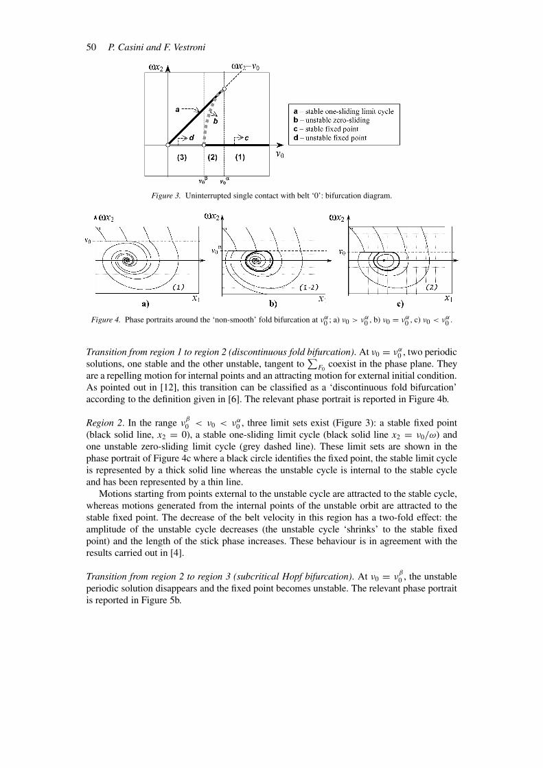
Figure 3. Uninterrupted single contact with belt ‘0’: bifurcation diagram.

Figure 4. Phase portraits around the ‘non-smooth’ fold bifurcation at να0 ; a) ν0 > να

0 , b) ν0 = να0 , c) ν0 < να

0 .

Transition from region 1 to region 2 (discontinuous fold bifurcation). At ν0 = να0 , two periodic

solutions, one stable and the other unstable, tangent to∑

F0coexist in the phase plane. They

are a repelling motion for internal points and an attracting motion for external initial condition.As pointed out in [12], this transition can be classified as a ‘discontinuous fold bifurcation’according to the definition given in [6]. The relevant phase portrait is reported in Figure 4b.

Region 2. In the range νβ

0 < ν0 < να0 , three limit sets exist (Figure 3): a stable fixed point

(black solid line, x2 = 0), a stable one-sliding limit cycle (black solid line x2 = ν0/ω) andone unstable zero-sliding limit cycle (grey dashed line). These limit sets are shown in thephase portrait of Figure 4c where a black circle identifies the fixed point, the stable limit cycleis represented by a thick solid line whereas the unstable cycle is internal to the stable cycleand has been represented by a thin line.

Motions starting from points external to the unstable cycle are attracted to the stable cycle,whereas motions generated from the internal points of the unstable orbit are attracted to thestable fixed point. The decrease of the belt velocity in this region has a two-fold effect: theamplitude of the unstable cycle decreases (the unstable cycle ‘shrinks’ to the stable fixedpoint) and the length of the stick phase increases. These behaviour is in agreement with theresults carried out in [4].

Transition from region 2 to region 3 (subcritical Hopf bifurcation). At ν0 = νβ

0 , the unstableperiodic solution disappears and the fixed point becomes unstable. The relevant phase portraitis reported in Figure 5b.


Figure 5. Phase portraits around the subcritical Hopf bifurcation at νβ0 ; a) ν0 > ν

β0 , b) ν0 = ν

β0 , c) ν0 < ν

β0 .

Region 3. In the range 0 < ν0 < νβ

0 , two limit sets exist (Figure 3): an unstable fixed point(grey solid line, x2 = 0) and a stable one-sliding limit cycle (black solid line x2 = ν0/ω).

These limit sets are shown in the phase portrait of Figure 5c, where a white circle identifiesthe unstable fixed point whereas the stable limit cycle is represented by a thick solid line andis characterized by a slip- and a stick-phase on

∑F0

. Motions starting from points external tothe periodic cycle are attracted to it, whereas motions generated from the internal points arerepelled by the unstable fixed point and collide the limit cycle.

Figures 3–5 have been carried out by using the friction parameters given above; the criticalvalues of the belt velocity are: ν

β

0 = 0.18284 and να0 = 0.26704.

3.3. UNINTERRUPTED DOUBLE CONTACT WITH BOTH BELTS

Now the case σ0 → −∞, σ1 → +∞ is considered; as it has been noted, the mass is alwaysin contact with both belts, for which the same friction parameters have been assumed. Incomparison with the case of uninterrupted single contact analysed previously, the addition ofa second rough support leads to a much richer dynamical behaviour. For given friction anddamping coefficients, the steady state motion of the system depends only upon the drivingvelocities ν0 and ν1. The evolution of steady state attractors as the two driving velocities arevaried will be investigated.

Figure 6 shows a significant portion of the parameter domain (ν0, ν1) where regions ofqualitatively different dynamic responses have been revealed; these regions have been labelledby numerals, furthermore the type of steady-state solutions relevant to each region are reportedin the lower part of the figure. Due to the structure of Equations (11–16) and to the fact thatthe belts possess the same friction parameters, the domain evinces a polar symmetry. Withthe exception of regions 1 and 6, stable limit cycles exhibiting at least one sliding motion arepresent in all other regions: in this connection, letters ‘a’ and ‘b’ label regions in which thestable cycles exhibit sliding in

∑F0

(i.e. the mass sticks on belt 0) and∑

F1(i.e. the mass sticks

on belt 1), respectively, whereas letter ‘c’ labels regions showing evidence of stable cycle withtwo sliding motions (i.e. the mass sticks sequentially on both belts). As it can be deduced fromthe analysis carried out in the previous subsection, sliding motions on a belt are only possibleif its driving velocity is not too high: indeed regions ‘a’ and ‘b’ are located in portions of theparameter domain, where respectively ν0 and ν1 are low. For the same reason, regions ‘c’ arelocated in portions where both ν0 and ν1 are low. Vice versa, if one of the two belts posses ahigh enough driving velocity, the system exhibits dynamical behaviours qualitatively similarto those of the class a) friction oscillator: in fact a sufficiently fast belt adds to the system onlya (constant) damping force.


Figure 6. Uninterrupted double contact with both belts: regions of qualitatively different dynamic responses inthe parameter domain (ν0, ν1).


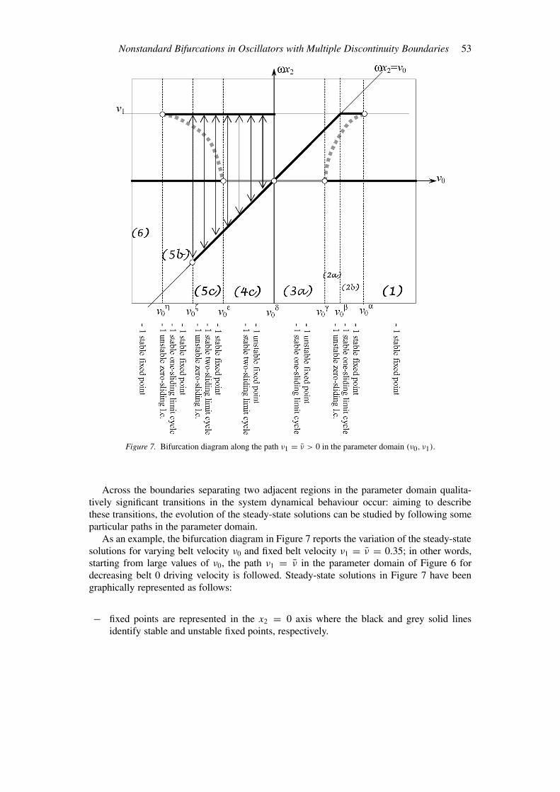
Figure 7. Bifurcation diagram along the path ν1 = ν > 0 in the parameter domain (ν0, ν1).

Across the boundaries separating two adjacent regions in the parameter domain qualita-tively significant transitions in the system dynamical behaviour occur: aiming to describethese transitions, the evolution of the steady-state solutions can be studied by following someparticular paths in the parameter domain.

As an example, the bifurcation diagram in Figure 7 reports the variation of the steady-statesolutions for varying belt velocity ν0 and fixed belt velocity ν1 = ν = 0.35; in other words,starting from large values of ν0, the path ν1 = ν in the parameter domain of Figure 6 fordecreasing belt 0 driving velocity is followed. Steady-state solutions in Figure 7 have beengraphically represented as follows:

− fixed points are represented in the x2 = 0 axis where the black and grey solid linesidentify stable and unstable fixed points, respectively.


Figure 8. Phase portraits around the nonsmooth∑

F1fold bifurcation at να

0 ; a) ν0 > να0 , b) ν0 = να

0 , c) ν0 < να0 .

Figure 9. Phase portraits around the ‘sliding-exchange’ bifurcation at νβ0 ; a) ν0 > ν

β0 , b) ν0 = ν

β0 , c) ν0 < ν

β0 .

Figure 10. Phase portraits around the subcritical Hopf bifurcation at νγ0 ; a) ν0 > ν

γ0 , b) ν0 = ν

γ0 , c) ν0 < ν

γ0 .

Figure 11. Phase portraits around the ‘sudden sliding appearance’ bifurcation at νδ0 = 0; a) ν0 > 0, b) ν0 = 0,

c) ν0 < 0.


Figure 12. Phase portraits around the sliding∑

F0bifurcation at ν

ζ0 ; a) ν0 > ν

ζ0 , b) ν0 = ν

ζ0 , c) ν0 < ν

ζ0 .

Figure 13. Phase portraits around the nonsmooth∑

F1fold bifurcation at ν

η0 ; a) ν0 > ν

η0 , b) ν0 = ν

η0 , c) ν0 < ν

η0 .

− stable steady state-cycles with one or two sliding motions (stick phases) are identified bysolid black lines (distinct from the x2 = 0 axis) which report the variation of the slidingmotion velocity for varying ν0. As it can be noted, in regions 4c and 5c two differentsolid black lines (distinct from the x2 = 0) axis are present: the two lines indicates onlyone stable solution with two different stick phases, one relevant to belt 0 (ωx2 = ν0),the other one relevant to belt 1 (ωx2 = ν1). Since these two lines are associated with aunique stable solution, double arrows linking the lines are added in the diagram.

− unstable steady-state cycles with no sliding motions have been represented via dashedgrey lines: they are only present in regions 2a, b and 5b, c.

Depending on ν0 eight regions of qualitatively different dynamic behaviour do exist:

Region 1. In the range ν0 > να0 only a stable fixed point attractor exists: the relevant phase

portrait is shown in Figure 8a.

Transition from region 1 to region 2b (discontinuous fold bifurcation). At ν0 = να0 , two

periodic solutions, one stable and the other unstable, tangent to∑

F1coexist in the phase plane,

which are a repelling motion for internal points and an attracting motion for external initialcondition. As in the previous subsection, this transition can be classified as a ‘discontinuousfold bifurcation’. The relevant phase portrait is reported in Figure 8b.

Region 2b. In the range νβ

0 < ν0 < να0 , three limit sets exist (Figure 7): a stable fixed point, a

stable one-sliding∑

F1limit cycle and one unstable zero-sliding limit cycle. These limit sets

are shown in the phase portrait of Figure 8c, where a black circle identifies the fixed point, the


stable limit cycle is represented by a thick solid line whereas the unstable cycle is internal tothe stable cycle and has been represented by a thin line. The decrease of the belt velocity inthis region has a two-fold effect: the amplitude of the unstable cycle decreases and the lengthof the stick phase on belt 1 increases.

Transition from region 2b to region 2a (‘Sliding-exchange’ bifurcation). At ν0 = νβ

0 = ν,the two discontinuity boundaries are placed one upon the other. The sliding motions in thestable cycle change: in fact, for values of ν0 larger than ν

β

0 , the stable cycle shows a slidingsolution only in

∑F1

, i.e. the mass sticks on belt 1 (Figure 9a); for values of ν0 smaller than νβ

0 ,the stable cycle shows a sliding solution only in

∑F0

, i.e. the mass sticks on belt 0 (Figure 9c).

Thus, at ν0 = νβ

0 (Figure 9b), a transition occurs since a sliding solution disappears in∑

F1and

appears in∑

F0. This transition is strictly related to the presence of two different discontinuity

boundaries and it will be called ‘sliding-exchange’ bifurcation.

Region 2a. In the range νγ

0 < ν0 < νβ

0 , three limit sets exist: a stable fixed point, a stable one-sliding

∑F0

limit cycle and one unstable zero-sliding limit cycle (Figure 10a). In this regiontoo, the decrease of the belt velocity has a two-fold effect: the amplitude of the unstable cycledecreases (the unstable cycle shrinks to the stable fixed point) and the length of the stick phaseon belt 0 increases.

Transition from region 2a to region 3a (subcritical Hopf bifurcation). At ν0 = νγ

0 , the unstableperiodic solution disappears and the fixed point becomes unstable. The relevant phase portraitis reported in Figure 10b.

Region 3a. In the range 0 < ν0 < νγ

0 , two limit sets exist: an unstable fixed point (greysolid line, x2 = 0 in Figure 7) and a stable one-sliding

∑F1

limit cycle (black solid linex2 = ν0/ω Figure 7). These limit sets are shown in the phase portrait of Figure 10c, where awhite circle identifies the unstable fixed point whereas the stable limit cycle is represented bya thick solid line. Motions starting from points external to the periodic cycle are attracted toit, as motions generated from the internal points which are repelled by the unstable fixed point.

Transition from region 3a to region 4c (‘Sudden sliding appearance’ bifurcation). At ν =νδ

0 = 0, the discontinuity boundary is placed upon the x2 = 0 axis. The fixed points ofthe system are now located in a discontinuity boundary, and can be called pseudoequilibria,according to the definition given in [10]. A segment of pseudo-equilibria does exist (thick linein Figure 11b), which is an attracting set. The sliding motions in the stable cycle change: infact, for values of ν0 larger than νδ

0 = 0 the stable cycle shows a sliding solution only in∑

F0,

i.e. the mass sticks on belt 0 (Figure 11a); for values of ν0 smaller than νδ0 = 0, the stable

cycle shows two different sliding motions in both∑

F0and

∑F1

, i.e. the mass sticks first onbelt 0 then on belt 1 (Figure 11c). Thus, at ν0 = νδ

0 = 0 (Figure 11b), a transition occurs sincea sliding solution suddenly appears in

∑F1

and it will be called ‘sudden sliding appearance’bifurcation.

Region 4c. In the range νε0 < ν0 < νδ

0, two limit sets exist: an unstable fixed point (greysolid line, x2 = 0 in Figure 7) and a stable two-sliding limit cycle (Figure 11c).


Transition from region 4c to region 5c (subcritical Hopf bifurcation). At ν0 = νε0 , an unstable

periodic solution appears and the fixed point becomes stable.

Region 5c. In the range νζ

0 < ν0 < νε0 three limit sets exist: a stable fixed point, a stable limit

cycle with two different stick phases and one unstable zero-sliding limit cycle (Figure 12a).

Transition from region 5c to region 5b (Sliding∑

F0bifurcation). At ν0 = ν

ζ

0 , the stablecycle becomes tangent to the boundary

∑F0

(Figure 12b): since the sliding motion disappearsin

∑F0

, a sliding∑

F0bifurcation is said to occur, according to the definition given in [8].

Region 5b. In the range νη

0 < ν0 < νζ

0 , three limit sets exist: a stable fixed point, a stable limitcycle with only one stick phase on

∑F1

and one unstable zero-sliding limit cycle (Figure 13a).

Transition from region 5b to region 6 (discontinuous fold bifurcation). At ν0 = νη

0 , an unstableperiodic solution tangent to

∑F1

in the phase plane appears, which is a repelling motion forinternal points and an attracting motion for external initial condition. As it has been doneabove, this transition can be classified as a ‘discontinuous fold bifurcation’. The relevant phaseportrait is reported in Figure 13b.

Region 6. In the range ν0 < νη

0 , only a stable point attractor remains: the relevant phaseportrait is shown in Figure 13c.

Figures 6–13 have been carried out by using the same friction parameters for both belts,i.e.: µs0 = µs1 = 1.0, p10 = p11 = 0.60, p20 = p21 = 0, p30 = p31 = 10.0, whereas thenormalised damping coefficient is ζ = 0.50. Critical values of the belt velocity are: να

0 =0.53822, ν

β

0 = 0.35, νγ

0 = 0.26365, νδ0 = 0.0, νε

0 = −0.26365, νζ

0 = −0.4558, and νη

0 =−0.56050.

4. Concluding Remarks

The model of a double-belt friction oscillator has been proposed and investigated in the caseof uninterrupted single contact with only one belt and in the case of uninterrupted doublecontact with both belts; in the latter case multiple discontinuity boundaries appear in the phasespace. The dynamics of this system are of interest because it is a simple representation ofmechanical systems with multiple nonsmooth characteristics and in the same time its responseexhibits nonclassical bifurcation scenarios as a consequence of the occurrence of multiplediscontinuity boundaries caused by the belts. The system exhibits a rich dynamic behaviourand the properties of the limit sets have been found to be different in some ways from those ofsimilar continuous systems. By considering the problem from a nonsmooth dynamical systemsperspective, the evolution of steady state attractors as some system parameters are varied hasbeen investigated by means of numerical and analytical tools.

Nonstandard bifurcations have been detected: as far as the case of uninterrupted singlecontact is concerned, nonstandard phenomena, qualitatively similar to those described in re-cent papers [4, 12], have been recognized. Furthermore, in the case of uninterrupted doublecontact, a much richer dynamical behaviour has been discovered, even in the simple case ofbelts characterized by the same friction parameters.


In the control parameter domain, several regions in which the system exhibits qualitativelydifferent responses have been detected and represented: the characteristic transitions exhibitedby the system across the boundaries separating these regions have been subsequently analysed.In this regard, besides nonstandard phenomena already documented in the literature, somenovel transitions have been detected: in particular, due to the presence of multiple discon-tinuity boundaries, sliding-exchange and sudden sliding appearance bifurcations have beenfound. In the former case, a sliding solution disappears in the discontinuity boundary relatedto a belt and appears in the one related to the other belt. In the latter case, a sliding solutionrelated to a belt abruptly occurs in addition to other sliding motions.

References

1. Filippov, A. F., Differential Equations with Discontinuous Righthand Sides, Kluwer, Dordrecht, TheNetherlands, 1988.

2. Awrejcewicz, J. and Holicke, M. M., ‘Melnikov’s method and stick-slip chaotic oscillations in very weaklyforced mechanical systems’, International Journal of Bifurcations and Chaos 9, 1999, 505–518.

3. Brogliato, B. , Nonsmooth Impact Mechanics, Springer, London, 1999.4. Galvanetto, U. and Bishop, S. R., ‘Dynamics of a simple damped oscillator undergoing stick-slip vibrations’,

Meccanica 34, 1999, 337–347.5. Peterka, F., ‘Analysis of motion of the impact-dry-friction pair of bodies and its application to the investi-

gation of the impact dampers dynamics’, in Proceedings of the ASME 1999 Design Engineering TechnicalConferences, MOVIC’99, Session ‘Friction and Impact Induced Vibrations’, Las Vegas, Nevada, September12–15, 1999, Paper DETC99/ VIB-8350.

6. Leine, R. I., Bifurcations in discontinuous mechanical systems of Filippov-type, Ph.D. Thesis, TechnischeUniversiteit Eindhoven, The Netherlands, 2000.

7. Di Bernardo, M. , Johansson, K. H., and Vasca, F., ‘Self-oscillations in relay feedback systems: Symmetryand bifurcations’, International Journal of Bifurcations and Chaos 11(4), 2001, 1121–1140.

8. Di Bernardo, M., Garofalo, F., Iannelli, L., and Vasca, F., ‘Bifurcations in piecewise-smooth feedbacksystems’, International Journal of Control 75(16), 2002, 1243–1259.

9. Pfeiffer, F. and Glocker, Ch., ‘Contacts in multibody systems’, Journal of Applied Mathematics andMechanics 64(5), 2001, 773–782.

10. Kuznetsov, Yu. A., Rinaldi, S., and Gragnani, A., ‘One-parameter bifurcation in planar Filippov systems’, inProceedings of the Workshop on ‘Bifurcation on Nonsmooth Dynamical Systems’, Milan, Italy, April 22–23,2002.

11. Ivanov, A. P., ‘Impact oscillations: Linear theory of stability and bifurcations’, Journal of Sound andVibration 178(3), 1994, 361–378.

12. Galvanetto, U., ‘An example of a non-smooth fold bifurcation’, Meccanica 36, 2001, 229–233.13. Casini, P. and Vestroni, F., ‘Bifurcations in hybrid mechanical systems with discontinuity boundaries’,

International Journal of Bifurcation and Chaos, 2004, in press.14. Andreaus, U. and Casini, P., ‘On the rocking-uplifting motion of a rigid block in free and forced motion:

influence of sliding and bouncing’, Acta Mechanica 138, 1999, 219–241.15. Lenci, S. and Rega, G., ‘Periodic solutions and bifurcations in an impact inverted pendulum under impulsive

excitation’, Chaos, Solitons and Fractals 11, 2000, 2453–2472.16. Andreaus, U. and Casini, P., ‘Friction oscillators excited by moving base and colliding with rigid or

deformable obstacle’, International Journal of Non-Linear Mechanics 37(1), 2002, 117–133.17. Conti, P., ‘Sulla resistenza di attrito’, Rd. Acc. Lincei 11, 1875.18. Popp, K., Hinrichs, N., and Oestreich, M., ‘Analysis of a self-excited friction oscillator with external excita-

tion’, in Dynamics with Friction, A. Guran, F. Pfeiffer, and K. Popp (eds.), World Scientific, London, 1996,pp. 1–35.

19. Shaw, S. H., ‘On the dynamic response of a system with dry friction’, Journal of Sound and Vibration 108(2),1986, 305–325.

20. Leine, R. I., Van Campen, D. H., De Kraker, A., and Van Den Steen, L., ‘Stick-slip vibration induced byalternate friction models’, Nonlinear Dynamics 16, 1998, 41–54.


21. Andreaus, U. and Casini, P., ‘Dynamics of friction oscillators excited by moving base or/and driving force’,Journal of Sound and Vibration 245(4), 2001, 685–699.

22. Utkin, V. I., Sliding Modes in Control Optimization, Springer, Berlin, 1992.23. Kuznetsov, Yu. A. and Levitin, V. V., ‘CONTENT: A multiplatform environment for analyzing dynamical

systems’, Technical Report, Dynamical Systems Laboratory, CWI, Amsterdam, 1997.

Nonstandard Bifurcations in Oscillators with Multiple Discontinuity Boundaries

Documents

Transcript of Nonstandard Bifurcations in Oscillators with Multiple Discontinuity Boundaries