Complex variations in sediment transport at three large river bifurcations during discharge waves in...

57

Complex variations in sediment transport at three

large river bifurcations during discharge waves in

the river Rhine

Roy Frings and Maarten Kleinhans

Accepted for publication in Sedimentology

Abstract

River bifurcations strongly control the distribution of water and sediment over a river system. A

good understanding of this distribution process is crucial for river management. In this paper an

extensive dataset from 3 large bifurcations in the Dutch Rhine is presented, containing data on

bed-load transport, suspended bed sediment transport, dune development and hydrodynamics.

The data show complex variations in sediment transport during discharge waves. The objective of

this chapter is to examine and explain these measured variations in sediment transport. It is

found that bend sorting upstream of the bifurcations leads to supply limitation, particularly in the

downstream branch that originates in the outer bend of the main channel. Tidal water level

variations lead to cyclical variations in the sediment distribution over the downstream branches.

Lags in dune development cause complex hysteresis patterns in flow parameters and sediment

transport. All bifurcations show evidence of sediment waves, which probably are intrinsic

bifurcation phenomena. The complex transport processes at the three bifurcations cause distinct

discontinuities in the downstream fining trend of the river. Differences among the studied river

bifurcations are mainly due to differences in sediment mobility (Shields value). Because the

variations in sediment transport are complex and poorly correlated with the flow discharge,

prediction of the sediment distribution with existing relations for 1D models is problematic.

3.1 Introduction

Flow bifurcations are typical features of braided rivers, alluvial fans and river deltas, and strongly

determine the stability of a river system. A change in sediment distribution at a river bifurcation

often leads to aggradation in one of the downstream branches. At the same time, the water

discharge through this branch will decrease, while the water discharge through the other branch

increases. This affects the flooding risk and navigability of both branches, as well as the

availability of water for vegetational, agricultural and human needs. A good understanding of the

sediment distribution process at river bifurcations thus is crucial for river management.

3

Frings - From gravel to sand

58

In recent years, considerable progress was made with theoretical bifurcation studies and

laboratory experiments (e.g. Bolla Pittaluga et al., 2003; Federici and Paola, 2003), but a major

drawback of these studies is that they all refer to highly idealised situations, usually with constant

discharge, constant water levels, uniform sediment and an absence of dune-type bedforms.

Important questions thus remain unanswered. How do bifurcations behave during discharge

waves? What are the effects of bend sorting upstream of a bifurcation on the sediment

distribution? How do tidal water level variations affect this distribution? How does the dune

development interact with the sediment transport?

To study these controls on bifurcation behaviour, decades of field measurements were done in

the river Rhine. An overview of the major field campaigns is presented here. The objective of this

paper is to examine and explain the variations in sediment transport at the three largest river

bifurcations during discharge waves. In particular, the following hypotheses are tested (Fig. 3.1):

(1) Bend sorting upstream of a bifurcation causes supply-limited transport conditions in one

of the downstream branches.

(2) Tidal water level fluctuations cause cyclical variations in sediment distribution at river

bifurcations.

(3) The delayed adaptation of dunes after a change in flow conditions causes hysteresis in

hydraulic roughness and bed-load transport.

The rationale behind these hypotheses is as follows.

(1) In meander bends, bend sorting causes a segregation of coarse grains in the outer bend

and fine grains in the inner bend. This often leads to relatively low bed-load transport rates in the

outer bend (e.g. Dietrich and Whiting, 1989). The coarse sediments in the outer bend may even be

completely immobile during a considerable part of the year, while the fine sediments in the inner

bend are constantly in motion. This inevitably affects the sediment distribution at a river

bifurcation that is situated downstream of a meander bend. It is likely that the river branch that

connects to the coarse-grained outer bend of the main channel receives a low bed-load supply

from upstream, even if the water supply is large (Fig. 3.1a). This implies that the flow in this

branch is able to transport more bed load than is supplied from upstream, a situation generally

known as supply-limited transport. It is probable that bend sorting upstream of a river bifurcation

only leads to supply limitation if the Shields value at the bifurcation is low. At high Shields values,

all grain size fractions will be fully mobile, and the sediment distribution will be unaffected by

bend sorting upstream of the bifurcation.

(2) In coastal areas, the effects of bend sorting on the sediment distribution may be overruled

by tidal effects. Both downstream branches of a river bifurcation commonly end up in the same

water body. Tidal fluctuations of the water level in this water body propagate upstream to the

bifurcation through both branches. Due to differences in length and flow resistance between the

two branches, it is likely that the tidal effect of one of the branches is dominant. When the tide


59

comes in through this branch, the water and sediment discharge through this branch is

hampered, while the water and sediment discharge through the other branch is promoted (Fig.

3.1b). At outgoing tide the situation probably is reverse, so that the distribution of water and

sediment at the bifurcation cyclically varies during a tidal cycle.

(3) The bed-load transport at river bifurcations may be further complicated by dune

development. Dunes cannot quickly adapt to changing flow conditions. Especially the dune

length often lags behind changes in discharge (e.g. Wilbers and Ten Brinke, 2003), causing dunes

to be steeper before the peak discharge than thereafter. Therefore, the dune steepness is expected

to follow a clockwise hysteresis (Fig. 3.1c). Because the hydraulic roughness is positively

correlated with the dune steepness (e.g. Yang et al., 2005), also the hydraulic roughness is

expected to follow a clockwise hysteresis (Fig. 3.1c). Changes in hydraulic roughness have a

complex effect on the flow conditions and bed-load transport. Nevertheless, it is often supposed

Figure 3.1 Hypotheses regarding the sediment transport at river bifurcations. (a) Hypothesis 1: bend sorting

upstream of a bifurcation causes supply-limited transport conditions in one of the downstream branches.

(b) Hypothesis 2: tidal water level fluctuations cause cyclical variations in sediment distribution at river

bifurcations. (c) Hypothesis 3: dunes only slowly adapt to changing flow conditions, causing a hysteresis in

hydraulic roughness and bed-load transport.


60

Figure 3.2 Topography, median grain size and measurement sites at the studied river bifurcations: (a)

Pannerdensche Kop, (b) IJsselkop and (c) Merwedekop. (Grain size information after Gruijters et al., 2001,

2003; Frings, 2005b).


61

that hysteresis in hydraulic roughness causes an opposite hysteresis in bed-load transport (e.g.

Kleinhans, 2005c), by reasoning that a decrease in roughness reduces the amount of bed shear

stress needed to overcome bed friction, leaving a larger part available for bed-load transport, and

therefore increasing the bed-load transport (Fig. 3.1c).

In this paper, first a description is given of the three bifurcations and the measurement

techniques. Then, the field data on flow conditions, sediment mobility, dune development and

sediment transport are presented. Next, the three hypotheses regarding bend sorting, tides and

transport hysteresis are discussed. Afterward, evidence is summarised for the presence of

sediment transport waves, which seem to be intrinsic part of all three bifurcations, and possible

explanations are evaluated. Finally, the implications of all these bifurcation controls for the

prediction of the sediment distribution at bifurcations are discussed, as well as their influences on

downstream fining patterns.

3.2 Rhine bifurcations

The river Rhine originates in the Swiss Alps, passes Germany and The Netherlands, and ends,

after 1320 km, in the North Sea. In The Netherlands, the Rhine splits into several branches (Fig.

3.2, inset). The main bifurcations are the Pannerdensche Kop, the IJsselkop and the Merwedekop,

which are the subject of this study.

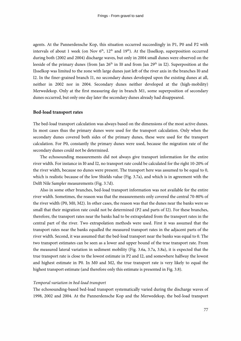
At the first two bifurcations, the river bed consists of a low-mobility sand-gravel mixture, but

at the Merwedekop, the river bed consists of highly mobile sand (Fig. 3.3). The water distribution

at the Pannerdensche Kop is more or less constant over time, but the distribution at the IJsselkop

strongly varies between high-flow and low-flow periods because one of the downstream branches

contains weirs that are partly closed during low-flow periods. The water distribution at the

Merwedekop is variable and depends on the regulation of the Haringvlietsluices, on the wind

direction and especially on the semi-diurnal tides (Fig. 3.3).

To allow easy comparison of the bifurcations, their river branches are coded with a letter (P, I

or M) referring to the bifurcation and a number (0, 1 or 2) referring to the size of the branch (Fig.

3.2). For instance, the largest branch at the Pannerdensche Kop is called P0 and the smallest

branch at the Merwedekop M2.

The average annual discharge of the Rhine near the German-Dutch border is 2,300 m3 s-1,

stemming from both rain and snowmelt. The maximum discharge ever recorded was 12,600 m3 s-1

in 1926 AD. The flow depth varies between 3 and 12 m between low-flow and high-flow periods.

The width of the rivers between the groynes varies between 64 m and 440 m (Fig. 3.3). All Rhine

branches are heavily engineered: banks are protected with groynes, shipping routes are constantly

being dredged and embankments prevent flooding of the densely populated areas near the river.

The plan form of the branches is meandering. Despite a relatively low sinuosity, most meander

bends show a strong bend-sorting pattern, with fine grains in the inner bend and coarse grains in

the outer bend. Bend sorting upstream of the bifurcations causes grain-size differences between


62

the bed sediments at the entrance of the two downstream branches, as was revealed by 156 vibra-

cores and 92 grab samples that were taken on the river bed in 2000, 2002 and 2004 AD (Fig. 3.2,

Gruijters et al., 2001, 2003; Frings, 2005b).

3.3 Field measurements

Measuring campaigns

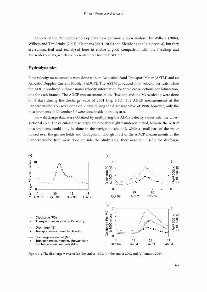
Field measurements at the Pannerdensche Kop bifurcation were done during the discharge wave

of November 1998, which had a peak discharge of 9600 m3 s-1 in the Bovenrijn (P0) with a

recurrence interval of about 20 years (Fig. 3.4a). The main field campaigns at the IJsselkop and

Merwedekop took place during the short discharge wave of January 2004 (Fig. 3.4c). During this

wave a peak discharge in P0 was reached of 6740 m3 s-1, with a recurrence interval of about 2

years. During all field campaigns comprehensive measurements of bed-load transport, suspended

load transport and hydrodynamics were done. At the IJsselkop, additional measurements were

done during the discharge wave of November 2002 (Fig. 3.4b) and the low-flow period of

September 2004. The peak discharge in 2002 was almost equal to that in 2004, 6490 m3 s-1; the

discharge during the low flow period was 1600 m3 s-1.

Figure 3.3 Basic characteristics of the studied river bifurcations. Indicated are the width-averaged median

grain size of each branch (D) (based on Gruijters et al., 2001, 2003 and Frings, 2005b), the width of each

branch (W), and the proportion of water that flows into the largest branch.


63

Aspects of the Pannerdensche Kop data have previously been analysed by Wilbers (2004),

Wilbers and Ten Brinke (2003), Kleinhans (2001, 2002) and Kleinhans et al. (in press, a), but they

are summarised and reanalysed here to enable a good comparison with the IJsselkop and

Merwedekop data, which are presented here for the first time.

Hydrodynamics

Flow velocity measurements were done with an Acoustical Sand Transport Meter (ASTM) and an

Acoustic Doppler Current Profiler (ADCP). The ASTM produced flow velocity verticals, while

the ADCP produced 2-dimensional velocity information for three cross sections per bifurcation,

one for each branch. The ADCP measurements at the IJsselkop and the Merwedekop were done

on 5 days during the discharge wave of 2004 (Fig. 3.4c). The ADCP measurements at the

Pannerdensche Kop were done on 7 days during the discharge wave of 1998; however, only the

measurements of November 3rd were done inside the study area.

Flow discharge data were obtained by multiplying the ADCP velocity values with the cross-

sectional area. The calculated discharges are probably slightly underestimated, because the ADCP

measurements could only be done in the navigation channel, while a small part of the water

flowed over the groyne fields and floodplains. Though most of the ADCP measurements at the

Pannerdensche Kop were done outside the study area, they were still useful for discharge

Figure 3.4 The discharge waves of (a) November 1998, (b) November 2002 and (c) January 2004.


64

determination. If ADCP data were unavailable, the flow discharge was derived from rating curves

at automatic gauging stations.

The water level slope at the Pannerdensche Kop was determined from height measurements

at automatic gauging stations situated at a distance of 0.3 km (P0), 5.3 km (P0), 17.4 km (P1) and

11.1 km (P2) from the bifurcation. For the IJsselkop and Merwedekop, the slope was determined

from water level measurements with gauges that were installed at regular distances of each other

at both sides of the river, from approximately 1 km upstream of the bifurcation to approximately

1 km downstream of the bifurcation.

Sediment mobility determination

The flow measurements were used to determine the sediment mobility:

2

250

'' ( 1)

uθ

C s D=

− (3.1)

with θ’ the Shields mobility parameter (related to skin friction), ū the depth-averaged flow

velocity (m s-1), s the relative sediment density (=ρs / ρ), ρ and ρs respectively the density of water

and sediment (kg m-3) and C’ the Chezy skin friction factor (m0.5 s-1). C’ was calculated as C’ =

18log(12H/ks’), with H the flow depth (m) and ks’ the Nikuradse grain roughness (m) (ks’=D90, cf.

Kleinhans and Van Rijn, 2002). D50 and D90 are respectively the 50th and 90th percentile of the bed

grain size distribution and were taken from grab samples (Merwedekop) or interpolated vibra-

cores (other bifurcations). H and ū were taken from ASTM measurements (P1) or ADCP

measurements (other branches). Both methods give the same results (Fig. 3.8a). In case ADCP

measurements were used, calculated Shields values are representative for a 20 m wide zone; if

ASTM measurements were used, Shields values are only valid locally.

Bed-load transport

Two methods were used to determine the bed-load transport at the bifurcations: (1)

echosoundings and (2) bed-load samplers. The echosounding method calculates the bed-load

transport from the size and migration rate of the subaqueous dunes. This method gives detailed

information on the spatial variation in bed-load transport, but only if the bed-load transport

occurs by moving dunes. Bed-load samplers give direct information on the transport rate (even if

dunes are absent), but the spatial resolution is limited. However, samplers also provide

information on the grain-size composition of the transport material. The combination of

echosoundings and bed-load samplers therefore gives the most accurate estimate of the bed-load

transport.


65

Bed-load transport from echosoundings

Echosoundings were carried out during the discharge waves of 1998 (Pannerdensche Kop), 2002

(IJsselkop) and 2004 (IJsselkop and Merwedekop) on 3-12 days per discharge wave (Fig. 3.4). The

measurements were done 2 or 3 times a day, in order to assure that the displacement of dunes

between two echosoundings was not more than one dune length, for this would have hampered

the transport computation (Wilbers and Kleinhans, 1999).

The echosoundings covered the full river width between the groynes, from about 1 km

upstream of the bifurcation, to 1 km downstream of the bifurcation. In some branches (M0, M2,

P0), the echosoundings were limited to the central 70% of the river width.

Most of the echosoundings were done with a multibeam echosounding system, which scans

the bed topography in a line perpendicular to the track of the survey vessel. While the vessel was

moving, a strip river bed was scanned with a width equal to several times the water depth. By

sounding several vessel tracks parallel to the banks, area-covering bed elevation data were

obtained. In branch P2 some of the measurements were done with a single-beam echosounding

system. This system only gives information on the bed topography directly underneath the vessel.

By situating the single-beam tracks 10 metres apart and parallel to the banks, however, still

detailed information on the spatial variation in dune characteristics could be determined. More

information on the used echosounding systems is given by Wilbers and Ten Brinke (2003).

The obtained echosounding data were divided into subreaches with a width equal to the river

width and a length of 400-1000 m (Fig. 3.2). For each subreach and each measuring day, the size

and migration rate of the dunes were calculated using the dune tracking software DT2D (Ten

Brinke et al., 1999). In DT2D, two-dimensional longitudinal profiles were constructed out of the

echosounding data with a spacing of 1-10 m (respectively for multibeam and single-beam

echosoundings). Through each longitudinal profile a moving average was computed, and each

part of the profile below the moving average was identified as a dune trough. For each dune, the

Figure 3.5 Definition of dune dimensions and overestimation in dune dimensions due to stochastic errors

(noise) in echosoundings. The overestimation in dune height is equal to 2 times the noise, the

overestimation in cross-sectional area is equal to the product of dune length and noise. The dune length

itself is not systematically affected by noise.


66

length, height and cross-sectional area were determined (Fig. 3.5). By comparing the longitudinal

profiles of 2 consecutive echosoundings with a cross-correlation technique (Ten Brinke et al.,

1999), also the migration rate of the dunes was determined.

The longitudinal resolution of the echosounding data (1.7–5 points per metre) determines a

minimum dune size that can accurately be determined with DT2D. For the IJsselkop and

Merwedekop, the minimum dune length was estimated at respectively 1 and 2 m; shorter dunes

were deleted from the dataset. Apart from the short dunes, also the 0.5% largest dunes were

deleted from the dataset (outliers). Furthermore all dunes that consist of less than 1 point per

metre dune length were deleted. For the Pannerdensche Kop, a different procedure was used.

Wilbers and Ten Brinke (2003) removed all dunes consisting of less then 10 data points from the

dataset, because their dune dimensions were considered inaccurate. This caused a slight

overestimation of the dune dimensions, because many dunes in the Rhine are small (1-5 m) and

therefore covered by less than 10 points.

Because echosoundings contain a stochastic measuring error (noise) of about 2 cm, the dune

dimensions are overestimated by DT2D. All dunes of the IJsselkop and Merwedekop were

corrected for this overestimation (Fig. 3.5). Next, the average length and height of the dunes in a

longitudinal profile were calculated from the individual dunes.

The average bed-load transport in a longitudinal profile was calculated using the following

equation (based on Ten Brinke et al., 1999):

Δbq c β= ⋅ ⋅ (3.2)

with qb the specific bed-load transport including pores (m2 day-1), c the dune migration rate (m

day-1), Δ the dune height (m) and β the bed-load discharge coefficient (-). Equation 3.2 is only

valid if the net bed-load transport perpendicular to the main flow direction is zero and the

average bed level is constant. The coefficient β combines corrections for the dune shape, for

trough-bypassing transport and for the fact that the position of zero bed-load transport is not the

dune trough but the reattachment point. Wilbers (2004) demonstrated that for the Dutch Rhine

branches β≈0.5F, with F a shape factor (-), equal to the ratio between the cross-sectional area of a

dune and the cross-sectional area of a triangular dune with the same length and height. For the

Pannerdensche Kop dataset, F was set equal to 1.10; for the IJsselkop and Pannerdensche Kop

datasets, F was determined empirically using DT2D, giving values between 1.03 and 1.17.

After calculating the bed-load transport for each longitudinal profile (using profile-averaged

values for c, Δ and F), the width-averaged bed-load transport was calculated by integration over

the cross-section.

Bed-load transport from bed-load samplers

In addition to echosoundings, also bed-load samplers were used to determine the bed-load

transport during the discharge waves of 1998 (Pannerdensche Kop) and 2004 (IJsselkop and


67

Merwedekop). The measurements were done in cross-sections of the branches P1, I0 and M0

(Fig. 3.2a-c) on several days (Fig. 3.4). During the low-flow period of September 2004 a limited

number of sampler measurements were done in the 3 branches of the IJsselkop (Fig. 3.2b).

For the measurements at the Pannerdensche Kop an adapted version of the Helley-Smith bed-

load sampler was used (Kleinhans and Ten Brinke, 2001). This sampler had an orifice size of 7.62

x 7.62 cm and a mesh diameter of 250 μm. Since 1998 it has become clear that its trapping

efficiency in sand-gravel bed rivers is not optimal, resulting in a relatively high calibration factor

of 2.7 (Kleinhans, 2002). Therefore at the IJsselkop and Merwedekop in 2004 another sampler was

used, the Delft Nile Sampler (Van Rijn and Gaweesh, 1992; Gaweesh and Van Rijn, 1994). This

sampler has a calibration factor of 1 ± 0.1 (Van Rijn and Gaweesh 1992; Kleinhans and Ten

Brinke, 2001). The orifice of the Delft Nile Sampler was 9.8 cm wide and 5 cm high. The orifice

height of both samplers was somewhat larger than the thickness of the bed-load layer, so the

samplers also captured some suspended load transport. For practical reasons, however, all

sediment measured with the samplers is considered to be bed-load transport.

To measure the bed-load transport in a cross-section, the cross-section was divided in several

subsections. For the Pannerdensche Kop and the Merwedekop 7 subsections were used; for the

IJsselkop 5 subsections in the upstream branch and 3 subsections in the smaller downstream

branches (Fig. 3.2). In each subsection 20 bed-load transport samples were taken from the same

anchoring position. The sample duration was 2 minutes. If the transport rate was very low, the

number of samples was reduced, but the sample duration increased, to ensure a sufficient filling

of the sample bag. Of each sample the volume was measured as well as the grain-size distribution

(by sieving).

To test whether the samples were disturbed by scooping and whirling during the touchdown

and rising of the bed-load sampler, the sampler was lowered and pulled up 5 times quickly after

each other in every subsection, after which the volume of sediment in the sample bag was

measured. This revealed that only the transport samples at the fine-grained Merwedekop were

disturbed and had to be corrected. After correction, all sample volumes were translated into bed-

load transport rates, using a calibration factor 1.0 for the Delft Nile Sampler and a factor 2.7 for

the adapted Helley-Smith Sampler. These transport rates per subsection were integrated to get the

total bed-load transport through the cross section.

Suspended load transport

Every bed-load sampler measurement was accompanied by a simultaneous measurement of the

suspended load transport using an Acoustical Sand Transport Meter (ASTM). The ASTM is not

sensitive to clay and silt-sized particles, thus it does not measure wash-load transport. The term

‘suspended load transport’ in this paper consequently always refers to the suspended load

transport of bed material (above the top of the bed-load sampler). At each location, the suspended

load was measured at several positions in the water column (0.2, 0.5, 1, 2 and 3 m above the bed,


68

and so on up to the water surface), after which the total suspended load transport in the water

column was determined by integration. To obtain grain-size information of the suspended load,

water samples were taken using a Pump Filter System (PFS) close to the measuring spot of the

ASTM. The water was led over a filter with a mesh size of 50 μm to exclude wash load from the

sediment sample. The grain-size distribution of the sediment was determined in the two-metre

long settling tube of the Department of Physical Geography at Utrecht University, The

Netherlands.

Accuracy analysis

The accuracy of the transport rates is affected by systematic and stochastic measuring errors and

by natural variability in transport rates (Kleinhans and Ten Brinke, 2001). Systematic measuring

errors are accounted for by the calibration factors of the measurement instrument and

techniques. The uncertainty induced by stochastic measuring errors and natural variability is

calculated separately for the sampler-based transport measurements and the echosounding-based

transport measurements.

Sampler-based measurements are affected by stochastic errors that originate mainly from

uncertainties in the positioning of the instrument and from uncertainties in determining

sampling time and volume. These stochastic measuring errors are in practice not distinguishable

from small-scale natural variability in sediment transport due to for instance turbulence and the

presence of dunes. Both types of errors cause differences between transport rates that are

measured shortly after each other in the same subsection. The uncertainty involved is equal to the

standard error of the measuring values. Using standard analytical error propagation formulae (cf.

Kleinhans and Ten Brinke, 2001) the subsection uncertainties were combined into the uncertainty

for the cross-section-integrated transport.

Echosounding-based measurements are affected by stochastic errors in the echosounding

system that cause a noise around the bed elevation data. This noise leads to a systematic

overestimation of the dune dimensions (Fig. 3.5), but is sometimes also detected as separate small

‘dunes’ by the dune tracking software DT2D. For the IJsselkop and Merwedekop datasets, these

errors have been minimised by applying a correction to the dune dimensions (Fig. 3.5), and by

deleting all dunes shorter than 1-2 m from the dataset. In the already existing Pannerdensche Kop

dataset (Wilbers, 2004), these corrections have not been applied, probably leading to a slight

overestimation in transport.

Echosounding-based measurements are also affected by uncertainties in the profile-averaged

dune height that arise because DT2D was not always able to determine the height of all individual

dunes in a longitudinal profile. These uncertainties were quantified according to the procedure

described in Frings (2005a,b) and combined with the uncertainty in the migration rate into an

uncertainty value for the cross-section averaged bed-load transport rate.


69

In deriving the uncertainty values, it was assumed that the hydrodynamic conditions were

constant during one set of measurements in a cross section and that the transport rate varied

linearly between 2 measurement locations. For simplicity it was assumed that all uncertainties are

mutually independent.

3.4 Results

The results of the bifurcation measurements are graphically presented in Fig. 3.6 - 3.9 and

summarised in Appendix 3.

Sediment mobility

The sediment mobility significantly differs between the bifurcations (Fig. 3.6a, 3.7a, 3.8a). The

Merwedekop has the highest and the IJsselkop the lowest mobility, with respective (grain) Shields

values of about 0.23 and 0.07. At the Pannerdensche Kop, the sediment mobility greatly varies

between the branches. P2 has a low (grain) Shields value (about 0.05), while P0 and P1 have

notably larger (grain) Shields values (respectively 0.13 and 0.28 during the peak discharge).

At the Pannerdensche Kop and IJsselkop, the sediment mobility strongly varied over the river

width, with the highest values generally around the river axis. Especially remarkable are the low-

mobility zones at the right side of P0 and I0. These zones correspond to the outer meander bend,

and are situated exactly at the entrance of the branches P2 and I2 (in these branches the mobility

is also extremely low). There are some indications that the low-mobility zones near the right

banks of P0 and I0 increase in width as the discharge decreases (e.g. Fig. 3.7a).

Dune patterns

In some branches of the Pannerdensche Kop and Merwedekop (P1, P2 and M1), the entire river

width was covered with dunes. In the other branches (P0, M0, M2), dunes covered at least the

central 70-80% of the river width. Whether dunes were present near the banks could not be

determined, because the echosoundings did not span the entire river width. At the IJsselkop,

dunes covered the entire river width in I1, but only the left 80-90% of the river width in I0 and I2.

The dune dimensions at the Merwedekop, which is characterised by a high sediment mobility,

did hardly vary over the measured part of the river width. The same is true for the dune

dimensions in the high-mobility branches of the Pannerdensche Kop (P0, P1). In the low-

mobility branch P2 there was a strong lateral variation in dune dimensions, with high values in a

40-50 m wide zone just left of the river axis, and low values outside this zone. Also at the (low-

mobility) IJsselkop, there was a strong variation in dune length and dune height over the river

width, with the highest values just right of the river axis (I1) or just left of it (I0 and I2). The dunes

close to the edges of the dune zone were sometimes so small and irregular, that their dimensions


70

Figure 3.6 The Pannerdensche Kop dataset.

(a) Variation in critical Shields value (θc) and Shields value due to skin friction (θ´) in the branches P0 (km

867.5), P1 (km 868.5) and P2 (km 869.0).

(b) Temporal variation in width-averaged dune height (Δ).

(c) Temporal variation in bed-load transport based on echosoundings (qb). For the river branches P0 and

P2 the minimum and maximum transport estimates are shown.


71

Figure 3.6 (continued)

(d) Upper panel: lateral variation in bed-load transport based on echosoundings (qb), during the peak

discharge.

Lower panel: lateral variation in D90 of bed-load material and bed material.

(e) Variation in sediment transport as function of discharge. Bed-load data (qb) are obtained from echo-

soundings (ES) or Helley-Smith samplings (HS), suspended load data (qs) from ASTM measurements.

(f) Supply of discharge (Q) and width-integrated bed-load transport (Qb) into branch P2, expressed as

percentage of the summed transport in branch P1 and P2. Four different estimates of the Qb-supply are

shown. For estimates 1 and 2, the Helley-Smith-based transport rates from P1 were used in

combination with respectively the maximum and minimum echosounding-based transport rates from

P2. For estimates 3 and 4 the same transport rates from P2 were used, in combination with the

echosounding-based transport rates from P1.


72


73

Figure 3.7 The IJsselkop dataset.

(a) Variation in critical Shields value (θc) and Shields value due to skin friction (θ´) in the branches I0 (km

878.0), I1 (km 879.5) and I2 (km 879.5).

(b) Temporal variation in width-averaged dune height (Δ).

(c) Temporal variation in bed-load transport rate (qb) based on Delft Nile Sampler (DNS) measurements

and echosoundings (ES) in the subreaches A-I (see Fig. 3.2). For the subreaches G, H and I the

minimum and maximum transport estimate are shown.

(d) Upper panel: lateral variation in bed-load transport (qb) during the peak discharge. For branch I0, I1

and I2, ES-data from subreach A, E and H are shown. For branch I0 also DNS-data are shown

Lower panel: lateral variation in D90 of bed-load material and bed material (axis on the right).

(e) Variation in sediment transport as function of the water discharge in January 2004.

(f) Supply of discharge (Q) and width-integrated bed-load transport (Qb) into branch I2, expressed as

percentage of the summed transport in branch I1 and I2. Two different estimates of the Qb-supply are

shown. For estimate 1 and 2, the echosounding-based transport rate from subreach D was used in combination with respectively the maximum and minimum estimate of the transport in subreach G.


74

Figure 3.8 The Merwedekop dataset.

(a) Variation in critical Shields value (θc) and Shields value due to skin friction (θ´) in the branches M0

(km 960.5-960.8), M1 (km 962.0) and M2 (km 961.7). Maximum and minimum values during a tidal

cycle are shown (based on ADCP measurements). For comparison one value based on ASTM

measurements is shown. The available grain size data did not allow calculation of the Shields value

near the banks; as surrogate the change of ADCP flow velocity towards the banks is shown (arrow).

(b) Temporal variation in the width-averaged dune height (Δ).

(c) Temporal variation in bed-load transport (qb) based on ES and DNS measurements.

(d) Upper panel: lateral variation in bed-load transport (qb) based on echosoundings (averaged over the

discharge wave). Lower panel: lateral variation in D50 of bed-load material and bed material.

(e) Variation in sediment transport as function of the water discharge.

(f) Supply of width-integrated bed-load transport (Qb) into branch M2.

(g) Tidal variation in relative bed-load transport (instantaneous transport/tidal-average transport).


75


76

and migration could not be determined. This was especially the case in branch I2, where near the

left bank a zone immeasurable dunes occurred, with a width of about 25% of the dune zone width.

At all three bifurcations, the dunes upstream of the bifurcation were higher than those

downstream of it.

Dune growth and decay

During the discharge wave of 1998 (on October 30th), the dunes at the Pannerdensche Kop grew

to a maximum height of 49-120 cm (Fig. 3.6b). In P2, especially the dunes left of the river axis

grew (to a maximum of 72 cm). In all branches the maximum dune height was reached within 3

days after the peak discharge. From then on, the dune height gradually decreased. In the high-

mobility branch P1, the dune length also decreased, but much faster, making the dunes steeper. In

the low-mobility branches P0 and P2, the dune length did not decrease and the dunes became less

steep (Fig. 3.9a).

The dunes at the IJsselkop were generally much smaller than the dunes at the Pannerdensche

Kop (Fig. 3.7b). In the branches I0 and I2 especially the dunes just left of the river axis grew

during the discharge wave of 2004 (to a maximum of 23-50 cm). After the peak discharge the

dune length kept increasing just left of river axis, but decreased elsewhere. Also the dune height

gradually decreased, causing a net decrease in dune steepness (Fig. 3.9b). The dune development

in I1 was more complex. Close to the bifurcation, the dunes grew during rising discharges and

became smaller after the discharge peak, just as in I0 and I2. Only 800 m downstream, however,

the dune development was exactly reverse: the dunes became smaller during rising flow and

started to grow when the discharge decreased (Fig. 3.7b). During the discharge wave of November

2002, the dune development was largely the same as described above, but the dunes attained a

larger maximum height (Fig. 3.7b).

At the Merwedekop, the dunes had similar dimensions as at the IJsselkop. During the

discharge wave of 2004, the dunes grew to a maximum height of 27-40 cm (Fig. 3.8b). After the

peak discharge, the dune length continued to increase very slowly, whereas the dune height

gradually decreased, causing the dunes to become steeper (Fig. 3.9c).

Superposition

At the (low-mobility) bifurcations Pannerdensche Kop and IJsselkop, the primary dunes that

were described in the previous paragraph, became covered with small, secondary dunes during

the period of receding flow. Initially these secondary dunes plunged down the leeside of the

primary dunes and developed again on the stoss side of the next primary dune, so allowing

movement of the primary dunes. After a few days, however, the secondary dunes increasingly

travelled over the lee sides of the primary dunes without being broken up, which indicates that the

primary dunes became inactive, while the secondary dunes became the main bed-load transport


77

agents. At the Pannerdensche Kop, this situation occurred succeedingly in P1, P0 and P2 with

intervals of about 1 week (on Nov 6th, 12th and 19th). At the IJsselkop, superposition occurred

during both (2002 and 2004) discharge waves, but only in 2004 small dunes were observed on the

leeside of the primary dunes (from Jan 26th in I0 and from Jan 29th in I2). Superposition at the

IJsselkop was limited to the zone with large dunes just left of the river axis in the branches I0 and

I2. In the finer-grained branch I1, no secondary dunes developed upon the existing dunes at all,

neither in 2002 nor in 2004. Secondary dunes neither developed at the (high-mobility)

Merwedekop. Only at the first measuring day in branch M1, some superposition of secondary

dunes occurred, but only one day later the secondary dunes already had disappeared.

Bed-load transport rates

The bed-load transport calculation was always based on the dimensions of the most active dunes.

In most cases thus the primary dunes were used for the transport calculation. Only when the

secondary dunes covered both sides of the primary dunes, these were used for the transport

calculation. For P0, constantly the primary dunes were used, because the migration rate of the

secondary dunes could not be determined.

The echosounding measurements did not always give transport information for the entire

river width. For instance in I0 and I2, no transport rate could be calculated for the right 10-20% of

the river width, because no dunes were present. The transport here was assumed to be equal to 0,

which is realistic because of the low Shields value (Fig. 3.7a), and which is in agreement with the

Delft Nile Sampler measurements (Fig. 3.7d).

Also in some other branches, bed-load transport information was not available for the entire

river width. Sometimes, the reason was that the measurements only covered the central 70-80% of

the river width (P0, M0, M2). In other cases, the reason was that the dunes near the banks were so

small that their migration rate could not be determined (P2 and parts of I2). For these branches,

therefore, the transport rates near the banks had to be extrapolated from the transport rates in the

central part of the river. Two extrapolation methods were used. First it was assumed that the

transport rates near the banks equalled the measured transport rates in the adjacent parts of the

river width. Second, it was assumed that the bed-load transport near the banks was equal to 0. The

two transport estimates can be seen as a lower and upper bound of the true transport rate. From

the measured lateral variation in sediment mobility (Fig. 3.6a, 3.7a, 3.8a), it is expected that the

true transport rate is close to the lowest estimate in P2 and I2, and somewhere halfway the lowest

and highest estimate in P0. In M0 and M2, the true transport rate is very likely to equal the

highest transport estimate (and therefore only this estimate is presented in Fig. 3.8).

Temporal variation in bed-load transport

The echosounding-based bed-load transport systematically varied during the discharge waves of

1998, 2002 and 2004. At the Pannerdensche Kop and the Merwedekop, the bed-load transport


78

sharply increased during the period of rising discharges and decreased after the discharge peak

(Fig. 3.6c, 3.8c). At the (high mobility) bifurcation Merwedekop, this decrease was very gradual,

causing the bed-load transport to be higher during falling discharges than during rising

discharges, leading to a counter clockwise hysteresis between transport and flow discharge (Fig.

3.8e, 3.9c). At the Pannerdensche Kop, the hysteresis was counter clockwise in the (high-mobility)

branch P1 and clockwise in the (low-mobility) branches P0 and P2 (Fig. 3.6e, 3.9a).

At the (low-mobility) bifurcation IJsselkop, the variation in bed-load transport during the

discharge waves was more complex (Fig. 3.7c). Especially striking is the downstream shift in the

moment of maximum bed-load transport. Upstream of the bifurcation (I0), the transport was

highest before or around the peak discharge, but going further downstream into I1, the moment

of maximum transport occurred later and later. For branch I2, the transport variation during both

discharge waves could not be determined exactly, because the minimum and maximum transport

estimates differ considerably. Generally, the transport increased slightly before the peak discharge

and decreased thereafter (Fig. 3.7c). In all 3 branches, there was a clockwise hysteresis between

transport and flow discharge during both discharge waves, but the hysteresis was not everywhere

equally strong (Fig. 3.7e, 3.9b). The transport measurements at the IJsselkop during the low-flow

period in September 2004 show a virtual absence of bed-load transport (transport rates < 0.05 m3

day-1 m-1). This was especially the case in branch I1, because of the closed weirs.

The bed-load transport measured with the Helley Smith and Delft Nile Sampler had the same

order of magnitude as the echosounding-based transport rates described above (Fig. 3.6e, 3.7e,

3.8c). For the Merwedekop, the match is very close. Only on one day there was a significant

difference between the two bed-load transport estimates. For the Pannerdensche Kop, the match

between the sampler transports and the echosounding transports is not close. This can be due to

uncertainties in the echosounding-based transport (see below), but also due to the difference in

measurement location (see Fig. 3.2). For the IJsselkop (branch I0), the sampler transports are

generally somewhat lower than the echosounding transports. This is mainly because the Nile

Sampler was not able to capture the variation in transport over the river width very well (Fig.

3.7d), but possibly the calibration factor of the Nile Sampler should be slightly higher than 1.

Because all bed-load transport rates in Fig. 3.6-3.8 are daily averages, hourly variations in bed-

load transport are not visible. At the tidally effected Merwedekop, however, these variations were

strongly present. Though the amplitude of the tidal water level variations was small (13-29 cm),

the flow pattern at the Merwedekop was strongly determined by tides. At incoming tide, the water

discharge through M2 was hampered, while the discharge through M1 was promoted. This

resulted in low flow velocities and low bed-load transport rates in M2, while simultaneously the

flow velocities and bed-load transport rates in M1 were high (Fig. 3.8g). At outgoing tide the

situation was reverse. The branch M0 behaved in the same way as M2, though the tidal influence

was slightly less and lagging in phase.


79

Fig

ure

3.9

Variation in dune steepness (Δ

/λ), hyd

raulic rough

ness (k

s), depth-slope product (H

S), flow velocity (u) an

d bed

-load

transport (q b) as function of

the water disch

arge in each of the river branch

es of (a) the Pan

nerden

sche Kop, (b) the IJsselkop and (c) the Merwed

ekop. All variables were measured

indep

enden

tly, exp

ect for k s w

hich w

as calcu

lated w

ith the form

ula of Van

Rijn (19

84c). The variables all show a distinct hysteresis. N

ote that the strength of

the hysteresis varies significan

tly. For instan

ce the difference in H

S between the rising an

d falling limb of the disch

arge w

ave is in the order of 15

%, whereas

the difference in u is only in the order of 5%

. Data refer to the disch

arge w

aves of November 199

8 (P0, P1, P2) and Jan

uary 20

04 (other branch

es). Bed

-load

tran

sport rates are based

on ech

osoundings (except for P1, for which H

elley-Sm

ith data were used) an

d include pore space. Bed

-load

transport data for the

IJsselkop refer to the subreaches B, E and H

. For the branch

es I2 an

d P2 the maxim

um transport estim

ate is shown, for P0 the minim

um estim

ate. N

ote that

the flow velocity data for M1 an

d M

2 were not measured sim

ultan

eously with the dune an

d transport data. To increase the read

ability, the true values of k s

(branch

es P0, I0, I1) and H

S (M

2) were divided

by 2 before plotting. The true value of HS in P0 was divided

by 3 before plotting.


80

Lateral variation in bed-load transport

The lateral variation in transport was highest at the low-mobility bifurcation IJsselkop. The

highest transport rates always occurred around the river axis (Fig. 3.7d). At the Pannerdensche

Kop, the lateral variation in transport was largest in the branch with the lowest mobility (P2), with

the highest rates left of the river axis and declining rates towards the banks (Fig. 3.6d). In P0 and

P1, the lateral variation in transport was very low; only near the left bank of P1 the transports

were notably lower (Fig. 3.6d). Note that the transport rates close to the banks in P0 and P2 could

not be determined as was described above. For the high-mobility bifurcation Merwedekop, the

tidal influence on the transport rates hindered the determination of the lateral variation in bed-

load transport, because the various measurements in a cross section were not done

simultaneously. After averaging the transport rates over the entire discharge wave, it appears that

there was a slight variation in bed-load transport over the river width in M0 and M1, with the

highest rates respectively occurring near the right bank (outer bend) and in the left part of the

river (Fig. 3.8d). In M2, the lateral variation in bed-load transport was stronger, with the transport

rates declining to the banks.

Suspended load transport rates

The suspended load transport behaved totally different from the bed-load transport. At the

IJsselkop and Merwedekop the maximum suspended-load transport already occurred several days

before the peak discharge. At the Pannerdensche Kop, this was not the case, but at all bifurcations,

the suspended load transport was markedly higher than the bed-load transport during rising

discharges. During falling discharges, the situation was reverse. The hysteresis between suspended

load transport and water discharge was always strongly clockwise (Fig. 3.6e, 3.7e, 3.8e).

Suspended load transport occurred over the entire river width. In I0, the rates were slightly

higher near the river axis than near the banks. In P1, the rates were highest near the left bank (at

the location where the bed-load transport was lowest), and in M0 the rates were highest at the left

side of the river (i.e. the inner bend). Generally, the suspended load transport rates increased from

the water surface to the river bed. At the Merwedekop (M0), the suspended load transport varied

during the tidal cycle, with the highest rates during outgoing tide.

Grain-size of the transported sediment

The sediment that was transported as bed load during the discharge waves was strongly bimodal

at the IJsselkop (I0), moderately bimodal at the Pannerdensche Kop (P1) and unimodal at the

Merwedekop (M0) (recall that the sediment mobility was lowest at the IJsselkop and highest at the

Merwedekop). The finest mode consisted of sand with a diameter of about 0.5 mm. The coarsest

mode (which was absent at the Merwedekop) consisted of gravel with a diameter of 6 to 6.7 mm.

More detailed information on the size composition of the bed load is shown in Table 3.1.


81

The lateral variation in bed-load composition was very low at the Pannerdensche Kop; only

near the left bank, the bed load was markedly finer. At the IJsselkop and Merwedekop, the lateral

variation in bed-load composition was much stronger, with the coarsest bed load occurring right

of the river axis (Fig. 3.6d, 3.7d, 3.8d).

The variation in bed-load composition during the discharge wave was negligible at the

Merwedekop. At the Pannerdensche Kop, the gravel content slightly decreased during the

discharge wave (from 32 to 21%), but the D90 remained almost constant (Fig. 3.6d). At the

IJsselkop, however, the gravel content slightly increased (from 45-58%), while the D90 decreased

(Fig. 3.7d).

The difference between the bed-load grain size and the bed grain size was negligible for the

(high-mobility) bifurcation Merwedekop (Fig. 3.8d), but for the bifurcations Pannerdensche Kop

and IJsselkop, this was not the case. At these (low-mobility) bifurcations, the bed load generally

had a lower D90 and a lower gravel content. At the IJsselkop, the D90 of the bed load became equal

to the D90 of the river bed during the discharge peak (January 19th) (Fig. 3.7d), but its gravel

content was still much lower.

The grain size of the suspended sediment was only measured in the lowest metre of the water

column. During the discharge waves, the median grain size of the suspended load was on average

0.24 mm at the Pannerdensche Kop (P1), 0.30 mm at the IJsselkop (I0) and 0.27 mm at the

Merwedekop (M0). Especially for the IJsselkop, this is much finer than the median grain size of

the bed load. During the low-flow period in September 2004, the median grain size of the

suspended load at the IJsselkop was only slightly larger than 0.1 mm.

At the Pannerdensche Kop, the suspended load grain size was about constant over the river

width. At the IJsselkop, the grain size was highest in the left river half, whereas at the

Merwedekop, the grain size increased towards the outer bend. At the Pannerdensche Kop and the

Merwedekop, the suspended load grain size strongly varied during the discharge waves, but at the

IJsselkop this was not the case.

Water and sediment distribution

The ADCP measurements at the Pannerdensche Kop show that at the discharge peak about 34%

of the P0 water discharge flowed into P2. At the beginning and end of the discharge wave this was

Table 3.1 Average grain size characteristics of the bed-load, for the discharge waves of 1998 (P1) and 2004

(I0 and M0), and for the low-flow period of September 2004 (I2).


82

about 32%. The bed-load sediment distribution changed much stronger during the discharge

wave. At the peak discharge, the percentage of the total transport flowing into P2 fell between 16

and 42, depending on which bed-load transport estimate is adopted for P0, P1 and P2 (Fig. 3.6f).

At the end of the discharge wave, the percentage had strongly decreased, and fell between 5 and

12.

The ADCP measurements at the IJsselkop show that during the 2004 discharge wave on

average 44% of the I0 water discharge flowed into I2. The water distribution hardly varied in time.

For the 2002 discharge wave, the rating curves at the automatic gauging stations provide the same

percentage. During the low-flow period of September 2004, when the weirs in I1 were closed,

about 78% of the water flowed into I2, according to the ADCP measurements. The bed-load

sediment distribution at the IJsselkop was nearly constant during the discharge waves. The

percentage of the total transport flowing into I2 fell between 9 and 18, depending on which bed-

load transport estimate is adopted for I2 (Fig. 3.7f). During the low-flow period, the sediment

supply to I2 was much larger: about 98%.

The ADCP measurements at the Merwedekop show that during the 2004 discharge wave on

average 38% of the water discharge in the M0 branch flowed into M2. The water distribution

strongly varied during a tidal cycle, especially at the end of the discharge wave. The percentage of

the water flowing into M2 then varied from 8% at incoming tide, to 48% at outgoing tide. Possibly

the water distribution at the Merwedekop also varied during the discharge wave, but this could

not be proven with the available data. The bed-load sediment distribution at the Merwedekop

closely followed the water distribution: during outgoing tide notably more sediment entered M2

than during incoming tide. The bed-load distribution also varied during the discharge wave (Fig.

3.8f). At the beginning of the discharge wave the bed-load distribution was about 50-50%. The

percentage bed load flowing into M2 decreased during the period of increasing discharges, and

increased again during the period of falling discharges. Averaged over the discharge wave, about

41% of the total bed-load transport flowed into M2 and 59% into M1.

The distribution of suspended-load transport could be determined for none of the

bifurcations, because suspended load transport measurements were only done in one of the three

branches of each bifurcation.

Sediment budget

In the preceding section, the total bed-load transport that passed the bifurcations was calculated

as the sum of the transport at the beginning of the two downstream branches. Notice that this is

not equal to the transport near the end of the upstream branch. At all bifurcations, the following

situation occurred. During the first part of the discharge wave (from the first measuring day),

notably more bed load was supplied by the upstream branch than passed into both downstream

branches. This material must have accumulated in the bifurcation area between the measurement

locations (see Fig. 3.6c, 3.7c, 3.8c corrected for differences in river width). For the Pannerdensche


83

Kop, the volume of deposited sediment is estimated at 10.000-30.000 m3, depending on which

bed-load transport estimate is adopted for P0, P1 and P2. This amounts to an equally spread

sediment layer between the measurement locations of 2-5 cm thick. At the IJsselkop, the volume

of deposited sediment was 700-800 m3 (ca. 0.7 cm) and at the Merwedekop it was 6500 m3 (0.8

cm). At the end of the discharge wave, the accumulated sediment was removed again, because

from then on more sediment moved into the downstream branches than was supplied by the

upstream branch. This occurred from November 6th 1998 at the Pannerdensche Kop and from

January 22nd 2004 at the IJsselkop and Merwedekop.

Accuracy of the results

The uncertainty of the calculated cross-section averaged transport rates is generally below 20%

(Table 3.2). Note, however, that the uncertainty values in Table 3.2 do not include the uncertainty

that arises because the echosoundings gave no information on the transport rates near the banks

in M0, P0, P2 and I2. This uncertainty was dealt with by calculating a minimum and maximum

transport estimate (see above). The uncertainty of the volumes of sediment deposited during the

discharge wave (sediment budget) is 10-70%.

3.5 Interpretation and discussion

The preceding sections have shown the presence of a complex array of variations in sediment

transport at the Rhine bifurcations during discharge waves. In this section the causes of these

variations are discussed. First, the correctness of the hypotheses stated in the introduction of this

paper is evaluated. For that purpose, the effects of bend sorting and tidal water level fluctuations

on the sediment distribution are discussed, as well as the effects of dune behaviour on the

sediment transport. Afterwards, a transport phenomenon is discussed that was not expected at

Table 3.2 Maximum uncertainty of the calculated transport rates, as percentage of the transport rate.


84

the start of this study, namely the occurrence of sediment waves. Furthermore, the implications of

the complex transport variations found in this study for the prediction of the sediment

distribution at bifurcations is discussed, as well as their influences on downstream fining patterns.

Effects of bend sorting on sediment distribution

The first hypothesis of this paper appears to be correct: bend sorting upstream of a bifurcation

causes supply-limited transport conditions in one of the downstream branches if the sediment

mobility (Shields value) is low.

All three river bifurcations that were studied in this paper have more or less the same plan

form (Fig. 3.2), with a smaller branch bifurcating from the right side of the main channel, which

invariably is an outer bend. Due to bend sorting the bed sediments in this outer bend are

relatively coarse (Fig. 3.2). At the Pannerdensche Kop and IJsselkop (P0 and I0), these coarse

sediments are hardly mobile (θ’= θc, Fig. 3.6a, 3.7a), resulting in a low bed-load transport rate

(Fig. 3.7d), consisting mostly of sand moving over a coarse armour. As a result, the bed-load

supply to the branch that connects to this outer bend (P2, I2), is very low. During the 2002 and

2004 discharge waves, I2 received only 11-18% of the bed load that passed the bifurcation, but

about 44% of the water (Fig. 3.7f). At the end of the 1998 discharge wave, P2 received only 5-12%

of the bed load, but 34% of the water (Fig. 3.6f). During the peak discharge the bed-load supply to

P2 more closely matched the water supply. This is probably because the low-mobility zone near

the right bank becomes smaller if the discharge increases (cf. Fig. 3.7a). Summarizing: except for

very high discharges, the outer bend branches P2 and I2 hardly receive bed load from upstream,

though the water supply is large. This implies that the water is able to transport more bed load

than is supplied from upstream, a situation generally known as supply-limited transport.

Note, however, that the term ‘supply-limited transport’ is inaccurate (Ferguson, in press). A

low sediment supply namely not directly affects the transport rate, but merely causes bed

degradation and winnowing of fines. This increases the critical Shields value (θc), ultimately

resulting in a reduction of the bed-load transport. In this sense, the coarse bed sediments (and

high θc) in P2 and I2 (Fig. 3.2) must be seen as the result of supply limitation and winnowing of

fines, rather than as the result of a coarse sediment supply from upstream (though this does occur

during extreme flow conditions).

Dietrich et al. (1989a) observed 2 effects of supply limitation in their experiments: (1) the

development of coarse zones near the banks confining the bed-load transport to a narrow zone

near the river centre, and (2) a change in bedform type. Confinement of bed load into a narrow

zone was also observed in P2 and I2 (Fig. 3.6a,d and 3.7a,d), but the bedforms still consisted of

continuous dunes. No barchans or other bedforms typical for supply-limited conditions

(Kleinhans et al., 2002) were observed. However, in the low-mobility zones near the banks, the

dunes were small and their dimensions indeterminable. Probably, in these zones the bed was

locally armoured (cf. Dietrich et al., 1989a) and small barchanoid fine bedforms may have moved


85

over the armour layer. Local armouring combined with small barchanoid fine bedforms may also

have occurred in the low-mobility zone in the outer bend of P0 and I0 and close to the banks in

the other branches.

In contrast to the Pannerdensche kop and the IJsselkop, the Merwedekop does not show

indications of supply limitation. Bend sorting in M0 causes an increase in bed grain size towards

the outer bank (Fig. 3.2c), but this does not lead to a decrease in sediment mobility (Fig. 3.8a) or

bed-load transport (Fig. 3.8d). The branch that connects to the outer bend (M2) received (on

average) as much bed load (41%) as water (39%) (Fig. 3.8f). This is exactly as was expected. The

Merwedekop is characterised by a high sediment mobility (Shields value) and consequently, all

grain size fractions are fully mobile. Supply limitation cannot occur and the sediment distribution

is unaffected by bend sorting.

The above-described mechanism of bend sorting leading to supply limitation, should not be

confused with the Bulle effect. Bulle (1926) performed flume experiments with a secondary

channel bifurcating halfway from a straight main channel (├ shaped bifurcation). He found that

the main channel and the secondary channel together form a bend, producing helicoidal flow,

with the near-bed flow directed towards the secondary channel. In this way a disproportionate

amount of the bed load was transported into the secondary channel. At the Rhine bifurcations,

the Bulle effect only has a minor influence, because of the low bifurcation angle, the large width-

depth ratio, and because of the overwhelming effect of the curvature in the main channel.

Effects of tides on sediment distribution

The second hypothesis of this paper also appears to be correct: tidal water level fluctuations can

cause cyclical variations in sediment distribution at river bifurcations.

The Merwedekop is situated in the tidally-affected area of the Rhine-delta. Both downstream

branches end up in the North Sea. The M2 branch provides the shortest route towards the sea and

its tidal effect appears to be dominant. When the tide comes in through M2, the river discharge

through this branch is hampered, while the river discharge through M1 is promoted. As a result,

also the sediment discharge into M2 is hampered, while the sediment discharge into M1 is

promoted (Fig. 3.8g). At outgoing tide the situation is reverse, so that the distribution of water

and sediment at the bifurcation cyclically varies during a tidal cycle.

The effect of tidal water level variations on the sediment distribution at river bifurcations

strongly depends on the characteristics (e.g. length, flow resistance) of the downstream branches.

If the branches are similar, tidal water level fluctuations in the sea may propagate upstream to the

bifurcation equally fast though both branches. In that case, there is no phase difference in the

arrival of the fluctuations at the bifurcation, and the flow velocity and sediment transport in all

three branches will vary simultaneously during a tidal cycle. The relative distribution of water and

sediment over the downstream branches then can remain constant, despite the tidal water level

fluctuations.


86

On the other hand, the tidal effects on the sediment distribution can become increasingly

complex if the tides induce a reversal in flow direction at the bifurcation (this is not the case at the

Merwedekop).

Normally the tidal effects on the sediment distribution are highest during spring tide and low

river discharges, and lowest during neap tide and high river discharges. This implies that the

sediment distribution at a tidally influenced bifurcation shows systematic variations on various

timescales (from diurnal to monthly scale). It is probable that tides not only cause cyclical

variations in sediment distribution, but also affect the average sediment distribution, and thus the

bifurcation stability. Whether this is the case at the Merwedekop, could not be determined from

the available field measurements, because these span a too short time period.

Effect of dune behaviour on sediment transport

The third hypothesis of this paper stated that the delayed adaptation of dunes after a change in

flow conditions causes hysteresis in hydraulic roughness and bed-load transport. This is correct:

dune steepness, hydraulic roughness and bed-load transport all show hysteresis (Fig. 3.9).

However, the direction of the hysteresis was often different from supposed. Firstly, in many river

branches the hysteresis in dune steepness was counter clockwise, whereas a clockwise hysteresis

was expected. Secondly, the hysteresis in bed-load transport in all branches (either determined

from echosoundings or from sampler measurements) has the same direction as the hysteresis in

dune steepness, whereas an opposite hysteresis was expected. To explain the unexpected direction

of the hysteresis, the change in dune steepness during the discharge waves and the effect of dune

steepness on bed-load transport were examined in detail for all nine river branches (Fig. 3.9).

In all branches, the dune development lagged behind changes in flow conditions: both the

dune height (Δ) and the dune length (λ) generally were larger after the peak discharge than

before. The effect on the dune steepness (Δ/λ), however, differed between low-mobility river

branches and high-mobility branches. In low-mobility branches (P0, P2, I0, I1, I2), the lag in λ

was larger than the lag in Δ, resulting in a clockwise hysteresis in dune steepness, exactly as was

proposed. In most high-mobility branches (P1, M1, M2), the lag in Δ was larger than the lag in λ,

resulting in a counter clockwise hysteresis in dune steepness (Fig. 3.9). The sediment mobility

thus determines the variation in dune steepness during a discharge wave.

The effect of dune steepness on bed-load transport is a complex chain of cause and effect (also

see Kleinhans et al., in press, a). An increase in dune steepness increases the amount of turbulence

generated by the dunes and therefore increases the hydraulic roughness. Therefore, in most Rhine

branches the roughness hysteresis (calculated with the Van Rijn 1984c formula) has the same

direction as the steepness hysteresis (Fig. 3.9). Note however that the dune-related hydraulic

roughness is not only determined by the dune steepness, but also by the relative dune height (the

height of the dunes relative to the water depth). Variations in the relative dune height cause the


87

hydraulic roughness in the branches P0 and P2 to follow a hysteresis opposite to the hysteresis in

dune steepness (Fig. 3.9).

A river can react in two ways to a change in hydraulic roughness (ks): by changing the depth-

slope product (HS), or by changing the flow velocity (u). From the combined Chézy and White-

Colebrook equations, one may expect that a hysteresis in ks leads to a similar hysteresis in HS but

to an opposite hysteresis in u:

1218log

s

Hu

HS k

=

(3.3)

Furthermore, because the bed shear stress (τ) is proportional to HS (τ = ρgHS) and because

the grain shear stress (τ’) is proportional to u2 (τ’ =ρg u2/C’2, with C’ the Chezy skin friction

factor), one may expect that the hysteresis in τ is similar, and the hysteresis in τ’ opposite to the

hysteresis in ks. This implies that a decrease in hydraulic roughness (ks) will decrease the total

shear stress (τ) but nevertheless will increase the grain shear stress (τ’), in this way increasing the

bed-load transport (qb) (and vice versa).

This, however, is only true for some of the Rhine branches. In most branches (5 out of 7), the

hysteresis in u and τ’ are not opposite to the hysteresis in ks, but similar (Fig. 3.9). According to

3.3, this is only possible if there is a stronger-than-expected hysteresis in HS and τ, having a

similar direction as the hysteresis in ks. Fig. 3.9 shows that this indeed is the case. The reason for

the strong hysteresis in HS and τ probably is the migration of the discharge wave, which affects H

and S irrespective of dune behaviour. Physically, the results can be explained as follows: a decrease

in dune-related hydraulic roughness reduces the turbulence generation, and therefore reduces the

amount of shear stress that is needed to overcome the bed friction, leaving a larger part of the

total shear stress available for bed-load transport (i.e. if ks decreases, the left term of Eq. 3.3

increases, and therefore the ratio τ’/τ increases). However, because a decrease in hydraulic

roughness often also causes a reduction in total shear stress (τ), the absolute value of τ’ decreases.

This is the reason that the bed-load transport in the Rhine often decreases in reaction to a

decrease in dune-related roughness (and vice versa, see Fig. 3.9) in contrary to what was supposed

in the Introduction.

It is concluded that (a) dune development strongly lags behind changes in flow conditions, (b)

the sediment mobility strongly determines whether lagging dune development causes an increase

or decrease in dune steepness after the discharge peak, (c) the bed shear stress in the Rhine

typically becomes smaller when the dune-related hydraulic roughness decreases (and vice versa),

causing a decrease in bed-load transport. Note however, that the hysteresis in bed-load transport

at the Rhine bifurcations is not only affected by changes in flow characteristics and dune

dimensions during a discharge wave, but also by the migration of sediment waves, by dune

sorting (Kleinhans, 2004) and by supply limitation. These processes are difficult to incorporate in

mathematical models, making the prediction of hysteresis in bed-load transport difficult.


88

Nevertheless, a correct prediction of bed-load transport hysteresis may be crucial for simulating

the morphological behaviour of river bifurcations, especially because the shape of the hysteresis

often differs between the 3 downstream branches of a bifurcation.

Finally, it should be realised that not only the bed-load transport, but also the suspended-load

transport of bed material (qs) showed hysteresis at the Rhine bifurcations (Fig. 3.6e, 3.7e, 3.8e). At

each of the locations where qs was measured, the hysteresis was clockwise and resembled the

hysteresis in u (Fig. 3.9).

Sediment waves

An unexpected outcome of this study was that the sediment budget at each bifurcation

systematically changed during the discharge waves. As the discharge rose, the upstream branch

supplied notably more bed load than passed into the downstream branches, but after the peak

discharge the situation reversed. These observations unambiguously indicate an accumulation of

sediment around the splitting location, which was removed after the peak discharge.

The IJsselkop dataset contains much additional evidence for the existence of such a sediment

wave. Especially striking is the downstream shift in the moment of maximum bed-load transport

from I0 towards the most downstream measurement reach in I1 (Fig. 3.7c). This occurred during

each discharge wave that was studied. Limburg (2004) measured the changes in gamma radiation

of the bed sediments during the 2004 discharge wave and interpreted these as changes in bed

grain size. Two phenomena became evident: (1) a coarsening of I2 during the discharge wave

(indicative for the supply limitation in that branch) and (2) a downstream migration of a fine-

grained area into I1. The latter observation is indicative for the existence of a sediment wave. The

sediment wave at the IJsselkop must have lead to temporal changes in bed elevation, but this is

not confirmed by the echosoundings. Possibly, the accumulation was spread over hundreds of

metres of the river, limiting the change in bed elevation to a few centimetres, which is within the

measurement accuracy of the echosounding systems. It is not surprising that the sediment wave is

not easily discernable in bed elevation data. Many sediment waves described in literature were

only detected by indirect evidence, such as by streamwise variations in transport rate (Lisle, in

press).

In contrast to the IJsselkop dataset, the Pannerdensche Kop and Merwedekop datasets do not

contain detailed information on the longitudinal variation in moment of maximum transport, nor

on grain size changes during the discharge wave. However, the echosounding data of the

Pannerdensche Kop indicate temporal variations in bed level that are related to the sediment

wave. The data do not show a bulge of sediment that gradually moves downstream during the

discharge wave, but merely show accumulation of a 0-20 cm thick sediment layer in the first 800

m of the downstream branches P1 and P2 during the rising part of the discharge wave. The

depositional area protruded slightly upstream into the left part of P0. Most of the deposited

sediment was eroded during the period of falling discharges. The volume of sediment involved is


89

in the order of 104 m3, which is in agreement with the volume estimated in the sediment budget

calculations (10.000-30.000 m3). The sediment that is deposited during the period of rising

discharges seems to originate from an erosion spot in P0, about 700 m upstream of the

bifurcation.

Although the presence of sediment waves is beyond reasonable doubt, their origin remains

unclear. Bank erosion as a sediment source is not possible because of the defended banks. No

dredging or other human activities that could have triggered a sediment wave, were recorded

upstream of the measurement locations. For the IJsselkop, the sediment wave could be explained

by the effects of the weirs in I1. These may cause deposition of sediment at the entrance of I1

during low flow periods, and remobilisation of this sediment during high flow periods. For the

other bifurcations, this explanation is unlikely. In the Dutch Rhine branches small sediment

waves often originate at locations where water enters or leaves the floodplains, but it would be too

much of a coincidence if these sediment waves reach the bifurcations always at the same stage of a

discharge wave, as was observed. Sediment waves can also develop if fine grains are winnowed

from the river bed during rising flow and quickly transported downstream, but again it is unlikely

that these sediment waves always reach the bifurcations at the same stage of a discharge wave.

Therefore, the origin of the sediment waves is likely to be intrinsically related to the bifurcation.

First it should be realised that the plan forms of the 3 bifurcations that were studied are nearly

the same, while the branches that most clearly demonstrate the existence of a sediment wave (P1

and I1) all originate in the inner bend of the upstream channel. Inner meander bends are known

to exhibit sedimentation during rising discharges and erosion during falling discharges because of

the increase and decrease in the strength of the secondary (helicoidal) flow (e.g. Bartholdy and

Kisling-Möller, 1996). If the inner meander bend is situated just upstream of the river entrance at

a bifurcation, the sediment that erodes during falling discharges can enter the downstream

channel in the form of a sediment wave.

An alternative explanation for the sediment waves at the bifurcations in the Rhine is

deposition of sediment at the bifurcation location due to increased flow divergence during high

discharges. This would lead to the development of a bar (both in the inner and the outer bend).

Because the water levels above the bar are relatively low during falling discharges, the bar is likely

to be eroded then, initiating a sediment wave.

A third explanation is related to the bed level step that occurs at river bifurcations.

Characteristic for river bifurcations is that the total width of the downstream branches is larger

than the width of the upstream branch, whereas the downstream depth is less than the upstream

depth. This causes a step in bed level, which propagates into the upstream channel for a few river

widths (see e.g. Bolla Pittaluga et al., 2003). Because the height of the bed level step is a function of

the water discharge, the bed level step may increase in height during rising discharges and

decrease in height during falling discharges, so generating a sediment wave. This might be a

proper explanation for the bed level changes observed at the Pannerdensche Kop.


90

All three explanations for the sediment waves are based on sedimentation and erosion

processes at the bifurcation location itself, and do not necessarily imply downstream translation

(migration) of the wave. A compilation of several studies by Lisle (in press) showed that sediment

waves can only translate if they are finer than the local river bed. The radiation measurements by

Limburg (2004) suggest that the wave at the IJsselkop indeed is finer than the local bed, but

whether this is also the case with the sediment waves at the other bifurcations remains unclear.

The downstream shift in moment of maximum transport in branch I1 may give the impression of

a translating wave, but such a shift can also occur if the wave dispersed, while the centre of mass

remained at the same location (e.g. Lisle, in press). During the discharge wave of 2004 the location

of the maximum transport shifted downstream about 1-2 km in a period of 13 days. This suggests

a wave migration rate of minimal 75 and maximal 150 m per day, which is much more than the

migration rate of the dunes (on average 30 m per day). Either the wave consisted of very fine

sediment that travelled much faster than the dunes (trough-bypassing transport (e.g. Mohrig and

Smith, 1996; Kleinhans et al., in press, a), or the wave was dispersive rather than translative.

Finally, it should be stressed that sediment waves often are a manifestation of supply-limited

transport conditions, but that this needs not necessary be the case at the studied Rhine

bifurcations. Especially if the observed waves are dispersive rather than translative, there is no

reason to assume supply limitation.

Numerical bifurcation modelling

In the preceding sections, several complex temporal, lateral and streamwise variations in

sediment transport have been discussed, which all make numerical modelling of river bifurcations

very difficult. The presented database, in combination with available long-term echosounding

data, allows for an detailed verification of existing 1D, 2D and 3D models. As an example, the 1D

approaches of Wang et al. (1995) and Bolla Pittaluga et al. (2003) will be studied.

Wang et al. (1995) predicted the sediment distribution at river bifurcations as follows:

1

2 2 2

1 1 1

k k

b

b

Q Q W

Q Q W

−

=

(3.4)

with W the river width (m), Q the water discharge (m3 s-1), Qb the width-integrated bed-load

transport (=qbW) (m3 day-1) and k an empirical coefficient that has to be determined for each

bifurcation separately. The suffixes 1 and 2 refer to the two downstream branches of a bifurcation.

Using a linear stability analysis the bifurcation was found to be stable if k>n/3, where n stands for

the exponent in the sediment transport formula used (qb~ un). If n ≈ 3, then bifurcations are stable

if k>1. Wang et al. (1995) tested their nodal point relation with transport and discharge

measurements done in a scale model of the Pannerdensche Kop bifurcation (Van der Zwaard,

1981). They found Eq. 3.4 to fit the data very well if k=2.2.


91

In contrast to the scale model data, the field measurements at the Pannerdensche Kop

presented in this paper cannot be described with the nodal point relation of Wang et al. (1995).

While the scale model data suggest a gradual increase in bed-load transport with discharge in P2,

the field data suggest a much stronger increase (Fig. 3.10a). This is due to the effects of differences

in sediment mobility, transport hysteresis, sediment waves and especially supply limitation.

During the peak discharge in 1998, both the water and sediment supply to P2 were maximal. At

the end of the discharge wave, the water supply had slightly decreased (because of the weirs in I1),

but the bed-load supply had strongly reduced, because the coarse bed sediments just upstream of

the entrance of P2 were not mobile anymore. This supply-limitation effect may also be visible in

the old field data of the Pannerdensche Kop that were referred to in Wang et al. (1995). The scale

model of the Pannerdensche Kop obviously failed in reproducing the mobility and supply-

limitation effects present in the prototype.

It appeared impossible to test the nodal point relation of Wang et al. (1995) with the IJsselkop

dataset, because the dataset contains only 5 values of the bed-load distribution for which also the

discharge distribution is known exactly. Because of the similarity between the Pannerdensche Kop

and the IJsselkop, however, it is expected that Wang et al.’s relation is equally inappropriate for

both bifurcations.

For the Merwedekop, in contrast, the nodal point relation is very suitable (Fig. 3.10b). The

best fit was obtained with k = 1.9. Referring to the higher mobility of this bifurcation (Fig. 3.8a),

one may conclude that Wang et al.’s nodal point relation is only suitable for bifurcations with a

relatively high grain Shields value (θ’>0.2).

Figure 3.10 Test of the nodal point relation of Wang et al. (1995) against the field data presented in this

paper: a) Pannerdensche Kop, b) Merwedekop. Qb = width-integrated bed-load transport (m3 day-1) and Q

= water discharge (m3 s-1); the subscripts 1 and 2 refer to respectively the largest and smallest downstream

branches of the bifurcations. In figure a, two estimates of the transport ratio are shown, respectively based

on the maximum and minimum transport rate in P2. In addition, the scale model data of Van der Zwaard

(1981) are shown. The transport data used for figure a and b, refer to bed-load calculated from

echosoundings (P2, M1, M2) or to bed-load calculated from Helley-Smith measurements (P1). Note that

the range in measured discharge ratios is much larger for the Merwedekop than for the Pannerdensche

Kop, due to the tidal effects on the water distribution.


92

An alternative to the 1D approach of Wang et al. (1995) is the semi-2D nodal point relation of

Bolla Pittaluga et al. (2003). This relation includes the effect of cross-stream sediment transport

just upstream of the bifurcation due to slope effects (but the effects of helicoidal flow are not

incorporated). A proper test of their nodal point relation requires numerical modelling of the

Rhine bifurcations through time (see Kleinhans et al., subm.), but we expect that their nodal point

relation will be unsuccessful for the Pannerdensche Kop and IJsselkop for two reasons. Firstly, the

relation of Bolla Pittaluga et al. does not account for the transport of mixtures of different grain

sizes, whereas the data suggest that mobility differences due to size sorting are a primary control

on behaviour development. Secondly, the relation of Bolla Pittaluga et al. assumes cross-stream

sediment transport just upstream of the bifurcation, whereas the data indicate that the cross-

stream transport just upstream of the bifurcations is only weak (the observed dune crests were

perpendicular to the river axis). The sediment distribution at the Pannerdensche Kop and

IJsselkop instead is determined by cross-stream sediment transport much more upstream: in the

upstream meander bend the coarse and fine grains are laterally sorted due to a combination of

slope effects, helicoidal flow effects and/or winnowing of fines in the outer bend. This upstream

cross-stream sorting causes a lateral variation in sediment mobility and bed-load transport rate

just upstream of the bifurcation, which in turns determines the sediment distribution.

Effects on downstream fining

All bifurcations in the Rhine show distinct differences in median grain size between the three

branches (Fig. 3.2). The branch that originates in the outer bend of the upstream branch is

invariably coarser than the upstream branch, while the branch that originates in the inner bend of

the upstream branch is much finer than that upstream branch. This causes abrupt changes in

downstream fining trends (Fig. 3.11), similar to the discontinuities that develop at river

confluences (e.g. Knighton, 1980).

Using the present dataset, the discontinuities in downstream fining trend can easily be

explained. At bifurcations with a high mobility (such as the Merwedekop), the bed-load

composition in the outer bend of the upstream branch is much coarser than the bed load in the

inner bend of that branch (Fig. 3.8d). This causes the downstream branch that originates in the

outer bend to receive a coarser sediment load than the other downstream branch, in this way

causing the downstream fining discontinuity.

At river bifurcations with a low sediment mobility (such as the Pannerdensche Kop and the

IJsselkop), the bed load in the outer bend of the upstream channel is not necessarily coarser than

the bed load in the inner bend (often it is even finer). However, during many discharge

conditions, the sediment transport rate in the outer bend is low due to a low sediment mobility

(Fig. 3.6a, 3.7d), leading to supply limitation and surface coarsening in the downstream branch

that originates in the outer bend (as described previously), in this way causing the downstream

fining discontinuity.


93

The grain size discontinuity at high-mobility bifurcations is maximal if the grain size

distribution in the main channel is wide, the bend sorting process causes a strict segregation of

fine grains in the inner bend and coarse grains in the outer bend, and the width of the outer-bend

branch is so that this branch captures all the coarse grains, but none of the fine grains (this thesis:

Chapter 2). On the other hand, the grain size discontinuity at low-mobility bifurcations is highest

if the downstream branch that originates in the outer bend receives a large proportion of the

upstream water supply, but a small proportion of the upstream sediment supply (this thesis:

Chapter 2).

Discontinuities at river bifurcations may be most pronounced if the plan form of the

bifurcation does not change in time (as is the case at the Rhine bifurcations). In natural rivers,

avulsions regularly lead to new bifurcations and meanders continually migrate downstream, but

this does not prevent the development of downstream fining discontinuities, because the

timescale of bed grain size adaptation is much smaller than the meander migration rate and the

avulsion frequency.

3.6 Conclusions

In this paper an extensive dataset was presented from three large river bifurcations in the Rhine.

The data show the presence of complex variations in sediment transport during discharge waves,

caused by bend sorting upstream of the bifurcation, tardy dune adaptation, tidal water level

variations and sediment waves.

Bend sorting upstream of a river bifurcation concentrates coarse grains in the outer bend and

fine grains in the inner bend. At low-mobility river bifurcations (grain Shields value < 0.1), the

coarse sediments in the outer bend are only mobilised during periods of very high discharges.

Normally, they are hardly mobile, causing the bed-load supply to the river branch that originates

in this outer bend to be very low, even if this branch receives a considerable part of the water

Figure 3.11 Discontinuities in downstream fining trend at the river bifurcations (a) Pannerdensche Kop

and (b) IJsselkop (after: Ten Brinke, 1997).


94

discharge. The limited supply of bed load causes coarsening of the river bed and confinement of

the bed-load transport into a narrow zone in the river centre.

Dunes only slowly adapt to changing flow conditions. In low-mobility river branches, this

leads to a decrease in dune steepness after the discharge peak, whereas in high-mobility branches

the dune steepness increases after the discharge peak. The change in dune height and dune

steepness during a discharge wave significantly affects the hydraulic roughness of the river bed. A

decrease in hydraulic roughness increases the proportion of the total bed shear stress that is

available for bed-load transport, but (in the Rhine) it also decreases the total bed shear stress itself.

The net result is an absolute decrease in the amount of shear stress available for bed-load

transport. Therefore, the bed-load transport in the Rhine typically becomes smaller when the

dune-related hydraulic roughness decreases (and vice versa).

Tidal fluctuations of the sea water level propagate upstream to a river bifurcation through

both downstream branches. Often, however, the tidal effect of one of the branches is dominant.

When the tide comes in through this branch, the water and sediment river discharge through this

branch are hampered, while the water and sediment discharge through the other branch are

promoted. At outgoing tide the situation is reverse, causing the distribution of water and

sediment at the bifurcation to vary cyclically during a tidal cycle.

Sediment waves are visible at each of the studied bifurcations regardless of the sediment

mobility. Sediment waves are likely to be intrinsic bifurcation phenomena, resulting from bend

effects or flow divergence directly upstream of the bifurcation. During periods of rising

discharges, the upstream branch supplies notably more bed load than passes into the downstream

branches, causing sedimentation in the bifurcation area. During the period of falling discharges

the deposited sediment is eroded, resulting in a sediment wave.

Supply limitation due to bend sorting, tardy dune adaptation, tidal water level fluctuations

and sediment waves all cause strong spatial and temporal variations in sediment transport. These

controls are not incorporated in one-dimensional nodal-point relations that predict the sediment

distribution at river bifurcations. Tests of two existing nodal-point relations against the present

dataset show the shortcomings of the relations in case of low sediment mobility.

Bend sorting processes upstream of a bifurcation also cause discontinuities in downstream

fining trends. If the sediment mobility is high, the discontinuity develops because the branch that

originates in the outer bend of the main channel receives a coarse sediment load. If the sediment

mobility is low, the discontinuity develops because the branch that originates in the outer bend

hardly receives bed load, causing supply limitation and surface coarsening.


Complex variations in sediment transport at three large river bifurcations during discharge waves in...

Documents

Transcript of Complex variations in sediment transport at three large river bifurcations during discharge waves in...