International Journal of Physical Sciences Vol. 4 (12), pp. 824-834, December, 2009 Available online at http://www.academicjournals.org/ijps ISSN 1992 - 1950 © 2009 Academic Journals Full Length Research Paper

Bifurcations and chaos in simple dynamical systems

T. Theivasanthi

PACR Polytechnic College, Rajapalayam - 626117, India. E-mail: sankarg4@yahoo.com.

Accepted 22 September, 2009.

Chaos is an active research subject in the fields of science in recent years. It is a complex and an erratic behavior that is possible in very simple systems. In the present day, the chaotic behavior can be observed in experiments. Many studies have been made in chaotic dynamics during the past three decades and many simple chaotic systems have been discovered. In this work, the behavior of some simple dynamical systems is studied by constructing mathematical models. Investigations are made on the periodic orbits for continuous maps and idea of sensitive dependence on initial conditions, which is the hallmark of chaos, is obtained. A small attempt has been made to find out the reasons / unknown conditions for the production of chaos in a system. This is explained through simple dynamical systems. (Why chaos is produced in a forced damped simple pendulum?) Besides, another attempt has been made to identify, algebraically simplest chaotic flow. These are the significance of this study - “Bifurcations and chaos in simple dynamical systems”. Accordingly, an analysis is done on different dynamical systems. The exact solution is obtained by solving the differential equation by using Runge-Kutta method; as a result, it is clear from the analysis that, period multiplication occurring in a forced damped simple pendulum can leads to chaos. This result is proving that it is possible to find out the reasons / unknown conditions under which chaotic behavior exhibits in various systems. The importance of result is, “why chaos is produced in various systems? - may be identified in future. Key words: Bifurcations, chaos, dynamical systems.

INTRODUCTION Chaos has been a subject of active research in the fields of physics, mathematics and in many other fields of science in recent years. It is an erratic behavior that is possible in very simple systems. In the present day, scientists realize that the chaotic behavior can be observed in experiments and computer models of behavior from all fields of science. It is now common for experiments, whose previous anomalous behavior was attributed to experimental error or noise, to be reevaluated for an explanation in these new terms.

During the past three decades, extensive studies have been made in chaotic dynamics (Gleik, 1987; Ott, 2002; Strogatz, 1994; Sprott, 1994; Kathleen et al., 1997). A Dynamical system consists of a set of possible states together with a rule that determines the present state in terms of past states. The rule deterministic is, if we can determine the present state uniquely from the past states. But, if there is a randomness in our rule that is called a random or stochastic process, for example, a mathema-tical model for the price of gold as a function of time would be to predict today’s price to be yesterday’s price plus or minus one dollar with the two possibilities equally likely. If the rule is applied at discrete times, it is called a

discrete - time dynamical system which is also called a map. A discrete-time dynamical system takes the current state as input and updates the situation by producing a new state as output. The other type of dynamical system is the limit of discrete system with smaller and smaller updating times. The governing rule in that case becomes a set of differential equations and the term continuous-time dynamical system is used.

Since the seminal work of Lorenz in 1963 and Rossler in 1976 (Kathleen et al., 1997), it has been known that complex behavior that is, Chaos can occur in systems of autonomous Ordinary Differential Equations (ODES) with a few as three variables and one or two quadratic non-linearities. Many other simple chaotic systems have been discovered and studied over the years. With the growing availability of powerful computers, many other examples of chaos have been subsequently discovered. Yet the sufficient conditions for chaos in a system remain unknown.

Using extensive computer search, Sprott (1994), (J. C. Sprott, Department of Physics, University of Wisconsin- Madison) found 19 distinct chaotic models with three dimensional vector fields that consist of five terms includ-

ing two non-linearities and six terms with one quadratic non-linearity.

Vinod and Sud (2005) investigated the global dynamics of a special family of jerk systems which has a non-linear function and they are known to exhibit chaotic behavior at some parametric values. Vinod and Sud (2006) have also made a thorough investigation of synchronization of identical chaotic jerk dynamical systems. Since, from practical point of view, one would like to convert chaotic solutions into periodic limit cycle or fixed point solutions.

In this present work, the behavior of some simple dy-namical systems is studied by constructing mathematical models. Investigations are made on the periodic orbits for continuous maps and idea of sensitive dependence on initial conditions, which is the hall mark of chaos, is obtained. The second section gives an introduction on different types of dynamical systems. The third section explains fixed points, cobweb plot and stability of fixed points. The logistic model is studied in the fourth section where the concept of non-linearity is introduced. The family of logistic map is investigated for different para-metric values. Bifurcation diagram is drawn to show the birth, evolution and death of attracting sets. The impact of sensitive dependence on the initial measurements on the orbit in a two dimensional map is worked out in the fifth section. In addition to this, two physical processes are modeled with maps and the use of maps in scientific applications is discussed. LOGISTIC MODEL We study models because they suggest how real - world processes behave. Every model of a physical process is at best an idealization. The goal of a model is to capture some feature of the physical process. The feature we want to capture now is the patterns of the points on an orbit. In particular, we will find that the patterns are some-times simple and sometimes quite complicated or chaotic even for simple maps.

The function f(x) = 2x is a simple mathematical model, where x denotes the population of bacteria in a laboratory culture and f(x) denotes the population one hour later. If the culture has an initial population of 10,000 bacteria, then, after one hour, there will be f (10,000) = 20,000 bacteria and after two hours, f [f (10,000)] = 40,000 bacteria and so on. But, this growth cannot continue for ever. At some point, the resources of the environment will become compromised by the increased population and the growth will slow to something less than exponential. An improved model to be used for a resource limited population might be given by g(x) = 2x (1-x). This is a non linear effect and the model is an example of logistic growth model (Figures 1 and 2).

From Table 1, it is evident that for the function g(x) = 2x (1-x), the population approaches an eventual limiting size which we termed a steady state population. The popula-tion saturates at x = 0.5 and then never changes again.

Theivasanthi 825

0

10

20

30

40

50

0 5 10 15

Exponential model

Figure 1. Exponential model.

Logistic model

0 0.1 0.2 0.3 0.4 0.5 0.6

0 5 10 15 Figure 2. Logistic model.

Table 1. Comparison of exponential model and logistic model.

n f(x) = 2x g(x) = 2x (1-x) 0 0.01 0.01 1 0.02 0.0198 2 0.04 0.038816 3 0.08 0.074618 4 0.16 0.138101 5 0.32 0.238058 6 0.64 0.362773 7 1.28 0.462338 8 2.56 0.497163 9 5.12 0.499984

10 10.24 0.5 11 20.48 0.5 12 40.96 0.5

826 Int. J. Phys. Sci.

Table 2. Showing starting populations between 0.0 and 1.0.

g(x) for starting population x= 0.1 x = 0.2 x = 0.3 x = 0.4 x = 0.5 x = 0.6 x = 0.7 x = 0.8 x = 0.9 0.18 0.32 0.42 0.48 0.5 0.48 0.42 0.32 0.18

0.2952 0.4352 0.4872 0.4992 0.5 0.4992 0.4872 0.4352 0.2952 0.416114 0.491602 0.499672 0.499999 0.5 0.499999 0.499672 0.491602 0.416114 0.485926 0.499859 0.5 0.5 0.5 0.5 0.5 0.499859 0.485926 0.499604 0.5 0.5 0.5 0.5 0.5 0.5 0.5 0.499604

0.5 0.5 0.5 0.5 0.5 0.5 0.5 0.5 0.5 0.5 0.5 0.5 0.5 0.5 0.5 0.5 0.5 0.5 0.5 0.5 0.5 0.5 0.5 0.5 0.5 0.5 0.5 0.5 0.5 0.5 0.5 0.5 0.5 0.5 0.5 0.5 0.5 0.5 0.5 0.5 0.5 0.5 0.5 0.5 0.5 0.5 0.5 0.5 0.5 0.5 0.5 0.5 0.5 0.5

Figure 3. Cobweb Plot f(x) = 2x (1 - x). The exponential model explodes while a logistic model approaches a steady state. If a starting population other than x = 0.01, the same limiting population x = 0.5 will be achieved (Table 2).

For this logistic model, X = 0.5 is the fixed point. Any function whose input and output are the same will be called a map. A point p is a fixed point of the map f, if f (p) = p. For e.g. for g(x) = 2x (1-x), the fixed point are x = 0 and x = 1/2. Sink; if all points sufficiently close to p are attributed to p, then p is called a sink or an attracting fixed point. Source; if all points sufficiently close to p are repelled from p, then the p is called a source or a repelling fixed point. Smooth Function; A type of function for which the derivatives of all orders exist and are continuous is called a smooth function. If |f1 (p)| <1, then p is a sink. If |f1 (p)| >1 then p is a source.

Cobweb plot A cobweb plot illustrates convergence to an attracting fixed point of g(x) = 2x (1-x). Let xo = 0.1 be the initial condition, then, the first iterate is x1 = g (xo) = 0.18. Note that the point (x0, x1) lies on the function graph and (x1, x1) lies on the diagonal line. Connect these points with a horizontal dotted line to make a path. Then x2 = g (x1) = 0.2952 and continue path with a vertical dotted line to (x1, x2) and with a horizontal dotted line to (x2, x2). An entire orbit can be mapped out this way. The orbit will converge to the intersection of the curve and the diagonal x = 1/2. If the graph is above the diagonal line y = x, the orbit will move to the right; if the graph is below the line, the orbit will move to the left (Figures 3 and 4). Stability of fixed points A stable fixed point has the property that points near it are moved even closer to the fixed point under the dyna-mical system. For an unstable fixed point, nearby points move away as time progresses. The question of stability is significant because a real world system is constantly subject to small perturbations. Therefore, a steady state observed in a realistic system must correspond to a sta-ble fixed point. If the fixed point is unstable, small errors or perturbations in the state would cause the orbit to move away from the fixed point.

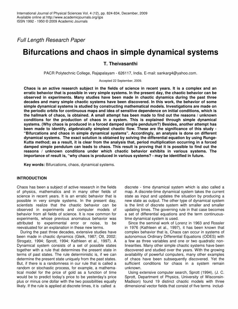
For the map f(x) = 2x (1-x), the fixed points are found by solving the equation x = 2x (1-x). There are two solutions, x = 0 and x = 0.5 which are two fixed points of f(x). The x = y line cuts the function graph at the fixed points. The orbit of the function with initial value 0.1 was drawn. The orbit converges to the sink at x = 0.5. The fixed points are found in the same manner for the map f(x) = (3x-x3) / 2. The map has 3 fixed points namely, -1, 0 and 1. The x = y line cuts the function graph at the fixed points.

The orbits with initial values x = 1.6 and 1.8 are drawn.

Theivasanthi 827

Figure 4. Cobweb plot f(x)=(3x-x3 ) / 2.

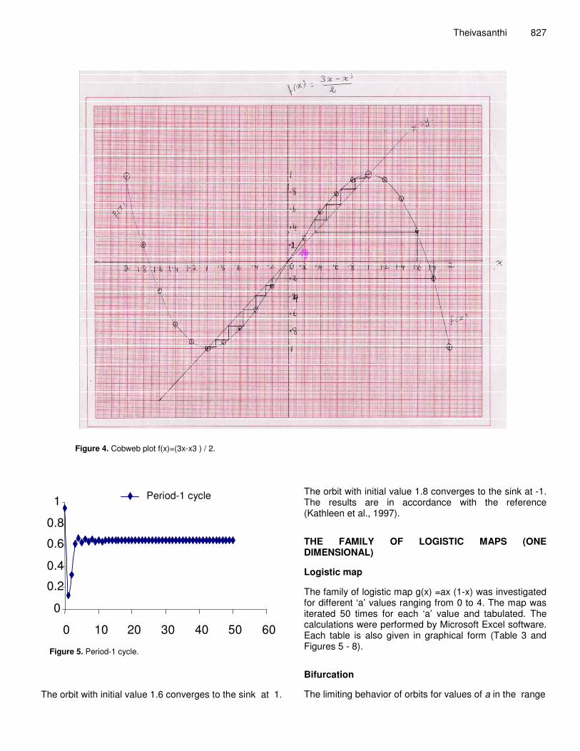
Period-1 cycle

0 0.2 0.4 0.6 0.8

1

0 10 20 30 40 50 60

Figure 5. Period-1 cycle.

The orbit with initial value 1.6 converges to the sink at 1.

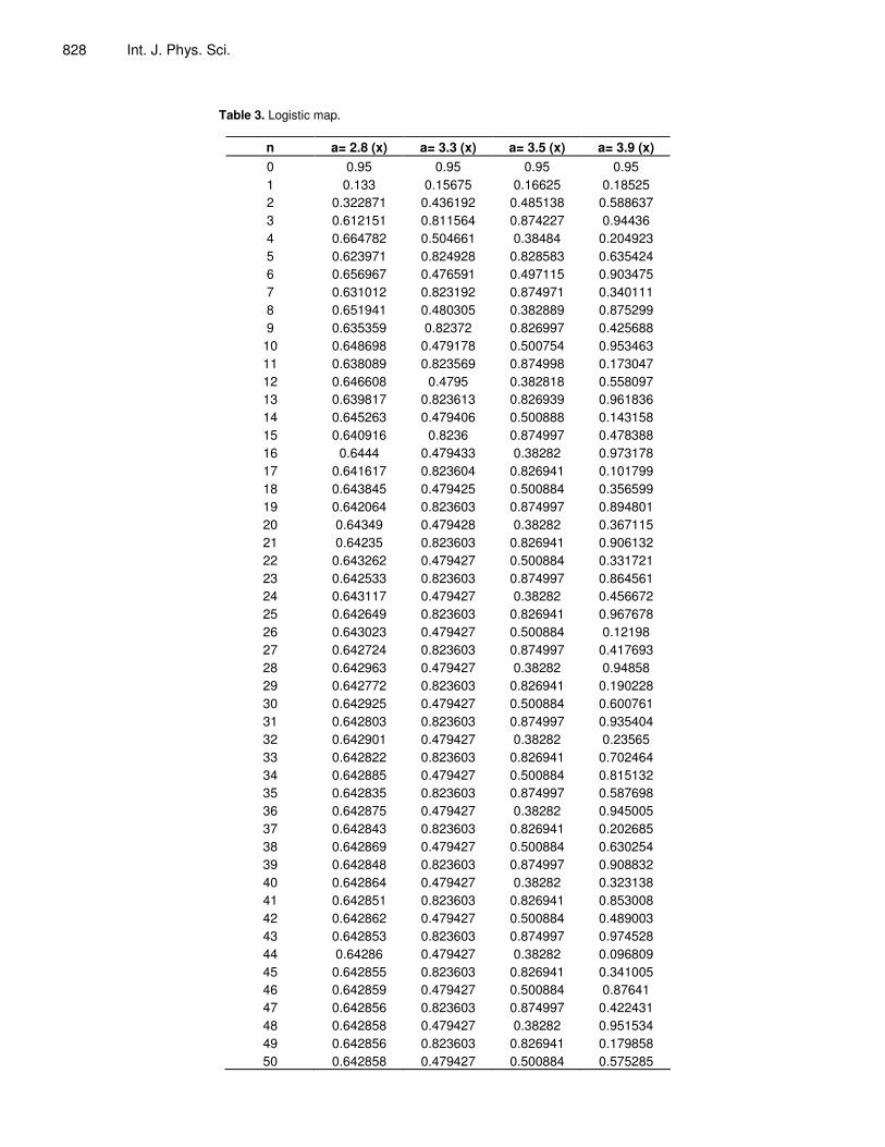
The orbit with initial value 1.8 converges to the sink at -1. The results are in accordance with the reference (Kathleen et al., 1997). THE FAMILY OF LOGISTIC MAPS (ONE DIMENSIONAL) Logistic map The family of logistic map g(x) =ax (1-x) was investigated for different ‘a’ values ranging from 0 to 4. The map was iterated 50 times for each ‘a’ value and tabulated. The calculations were performed by Microsoft Excel software. Each table is also given in graphical form (Table 3 and Figures 5 - 8). Bifurcation The limiting behavior of orbits for values of a in the range

828 Int. J. Phys. Sci.

Table 3. Logistic map.

n a= 2.8 (x) a= 3.3 (x) a= 3.5 (x) a= 3.9 (x) 0 0.95 0.95 0.95 0.95 1 0.133 0.15675 0.16625 0.18525 2 0.322871 0.436192 0.485138 0.588637 3 0.612151 0.811564 0.874227 0.94436 4 0.664782 0.504661 0.38484 0.204923 5 0.623971 0.824928 0.828583 0.635424 6 0.656967 0.476591 0.497115 0.903475 7 0.631012 0.823192 0.874971 0.340111 8 0.651941 0.480305 0.382889 0.875299 9 0.635359 0.82372 0.826997 0.425688

10 0.648698 0.479178 0.500754 0.953463 11 0.638089 0.823569 0.874998 0.173047 12 0.646608 0.4795 0.382818 0.558097 13 0.639817 0.823613 0.826939 0.961836 14 0.645263 0.479406 0.500888 0.143158 15 0.640916 0.8236 0.874997 0.478388 16 0.6444 0.479433 0.38282 0.973178 17 0.641617 0.823604 0.826941 0.101799 18 0.643845 0.479425 0.500884 0.356599 19 0.642064 0.823603 0.874997 0.894801 20 0.64349 0.479428 0.38282 0.367115 21 0.64235 0.823603 0.826941 0.906132 22 0.643262 0.479427 0.500884 0.331721 23 0.642533 0.823603 0.874997 0.864561 24 0.643117 0.479427 0.38282 0.456672 25 0.642649 0.823603 0.826941 0.967678 26 0.643023 0.479427 0.500884 0.12198 27 0.642724 0.823603 0.874997 0.417693 28 0.642963 0.479427 0.38282 0.94858 29 0.642772 0.823603 0.826941 0.190228 30 0.642925 0.479427 0.500884 0.600761 31 0.642803 0.823603 0.874997 0.935404 32 0.642901 0.479427 0.38282 0.23565 33 0.642822 0.823603 0.826941 0.702464 34 0.642885 0.479427 0.500884 0.815132 35 0.642835 0.823603 0.874997 0.587698 36 0.642875 0.479427 0.38282 0.945005 37 0.642843 0.823603 0.826941 0.202685 38 0.642869 0.479427 0.500884 0.630254 39 0.642848 0.823603 0.874997 0.908832 40 0.642864 0.479427 0.38282 0.323138 41 0.642851 0.823603 0.826941 0.853008 42 0.642862 0.479427 0.500884 0.489003 43 0.642853 0.823603 0.874997 0.974528 44 0.64286 0.479427 0.38282 0.096809 45 0.642855 0.823603 0.826941 0.341005 46 0.642859 0.479427 0.500884 0.87641 47 0.642856 0.823603 0.874997 0.422431 48 0.642858 0.479427 0.38282 0.951534 49 0.642856 0.823603 0.826941 0.179858 50 0.642858 0.479427 0.500884 0.575285

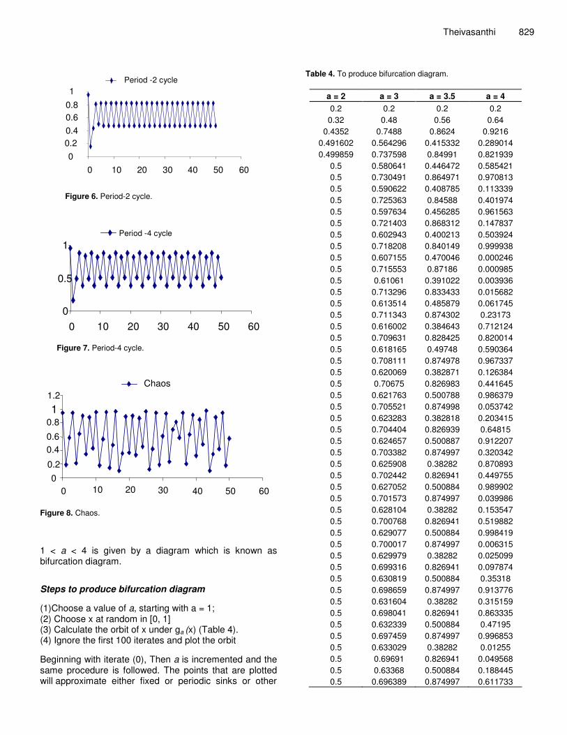
Period -2 cycle

0 0.2 0.4 0.6 0.8 1

0 10 20 30 40 50 60

Figure 6. Period-2 cycle.

0

0.5

1

0 10 20 30 40 50 60

Period -4 cycle

Figure 7. Period-4 cycle.

0 0.2 0.4 0.6 0.8 1

1.2

0 10 20 30 40 50 60

Chaos

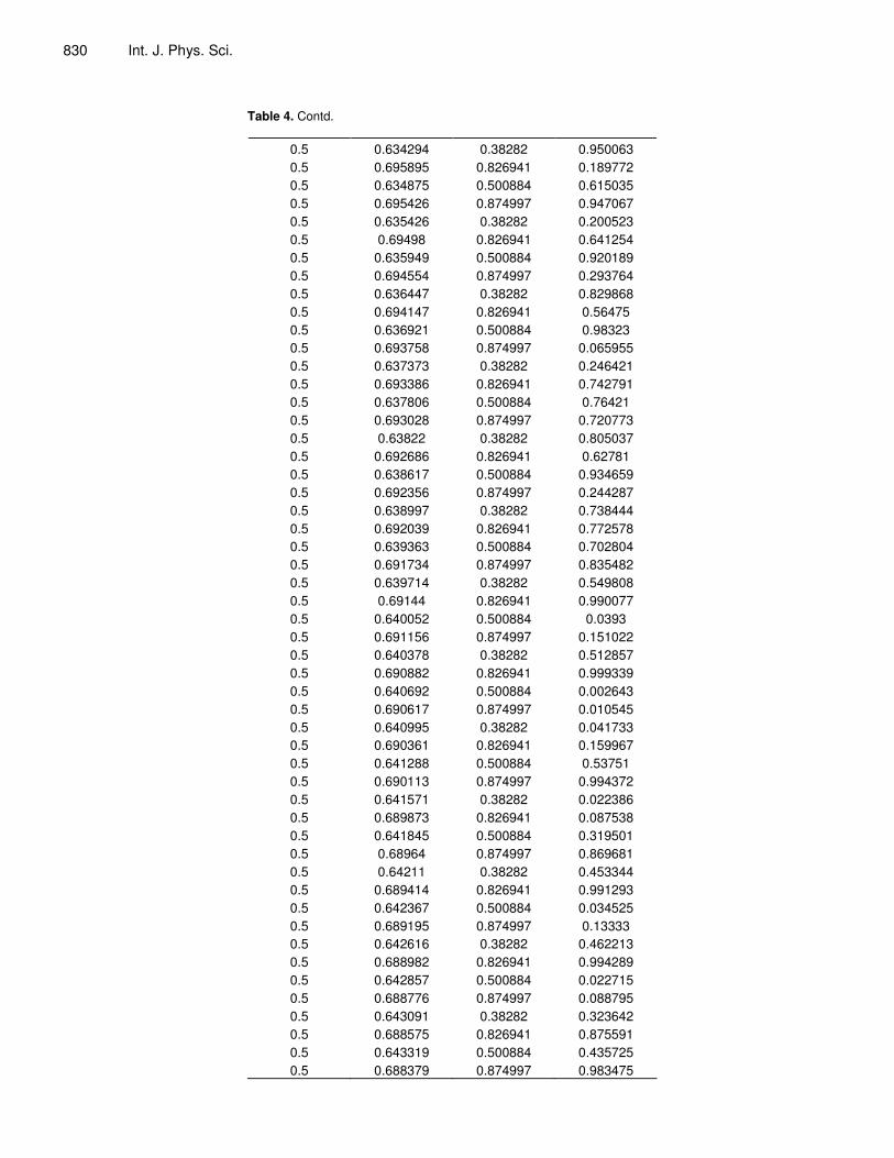
Figure 8. Chaos. 1 < a < 4 is given by a diagram which is known as bifurcation diagram. Steps to produce bifurcation diagram (1)Choose a value of a, starting with a = 1; (2) Choose x at random in [0, 1] (3) Calculate the orbit of x under ga (x) (Table 4). (4) Ignore the first 100 iterates and plot the orbit Beginning with iterate (0), Then a is incremented and the same procedure is followed. The points that are plotted will approximate either fixed or periodic sinks or other

Theivasanthi 829

Table 4. To produce bifurcation diagram.

a = 2 a = 3 a = 3.5 a = 4 0.2 0.2 0.2 0.2

0.32 0.48 0.56 0.64 0.4352 0.7488 0.8624 0.9216

0.491602 0.564296 0.415332 0.289014 0.499859 0.737598 0.84991 0.821939

0.5 0.580641 0.446472 0.585421 0.5 0.730491 0.864971 0.970813 0.5 0.590622 0.408785 0.113339 0.5 0.725363 0.84588 0.401974 0.5 0.597634 0.456285 0.961563 0.5 0.721403 0.868312 0.147837 0.5 0.602943 0.400213 0.503924 0.5 0.718208 0.840149 0.999938 0.5 0.607155 0.470046 0.000246 0.5 0.715553 0.87186 0.000985 0.5 0.61061 0.391022 0.003936 0.5 0.713296 0.833433 0.015682 0.5 0.613514 0.485879 0.061745 0.5 0.711343 0.874302 0.23173 0.5 0.616002 0.384643 0.712124 0.5 0.709631 0.828425 0.820014 0.5 0.618165 0.49748 0.590364 0.5 0.708111 0.874978 0.967337 0.5 0.620069 0.382871 0.126384 0.5 0.70675 0.826983 0.441645 0.5 0.621763 0.500788 0.986379 0.5 0.705521 0.874998 0.053742 0.5 0.623283 0.382818 0.203415 0.5 0.704404 0.826939 0.64815 0.5 0.624657 0.500887 0.912207 0.5 0.703382 0.874997 0.320342 0.5 0.625908 0.38282 0.870893 0.5 0.702442 0.826941 0.449755 0.5 0.627052 0.500884 0.989902 0.5 0.701573 0.874997 0.039986 0.5 0.628104 0.38282 0.153547 0.5 0.700768 0.826941 0.519882 0.5 0.629077 0.500884 0.998419 0.5 0.700017 0.874997 0.006315 0.5 0.629979 0.38282 0.025099 0.5 0.699316 0.826941 0.097874 0.5 0.630819 0.500884 0.35318 0.5 0.698659 0.874997 0.913776 0.5 0.631604 0.38282 0.315159 0.5 0.698041 0.826941 0.863335 0.5 0.632339 0.500884 0.47195 0.5 0.697459 0.874997 0.996853 0.5 0.633029 0.38282 0.01255 0.5 0.69691 0.826941 0.049568 0.5 0.63368 0.500884 0.188445 0.5 0.696389 0.874997 0.611733

830 Int. J. Phys. Sci.

Table 4. Contd.

0.5 0.634294 0.38282 0.950063 0.5 0.695895 0.826941 0.189772 0.5 0.634875 0.500884 0.615035 0.5 0.695426 0.874997 0.947067 0.5 0.635426 0.38282 0.200523 0.5 0.69498 0.826941 0.641254 0.5 0.635949 0.500884 0.920189 0.5 0.694554 0.874997 0.293764 0.5 0.636447 0.38282 0.829868 0.5 0.694147 0.826941 0.56475 0.5 0.636921 0.500884 0.98323 0.5 0.693758 0.874997 0.065955 0.5 0.637373 0.38282 0.246421 0.5 0.693386 0.826941 0.742791 0.5 0.637806 0.500884 0.76421 0.5 0.693028 0.874997 0.720773 0.5 0.63822 0.38282 0.805037 0.5 0.692686 0.826941 0.62781 0.5 0.638617 0.500884 0.934659 0.5 0.692356 0.874997 0.244287 0.5 0.638997 0.38282 0.738444 0.5 0.692039 0.826941 0.772578 0.5 0.639363 0.500884 0.702804 0.5 0.691734 0.874997 0.835482 0.5 0.639714 0.38282 0.549808 0.5 0.69144 0.826941 0.990077 0.5 0.640052 0.500884 0.0393 0.5 0.691156 0.874997 0.151022 0.5 0.640378 0.38282 0.512857 0.5 0.690882 0.826941 0.999339 0.5 0.640692 0.500884 0.002643 0.5 0.690617 0.874997 0.010545 0.5 0.640995 0.38282 0.041733 0.5 0.690361 0.826941 0.159967 0.5 0.641288 0.500884 0.53751 0.5 0.690113 0.874997 0.994372 0.5 0.641571 0.38282 0.022386 0.5 0.689873 0.826941 0.087538 0.5 0.641845 0.500884 0.319501 0.5 0.68964 0.874997 0.869681 0.5 0.64211 0.38282 0.453344 0.5 0.689414 0.826941 0.991293 0.5 0.642367 0.500884 0.034525 0.5 0.689195 0.874997 0.13333 0.5 0.642616 0.38282 0.462213 0.5 0.688982 0.826941 0.994289 0.5 0.642857 0.500884 0.022715 0.5 0.688776 0.874997 0.088795 0.5 0.643091 0.38282 0.323642 0.5 0.688575 0.826941 0.875591 0.5 0.643319 0.500884 0.435725 0.5 0.688379 0.874997 0.983475

Theivasanthi 831

Table 4. Contd.

0.5 0.64354 0.38282 0.065008 0.5 0.688189 0.826941 0.243127 0.5 0.643755 0.500884 0.736064

Table 5. 101st Iterate value.

a 2 3 3 3.5 3.5 3.5 3.5 4 4 4 4 4 4 4 4 x 0.5 0.69 0.64 0.83 0.5 0.87 0.38 0.88 0.44 0.98 0.07 0.24 0.74 0.77 0.69

Bifurcation

Figure 9. Bifurcation.

attracting sets.

The Bifurcation diagram shows the birth, evolution and death of attracting sets. The 101st iterate value for each ‘a’ value is given in Table 5 to draw the bifurcation diagram. The calculations were performed by using Microsoft Excel software.

When 0 < a < 1, the map has a sink at x = 0 and every initial condition between 0 and 1 is attracted to this sink. In other words, with small reproduction rates, small populations tend to die out. If 1 < a < 3, the map has a sink at x = (a-1)/a. Small proportions grow to a steady state of x = (a-1)/a for a > 3, the fixed point is unstable and a period two sink takes its place for a = 3.3. When a grows above 1+�6 � 3.45, the period two sink also becomes unstable. Many new periodic orbits come into existence as a is increased from 3.45 to 4 (Table 5 and Figure 9). TWO DIMENSIONAL MAPS Much of the Chaotic Phenomena present in differential equations can be approached through reduction by time; T maps and Poincare maps. Poincare maps of differential equations can be found as well in a two dimensional quadratic map which is much easier to simulate on a

computer. One such map is the Henon map which is given as f(x, y) = (a - x2 + by, x).

The map has two inputs x, y and two outputs, the new x, y. The new y is just the old x but the new x is a non linear function of the old x and y. The letters a and b represent parameters that are held fixed as the map is iterated. Henon’s remarkable discovery is “barely non-linear” map. It displays an impressive breadth of complex phenomena. In its way, the Henon map is to two dimensional dynamics while the logistic map G(x) = 4x (1-x) is to one dimensional dynamics and it continues to be a catalyst for deeper understanding of nonlinear systems. Along with the sink and source, a new type of fixed point is there, which cannot occur in a one dimensional state space. This type of fixed point which is called as a saddle has at least one attracting direction and at least one repelling direction. For instance, Let A be a linear map. A is hyperbolic if A has no eigenvalues of absolute value one. If a hyperbolic map A has at least one eigenvalue of absolute value greater than one and at least one eigen-value of absolute value smaller than one, then the origin is called a saddle.

There are three types of hyperbolic maps: 1.) One for which the origin is a sink; 2.) One for which the origin is a source; 3.) One for which the origin is a saddle. Hyper-bolic linear maps are important objects of study because they have well defined expanding and contracting directions. Henon map Henon map is given by fa,b = (a - x2 + by, x). Assuming a = 0; b = 0.4; to find the fixed points: -x2 + by = x; -x2 + 0.4x = x; x2 + 0.6x = 0; x(x + 0.6) = 0; x = 0; x = -0.6. Therefore, the fixed points are (0, 0) and (-0.6, -0.6). To check for the fixed point (0, 0): The Jacobian matrix is

D f (x, y) =

-2x b 1 0

832 Int. J. Phys. Sci.

D f (0, 0) =

0 0.4 1 0

-� 0.4 1 0-�

�

2 – 0.4 = 0; �2 = 0.4; � = ± �0.4 = ± 0.632 The eigenvalues are +0.632 and -0.632. Both are less than 1. So the fixed point (0, 0) is a sink.

To check for the fixed point (-0.6, -0.6). The Jacobian matrix is

D f (x, y) =

D f (-0.6, -0.6) =

= -1.2 � + �2 = 0.4

�2 - 1.2 � - 0.4 = 0

� = 1.2 ± � 1.44 + 1.6

2

-2x b 1 0

1.2 0.4 1 0

1.2-� 0.4 1 -�

Eigenvalues equals; 1.472, -0.271. One is greater than one and the other is less than one. So, the fixed point (-0.6, -0.6) is a saddle point. For b = 0.4 and a >0.85, the attractors of the Henon map become more complex (Table 6). When the period two orbits becomes unsta-ble, it is replaced with an attracting period 4 orbit, then a period eight orbit etc.

After 500 iterations, the Henon map displays a single attracting orbit for a particular value of the parameter ‘a’. From the Table 6, we see that for b = 0.4 and a > 0.85,

the attractors of the Henon map become more complex. When a = 0.9, there is a period 4 sink. When a = 0.988, there is an attracting period 16 sink and when a = 1.0293, there is a period 10 sink. Thus, the periodic points are the key to many of the properties of a map (Kathleen et al., 1997). Simple dynamical models In this chapter, we modeled two physical processes with maps. One of the most important uses of maps in scien-tific applications is to assist in the study of a differential equation model. A map describes the time evolution of a system by expressing its state as a function of its previous state. Instead of expressing the current state as a function of the previous state, a differential equation expresses the rate of change of the current state as a function of the current state.

A simple illustration of this type of dependence is Newton’s law of cooling. Consider the state x consisting of the difference between the temperature of a warm object and the temperature of its surroundings. The rate of change of this temperature difference is negatively proportional to the temperature difference itself: x = ax, where a < 0.

The solution of this equation is x (t) = x (0)eat, meaning that the temperature difference x decays exponentially in time. This is a linear differential equation, since the terms involving the state x and its derivatives are linear terms. Since it is a linear differential equation, whatever be the initial condition x (0), there are no attracting fixed points. Another familiar example, which yields a nonlinear differential equation, is that of a pendulum. The pendulum bob hangs from a pivot, which constrains it to move along a circle. The acceleration of the pendulum bob in the tangential direction is proportional to the component of the gravitational downward force in the tangential direction, which in turn depends on the current position of the pendulum. This relation of the second derivative of the angular position with the angular position itself is one of the most fundamental equations in science. The pendulum is an example of a nonlinear oscillator. Other nonlinear oscillators that satisfy the same general type of differential equation include electric circuits and feedback systems. Newton’s law of motion F = ma is used to find the pendulum equation. If L is the length of the pendulum and � is the angle of the pendulum and m is the mass of the pendulum, then the component of acceleration tangent to the circle is L�, because the component of position tangent to the circle is L�. The component of force along the direction of motion is mgsin�. It is a restoring force, meaning that it is directed in the opposite direction from the displacement of the variable �. If the first and second time derivatives of � are � and �, the differential equation governing the frictionless pendulum is mL� = -mgsin�, according to Newton’s law of motion. To simplify, a pendulum of length L = g is use. The equa-

Theivasanthi 833

Table 6. Henon map.

Period 1 Period 2 Period 4 a = 1.2 b = -0.3 a =1.28 b = -0.3 a = 0.9 b = 0.4

x y x y x y 0.623774 0.623774 0.532437 0.766773 -0.23842 0.932101 0.623774 0.623774 0.766478 0.532437 1.215997 -0.23842 0.623774 0.623774 0.53278 0.766478 -0.67402 1.215997 0.623774 0.623774 0.766202 0.53278 0.932101 -0.67402 0.623774 0.623774 0.5331 0.766202 -0.23842 0.932101 0.623774 0.623774 0.765944 0.5331 1.215997 -0.23842 0.623774 0.623774 0.5334 0.765944 -0.67402 1.215997 0.623774 0.623774 0.765701 0.5334 0.932101 -0.67402

-0.23842 0.932101 1.215997 -0.23842 -0.67402 1.215997 0.932101 -0.67402

Period 10 Period 16 a =1.0293 b = 0.4 a = 0.988 b = 0.4

x y x y -0.75447 1.252643 -0.02265 0.82423 0.961137 -0.75447 1.317179 -0.02265 -0.19627 0.961137 -0.75602 1.317179 1.375232 -0.19627 0.943303 -0.75602 -0.94047 1.375232 -0.20423 0.943303 0.694904 -0.94047 1.323612 -0.20423 0.170219 0.694904 -0.84564 1.323612 1.278287 0.170219 0.802338 -0.84564 -0.53663 1.278287 0.005997 0.802338 1.252643 -0.53663 1.308899 0.005997 -0.75447 1.252643 -0.72282 1.308899 0.961138 -0.75447 0.989093 -0.72282 -0.19627 0.961138 -0.27943 0.989093 1.375232 -0.19627 1.035555 -0.27943 -0.94047 1.375232 -0.82825 1.035555 0.694904 -0.94047 0.82423 -0.82825 0.170219 0.694904 -0.02265 0.82423 1.278287 0.170219 1.317179 -0.02265 -0.53663 1.278287 -0.75602 1.317179 1.252643 -0.53663 0.943302 -0.75602 -0.75447 1.252643 0.961138 -0.75447 -0.19627 0.961138 1.375232 -0.19627

tion becomes � = - sin � and the resulting solution is given in Table 7.

Again, there are no fixed points for this nonlinear, two dimensional map. If the damping term -c � is added; corresponding to friction at the pivot, and a periodic term r sin t which is an external force constantly providing energy to the pendulum, the resulting equation becomes

the forced damped pendulum model given as; � = -c� - sin � + r sin t.

An approximate solution for this equation is found for c = 0.2 and r = 1.66. With the initial condition � = 0.3 and � = 0.7, From Table 8, it can be infer that periodic orbits exist (Figure 10).

It is clear from the above discussion that, period multi-

834 Int. J. Phys. Sci.

Table 7. Undamped simple pendulum.

� � 0.3 0.7

0.29552 0.755336 0.291238 0.756651 0.287138 0.757889 0.283208 0.759058 0.279438 0.760164 0.275815 0.761211 0.272331 0.762204 0.268978 0.763146 0.265746 0.764043

Table 8. Damped simple pendulum.

� � 1.136717 -0.28691 0.124961 0.220575 -1.631522 0.792203 1.097059 -0.260688 0.034552 0.256215 -1.657816 0.799403 1.136717 -0.28691 0.124961 0.220575 -1.631522 0.792203 1.097059 -0.260688 0.034552 0.256215 -1.657816 0.799403 1.136717 -0.28691 0.124961 0.220575 1.631522 0.792203 1.097059 -0.260688 0.034552 0.256215 -1.657816 0.799403 1.136717 -0.28691 0.124961 0.220575 -1.631522 0.792203 1.097059 -0.260688 0.034552 0.256215 -1.657816 0.799403

-0.4-0.2

00.2 0.4 0.6 0.8

1

-2 -1 0 1 2

Figure 10. Attractors for forced damped pendulum.

plication occurs for forced damped simple pendulum which leads to chaotic solution. The exact solution can be obtained by solving the differential equation by using Runge-kutta method. Thus, an analysis is done on different dynamical systems and the condition under which bifurcation and chaos occur in such systems. ACKNOWLEDGEMENTS The author expresses immense thanks to Mrs. S. Sivadevi (Lecturer in Physics), The SFR College for Women, Sivakasi, India for valuable suggestions and encouragement. REFERENCES Gleik J (1987). Chaos: Making a New Science (Penguin Books, New

York). Kathleen TA, Tim DS, James A (1997). Yorke – Chaos- An introduction

to dynamical systems, Springer-verlag New York. Ott E (2002). Chaos in Dynamical Systems. Sprott JC (1994). Phys. Rev. E 50-R 647. Strogatz SH (1994). Nonlinear Dynamics and Chaos (Addia-Wesley,

Reading). Vinod P, Sud KK (2005). Bifurcation and Chaos in Simple jerk

Dynamical systems, Pramana, January, 64: 75-93. Vinod P, Sud KK (2006). Identical synchronization in chaotic jerk

dynamical Systems, Electronic J. Theor. Phys. 3(11): 33 – 70.