arX

iv:q

uant

-ph/

0505

085v

1 1

1 M

ay 2

005

CHAOS AND QUANTUM MECHANICS

Salman HabibMS B285, Theoretical Division, The University of California, Los Alamos National Laboratory,Los Alamos, New Mexico 87545

habib@lanl.gov

Tanmoy Bhattacharya,1 Benjamin Greenbaum,2 Kurt Jacobs,1,3

Kosuke Shizume,4 and Bala Sundaram,5

1Los Alamos National Laboratory,2Columbia University,3Griffith University,4Tsukuba Uni-versity,5City University of New York

AbstractThe relationship between chaos and quantum mechanics has been somewhat

uneasy – even stormy, in the minds of some people. However, much of theconfusion may stem from inappropriate comparisons using formal analyses. Incontrast, our starting point here is that a complete dynamical description requiresa full understanding of the evolution ofmeasured systems, necessary to explainactual experimental results. This is of course true, both classically and quantummechanically. Because the evolution of the physical state is now conditionedon measurement results, the dynamics of such systems is intrinsically nonlineareven at the level of distribution functions. Due to this feature, the physicallymore complete treatment reveals the existence of dynamicalregimes – such aschaos – that have no direct counterpart in the linear (unobserved) case. More-over, this treatment allows for understanding how an effective classical behaviorcan result from the dynamics of an observed quantum system, both at the level oftrajectories as well as distribution functions. Finally, we have the striking predic-tion that time-series from measured quantum systems can be chaotic far from theclassical regime, with Lyapunov exponents differing from their classical values.These predictions can be tested in next-generation experiments.

1. Prologue

I met Henry Kandrup as a graduate student at Maryland in 1985,havingrecently decided to switch from experiment to theory. My first interactionwith postdocs – at the time an intimidatingly higher form of life – occurredwhen Henry suggested that he and another postdoc, Ping Yip, and I take up the

2

question of Landau damping and stability of star clusters. While I was happyto work with Henry and Ping, most of the time I was struggling to understandcryptic conversations laced with mathematical jargon – “functions of compactsupport,” “consider the following inner product,” and so on. Since I wasn’tfollowing too much of this, I decided it was better to go away and catch up byreading every paper that was even vaguely related to the topic. This turned outto be much easier than expected, and one night I came up with a simple wayof combining Henry’s previous work on stability with conventional Landaudamping theory from plasma physics. Coming in to the department late in themorning I showed the first set of notes to Henry. He looked at them, did notsay much – which was unusual – and went back home. Next day, as Ienteredmy office, I was stunned to find, slipped under the door, a complete preprint ofa paper, all equations written in by hand in Henry’s beautiful copperplate. Hehad gone home, generalized my notes to the problem at hand, worked throughthe entire thing, come back late at night, and typed the preprint on an electrictypewriter (this was just before the advent of word processing), finishing as thesun came up. After this incident, I wasreally afraid of postdocs!

My early interactions with Henry were very wide-ranging; wediscussed allsorts of topics, from classical statistical mechanics to quantum gravity, and onall of them he was very well-informed and entertainingly opinionated. Theyears went by quickly, Henry moved on to other places and so did I. Althoughwe argued and collaborated now and then as of old, in my memorythe earlyyears have a certain luminescence. My favorite remembranceof Henry is thatafter he had demolished somebody’s hapless piece of research in one of ourdiscussions, he would look up, smile in a disarming way, and say, “True?” Itusually was.

One of the topics Henry and I discussed at considerable length and depthwas the nature of chaos in multi-particle systems and its role in controllingaspects of the dynamical behavior of statistical averages.While we did notalways agree, these discussions certainly attuned my thinking about the prob-lem. In this contribution, I present a discussion of how to think about chaos in aphysical way, from the point of view of realistic experiments. The basis of thearguments applies to both classical and quantum systems andserves to bringtogether these two great dynamical traditions that are seemingly at such oddswith each other. The work reported here is the result of several collaborationsbetween subsets of the authors. While I do not know what Henry’s opinionswould have been on this subject, however, I am sure he would not have beenquiet!

Chaos and Quantum Mechanics 3

2. Introduction

In classical theory – unlike in quantum mechanics – the status of dynamicalchaos is apparently clear: chaos exists observationally and is well-describedtheoretically by Newton’s equations. (Nevertheless, evenhere, a deeper look atthe physical meaning of chaos is certainly helpful; we return to this presently.)It is in the context of quantum theory, however, that the notion of chaos appearsso puzzling and mysterious. Because of the Kosloff-Rice theorem [1] and re-lated results [2], it is clear that quantum evolution of the wave function or thedensity matrix is integrable; hence, chaos cannot exist in quantum mechanicsin the canonical sense. This is the basic stumbling block to defining a quantumnotion of nonintegrability.

One may argue that real quantum systems are always coupled toan envi-ronment and hence their evolution – “for all practical purposes,” (FAPP), inBell’s famous phrase [3] – should be described by unitarity-breaking masterequations rather than the unitary evolution assumed by the Kosloff-Rice theo-rem. Perhaps this way out, although not fundamentally satisfying to the purist,is enough by itself, but it is easy to see what is wrong with theargument.Fundamentally, any fully quantum dynamical description must arise from aHamiltonian describing the system, its environment, and their coupling. Themaster equation represents the evolution of the reduced density matrix for thesystem which arises from tracing over the environment variables in the full(system plus environment) density matrix. Since the full evolution must satisfyKosloff-Rice, the evolution of the reduced density matrix cannot be noninte-grable.

Thus, the fundamental problem we are faced with is this: we are familiarwith chaos in the real world, but our fundamental theory of dynamics – whichpasses every experimental test beautifully – seemingly does not have a naturalplace within it to tolerate even the existence of the concept. This should notcome as a surprise; after all, the trajectories of classicalmechanics are appar-ently “real” and effortless to contemplate, but they too, have no natural placein quantum mechanics. Now it is true that quantum mechanics is an intrin-sically probabilistic theory, but that, in itself, is not the real issue. Classicaltheory can be easily cast as fundamentally probabilistic aswell, via the clas-sical Liouville equation describing the evolution of a classical probability inphase space. (For an attempt at an even closer analogy, see Ref. [4] and thediscussion in Ref. [5].) As discussed further below, the keypoint is rather that,unlike special relativity, wherev/c → 0 smoothly transitions between Einsteinand Newton, the limit̄h → 0 is singular. The symmetries underlying quantumand classical dynamics – unitarity and symplecticity, respectively – are funda-mentally incompatible with the opposing theory’s notion ofa physical state:

4

quantum-mechanically, a positive semidefinite density matrix; classically, apositive phase-space distribution function.

In the rest of this article, we will expose the singular nature of theh̄ → 0limit and discuss a physical point of view – applicable to both classical andquantum systems – which will enable us to explain how trajectories and chaosappear in real experiments.

At this point, it should be clear that the questions taken up in this contribu-tion are not those usually considered under the research area called “quantumchaos.” There, one is primarily interested in the quantum behavior of a systemwith a classically chaotic Hamiltonian, what might happen to the validity ofcertain approximations (e.g., semiclassical approaches to calculating the quan-tum propagator) and whether classical trajectories and phase space structurescan provide some insight into the nature of quantum wavefunctions. But onedoes not actually study quantum chaos.

We distinguish betweenisolatedevolution, where the system state evolveswithout any coupling to the external world,unconditioned openevolution,where the system evolves coupled to an external environmentbut where noinformation regarding the system is extracted from the environment, andcon-ditioned openevolution where such informationis extracted. In the third case,the evolution of the physical state is driven by the system evolution, the cou-pling to the external world, and by the fact that observational information re-garding the state has been obtained. This last aspect – system evolutioncondi-tionedon the measurement results via Bayesian inference – leads toan intrinsi-cally nonlinear evolution for the system state, and distinguishes it from uncon-ditioned evolution. While the concept of conditioned evolution of the systemstate is familiar to engineers and mathematicians, especially systems engineersand control theorists [6], it is not yet completely familiarterritory to the major-ity of physicists. Nevertheless, driven by the impressive progress in the exper-imental state-of-the-art in quantum and atomic optics and in nanoscience [7],these notions are now being employed as everyday tools at least in some fields.

The conditioned evolution provides, in principle, the mostrealistic possibledescription of an experiment. To the extent that quantum andclassical mechan-ics are eventually just methodological tools to explain andpredict the resultsof experiments, this is the proper context in which to compare them and dis-cuss the nature of predictions for real experiments. The explicit incorporationof information gained via measurement also provides a structure to addressthe quantum-classical transition more generally, and to frame the question ofwhere chaos exists within this structure.

The fact that quantum and classical mechanics are fundamentally incompat-ible in many ways, yet the macroscopic world is well-described by classicaldynamics has puzzled physicists ever since the laying of thefoundations of

Chaos and Quantum Mechanics 5

quantum theory. It is fair to say that not everyone is satisfied with the state ofaffairs – including many seasoned practitioners of quantummechanics.

Of course, the notion of measurement in quantum mechanics – the denial ofreality to system properties unless they are measured – is such a revolutionaryconcept that it engenders much more unease [8], even today. The problem isthat, were quantum mechanics the final theory, it could deny reality to the mea-surement results themselves unless they were observed by another system andso on,ad infinitum. In order to “solve” the “measurement problem,” it orig-inally appeared impossible to think of quantum mechanics asa fundamentaltheory without relying on the existence of a classical world-view within whichto embed it [9]. Although we still cannot dispel the unease invoked by the mea-surement problem, it is important to stress that the quantum-classical transitioncan be understood independently. This transition should not be confused withthe measurement problem.

A partial understanding of the classical limit arises from the idea – familiarfrom nonequilibrium statistical mechanics – that weak interactions of a sys-tem with an environment are universal [10]. These interactions can effectivelysuppress certain nonclassical terms in the quantum evolution [11]. However,at best they only allow for the emergence of a classical probabilistic evolutionand it can be shown that the mere existence of such interactions is insufficientto yield classical evolution in all cases [12]. Finally, this picture alone cannotexplain the results of actual measurements where information can be continu-ously extracted from the environment and used to define operational notions ofa trajectory. We now go in to these questions in more detail.

3. Isolated and Open Evolution

Suppose we are given an arbitrary system HamiltonianH(x, p) in termsof the dynamical variablesx andp; we will be more specific regarding theprecise meaning ofx andp as position and momentum later. The Hamilto-nian is the generator of time evolution for the physical system state, providedthere is no coupling to an environment or measurement device. In the classicalcase, we specify the initial state by a positive phase space distribution func-tion fCl(x, p); in the quantum case, by the (position-representation) positivesemidefinite density matrixρ(x1, x2) or, completely equivalently, by the cor-responding Wigner distribution functionfW (x, p) (not positive). The Wignerdistribution [13, 14] is a “half-Fourier” transform ofρ(x1, x2), defined as

fW (x, p) =1

2πh̄

∫

d∆ρ(x +1

2∆, x − 1

2∆) exp(−ip∆/h̄), (1)

wherex ≡ (x1 + x2)/2 and∆ ≡ x1 − x2.The evolution of anisolatedsystem is then given by the classical and quan-

tum Liouville equations for thefine-graineddistribution functions (i.e., the

6

evolution is entropy-preserving):

∂tfCl(x, p) = −[

p

m∂x − ∂xV (x)∂p

]

fCl(x, p), (2)

∂tfW (x, p) = −[

p

m∂x − ∂xV (x)∂p

]

fW (x, p)

+∞∑

λ=1

(h̄/2i)2λ

(2λ + 1)!∂2λ+1

x V (x)∂2λ+1p fW (x, p), (3)

where we have assumed for simplicity that the potentialV (x) can be Taylor-expanded; this does not alter the nature of any of the following arguments.Note that these evolutions are both linear in the respectivedistribution func-tions.

The limiting formfCl(x, p) = δ(x− x̄)δ(p− p̄) is allowed classically, and,on substitution in Eqn. (2), yields the expected Newton’s equations. Thesemay then be interpreted as equations for the particle position and momentum,although we must emphasize that this identification is only formal at this stage.Quantum mechanically, this ultralocal limit is not permitted sincefW (x, p)must be square-integrable, therefore – even formally – no direct particle inter-pretation can exist. In both cases, if one allows for initially localized distri-butions but which nevertheless have some finite width, it is easy to see that ifV (x) is nonlinear, quite generically the distribution will eventually spread overthe allowed phase space and not remain localized.

As alluded to in the Introduction, the extension to open systems is concep-tually trivial, but very difficult to implement in practice.To the original systemHamiltonian, we now add pieces representing the environment and the system-environment coupling. If the environment is in principle unobservable, thena (nonlocal in time) linear master equation for the system’sreduced densitymatrix is – in theory – derivable by tracing over the environmental variables.In practice, tractable equations are impossible to obtain without drastic simpli-fying assumptions such as weak coupling, timescale separations, and simpleforms for the environmental and coupling Hamiltonians. In any case, the im-portant point to note is that the act of tracing over the environment does notchange the linear nature of the equations. Generally speaking, master equa-tions describing open evolution ofcoarse-graineddistributions augment theRHS of Eqns. (2) and (3) with terms containing dissipation and diffusion ker-nels connected via generalized fluctuation-dissipation relations [15]. Whilethe classical diffusion term vanishes in the limit of zero temperature for theenvironment, this is not true quantum mechanically due to the presence ofzero-point fluctuations.

Chaos and Quantum Mechanics 7

4. Continuous Measurement and Conditioned Evolution

In contrast to classical theory, where measurement can be, in principle, apassive process, in quantum theory measurement creates an irreducible distur-bance on the observed system (quantum “backaction”). This being so, if ouraim is that measurement yield dynamical information – rather than stronglyinfluence dynamics – the desired measurement process must yield a limitedamount of information in a finite time. Hence, simple projective (von Neu-mann) measurements are clearly not appropriate because they yield completeinformation instantaneously via state projection. Nevertheless, this fundamen-tal notion of measurement can be easily extended [5] to devise schemes thatextract information continuously [16]. The basic idea is tohave the systemof interest interact weakly with another (e.g., atom interacting with an elec-tromagnetic field) and make projective measurements on the auxiliary system(e.g., photon counting). Because of the weak interaction, the state of the aux-iliary system gathers very little information regarding the system of interest,and therefore this system, in turn, is only perturbed slightly by the measure-ment backaction. Only a small component of the information gathered by theprojective measurement of the auxiliary system relates to the system of inter-est, and a continuous limit of the measurement process can betaken.

In the continuous limit, the evolution of the system densitymatrix is fun-damentally different from the equations discussed above for the case of openevolution. The master equation describing the evolution ofthe reduced den-sity matrix conditioned on the results of the measurements contains a term thatreflects the gain in information arising from the measurement record (“inno-vation” in the language of control theory). This term, arising from applyinga continuous analog of Bayes’ theorem, is intrinsically nonlinear in the distri-bution function. The coupling to an external probe (and the associated envi-ronment) will also cause effects very similar to the open evolution consideredearlier, and there can once again be dissipation and diffusion terms in the evo-lution equations. The primary differences between the classical and quantumtreatments, aside from the kinematic constraints on the distribution functions,are the following: (i) the (nonlocal inp) quantum evolution term in Eqn. (3),and (ii) an irreducible diffusion contribution due to quantum backaction re-flecting theactivenature of quantum measurements.

We now consider a simple model of position measurement to provide a mea-sure of concreteness. In this model, we will assume that there are no environ-mental channels aside from those associated with the measurement. Supposewe have a single quantum degree of freedom, position in this case, undergo-ing a weak, ideal continuous measurement [16]. Here “ideal”refers to no lossof information during the measurement, i.e., a fine-grainedevolution with noincrease in entropy. Then, we have two coupled equations, one for the mea-

8

surement recordy(t),

dy = 〈x〉dt +1√8k

dW (4)

wheredy is the infinitesimal change in the output of the measurement devicein time dt, the parameterk characterizes the rate at which the measurementextracts information about the observable, i.e., thestrengthof the measure-ment [17], anddW is the Wiener increment describing driving by Gaussianwhite noise [18], the difference between the actually observed value and thatexpected. The other equation – the nonlinear stochastic master equation (SME)– specifies the resulting conditioned evolution of the system density matrix,given in the Wigner representation,

fW (x, p, t + dt) =

[

1 + dt

[

− p

m∂x + ∂xV (x)∂p + DBA∂2

p

]

+ dt∞∑

λ=1

(h̄/2i)2λ

(2λ + 1)!∂2λ+1

x V (x, t)∂2λ+1p

]

fW (x, p, t)

+dt√

8k(x − 〈x〉)fW (x, p, t)dW, (5)

whereDBA = h̄2k is the diffusion coefficient arising from quantum back-action and the last (nonlinear) term represents the conditioning due to themeasurement. In principle, there is also a (generalized) damping term [19],but if the measurement coupling is weak enough, it can be neglected. If wechoose to average over all the measurement results, which isthe same as ig-noring them, then the conditioning term vanishes, butnot the diffusion fromthe measurement backaction. Thus the resulting linear evolution of the coarse-grained quantum distribution is not the same as the linear fine-grained evolu-tion (3), but yields a conventional open-system master equation. Moreover,for a given (coarse-grained) master equation, different underlying fine-grainedSME’s may exist, specifying different measurement possibilities.

In contrast to the quantum case, the corresponding (ideal) classical condi-tioned master equation [seth̄ = 0 in Eqn. (5), holdingk fixed],

fCl(x, p, t + dt) =

[

1 − dt

[

p

m∂x − ∂xV (x)∂p

]]

fCl(x, p, t)

+dt√

8k(x − 〈x〉)fCl(x, p, t)dW, (6)

does not have the backaction term as these classical measurements arepassive:averaging over all measurements simply gives back the Liouville equation (2),and there is no difference between the fine-grained and coarse-grained evolu-tions in this special case. [In general, classical diffusion terms from ordinaryopen evolution can also coexist, as in thea posteriori evolution specified bythe Kushner-Stratonovich equation [20], of which Eqn. (6) is a special case.]

Chaos and Quantum Mechanics 9

As a final point, we delay our discussion of how the classical trajectory limit isincorporated in Eqn. (6), i.e., the precise sense in which the “the position of aparticle is what a position-detector detects,” to the next section.

5. QCT: The Quantum-Classical Transition

If quantum mechanics is really the fundamental theory of ourworld, then aneffectively classical description of macroscopic systemsmust emerge from it– the so-called quantum-classical transition (QCT). It turns out that this issueis inextricably connected with the question of the physicalmeaning of dynam-ical nonlinearity discussed above. Having written down therelevant evolutionequations, we now analyze two notions of the QCT and how they emerge fromthe equations.

Quantum mechanics is intrinsically probabilistic, but classical theory – asshown above by the existence of the delta-function limit forthe classical dis-tribution function – is not. Since Newton’s equations provide an excellent de-scription of observed classical systems, including chaotic systems, it is crucialto establish how such a localized, or trajectory, description can arise quantummechanically. We will call this thestrong form of the QCT. Of course, inmany situations, only a statistical description is possible even classically, andhere we demand only the agreement of quantum and classical distributions andthe associated dynamical averages. This defines theweakform of the QCT.

It is clear that if the strong form of the QCT holds, then, via trivial coarse-graining, the weak form follows automatically. The reverseis not true, how-ever: results from a coarse-grained analysis cannot be applied to the fine-grained situation. Moreover, the violation of the conditions necessary to es-tablish the strong form of the QCT need not prevent the existence of a weakQCT. We now discuss and establish the conditions under whichthese transi-tions occur. Since the strong form of the QCT requires treating the localizedlimit, a cumulant expansion for the distribution function immediately suggestsitself, whereas, for the more nonlocal issues relevant to the weak form of theQCT, a semiclassical analysis turns out to be natural.

5.1 Strong Form of the QCT: Chaos in the Classical Limit

It is easy to see that the strong form of the QCT is impossible to obtain fromeither the isolated or open evolution equations for the density matrix or Wignerfunction. As mentioned already, for a generic dynamical system, a localizedinitial distribution tends to distribute itself over phasespace – and then continueto evolve – either in complicated ways (isolated system) or asymptote to anequilibrium state (open system), whether classically or quantum mechanically.In the case of conditioned evolution, however, the distribution can be localizeddue to the information gained from the measurement, and evolve in a quite

10

different manner. In order to quantify how this happens, letus first apply acumulant expansion to the (fine-grained) conditioned classical evolution (6).This results in the following equations for the centroids (x̄ ≡ 〈x〉, p̄ ≡ 〈p〉),

dx̄ =p̄

mdt +

√8kCxxdW,

dp̄ = 〈F (x)〉dt +√

8kCxpdW, (7)

where

F (x) = −∂xV (x),

CAB =1

2(〈AB〉 + 〈BA〉 − 2〈A〉〈B〉), (8)

along with a hierarchy of coupled equations for the time-evolution of the highercumulants. These equations are the continuous measurement, real-world, ana-log of the formal ultralocal Newtonian limit of the distribution function in theclassical Liouville equation (2). Whereas Eqns. (7) alwaysapply, our aim isto determine the conditions under which the cumulant expansion effectivelytruncates and brings their solution very close to that of Newton’s equations.This will be true provided the noise terms are small (in an average sense) andthe force term is localized, i.e.,〈F (x)〉 = F (x̄) + · · ·, the corrections beingsmall. The required analysis involves higher cumulants andhas been carriedout elsewhere [21]. It turns out that the distribution is localized provided

8k ≫√

(∂2xF )2|∂xF |2mF 2

(9)

and the motion of the centroid will effectively define a smooth classical trajec-tory – the low-noise condition – as long as

k ≫ 2|∂xF |S

(10)

whereS is the action scale of the system. Note that this condition does notbound the measurement strength: classically we can always extract as muchinformation as needed – at least in principle – to gain the trajectory limit. This,then, is the “realistic” derivation of Newton’s equations.

We now turn to the quantum version of these results. In this case, the anal-ogous cumulant expansion gives exactly the same equations for the centroidsas above, while the equations for the higher cumulants are different. (The evo-lution of classical and quantum averages is the same to Gaussian order, withthe first differences arising at the next order [22].) We can again investigatewhether a trajectory limit exists. Localization holds in the weakly nonlinear

Chaos and Quantum Mechanics 11

case if the classical condition above is satisfied. In the case of strong nonlin-earity, the inequality becomes [21]

8k ≫ (∂2xF )2h̄

4mF 2. (11)

Because of the backaction, the low-noise condition is implemented in the quan-tum case by a double-sided inequality:

2|∂xF |s

≪ h̄k ≪ |∂xF |s4

, (12)

where the action is measured in units ofh̄, s being dimensionless. The leftinequality is the same as the classical one discussed above,however the rightinequality is essentially quantum mechanical. The measurement strength can-not be made arbitrarily large as the backaction will result in too large a noise inthe equations for the centroids. As the actions is made larger, both inequali-ties are satisfied for an ever wider range of values ofk. For sufficiently larges,the actual value ofk becomes irrelevant and the dynamics becomes effectivelyclassical.

To recapitulate, for continuously measured quantum systems, trajectoriesthat emerge in the macroscopic limit follow Newton’s equations, and hencecan be chaotic as shown elsewhere [21]. Thus, as speculated in a prescientpaper by Chirikov [23], measurement indeed provides the missing link between“quantum” and “chaos,” at least in the classical limit.

Finally, in experiments one usually considers the measurement record itselfrather than the estimated state of the system as we have discussed so far. Asmeasurement introduces a white noise, it is important to investigate the con-dition under which the record tracks the estimate faithfully. If ∆t is the timeover which the continuous measurement is averaged to obtainthe record (thisaveraging being a necessary part of any finite-bandwidth experiment), and weallow ourselves a maximum of∆x as the position noise, it is easy to see thatthe measurement strength needs to satisfy [21]

8k >1

∆t(∆x)2(13)

To demonstrate these results for a concrete example, we revisit the resultsof Ref. [21] for a driven, Duffing oscillator, with system Hamiltonian

H = P 2/2m + Bx4 − Ax2 + Λx cos(ωt), (14)

with m = 1, B = 0.5, A = 10, Λ = 10, ω = 6.07. This Hamiltonian has beenused before in studies of quantum chaos [24] and quantum decoherence [25]

12

−5 0 5−15

−10

−5

0

5

10

15

⟨ X⟩

⟨ P

⟩

0 10 20 30 40 500

0.5

1x 10

−5

Vx

t

(b)

(a)

Figure 1. (a) The quantum trajectory in phase space for a continuouslymeasured Duffingoscillator [21], withh̄ = 10−5 andk = 105. (b) The position variance,Vx, as a function oftime. Note the smallness of the scale on the y-axis!

and, in the parameter regime used, a substantial area of the accessible phasespace is stochastic.

Numerical calculations at various values ofh̄ confirm that as̄h is reduced,both the steady-state variance, and the resulting noise (for optimal measure-ment strengths) are reduced, as expected. As the dynamical time scale of thisproblem is1 − 0.1 (in units of the driving period), the continuous observationrecord was averaged over a period of0.01. Similarly, as the range of the mo-tion covers distances ofO(10), we demand that the position be tracked to anaccuracy of0.01 to define an effective “trajectory.” To satisfy this, we needtohavek ∼ O(105) or larger [Cf. Eqn. (13)]. In our example, we choose theenergy to beO(102), the corresponding typical action turns out to beO(10),and the typical nonlinearity makes the RHS of Eqn. 9,O(1). We see that achoice ofh̄ = 10−5 andk = 105, satisfies all the constraints for a classicalmotion. In Fig. 1 we demonstrate that in this regime, localization is maintainedalong with low levels of trajectory noise. Fig. 1(a) shows a typical phase spacetrajectory, with the position variance during the evolution, Vx ≡ (∆x)2, plot-ted in Fig. 1(b). We find that the width∆x is always bounded by3.4 × 10−3.Furthermore, as is immediately evident from the smoothnessof the trajectoryin Fig. 1(a), the noise is also negligible on these scales. Additionally, one canverify that the quantum trajectory evolution and that givenby a classical trajec-

Chaos and Quantum Mechanics 13

tory with an equivalent noise are essentially identical – and chaotic – yieldinga Lyapunov exponent of0.57. We return to discuss the Lyapunov exponentlater below.

5.2 Chaos and the Weak Form of the QCT

The weak form of the QCT utilizes thecoarse-graineddistribution func-tion (averaging over all measurements), whereas the strongform refers to thefine-graineddistribution for a single measurement realization. It is importantto reiterate that nonexistence of the strong form of the QCT does not influencethe existence of the weak form of the QCT: It does not matter ifthe distribu-tion is too wide, as long as the classical and quantum distributions agree, and,even if the backaction noise is large, the coarse-grained distribution can re-main smooth and the weak quantum-classical correspondencestill exist. Con-sequently, this correspondence has to be approached in a different manner. Infact, the weak version is just another way to state the conventional decoherenceidea [11]; however, as discussed elsewhere [12], mere suppression of quantuminterference does not guarantee the QCT even in the weak form.

We now focus on a semiclassical analysis of the weak QCT for bounded,classically chaotic open systems [26]. This analysis is best regarded as aregu-larizationof the singular̄h → 0 limit via the environmental interaction. This isdistinct from the statelocalizationcharacteristic of the strong form of the QCT.Given a small, but finite, value of̄h, the aim is to establish the existence of atimescale beyond which the dynamics of open quantum and classical systemsbecomes statistically equivalent if the environmental interaction is sufficientlystrong.

It has been demonstrated [26] that, for a bounded open systemwith a clas-sically chaotic Hamiltonian, the weak form of the QCT is achieved by twoparallel processes, both relying essentially on the existence of environmentaldiffusion. First, the semiclassical approximation for quantum dynamics, whichbreaks down for classically chaotic systems due to overwhelming nonlocal in-terference, is recovered as the environmental interactionfilters these effects.Second, environmental noise restricts the foliation of theunstable manifold,the set of points which approach a hyperbolic point in reverse time, allowingthe semiclassical wavefunction to track this modified classical geometry. Inthis way, the noise prevents classical chaos from breaking the semiclassicalapproximation as̄h → 0, and thus regularizes this limit. Note that this ap-proach explicitly incorporates both the stretching and folding typical of hyper-bolic regions as well as the role of the environment as a filteron a phase-spacequantum distribution.

We begin with a simple model of a quantum system weakly coupled to theenvironment so as to maintain complete positivity for the subsystem density

14

matrix,ρ(t), while subjecting it to a, time-local, unitarity-breakinginteraction.These conditions mathematically constrain the master equation to be of theso-called Lindblad form [27]. If this environmental interaction couples to theposition, as is often the case, the master equation takes theform:

∂fw

∂t= Lclfw + Lqfw + D

∂2fw

∂p2, (15)

whereLcl, the classical Liouville operator, andLq, the quantum correction, canbe easily identified from Eqn. (3). We note in passing that while the sum ofLcl andLq is clearly unitary, individually the operators are not unitary [12]. Inthis simple master equation, we have neglected the dissipative environmentalchannel and kept the diffusive channel for two reasons: (i) the coupling to theenvironment is always assumed to be weak and the dissipativetimescales are,hence, very long, longer than the dynamical timescales of interest, (ii) the weakform of the QCT arises only from the diffusive channel, hence, dissipativeeffects are not of interest here.

WhenLq = 0, this equation reverts to the classical Fokker-Planck equa-tion. It is important to keep in mind that the specific form of the diffusioncoefficient depends strongly on the physical situation envisaged. Thus, if themaster equation describes a weakly coupled, high temperature environment,D = 2mγkBT (γ is the damping coefficient) [28], whereas for a weak, con-tinuous measurement of position, the diffusion due to quantum backaction isD = h̄2k [16]. The discussion below holds for all of these cases.

Once the QCT occurs, the effects ofLq in the evolution specified by Eqn. (15)are subdominant. Therefore, to understand how environmental noise acts inthis limit, it suffices to consider the behavior of the corresponding classicalFokker-Planck equation. To do this, it is convenient to examine the underly-ing Langevin equations for noisy trajectories that unravelthe evolution of theclassical distribution function whenLq = 0. These are given by

dq =p

mdt

dp = f(q)dt +√

2DdW (16)

Using weak-noise perturbation theory, one can perform an expansion abouta hyperbolic fixed point and in this way obtain the spreading of the positionand momentum due to the diffusion. As a trajectory evolves, it simultaneouslysmoothes over a transverse width in phase space of size

√

Dt/(mλ) whereλis the local Lyapunov exponent [26].

The smoothing implies a termination in the development of new phase spacestructures at some finite timet∗, whose scaling behavior can be determined.(Caveat: this need not be true in a non-compact phase space.)The averagemotion of a trajectory is identical to its deterministic motion, so that at timet,

Chaos and Quantum Mechanics 15

if the initial length in phase space isu0 (u has units of square-root of phase-space area), its current length will be approximatelyu0e

λ̄t as its forward timeevolution will be dominated by its component in the unstabledirection. Hereλ̄ is the time-averaged positive Lyapunov exponent. If the region is boundedwithin a phase space areaA, the typical distance between neighboring folds ofthe trajectory is given by

l(t) ≈ A

u0e−λ̄t, (17)

wherel(t) still carries the units of the square root of phase space area. How-ever, since phase structures can only be known to within the width specifiedabove, the time at which any new structure will be smoothed over is defined by

l(t∗) ≈√

Dt∗

mλ̄. (18)

The above two equations can be used to determinet∗, which only weakly de-pends onD and the prefactor in Eqn. (17). Due to the smoothing, one doesnot see an ergodic phase space region, but one in which the large, short-timefeatures that develop prior tot∗ are pronounced and the small, long-time fea-tures that develop later are smoothed over by the averaging process. Therefore,to approximate noisy classical dynamics, a quantum system need not track allof the fine scale structures, but only the larger features that develop before theproduction of small scale structures terminates.

To establish the conditions under which quantum dynamics can track thismodified phase space geometry, a semiclassical analysis canbe performed. Inthe Wigner function formalism, the breakdown of the semiclassical approx-imation for chaotic systems can be associated with an appealing geometricpicture [29, 14] based on a uniform approximation in phase space – the Berryconstruction. We now use this construction to understand how quantum in-terference in phase space is smoothed over by the diffusion associated withenvironmental coupling.

A general mixed state is an incoherent superposition of purestate Wignerfunctions, where an individual semiclassical pure state Wigner function can beformed by substituting the Van-Vleck semiclassical wavefunction in Eqn. (1).If we allow q to be perturbed by noise we can rewrite the classical action [30]

S(q, t) ≈ S(qC , t) −√

2D

∫ t

0dtξ(t)qC(t). (19)

Following Berry [29], we now rewrite the action for theith solution to theHamilton-Jacobi equation as

Si(qC , t) =

∫ qC(t)

qC(0)dq′pi(q

′, t) −∫ t

0dt′H(qC(0), pi(qC(0), t′)

16

≡∫ t

0dt′Hi(t

′), (20)

wherepi(q, t) is theith branch of the momentum curve for a givenq. If we av-erage over all noisy realizations, after separating the contributions from identi-cal branches, the following suggestive expression for the noise averaged semi-classical Wigner function obtains:

1

2πh̄

∫

∞

−∞

dX exp

(

−DtX2

2h̄2

)

(

∑

i

Jii ×

exp

[

i

h̄

{∫ q̄+

q̄−

dq′pi(q′, t) − pX

}]

+

2i∑

i<j

Jij sin

[

1

h̄

{∫ q̄+

qC(0)dq′pi(q

′, t) −∫ q̄

−

qC(0)dq′pj(q

′, t)

−∫ t

0dt′ (Hi −Hj) + φi − φj

}])

; (21)

Jij ≡Ci(q̄+, t)Cj(q̄−, t)

√

|Ji(q̄+, t)||Jj(q̄−, t)|(22)

for Jacobian determinantJi(q, t) and transport coefficientCi(q, t); q̄± ≡ q±X2

andφi = πνi, whereνi is theith Maslov index [31].The dominant contributions to the integrals can be analyzedin the stationary

phase approximation [32]. IfD = 0, these would contribute phase coherencesat values ofX that satisfypi(q + X/2, t) + pi(q −X/2, t)− 2pX = 0 for thefirst term in the sum andpi(q + X/2, t) + pj(q − X/2, t) − 2pX = 0 for thesecond term, the former being the famous Berry midpoint rule. For a chaoticsystem, Berry argued that, due to the proliferation of momentum branches,pi(q, t), arising from the infinite number of foldings of a bounded chaotic curveas t → ∞, a semiclassical approximation would eventually fail, since theinterference fringes stemming from a givenpi could not be distinguished aftera certain time from those emanating from the many neighboring branches [32].While the precise value of this time has since been challenged numerically, theessential nature of this physical argument has remained valid [33].

In the present case, however, the presence of noise acts as a dynamical Gaus-sian filter, damping contributions for any solutions to the above equation whichare greater thanX ≈ h̄/

√Dt. In other words, noise dynamically filters the

long “De Broglie” wavelength contributions to the semiclassical integral, thevery sort of contributions which generally invalidate suchan approximation. Ifwe rescale the above result and combine it with our understanding of how noiseeffects classical phase space structures, we can qualitatively estimate whetheror not a semiclassical picture is a valid approximation to the dynamics. As

Chaos and Quantum Mechanics 17

already discussed,t∗ is the time when the formation of new classical struc-tures ceases andl(t∗) is the associated scale over which classical structuresare averaged. The key requirement is then that the semiclassical phase filterscontributions of size √

λ̄mh̄√Dt∗

<∼ l(t∗). (23)

In other words, for a given branch, the phases with associated wavelengths longenough to interfere with contributions from neighboring branches are stronglydamped, and the intuitive semiclassical picture of classical phase-space distri-butions decorated by local interference fringes recovered.

The weak form of the QCT is completed when the inequality (23)is satis-fied. Substituting the scale of classical smoothing (18) in this inequality, wefind

Dt∗>∼ λ̄mh̄. (24)

[Note that the purely classical quantityt∗ is first independently determined bysolving Eqn. (18) and then compared to the right side of the above equation.]While the left hand side of the inequality contains the mutually dependentt∗

andD, the right hand side depends only on fixed properties of the system andh̄. This condition, therefore, defines a threshold at which thesemiclassicalapproximation becomes stable and that may be set in terms of either D or t∗.Once the threshold is met,t∗ becomes the time beyond which the semiclassicaldescription is valid. The semiclassical nature of this condition becomes moreevident on definingS = l(t∗)2 which, given thatl2 is an areal scale in phasespace for the diffusion averaged dynamics, has dimensions of action. A physi-cal interpretation is more apparent on rewriting (24) asS = l(t∗)2

>∼ h̄, whichis readily identified as the usual condition for the validityof a semiclassicalanalysis.

The weak form of the QCT can also be demonstrated using the Duffingexample [26]. The dynamical evolution of the bounded motionis dominatedby the homoclinic tangle of a single hyperbolic fixed point. As a result, thelong-time chaotic evolution can be completely characterized by the unstablemanifold associated with that fixed point [34]. The value ofh̄ is now set toh̄ = 0.1, significantly larger than when studying the strong form of the QCT.

The evolution of the corresponding distributions was numerically calculatedfor both the classical and quantum master equations. Fig. 2 shows sectionalcuts atp = 0 of the quantum and classical phase space distribution functionsfor three different values of the diffusion coefficient,D = 10−5, 10−3, 10−2,after timeT = 149 evolution periods. As already mentioned,t∗ varies slowlywith D, and in the three cases shown,t∗ ranges only from∼ 20 − 14 (notethat t∗ ≪ T ). It is easy to check that the inequality (24) is strongly violatedfor D = 10−5, mildly violated forD = 10−3, and approximately satisfied for

18

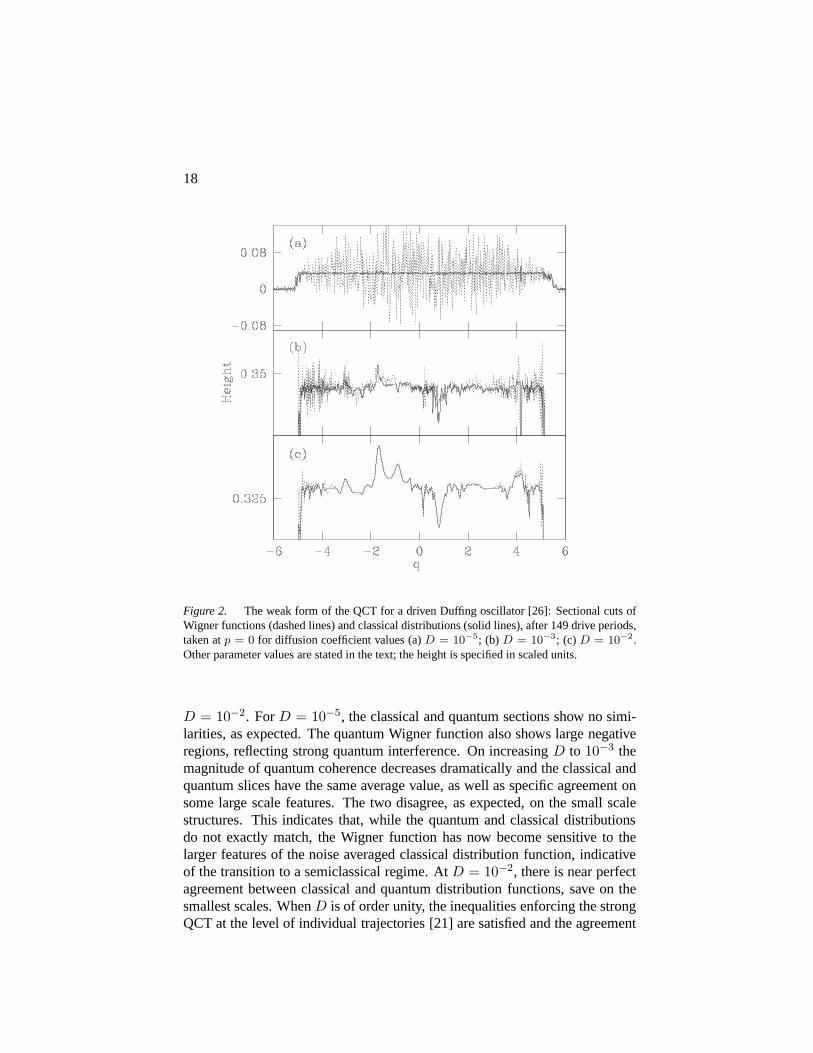
Figure 2. The weak form of the QCT for a driven Duffing oscillator [26]: Sectional cuts ofWigner functions (dashed lines) and classical distributions (solid lines), after 149 drive periods,taken atp = 0 for diffusion coefficient values (a)D = 10−5; (b) D = 10−3; (c) D = 10−2.Other parameter values are stated in the text; the height is specified in scaled units.

D = 10−2. ForD = 10−5, the classical and quantum sections show no simi-larities, as expected. The quantum Wigner function also shows large negativeregions, reflecting strong quantum interference. On increasing D to 10−3 themagnitude of quantum coherence decreases dramatically andthe classical andquantum slices have the same average value, as well as specific agreement onsome large scale features. The two disagree, as expected, onthe small scalestructures. This indicates that, while the quantum and classical distributionsdo not exactly match, the Wigner function has now become sensitive to thelarger features of the noise averaged classical distribution function, indicativeof the transition to a semiclassical regime. AtD = 10−2, there is near perfectagreement between classical and quantum distribution functions, save on thesmallest scales. WhenD is of order unity, the inequalities enforcing the strongQCT at the level of individual trajectories [21] are satisfied and the agreement

Chaos and Quantum Mechanics 19

is essentially exact. However, as indicated by Fig. 2(c), detailed agreement forquantum and classical distribution functions can begin at much smaller valuesof the diffusion constant.

Figure 3. Phase space rendering of the Wigner function at timet = 149 periods of driv-ing [26]. The early time part of the unstable manifold associated with the noise-free dynamicsis shown in blue. The value ofD = 10−3 is not sufficient to wipe out all the quantum interfer-ence which, as expected, is most prominent near turns in the manifold.

For more detailed evidence that, atD = 10−3, one is entering a semiclas-sical regime, in Fig. 3 we superimpose an image of the large scale featuresof the classical unstable manifold on top of the full quantumWigner distri-bution atD = 10−3 after 149 drive periods [case (b) of Fig. 2]. The quan-tum phase space clearly exhibits local interference fringes around the largelobe-like structures associated with the short-time evolution of the unstablemanifold. The appearance of local fringing about classicalstructures is di-rect evidence of a semiclassical evolution, where interference effects appearlocally around the backbone of a classical evolution. This is in sharp contrastto the global diffraction pattern seen forD = 0, where the contributions fromindividual curves cannot be distinguished, suppressing the appearance of anyclassical structure [25].

20

6. Chaos in Quantum Mechanics

At this point, our analysis of measured quantum dynamical systems maybe said to have harmonized quantum and classical mechanics in the sense thatthe strong and weak forms of the QCT have appeared naturally.While this iscertainly pleasing, we wish to go further and ask whether theformalism canbe tested by making predictions that are experimentally verifiable and dependuniquely on the nonlinear nature of the conditioned evolution. One very inter-esting idea is the real-time control of quantum systems using state-estimationas pioneered by Belavkin [35] or direct feedback of the measured classical cur-rent [36]. Although quantum feedback control applications[37] have their ownimportance, we now return to the original burning question:Is there chaos inquantum mechanics?

In a limiting case, the answer is clearly in the affirmative. We have alreadyshown that quantum distributions, provided certain conditions are met, canevolve while staying localized and be only very weakly perturbed by noise. Inthe classical limiting case, we recover localized classical trajectories, and thesecan certainly be chaotic. But what if these conditions are not satisfied?

This is the question addressed and answered in Ref. [38]. By defining andcomputing the Lyapunov exponent for an observed quantum system deep inthe quantum regime, we were able to show that the system dynamics is chaotic.Further, the Lyapunov exponent is not the same as that of the classical dynam-ics that emerges in the classical limit. Since the quantum system in the absenceof measurement is not chaotic, this chaos must emerge as the strength of themeasurement is increased, and we examined the nature of thisemergence.

To do this, we must first make certain that we can quantify the existence ofchaos in a robust way. The rigorous quantifier of chaos in a dynamical systemis the maximal Lyapunov exponent [39]. The exponent yields the (asymptotic)rate of exponential divergence of two trajectories which start from neighbor-ing points in phase space, in the limit in which they evolve toinfinity, andthe neighboring points stay infinitesimally close. The maximal Lyapunov ex-ponent characterizes the sensitivity of the system evolution to changes in theinitial condition: if the exponent is positive, then the system is exponentiallysensitive to initial conditions, and is said to be chaotic. We now discuss howthis notion can be applied to observation-conditioned evolution of quantumexpectation values.

A single quantum mechanical particle is in principle an infinite dimensionalsystem. However, for the purpose of defining an observationally relevant Lya-punov exponent, it is sufficient to use a single projected data stream: let usconsider the expectation value of the position,〈x(t)〉. The important quantityis thus the divergence,∆(t) = |〈x(t)〉 − 〈xfid(t)〉|, between a fiducial trajec-tory and a second trajectory infinitesimally close to it. It is important to keep

Chaos and Quantum Mechanics 21

in mind that the system is driven by noise. Since we wish to examine the sen-sitivity of the system to changes in the initial conditions,and not to changesin the noise, we must hold the noise realization fixed when calculating thedivergence. The Lyapunov exponent is thus

λ ≡ limt→∞

lim∆s(0)→0

ln ∆s(t)

t≡ lim

t→∞λs(t) (25)

where the subscripts denotes the noise realization. This definition is the obvi-ous generalization of the conventional ODE definition to dynamical averages,where the noise is treated as a drive on the system. Indeed, under the conditionswhen (noisy) classical motion emerges, and thus when localization holds, it re-duces to the conventional definition, and yields the correctclassical Lyapunovexponent. To combat slow convergence, we measure the Lyapunov exponentby averaging over an ensemble of finite-time exponentsλs(t) instead of takingthe asymptotic long-time limit for a single trajectory.

A key result now follows: In unobserved, i.e., isolated quantum dynami-cal systems, it is possible to prove, by employing unitarityand the Schwarzinequality, thatλ vanishes; the finite-time exponent,λ(t), decays away as1/t [40]. From the Kosloff-Rice theorem we know, of course, thatthe Lya-punov exponent must be zero, since the overall evolution is integrable, but thisresult gives us a quantitative statement regarding the decay of the exponent. Itturns out that this particular result applies also to the evolution of averages inisolated classical systems and, in this sense, is more general than Kosloff-Rice.As we have emphasized earlier, once measurement is included, the evolutionbecomes nonlinear and the Lyapunov exponent need not vanishclassically orquantum mechanically.

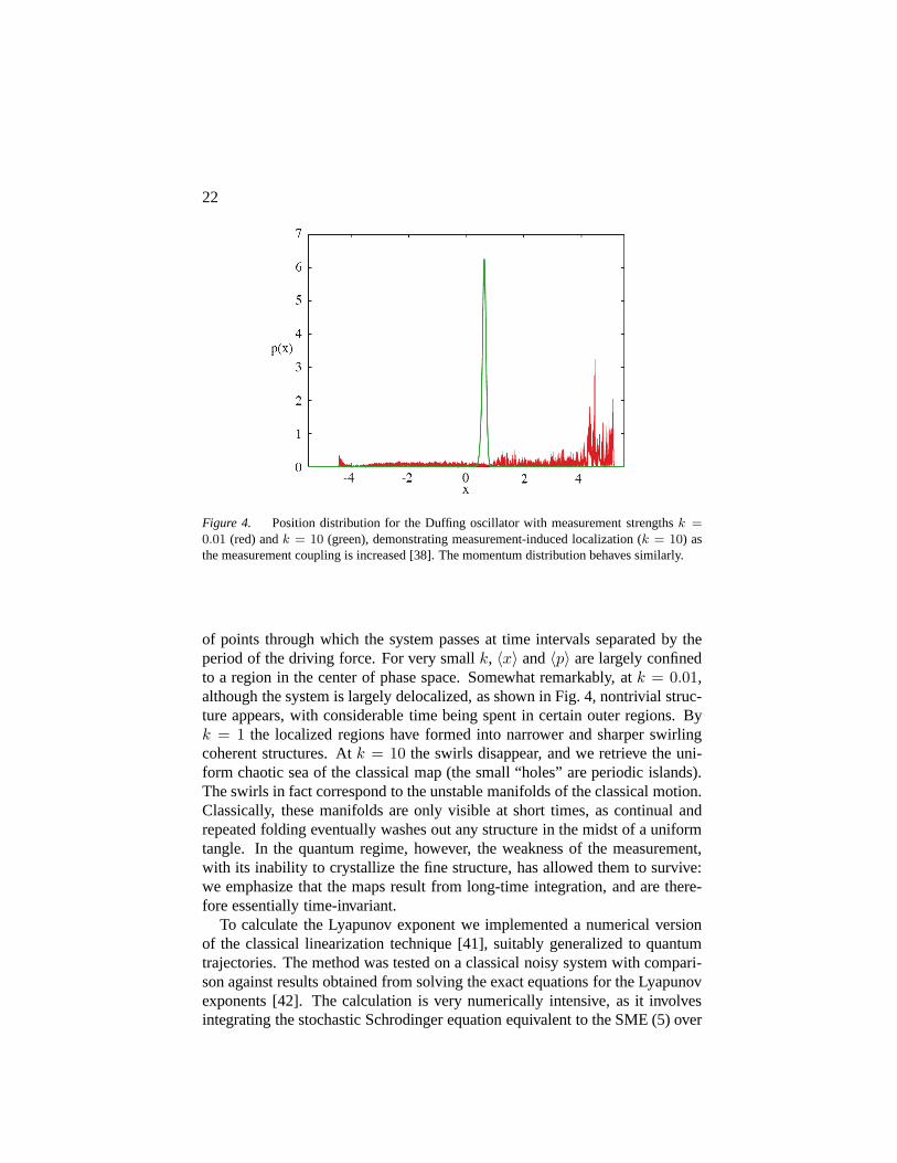
As a particular system of interest, we turn once again to the Duffing os-cillator, this time with h̄ = 10−2, which is small enough so that the sys-tem makes a transition to classical dynamics when the measurement is suf-ficiently strong. As we increase the measurement strength, we can examinethe transformation from essentially isolated quantum evolution all the way tothe known chaos of the classical Duffing oscillator. To examine the emer-gence of chaos, in Ref. [38] we solved for the evolution of thesystem fork = 5×10−4, 10−3, 0.01, 0.1, 1, 10. Whenk ≤ 0.01, the distribution is spreadover the entire accessible region, and Ehrenfest’s theoremis not satisfied. Con-versely, fork = 10, the distribution is well-localized (Fig. 4), and Ehrenfest’stheorem holds throughout the evolution. Since the backaction noise, character-ized by the momentum diffusion coefficient,D = h̄2k, remains small, at thisvalue ofk the motion is that of the classical system, to a very good approxima-tion.

Stroboscopic maps help reveal the global structural transformation in phasespace in going from quantum to classical dynamics (Fig. 5). The maps consist

22

Figure 4. Position distribution for the Duffing oscillator with measurement strengthsk =0.01 (red) andk = 10 (green), demonstrating measurement-induced localization (k = 10) asthe measurement coupling is increased [38]. The momentum distribution behaves similarly.

of points through which the system passes at time intervals separated by theperiod of the driving force. For very smallk, 〈x〉 and〈p〉 are largely confinedto a region in the center of phase space. Somewhat remarkably, at k = 0.01,although the system is largely delocalized, as shown in Fig.4, nontrivial struc-ture appears, with considerable time being spent in certainouter regions. Byk = 1 the localized regions have formed into narrower and sharperswirlingcoherent structures. Atk = 10 the swirls disappear, and we retrieve the uni-form chaotic sea of the classical map (the small “holes” are periodic islands).The swirls in fact correspond to the unstable manifolds of the classical motion.Classically, these manifolds are only visible at short times, as continual andrepeated folding eventually washes out any structure in themidst of a uniformtangle. In the quantum regime, however, the weakness of the measurement,with its inability to crystallize the fine structure, has allowed them to survive:we emphasize that the maps result from long-time integration, and are there-fore essentially time-invariant.

To calculate the Lyapunov exponent we implemented a numerical versionof the classical linearization technique [41], suitably generalized to quantumtrajectories. The method was tested on a classical noisy system with compari-son against results obtained from solving the exact equations for the Lyapunovexponents [42]. The calculation is very numerically intensive, as it involvesintegrating the stochastic Schrodinger equation equivalent to the SME (5) over

Chaos and Quantum Mechanics 23

Figure 5. Phase space stroboscopic maps [38] for the observed Duffing oscillator for 4different measurement strengths,k = 5 × 10−4, 0.01 (top), and 1, 10 (bottom). Contourlines are superimposed to provide a measure of local point density at relative density levels of0.05, 0.15, 0.25, 0.35, 0.45, and0.55.

thousands of driving periods, and averaging over many noiserealizations; par-allel supercomputers were invaluable for this task.

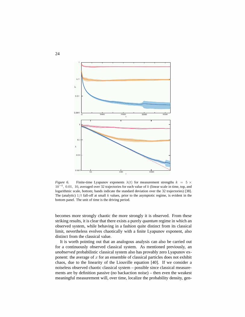
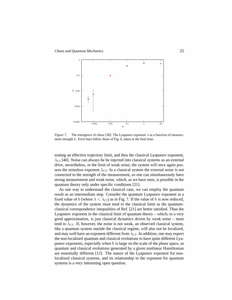
The computations show that ast is increased, for nonzerok, the value ob-tained forλ(t) falls as1/t, following the behavior expected fork = 0, until apoint at which an asymptotic regime takes over, stabilizingat a finite value ofthe Lyapunov exponent ast → ∞. This behavior is shown in Fig. 6 for threevalues ofk. The Lyapunov exponent as a function ofk is shown in Fig. 7. Theexponent increases over two orders of magnitude in an approximately power-law fashion ask is varied from5 × 10−4 to 10, before settling to the classicalvalue,λCl = 0.57. The results in Figs. 6 and 7 show clearly that chaos emergesin the observed quantum dynamics well before the limit of classical motion isobtained.

We also computed the Lyapunov exponent for the quantum system whenits action is sufficiently small that smooth classical dynamics cannot emerge,even for strong measurement [38]. Taking a value ofh̄ = 16, we find that fork = 5 × 10−3, λ = 0.029 ± 0.008, for k = 0.01, λ = 0.046 ± 0.01 andfor k = 0.02, λ = 0.077 ± 0.01. Thus the system is once again chaotic, and

24

Figure 6. Finite-time Lyapunov exponentsλ(t) for measurement strengthsk = 5 ×10−4, 0.01, 10, averaged over 32 trajectories for each value ofk (linear scale in time, top, andlogarithmic scale, bottom; bands indicate the standard deviation over the 32 trajectories) [38].The (analytic)1/t fall-off at small k values, prior to the asymptotic regime, is evident in thebottom panel. The unit of time is the driving period.

becomes more strongly chaotic the more strongly it is observed. From thesestriking results, it is clear that there exists a purelyquantumregime in which anobserved system, while behaving in a fashion quite distinctfrom its classicallimit, nevertheless evolves chaotically with a finite Lyapunov exponent, alsodistinct from the classical value.

It is worth pointing out that an analogous analysis can also be carried outfor a continuously observed classical system. As mentionedpreviously, anunobservedprobabilistic classical system also has provably zero Lyapunov ex-ponent: the average ofx for an ensemble of classical particles does not exhibitchaos, due to the linearity of the Liouville equation [40]. If we consider anoiseless observed chaotic classical system – possible since classical measure-ments are by definition passive (no backaction noise) – then even the weakestmeaningful measurement will, over time, localize the probability density, gen-

Chaos and Quantum Mechanics 25

0.0001

0.001

0.01

0.1

1

0.001 0.01 0.1 1 10k

λ

Figure 7. The emergence of chaos [38]: The Lyapunov exponentλ as a function of measure-ment strengthk. Error-bars follow those of Fig. 6, taken at the final time.

erating an effective trajectory limit, and thus the classical Lyapunov exponent,λCl [40]. Noise can always be be injected into classical systemsas an externaldrive, nevertheless, in the limit of weak noise, the system will once again pos-sess the noiseless exponentλCl: In a classical system the external noise is notconnected to the strength of the measurement, so one can simultaneously havestrong measurement and weak noise, which, as we have seen, ispossible in thequantum theory only under specific conditions [21].

As one way to understand the classical case, we can employ thequantumresult as an intermediate step. Consider the quantum Lyapunov exponent at afixed value ofk (whereλ < λCl) as in Fig. 7. If the value of̄h is now reduced,the dynamics of the system must tend to the classical limit asthe quantum-classical correspondence inequalities of Ref. [21] are better satisfied. Thus theLyapunov exponent in the classical limit of quantum theory –which, to a verygood approximation, is just classical dynamics driven by weak noise – musttend toλCl. If, however, the noise is not weak, an observed classical system,like a quantum system outside the classical regime, will also not be localized,and may well have an exponent different fromλCl. In addition, one may expectthe non-localized quantum and classical evolutions to havequite different Lya-punov exponents, especially whenh̄ is large on the scale of the phase space, asquantum and classical evolutions generated by a given nonlinear Hamiltonianare essentially different [12]. The nature of the Lyapunov exponent for non-localized classical systems, and its relationship to the exponent for quantumsystems is a very interesting open question.

26

7. Concluding Remarks

To summarize, we have presented a simple analysis of continuously ob-served classical and quantum dynamical systems. This analysis is in fact re-quired to deal with next-generation experiments and underlies the nascent fieldof real-time quantum feedback control. Major results include an intuitive andquantitative understanding of the quantum-classical transition. It is pleasingthat both the strong and weak forms of the QCT can eventually be understoodas a macroscopic limit of observed-system quantum mechanics, i.e., wheneverthe observed system actionS ≫ h̄.

Perhaps, most interestingly, we have obtained clear predictions for dynami-cal chaos in observed quantum systems that are far from the classical regime.We emphasize that the chaos identified here is not merely a formal result –even deep in the quantum regime, the Lyapunov exponent can beobtained frommeasurements on a real system as in near-future cavity QED and nanomechan-ics experiments [7]. Experimentally, one would use the known measurementrecord to integrate the SME (5); this provides the time evolution of the meanvalue of the position. From this fiducial trajectory, given the knowledge of thesystem Hamiltonian, the Lyapunov exponent can be obtained by following theprocedure described here.

Acknowledgments

SH thanks the organizers of the 16th Florida Workshop in Nonlinear As-tronomy and Physics, dedicated to the memory of Henry Kandrup, for theirkind invitation to lecture at the meeting. Large-scale parallel computing sup-port from Los Alamos National Laboratory’s Institutional Computing Initiativeis gratefully acknowledged. This research is supported by the Department ofEnergy, under contract W-7405-ENG-36.

References

[1] R. Kosloff and S.A. Rice, J. Chem. Phys.74, 1340 (1981); J. Manz, J. Chem. Phys.91,2190 (1989).

[2] P. Bocchieri and A. Loinger, Phys. Rev.107, 337 (1957); T. Hogg and B.A. Huberman,Phys. Rev. Lett.48, 711 (1982).

[3] J.S. Bell, Phys. World,8, 33 (1990).

[4] B.O. Koopman, Proc. Natl. Acad. Sci. USA17, 31 (1931).

[5] A. Peres,Quantum Theory: Concepts and Methods(Kluwer, Boston, 1993).

[6] P.S. Maybeck,Stochastic Models, Estimation and Control(Academic Press, New York,1982); O.L.R. Jacobs,Introduction to Control Theory(Oxford University Press, Oxford,1993).

[7] H. Mabuchi and A.C. Doherty, Science298, 1372 (2002); M.D. LaHaye, O. Buu, B.Camarota, and K.C. Schwab, Science304, 74 (2004).

Chaos and Quantum Mechanics 27

[8] See, e.g., J.S. Bell,Speakable and unspeakable in quantum mechanics(Cambridge Uni-versity Press, New York, 1988).

[9] L.D. Landau and E.M. Lifshitz,Quantum Mechanics: Non-Relativistic Theory(Perga-mon Press, New York, 1965).

[10] L.D. Landau and E.M. Lifshitz,Statistical Physics(Pergamon Press, New York, 1980).

[11] K. Hepp, Helv. Phys. Acta45, 237 (1972); W.H. Zurek, Phys. Rev. D24, 1516 (1981);ibid 26, 1862 (1982); E. Joos and H.D. Zeh, Z. Phys. B59, 223 (1985).

[12] S. Habib, K. Jacobs, H. Mabuchi, R. Ryne, K. Shizume and B. Sundaram, Phys. Rev.Lett. 88, 040402 (2002).

[13] E.P. Wigner, Phys. Rev.40, 749 (1932); V.I. Tatarskii, Usp. Fiz. Nauk139, 587 (1983)[Sov. Phys. Uspekhi26, 311 (1983)]; M. Hillery, R.F. O’Connell, M.O. Scully, andE.P. Wigner, Phys. Rep.106, 121 (1984).

[14] S. Habib, Phys. Rev. D42, 2566 (1990).

[15] L.P. Kadanoff and G. Baym,Quantum Statistical Mechanics(Addison-Wesley, RedwoodCity, 1989); R. Zwanzig,Nonequilibrium Statistical Mechanics(Oxford University Press,New York, 2001); K. Blum,Density Matrix Theory and Applications(Plenum Press, NewYork, 1996).

[16] L. Diosi, Phys. Lett.129A, 419 (1988); V.P. Belavkin and P. Staszewski, Phys. Lett.140A, 359 (1989); Y. Salama and N. Gisin, Phys. Lett.181A, 269 (1993);C.M. Cavesand G.J. Milburn, Phys. Rev. A36, 5543 (1987); H.M. Wiseman and G.J. Milburn, Phys.Rev. A 47, 642(1993); H.J. Carmichael,An Open Systems Approach to Quantum Optics(Springer-Verlag, Berlin, 1993); G.J. Milburn, Quantum Semiclass. Opt.8, 269 (1996);T.A. Brun, Am. J. Phys.70, 719 (2002); P. Warszawski and H.M. Wiseman, J. Opt. B5,1 (2003).

[17] A.C. Doherty, K. Jacobs, and G. Jungman, Phys. Rev. A63, 062306 (2001).

[18] D.T. Gillespie, Am. J. Phys.64, 225 (1996).

[19] See, e.g., D. Mozyrsky and I. Martin, Phys. Rev. Lett.89, 018301 (2002).

[20] T.P. McGarty,Stochastic Systems and State Estimation(Wiley-Interscience, New York,1974).

[21] T. Bhattacharya, S. Habib and K. Jacobs, Phys. Rev. Lett. 85, 4852 (2000); Phys. Rev.A 67, 042103 (2003). See also, S. Ghose, P. Alsing, I. Deutsch, T.Bhattacharya, andS. Habib, Phys. Rev. A69, 052116 (2004).

[22] See, e.g., S. Habib, quant-ph/0406011

[23] B.V. Chirikov, Chaos1, 95 (1991).

[24] W.A. Lin and L.E. Ballentine, Phys. Rev. Lett.65, 2927 (1990).

[25] S. Habib, K. Shizume, and W.H. Zurek, Phys. Rev. Lett.80, 4361 (1998).

[26] B.D. Greenbaum, S. Habib, K. Shizume, and B. Sundaram, Chaos (in press); quant-ph/0401174

[27] G. Lindblad, Comm. Math. Phys.48, 199 (1976); V. Gorini, A. Kossakowski, andE.C.G. Sudarshan, J. Math. Phys.17, 821 (1976).

[28] A.O. Caldeira and A.J. Leggett, Phys. Rev. A31, 1059 (1985).

[29] M.V. Berry, Phil. Trans. Roy. Soc. A287, 237 (1977); E.J. Heller, J. Chem. Phys.67,3339 (1977).

[30] A.R. Kolovsky, Phys. Rev. Lett.76, 340 (1996).

28

[31] V.P. Maslov and M.V. Fedoriuk,Semi-Classical Approximation in Quantum Mechanics(Reidel, Holland, 1981).

[32] M.V. Berry and N.L. Balazs, J. Phys. A12, 625 (1979).

[33] E.J. Heller and S. Tomsovic, Phys. Today7, 38 (1993); Phys. Rev. E47, 282 (1993).

[34] J. Guckenheimer and P. Holmes,Nonlinear Oscillations, Dynamical Systems, and Bifur-cations of Vector Fields(Springer-Verlag, Berlin, 1986).

[35] V.P. Belavkin, Comm. Math. Phys.146, 611 (1992); V.P. Belavkin, Rep. Math. Phys.43,405 (1999); A.C. Doherty and K. Jacobs, Phys. Rev. A60, 2700 (1999); A.C. Doherty,S. Habib, K. Jacobs, H. Mabuchi, and S.-M. Tan, Phys. Rev. A62, 012105 (2000).

[36] H.M. Wiseman and G.J. Milburn, Phys. Rev. Lett.70, 548 (1993).

[37] See, e.g., H.M. Wiseman, S. Mancini, and J. Wang, Phys. Rev. A 66, 013807 (2002);R. Ruskov and A.N. Korotkov, Phys. Rev. B66, 041401(R) (2002); A. Hopkins, K. Ja-cobs, S. Habib, and K. Schwab, Phys. Rev. B68, 235328 (2003); D.A. Steck, K. Jacobs,H. Mabuchi, T. Bhattacharya, and S. Habib, Phys. Rev. Lett.92, 223004 (2004).

[38] S. Habib, K. Jacobs, and K. Shizume, quant-ph/0412159

[39] J.-P. Eckmann and D. Ruelle, Rev. Mod. Phys.57, 617 (1985).

[40] S. Habib, K. Jacobs, and K. Shizume, in preparation.

[41] A. Wolf, J.B. Swift, H.L. Swinney and J.A. Vastano, Physica16D, 285 (1985).

[42] S. Habib and R.D. Ryne, Phys. Rev. Lett.74, 70 (1995).