Quantum dynamical entropies in discrete classical chaos

arX

iv:m

ath-

ph/0

3080

33v2

9 D

ec 2

003

QUANTUM DYNAMICAL ENTROPIES

IN DISCRETE CLASSICAL CHAOS

FABIO BENATTI

Dipartimento di Fisi a Teori a

Università di Trieste

Strada Costiera 11, 34014 Trieste, Italy

and Istituto Nazionale di Fisi a Nu leare, Sezione di Trieste,


fabio.benattits.infn.it

VALERIO CAPPELLINI

Dipartimento di Fisi a Teori a

Università di Trieste


valerio. appellinits.infn.it

FEDERICO ZERTUCHE

Instituto de Matemáti as, UNAM

Unidad Cuernava a, A.P. 273-3, Admon. 3

62251 Cuernava a, Morelos, Méxi o.

zertu hemat uer.unam.mx

17th De ember 2013

Abstra t

We dis uss ertain analogies between quantization and dis retization of las-

si al systems on manifolds. In parti ular, we will apply the quantum dy-

nami al entropy of Ali ki and Fannes to numeri ally study the footprints of

haos in dis retized versions of hyperboli maps on the torus.

Short Title: Quantum Dynami al Entropies in Dis rete Classi al Chaos

Keywords: Chaos, Symboli Dynami s, Kolmogorov Entropy, Algorithmi Infor-

mation

1

http://arxiv.org/abs/math-ph/0308033v2

2 F. Benatti, V. Cappellini and F. Zertu he

Contents

1 Introdu tion. 2

2 Automorphisms on the Torus 4

2.1 Weyl dis retization . . . . . . . . . . . . . . . . . . . . . . . . . . 6

3 Kolmogorov metri entropy 9

3.1 Symboli Models as Classi al Spin Chains . . . . . . . . . . . . . . 10

4 ALFEntropy 11

4.1 ALFEntropy for Dis retized (X , µ, Tα) . . . . . . . . . . . . . . . . 14

5 Analysis of entropy produ tion 18

5.1 The ase of Tα ∈ GL2 (T2) . . . . . . . . . . . . . . . . . . . . . . . 20

5.1.1 Hyperboli regime with D randomly hosen points ri in Λ . 20

5.1.2 Hyperboli regime with D nearest neighbors ri in Λ . . . . . 21

5.1.3 Ellipti regime (α ∈ −1,−2,−3) . . . . . . . . . . . . . . 23

5.1.4 Paraboli regime (α ∈ 0, 4) . . . . . . . . . . . . . . . . . 24

5.2 The ase of Sawtooth Maps . . . . . . . . . . . . . . . . . . . . . . 25

6 Con lusions 28

1. Introdu tion.

Classi al haos is asso iated with motion on a ompa t phasespa e with high

sensitivity to initial onditions: traje tories diverge exponentially fast and never-

theless remain onned to bounded regions [1, 2, 3.

In dis rete times, su h a behaviour is hara terized by a positive Lyapounov

exponent log λ, λ > 1, and by a onsequent spreading of initial errors δ su h

that, after n timesteps, δ 7→ δn ≃ δ λn. Exponential ampli ation on a ompa t

phasespa e annot grow indenitely, therefore the Lyapounov exponent an only

be obtained as:

log λ := limt→∞

1

nlimδ→0

log

(δnδ

),

Quantum Dynami al Entropies in Dis rete Classi al Chaos 3

that is by rst letting δ → 0 and only afterwards n→ ∞.

In quantum me hani s non ommutativity entails absen e of ontinuous tra-

je tories or, semi lassi ally, an intrinsi oarse-graining of phasespa e determined

by Plan k's onstant ~: this forbids δ (the minimal error possible) to go to zero.

Thus, if haoti behaviour is identied with log λ > 0, then it is quantally sup-

pressed, unless, performing the lassi al limit rst, we let room for δ → 0 [4.

In dis rete lassi al systems, one deals with dis retized versions of ontinuous

lassi al systems or with ellular automata [5, 6, 7 with nite number of states.

In this ase, roughly speaking, the minimal distan e between two states or on-

gurations is stri tly larger than zero; therefore, the reason way log λ is trivially

zero is very mu h similar to the one en ountered in the eld of quantum haos,

its origin being now not in non ommutativity but in the la k of a ontinuous

stru ture. Alternative methods have thus to be developed in order to deal with

the granularity of phasespa e [8, 9, 5, 6, 7.

An entropi approa h is likely to oer a promising perspe tive. For su-

iently smooth lassi al ontinuous systems, the exponential spreading of errors is

equivalent to a net entropy produ tion, better known as Kolmogorov dynami al,

or metri , entropy [3. The phasespa e is partitioned into ells by means of whi h

any traje tory is en oded into a sequen e of symbols. As times goes on, the ri h-

ness in dierent symboli traje tories ree ts the irregularity of the motion and is

asso iated with stri tly positive dynami al entropy [10.

A frequen y approa h to the numeri al evaluation of the entropy produ tion

has re ently been applied in dis retized version of various haoti ontinuous las-

si al dynami al systems [11. In this paper, we suggest a dierent strategy: mo-

tivated by the similarities between quantization and dis retization of ontinuous

lassi al dynami al systems, we propose to use the quantum dynami al entropy

re ently introdu ed by Ali ki and Fannes [12,13, whi h we shall refer to as ALF

entropy.

The ALFentropy is based on the algebrai properties of dynami al systems,

that is on the fa t that, independently on whether they are ommutative or not,

they are des ribable by suitable algebras of observables, their time evolution by

linear maps on these algebras and their states by expe tations over them.

As su h, the ALFentropy applies equally well to lassi al and quantum sys-

tems, and redu es to the Kolmogorov entropy in the former ase. In parti ular, it

has been showed that it allows a quite straightforward al ulation of the Lyapounov

exponents of Arnold at maps on Ddimensional tori [14.

In this paper we aim at showing how the ALFentropy may be of use in a

dis rete lassi al ontext, pre isely when 2dimensional at maps are for ed to live

on a square latti e with spa ing

1N

(N integer), with parti ular fo us upon the


emergen e of the ontinuous behaviour when N 7−→ ∞.

In quantum me hani s, the lassi al limit is a hieved when ~ → 0. Analo-

gously, in the ase of dis rete lassi al systems, by letting the minimal distan e

between states go to zero, one might hope to re over a well dened ontinuous

dynami al system, perhaps a haoti one. Also, very mu h as in the semi lassi al

approximation, one expe ts the possibility of mimi king the behaviour of dis rete

systems by means of that of their ontinuous limits and vi e versa. However, this

is possible only up to a time τB, alled breakingtime [4; it an be heuristi ally

estimated as the time when the minimal error permitted, δ, be omes of the order

of the phasespa e bound ∆. Therefore, when, in the ontinuum, a Lyapounov

exponent log λ > 0 is present, the breakingtime s ales as τB =1

log λlog

∆

δ.

In the following, we shall onsider dis rete dynami al systems obtained by

dis retizing a sub lass of the Unitary Modular Group of (2dimensional) Toral

Automorphisms [3 ontaining the well known Arnold Cat Maps. We shall provide:

• the algebrai setting for the ontinuous limit N 7−→ ∞;

• the te hni al framework to onstru t the ALFentropy and numeri al short-

uts to ompute it;

and study:

• the behaviour of the entropy produ tion and how the breakingtime τB is

rea hed in hyperboli systems;

• the dieren es in behavior between hyperboli and ellipti systems;

• the distribution of eigenvalues of the multitime orrelation matrix used in

omputing the ALFentropy;

• the behaviour of the entropy produ tion in the ase of Sawtooth Maps [15,

16, 17 whi h are dis ontinuous on the 2dimensional torus.

2. Automorphisms on the Torus

Usually, ontinuous lassi al motion is des ribed by means of a measure spa e X ,

the phasespa e, endowed with the Borel σalgebra and a normalized measure µ,

µ(X ) = 1. The volumes µ(E) =

∫

E

dµ(x) of measurable subsets E ⊆ X represent

the probabilities that a phasepoint x ∈ X belong to them. By spe ifying the

statisti al properties of the system, the measure µ denes a state of it.


In su h a s heme, a reversible dis rete time dynami s amounts to an invertible

measurable map T : X 7→ X su h that µT = µ and to its iterates T jj∈Z. Phasetraje tories passing through x ∈ X at time 0 are then sequen es T jxj∈Z [3.

Classi al dynami al systems are thus onveniently des ribed by triplets (X , µ, T );in the following, we shall on entrate on triplets (X , µ, Tα), where

X = T

2 = R

2/Z2 = x = (x1, x2) (mod 1) (1a)

Tα

(x1

x2

)=

(1 + α 1α 1

) (x1

x2

)(mod 1) , α ∈ Z (1b)

dµ(x) = dx1 dx2 · (1 )

Remarks 2.1

i. Sin e det (Tα) = 1, the Lebesgue measure dened in (1 ) is invariant

for all α ∈ Z;ii. The eigenvalues of ( 1+α 1

α 1 ) are (α+ 2±√

(α+ 2)2 − 4)/2. They are

onjugate omplex numbers if α ∈ [−4, 0], while one eigenvalue λ is

greater than 1 if α 6∈ [−4, 0]. In this ase, distan es are stret hed

along the dire tion of the eigenve tor |e+〉, Sα|e+〉 = λ|e+〉, on-tra ted along that of |e−〉, Sα|e−〉 = λ−1|e−〉.For su h α's all periodi points are hyperboli [17.

iii. T1 = ( 2 11 1 ) is the Arnold Cat Map [3. Then, T1 ∈ Tαα∈Z ⊂

SL2

(T

2)⊂ GL2

(T

2)⊂ ML2

(T

2)where ML2 (T2) is the subset of

2× 2 matri es with integer entries, GL2 (T2) the subset of invertiblematri es and SL2 (T2) the subset of matri es with determinant one.

iv. The dynami s generated by Tα ∈ SL2 (T2) is alled Unitary Modular

Group [3 (UMG for short).

For future omparison with quantum dynami al systems, we adopt an algebrai

point of view and argue in terms of lassi al observables, pre isely in terms of

omplex ontinuous fun tions f on X = T

2.

• These fun tions form a C* algebra AX = C0 (X ) with respe t to the topology

given by the uniform norm ‖f‖0 = supx∈X

∣∣∣f (x)∣∣∣;

• the Lebesgue measure µ denes a state ωµ on AX whi h evaluates mean

values of observables via integration:

f 7→ ωµ(f) :=

∫

X

dx f(x) ; (2)


• the dis retetime dynami s Tα : X 7→ X generates the dis rete group of

automorphisms Θjα : AX 7→ AX , given by

Θjα (f) (x) = f(Sjα (x)) , j ∈ Z , (3)

that preserve the state, ωµ Θjα = ωµ.

Denition 2.1

The dynami al systems (X , µ, Tα) will be identied by the algebrai

triplets (AX , ωµ,Θα).

2.1. Weyl dis retization

In the following we shall pro eed to a dis retization of the systems introdu ed in

the previous Se tion and to the study of how haos emerges when the ontinuous

limit is being rea hed.

Roughly speaking, given an integer N , we shall for e the ontinuous lassi al

systems (AX , ωµ,Θα) to live on a latti e LN ⊂ T

2given by:

LN := p

N

∣∣∣ p ∈ (Z/NZ)2, (4)

where (Z/NZ) denotes the residual lass (mod N).

A good indi ator of haos in ontinuous dynami al systems is the metri en-

tropy of Kolmogorov [3 (see Se tion 3 below). We an ompare dis retization of

lassi al ontinuous systems with quantization; in this way, we an protably use a

quantum extension of the metri entropy whi h will be presented in Se tion 4. To

this aim, we dene a dis retization pro edure resembling Weyl quantization [18,19;

in pra ti e, we will onstru t a *morphism JN,∞ fromAX = C0 (X ) into the abelianalgebra DN2 (C) of N2 ×N2

matri es whi h are diagonal with respe t to a hosen

orthonormal basis |ℓ〉ℓ∈(Z/NZ)2. The basis ve tors will be labeled by the points

of a square grid of latti e spa ing

1N

with 0 6 ℓi 6 (N − 1) (N identied with 0)superimposed onto X = T

2.

In order to dene JN,∞, we use Fourier analysis and restri t ourselves to the

*subalgebra Wexp

∈ AX generated by the exponential fun tions

W (n)(x) = exp(2πi n · x) , (5)

where n = (n1, n2) ∈ Z2and n · x = n1 x1 + n2 x2. The generi element of W

exp

is:

f(x) =∑

n∈Z2

fnW (n)(x) (6)


with nitely many oe ients fn =

∫∫

X

dx f(x) e−2πinxdierent from zero.

On Wexp

, formula (2) denes a state su h that

ωµ (W (n)) = δn,0· (7)

Further, sin e n · (Tα x) = (T trα n) · x, the automorphisms (3) map exponentials

into themselves:

Θα (W (n)) = W (T tr

α · n) , T tr

α =

(1 + α α

1 1

)(8)

Remark 2.2

The latter property no longer holds when α 6∈ Z as will be the ase in

Se tion 5.2 where we deal with Sawtooth Maps [15, 16, 17.

Following Weyl quantization, we get elements of DN2out of elements of W

exp

by

repla ing, in (6), exponentials with diagonal matri es:

W (n) 7−→ W (n) :=∑

ℓ∈(Z/NZ)2

e2πinℓ

N |ℓ〉〈ℓ | , ℓ = (ℓ1, ℓ2) · (9)

Denition 2.2

We will denote by JWN,∞, the *morphism from the *algebra W

exp

into

the diagonal matrix algebra DN2 (C), given by:

Wexp

∋ f 7−→ JWN,∞(f) :=

∑

n∈Z2

fn W (n)

=∑

ℓ∈(Z/NZ)2

f

(ℓ

N

)|ℓ〉〈ℓ | · (10)

Remarks 2.3

i) The ompletion of the subalgebra W∞ with respe t to the uniform

norm ‖f‖0 = supx∈X

∣∣∣f (x)∣∣∣ is the C* algebra AX = C0 (X ) [20.

ii) The *morphismJWN,∞ : W

exp

7→ DN2 (C) is bounded bywwJW

N,∞

ww = 1.

Using the Bounded Limit Theorem [20, JWN,∞ an be uniquely ex-

tended to a bounded linear transformation (with the same bound)

JN,∞ : AX 7−→ DN2 (C).

iii) JN,∞ (AX ) = DN2 (C).


We go ba k from DN2 (C) to a *algebra of fun tions on X by dening a *morphism

J∞,N that inverts JN,∞ in the N → ∞ limit. In the Weyl quantization the in-

verting *morphism is onstru ted by means of oherent states |β (x)〉, x ∈ X ,

with good lo alization properties in X .

Denition 2.3

We will denote by J∞,N : DN2 (C) 7−→ AX the *morphism dened by:

DN2 (C) ∋M 7−→ J∞,N(M) (x) := 〈β (x) |M |β (x)〉 , (11)

where |β (x)〉 are oherent ve tors in HN2 = C

N2

We now onstru t a suitable family of |β (x)〉: we shall denote by ⌊·⌋ and 〈·〉 theinteger and fra tional part of a real number so that we an express ea h T

2as

x =(

⌊Nx1⌋N

, ⌊Nx2⌋N

)+

(〈Nx1〉N

, 〈Nx2〉N

). Then we asso iate x ∈ T

2with ve tors of

HN2as follows:

x 7→ |β (x)〉 = λ11 (x) |⌊Nx1⌋ , ⌊Nx2⌋〉+

+ λ12 (x) |⌊Nx1⌋ , ⌊Nx2⌋ + 1〉 + λ21 (x) |⌊Nx1⌋ + 1, ⌊Nx2⌋〉+

+ λ22 (x) |⌊Nx1⌋ + 1, ⌊Nx2⌋ + 1〉 · (12)

We hoose the oe ients λij so that ‖β (x)‖ = 1 and that the map (12) be

invertible:

λ11 (x) = cos(π2〈Nx1〉

)cos

(π2〈Nx2〉

)

λ12 (x) = cos(π2〈Nx1〉

)sin

(π2〈Nx2〉

)

λ21 (x) = sin(π2〈Nx1〉

)cos

(π2〈Nx2〉

)

λ22 (x) = sin(π2〈Nx1〉

)sin

(π2〈Nx2〉

)(13)

Therefore, from denitions 2.2 and 2.3 it follows that, when mapping AX onto

DN2 (C) and the latter ba k into AX , we get:

fN (x) := (J∞,N JN,∞) (f) (x) =∑

ℓ∈(Z/NZ)2

f

(ℓ

N

) ∣∣⟨β (x)∣∣ℓ

⟩∣∣2 =

=1

4

∑

(µ,ν,ρ,σ)∈0,14

cos (πµ 〈Nx1〉) cos (πν 〈Nx2〉) (−1)µρ+νσ×

× f

(⌊Nx1⌋ + ρ

N,⌊Nx2⌋ + σ

N

)(14)

Remarks 2.4


i) From (14), f = fN on the latti e points. Moreover, although the rst

derivative of (14) is not dened on the latter, its limit exists there

and it is zero; thus, we an extend by ontinuity fN to a fun tion in

C1 (T2) that we will denote again as fN .

ii) We note that Ran (J∞,N) is a subalgebra stri tly ontained in AX ;

this is not surprising and omes as onsequen e of Weyl quantization,

where this phenomenon is quite typi al [18, 19.

We show below that J∞,N JN,∞ approa hes 1AX(the identity fun tion in AX )

when N → ∞. Indeed, a request upon any sensible quantization pro edure is to

re over the lassi al des ription in the limit ~ → 0; in a similar way, our dis retiza-

tion should re over the ontinuous system in the

1N

→ 0 limit.

Theorem 1 Given f ∈ AX = C0 (T2) , limN→∞

∥∥∥∥ (J∞,N JN,∞ − 1AX) (f)

∥∥∥∥ = 0 ·

Proof: Sin e X = T

2is ompa t, f is uniformly ontinuous on it. Further,

denoting x =⌊Nx⌋N

+〈Nx〉N

, 0 6 〈Nx〉 < 1 implies

wwwwx − ⌊Nx⌋N

wwww −−→N

0;

therefore, for all ε > 0 there exists Nf,ε su h that

N > Nf,ε =⇒∣∣∣∣f (x) − f

(⌊Nx⌋N

) ∣∣∣∣ <ε

2,

uniformly in x. Moreover, a ording to Remark 2.4 (i.), fN ∈ C0 (T2), thus the

previous inequality holds for fN , too. Sin e fN = f on

⌊Nx⌋N

, it follows that, for

su iently large N ,

∣∣∣f (x) − fN (x)∣∣∣ 6

∣∣∣∣f (x) − f

(⌊Nx⌋N

)∣∣∣∣ +

∣∣∣∣ fN(⌊Nx⌋

N

)− fN (x)

∣∣∣∣ 6 ε ,

uniformly in x.

3. Kolmogorov metri entropy

For ontinuous lassi al systems (X , µ, Tα) su h as those introdu ed in Se tion 2,

the onstru tion of the dynami al entropy of Kolmogorov is based on subdividing

X into measurable disjoint subsets Eℓℓ=1,2,··· ,D su h that

⋃ℓEℓ = X whi h form

nite partitions ( oarse grainings) E .Under the dynami al maps Tα in (1b), any given E evolves into T−j

α (E) withatoms T−j

α (Eℓ) = x ∈ X : T jαx ∈ Eℓ; one an then form ner partitions E[0,n−1]


whose atoms Ei0 i1···in−1:= Ei0

⋂T−1α (Ei1) · · ·

⋂T−n+1α (Ein−1) have volumes

µi0 i1···in−1:= µ

(Ei0 ∩ T−1

α (Ei1) · · · ∩ T−n+1α (Ein−1)

). (15)

Denition 3.1

We shall set i = i0 i1 · · · in−1 and denote by ΩnD the set ofDn

n_tuples

with ij taking values in 1, 2, · · · , D.

The atoms of the partitions E[0,n−1] des ribe segments of traje tories up to time

n en oded by the atoms of E that are traversed at su essive times. The ri hness

in diverse traje tories, that is the degree of irregularity of the motion (as seen

with the a ura y of the given oarse-graining), an be measured by the Shannon

entropy [10

Sµ(E[0,n−1]) := −∑

i∈ΩnD

µi logµi . (16)

On the long run, E attributes to the dynami s an entropy per unit timestep

hµ(Tα, E) := limn→∞

1

nSµ(E[0,n−1]) . (17)

This limit is well dened [3 and the Kolmogorov entropy hµ(Tα) of (AX , ωµ,Θα)is dened as the supremum over all nite measurable partitions [3, 10:

hµ(Tα) := supEhµ(Tα, E) · (18)

3.1. Symboli Models as Classi al Spin Chains

Finite partitions E ofX provide symboli models for the dynami al systems (X , µ, Tα)of Se tion 2, whereby the traje tories T jαxj∈Z are en oded into sequen es ijj∈Zof indi es relative to the atoms Eij visited at su essive times j; the dynami s or-

responds to the rightshift along the symboli sequen es. The en oding an be

modelled as the shift along a lassi al spin hain endowed with a shiftinvariant

state [12. This will help to understand the quantum dynami al entropy whi h will

be introdu ed in the next Se tion.

Let D be the number of atoms of a partition E of X , we shall denote by AD

the diagonal D×D matrix algebra generated by the hara teristi fun tions eEℓof

the atoms Eℓ and by A[0,n−1]D the n-fold tensor produ t of n opies of (AD), that

is the Dn ×Dndiagonal matrix algebra A

[0,n−1]D := (AD)0 ⊗ (AD)1 · · · ⊗ (AD)n−1.

Its typi al elements are of the form a0 ⊗ a1 · · · ⊗ an−1 ea h aj being a diagonal


D×D matrix. Every A[p,q]D := ⊗q

j=p(AD)j an be embedded into the innite tensor

produ t A∞D := ⊗∞

k=0(AD)k as

(1)0 ⊗ · · · ⊗ (1)p−1 ⊗ (AD)p ⊗ · · · ⊗ (AD)q ⊗ (1)q+1 ⊗ (1)q+2 ⊗ · · · (19)

The algebra A∞D is a lassi al spin hain with a lassi al Dspin at ea h site.

By means of the dis rete probability measure µii∈ΩnD, one an dene a om-

patible family of states on the lo al algebras A[0,n−1]D :

ρ[0,n−1]E (a0 ⊗ · · · ⊗ an−1) =

∑

i∈ΩnD

µi (a0)i0i0 · · · (an−1)in−1in−1 . (20)

Indeed, let ρN denote the restri tion to a subalgebra N ⊆ M of a state ρ on

a larger algebra M . Sin e

∑in−1

µi0i1···in−1 = µi0i1···in−2 , when n varies the lo al

states ρ[0,n−1]E are su h that ρ

[0,n−1]E A[0,n−2]

D = ρ[0,n−2]E and dene a global state

ρE on A∞D su h that ρEA

[0,n−1]D = ρ

[0,n−1]E .

From the Tα-invarian e of µ it follows that, under the rightshift σ : A∞D 7→ A∞

D ,

σ(A

[p,q]D

)= A

[p+1,q+1]D , (21)

the state ρE of the lassi al spin hain is translation invariant:

ρE σ (a0 ⊗ · · · ⊗ an−1) = ρE ((1)0 ⊗ (a0)1 ⊗ · · · ⊗ (an−1)n)

= ρE (a0 ⊗ · · · ⊗ an−1) · (22)

Finally, denoting by |j〉 the basis ve tors of the representation where the matri es

a ∈ AD are diagonal, lo al states amount to diagonal density matri es

ρ[0,n−1]E =

∑

i∈ΩnD

µi |i0〉〈i0| ⊗ |i1〉〈i1| ⊗ · · · ⊗ |in−1〉〈in−1| , (23)

and the Shannon entropy (16) to the Von Neumann entropy

Sµ(E[0,n−1]) = −Tr[ρ

[0,n−1]E log ρ

[0,n−1]E

]=: Hµ

[E[0,n−1]

]. (24)

4. ALFEntropy

From an algebrai point of view, the dieren e between a triplet (M, ω,Θ) des rib-ing a quantum dynami al system and a triplet (AX , ωµ,Θα) as in Denition 2.1 is

that ω and Θ are now a Θinvariant state, respe tively an automorphism over a

non ommutative (C* or Von Neumann) algebra of operators.


Remark 4.1

In nite dimension D, M is the full matrix algebra of D×D matri es,

the states ω are given by density matri es ρω, su h that ω(X) := Tr(ρωX),while the reversible dynami s Θ is unitarily implemented: Θ(X) =UXU∗

.

The quantum dynami al entropy proposed in [12 by Ali ki and Fannes, ALF

entropy for short, is based on the idea that, in analogy with what one does for

the metri entropy, one an model symboli ally the evolution of quantum systems

by means of the right shift along a spin hain. In the quantum ase the nite

dimensional matrix algebras at the various sites are not diagonal, but, typi ally,

full matrix algebras, that is the spin at ea h site is a quantum spin.

This is done by means of so alled partitions of unit, that is by nite sets

Y =y1, y2, . . . , yD

of operators in a Θinvariant subalgebra M0 ∈ M su h that

D∑

ℓ=1

y∗ℓyℓ = 1 , (25)

where y∗j denotes the adjoint of yj . With Y and the state ω one onstru ts the

D ×D matrix with entries ω(y∗jyi ); su h a matrix is a density matrix ρ[Y ]:

ρ[Y ]i,j := ω(y∗jyi ) · (26)

It is thus possible to dene the entropy of a partition of unit as ( ompare (24)):

Hω[Y ] := −Tr(ρ[Y ] log ρ[Y ]

)· (27)

Further, given two partitions of unit Y =(y0, y1, . . . , yD

), Z =

(z0, z1, . . . , zB

),

of size D, respe tively B, one gets a ner partition of unit of size BD as the set

Y Z :=(y0z0, · · · , y0zB; y1z0, · · · , y1zB; · · · ; yDz0, · · · , yDzB

)· (28)

After j timesteps, Y evolves into Θj(Y) :=

Θj(y1),Θj(y2), · · · ,Θj(yD)

. Sin e

Θ is an automorphism, Θj (Y) is a partition of unit; then, one renes Θj(Y),0 6 j 6 n− 1, into a larger partition of unit

Y [0,n−1] := Θn−1(Y) Θn−2(Y) · · · Θ(Y) Y· (29)

We shall denote the typi al element of

[Y [0,n−1]

]by

[Y [0,n−1]

]i= Θn−1

(yin−1

)Θn−2

(yin−2

)· · · Θ(yi1) yi0· (30)


Ea h renement is in turn asso iated with a density matrix ρ[0,n−1]Y := ρ

[Y [0,n−1]

]

whi h is a state on the algebra M[0,n−1]D := ⊗n−1

ℓ=0 (MD)ℓ, with entries

[ρ[Y [0,n−1]

]]

i,j

:= ω(y∗j0Θ

(y∗j1

)· · ·Θn−1

(y∗jn−1

yin−1

)· · ·Θ

(yi1

)yi0

)· (31)

Moreover ea h renement has an entropy

Hω

[Y [0,n−1]

]= −Tr

(ρ[Y [0,n−1]

]log ρ

[Y [0,n−1]

])· (32)

The states ρ[0,n−1]Y are ompatible: ρ

[0,n−1]Y M

[0,n−2]D = ρ

[0,n−2]Y , and dene a global

state ρY on the quantum spin hain M∞D := ⊗∞

ℓ=0(MD)ℓ.

Then, as in the previous Se tion, it is possible to asso iate with the quantum

dynami al system (M, ω,Θ) a symboli dynami s whi h amounts to the right

shift, σ : (MD)ℓ 7→ (MD)ℓ+1, along the quantum spin half hain ( ompare (21)).

Non ommutativity makes ρY not shiftinvariant, in general [12. In this ase,

the existen e of a limit as in (17) is not guaranteed and one has to dene the

ALFentropy of (M, ω,Θ) as

hALFω,M0(Θ):= sup

Y⊂M0

hALFω,M0(Θ,Y) , (33a)

where hALFω,M0(Θ,Y) := lim sup

n

1

nHω

[Y [0,n−1]

]· (33b)

Like the metri entropy of a partition E , also the ALFentropy of a partition of

unit Y an be physi ally interpreted as an asymptoti entropy produ tion relative

to a spe i oarsegraining.

Remark 4.2

The ALFentropy redu es to the Kolmogorov metri entropy on las-

si al systems. This is best seen by using an algebrai hara teri-

zation of (X , µ, Tα) by means of the Von Neumann algebra MX =L∞µ (X ) of essentially bounded fun tions on X [20. The hara ter-

isti fun tions of measurable subsets of X onstitute a *subalgebra

M0 ⊆ MX ; moreover, given a partition E of X , the hara teristi fun -

tions eEℓof its atoms Eℓ, ZE = eE1, · · · , eED

is a partition of unit

in M0. From (3) it follows that Θjα(eEℓ

) = eT−jα (Eℓ)

and from (2) that[ρ[Z [0,n−1]

E

]]i,j

= δi,j µi (see (15)), when e Hω

[Z [0,n−1]

E

]= Sµ

(E[0,n−1]

)

(see (16) and (27)). In su h a ase, the lim sup in (33b) is a tually

a true limit and yields (17). In [14, the same result is obtained by

means of the algebra AX and of the *subalgebra Wexp

of exponential

fun tions.


4.1. ALFEntropy for Dis retized (X , µ, Tα)

We now return to the lassi al systems (AX , ωµ,Θα) of Se tion 2. For later use,

we introdu e the following map dened on the torus T

2([0, N)2)

, namely [0, N)2

(mod N), and on its subset (Z/NZ)2:

T

2([0, N)2) ∋ x 7→ Uα (x) := N Tα

( x

N

)∈ T2

([0, N)2)

(34)

The use of the *morphisms JN,∞ and J∞,N introdu ed in Se tion 2.1, makes it

onvenient to dene the dis retized versions of (AX , ωµ,Θα) as follows:

Denition 4.1

A dis retization of (AX , ωµ,Θα) is the triplet(DN2 (C) , ωN2 , Θα

)where:

DN2 (C) is the abelian algebra of diagonal matri es a ting on C

N2.

ωN2is the tra ial state given by the expe tation:

DN2 (C) ∋M 7→ ωN2 (M) :=1

N2Tr (M) . (35)

Θα is the *automorphism of DN2 (C) dened by:

DN2 (C) ∋M 7→ Θα (M) :=∑

ℓ∈(Z/NZ)2

MUα(ℓ),Uα(ℓ) |ℓ〉〈ℓ | · (36)

Remarks 4.3

i. The expe tation ωN2 (JN,∞ (f)) orresponds to the numeri al al u-

lation of the integral of f realized on a N ×N grid on T

2.

ii. Θα is a *automorphism be ause the map (Z/NZ)2 ∋ ℓ 7−→ Uα (ℓ) is

a bije tion. For the same reason the state ωN2is Θαinvariant.

iii. One an he k that, given f ∈ AX ,

Θα (JN,∞ (f)) :=∑

ℓ∈(Z/NZ)2

f

(Uα (ℓ)

N

)|ℓ〉〈ℓ | · (37)

iv. Also, Θjα JN,∞ = JN,∞ Θj

α for all j ∈ Z.v. On the ontrary, for j ∈ N, Θj

α JN,∞ 6= JN,∞ Θjα for the Sawtooth

Maps, that is when α 6∈ Z.


The automorphism Θα an be rewritten in the more familiar form

Θα (X) =∑

ℓ∈(Z/NZ)2

XUα(ℓ),Uα(ℓ) |ℓ〉〈ℓ |

=∑

U−1α (s)∈(Z/NZ)2

Xs,s

∣∣U−1α (s)

⟩ ⟨U−1α s

∣∣

(see Remark 4.4 i and ii) = Uα,N

∑

all equiv.

lasses

Xs,s |s〉〈s |

U∗

α,N (38)

= Uα,N X U∗α,N , (39)

where the operators Uα,N era dened by

HN2 ∋∣∣ℓ

⟩7−→ Uα,N

∣∣ℓ⟩:=

∣∣U−1α (ℓ)

⟩· (40)

Remarks 4.4

i) All of Tα, T−1α , T tα and (T−1

α )tbelong to SL2 (Z/NZ); in parti ular

these matri es are automorphisms on (Z/NZ)2so that, in (38), one

an sum over the equivalen e lasses.

ii) The same argument as before proves that the operators in (40) are

unitary whi h is equivalent to saying that Θα is a *automorphism.

In order to onstru t the ALFentropy, we now seek a useful partition of unit in

(DN2 , ωN2, Θα); we do that by means of the subalgebra W∞ ⊆ AX in equations (5

6):

Y :=

yj

D

j=1

=

1√D

exp (2πirj · x)

D

j=1

, (41)

where

rj

D

j=1

=: Λ ⊂ (Z/NZ)2· (42)

Denition 4.2

Given a subset Λ of the latti e onsisting of the points rj as in (42),

we shall denote by Y the partition of unit in (DN2, ωN2 , Θα) given by:

Y =

yj

D

j=1

:=

JN,∞ (yj)

D

j=1

=

1√DW (rj)

D

j=1

, (43)

with W (rj) dened in (9).


From the above denition, the elements of the rened partitions in (30) take the

form:

[Y [0,n−1]

]i=

1

N

1

Dn2

∑

ℓ∈(Z/NZ)2

e2πiN [rin−1

·Un−1α (ℓ)+ ···+ri1

·Uα(ℓ)+ri0·ℓ] |ℓ〉〈ℓ | · (44)

Then, the multitime orrelation matrix ρ[0,n−1]

Yin (31) has entries:

[ρ[Y [0,n−1]

]]

i,j

=1

N2

1

Dn

∑

ℓ∈(Z/NZ)2

e2πiN

n−1∑p=0

(rip−rjp)·Upα(ℓ)

, U0α (ℓ) = 1 (45)

=∑

ℓ∈(Z/NZ)2

〈i| gℓ (n)〉〈gℓ (n)| j〉 , (46)

with 〈i| gℓ (n)〉 := 1

N

1

Dn2

e2πiN

n−1∑p=0

rip ·Upα(ℓ)

∈ CDn

. (47)

The density matrix ρ[0,n−1]

Y an now be used to numeri ally ompute the ALF

entropy as in (33); however, the large dimension (Dn ×Dn) makes the omputa-

tional problem very hard, a part for small numbers of iterations. Our goal is to

prove that another matrix (of xed dimension N2 × N2) an be used instead of

ρ[0,n−1]

Y.

Proposition 4.1

Let G (n) be the N2 ×N2matrix with entries

Gℓ1,ℓ2 (n) := 〈gℓ2 (n)| gℓ1 (n)〉 (48)

given by the s alar produ ts of the ve tors |gℓ (n)〉 ∈ HDn = C

Dn

in (47). Then, the entropy of the partition of unit Y [0,n−1]with ele-

ments (43) is given by:

HωN2

[Y [0,n−1]

]= −TrH

N2

(G (n) log G (n)

)(49)

Proof: G (n) is hermitian and from (47) it follows that TrHN2G (n) = 1.

Let HN2 = C

N2, H := HDn ⊗HN2

and onsider the proje tion ρψ = |ψ 〉〈ψ | onto

H ∋ |ψ 〉 :=∑

ℓ∈(Z/NZ)2

|gℓ (n)〉 ⊗ |ℓ〉 . (50)

We denote by Σ1 the restri tion of ρψ to the full matrix algebra M1 := MDn (C)and by Σ2 the restri tion to M2 := MN2 (C). It follows that:

TrHDn (Σ1 ·m1) = 〈ψ |m1 ⊗ 12 |ψ 〉 =∑

ℓ∈(Z/NZ)2

〈gℓ |m1 |gℓ〉 , ∀m1 ∈M1 ·


Thus, from (46),

Σ1 = ρ[0,n−1]

Y=

∑

ℓ∈(Z/NZ)2

|gℓ (n)〉〈gℓ (n) | · (51)

On the other hand, from

TrHN2

(Σ2 ·m2) = 〈ψ |11 ⊗m2 |ψ 〉=

∑

ℓ1,ℓ2∈(Z/NZ)2

〈gℓ2 (n)| gℓ1 (n)〉〈ℓ2|m2|ℓ1〉 , ∀m2 ∈M2 ,

it turns out that Σ2 = G (n), when e the result follows from ArakiLieb's inequal-

ity [21.

We now return to the expli it omputation of the density matrix G (n) in Propo-

sition 4.1. By using the transposed matrix T tr

α , the ve tors (47) now read

〈i| gℓ (n)〉 =1

N Dn2

e2πiN

ℓ·f(n),NΛ,α

(i)(52)

f(n),NΛ,α (i) :=

n−1∑

p=0

(T tr

α

)prip (mod N) (53)

where we made expli it the various dependen ies of (53) on n the timestep, Nthe inverse latti espa ing, the hosen set Λ of rj's and the α parameter of the

dynami s in SL2(Z/NZ)2.

In the following we shall use the equivalen e lasses

[r] :=i ∈ Ω

(n)D

∣∣∣ f(n),NΛ,α (i) ≡ r ∈ (Z/NZ)2 (mod N)

, (54)

their ardinalities # [r] and, in parti ular, the frequen y fun tion ν(n),NΛ,α

(Z/NZ)2 ∋ r 7−→ ν(n),NΛ,α (r) :=

# [r]

Dn· (55)

Proposition 4.2

The Von Neumann entropy of the rened (exponential) partition of

unit up to time n− 1 is given by:

HωN2

[Y [0,n−1]

]= −

∑

r∈(Z/NZ)2

ν(n),NΛ,α (r) log ν

(n),NΛ,α (r) (56)


Proof: Using (52), the matrix G (n) in Proposition 4.1 an be written as:

G (n) =1

Dn

∑

i∈ΩnD

|fi (n)〉〈fi (n) | , (57)

〈 ℓ | fi (n)〉 =1

Ne

2πiN

f(n),NΛ,α

(i)·ℓ(58)

The ve tors |fi (n)〉 ∈ HN2 = C

N2are su h that 〈fi (n)| fj (n)〉 = δ

(N)

f(n),NΛ,α

(i) , f(n),NΛ,α

(j),

where with δ(N)is the Nperiodi Krone ker delta. For sake of simpli ity, we say

that |fi (n)〉 belongs to the equivalen e lass [r] in (54) if i ∈ [r]; ve tors in dier-

ent equivalen e lasses are thus orthogonal, whereas those in a same equivalen e

lass [r] are su h that

〈ℓ1 |

∑

i∈[r]

|fi (n)〉〈fi (n) |

|ℓ2 〉 =

1

N2

∑

i∈[r]

e2πiN

f(n),NΛ,α

(i)·(ℓ1−ℓ2)

= Dn ν(n),NΛ,α (r) 〈ℓ1|e (r)〉〈e (r)| ℓ2〉

〈ℓ|e (r)〉 =e

2πiN

r·ℓ

N∈ HN2

Therefore, the result follows from the spe tral de omposition

G (n) =∑

r∈(Z/NZ)2

ν(n),NΛ,α (r) |e (r)〉〈e (r) | ·

5. Analysis of entropy produ tion

In agreement with the intuition that nitely many states annot sustain any lasting

entropy produ tion, the ALFentropy is indeed zero for su h systems [12. How-

ever, this does not mean that the dynami s may not be able to show a signi ant

entropy rate over nite interval of times, these being typi al of the underlying

dynami s.

As already observed in the Introdu tion, in quantum haos one deals with

quantized lassi ally haoti systems; there, one nds that lassi al and quantum

me hani s are both orre t des riptions over times s aling with log ~−1. Therefore,

the lassi alquantum orresponden e o urs over times mu h smaller than the

Heisenberg re ursion time that typi ally s ales as ~−α, α > 0. In other words, for

quantized lassi ally haoti systems, the lassi al des ription has to be repla ed

by the quantum one mu h sooner than for integrable systems.

In this paper, we are onsidering not the quantization of lassi al systems,

but their dis retization; nevertheless, we have seen that, under ertain respe ts,


quantization and dis retization are like pro edures with the inverse of the number

of states N playing the role of ~ in the latter ase.

We are then interested to study how the lassi al ontinuous behaviour emerges

from the dis retized one when N → ∞; in parti ular, we want to investigate the

presen e of hara teristi time s ales and of breakingtimes τB, namely those

times beyond whi h the dis retized systems ease to produ e entropy be ause their

granularity takes over and the dynami s reveals in full its regularity.

Propositions 4.1 and 4.2 aord useful means to atta k su h a problem nu-

meri ally. In the following we shall be on erned with the time behavior of the

entropy of partition of units as in Denition 4.2, the presen e of breakingtimes

τB (Λ, N, α), and their dependen e on the set Λ, on the number of states N and

on the dynami al parameter α.

As we shall see, in many ases τB depends quite heavily on the hosen partition

of unit; we shall then try to ook up a strategy to nd a τB as stable as possible upon

variation of partitions, being led by the idea that the true τB has to be strongly

related to the Lyapounov exponent of the underlying ontinuous dynami al system.

Equations (49) and (56) allow us to ompute the Von Neumann entropy of

the state ρ[0,n−1]

Y; if we were to ompute the ALFentropy a ording to the deni-

tions (33), the result would be zero, in agreement with fa t that the Lyapounov

exponent for a system with a nite number of states vanishes. Indeed, it is suf-

ient to noti e that the entropy HωN2

[Y [0,n−1]

]is bounded from above by the

entropy of the tra ial state

1

N21N2

, that is by 2 logN ; therefore the expression

hωN2 ,W∞

(α,Λ, n) :=1

nHω

N2

[Y [0,n−1]

], (59)

goes to zero with n −→ 0. It is for this reason that, in the following, we will fo us

upon the temporal evolution of the fun tion hωN2 ,W∞

(α,Λ, n) instead of taking its

lim sup over the number of iterations n.

In the same spirit, we will not take the supremum of (59) over all possible

partitions Y (originated by dierent Λ); instead, we will study the dependen e

of hωN2 ,W∞

(α,Λ, n) on dierent hoi es of partitions. In fa t, if we vary over all

possible hoi es of partitions of unit, we ould hoose Λ = (Z/NZ)2in (42), that

is D = N2; then summation over all possible r ∈ (Z/NZ)2

would make the matrix

elements Gℓ1,ℓ2 (n) in (48) equal to

δℓ1,ℓ2N2

, when e HωN2

[Y [0,n−1]

]= 2 logN .


5.1. The ase of Tα ∈ GL2

(T

2)

The maximum of HωN2

is rea hed when the frequen ies (55)

ν(n),NΛ,α : (Z/NZ)2 7→ [0, 1]

be ome equal to 1/N2over the torus: we will see that this is indeed what happens

to the frequen ies ν(n),NΛ,α with n −→ ∞. The latter behaviour an be rea hed in

various ways depending on:

• hyperboli or ellipti regimes, namely on the dynami al parameter α;

• number of elements (D) in the partition Λ;

• mutual lo ation of the D elements ri in Λ.

For later use we introdu e the set of grid points with nonzero frequen ies

Γ(n),NΛ,α :=

ℓ

N

∣∣∣∣ ℓ ∈ (Z/NZ)2 , ν(n),NΛ,α (ℓ) 6= 0

· (60)

5.1.1. Hyperboli regime with D randomly hosen points ri in Λ

In the hyperboli regime orresponding to α ∈ Z \ −4,−3,−2,−1, 0, Γ(n),NΛ,α

tends to in rease its ardinality with the number of timesteps n. Roughly speak-

ing, there appear to be two distin t temporal patterns: a rst one, during whi h

#(Γ

(n),NΛ,α

)≃ Dn 6 N2

and almost every ν(n),NΛ,α ≃ D−n

, followed by a se ond one

hara terized by frequen ies frozen to ν(n),NΛ,α (ℓ) = 1

N2 , ∀ℓ ∈ (Z/NZ)2. The se -

ond temporal pattern is rea hed when, during the rst one, Γ(n),NΛ,α has overed the

whole latti e and Dn ≃ N2.

From the point of view of the entropies, the rst temporal regime is hara -

terized by

HωN2 (α,Λ, n) ∼ n · logD , hω

N2 ,W∞(α,Λ, n) ∼ logD ,

while the se ond one by

HωN2

(α,Λ, n) ∼ 2 logN , hωN2 ,W∞

(α,Λ, n) ∼ 2 logN

n·

The transition between these two regimes o urs at n = logDN2. However this

time annot be onsidered a realisti breakingtime, as it too strongly depends on

the hosen partition.


Figure 2 ( olumns a and ) shows the me hanism learly in a density plot:

white or lightgrey points orrespond to points of Γ(n),NΛ,α and their number in reases

for small numbers of iterations until the plot assume a uniform grey olor for large n.

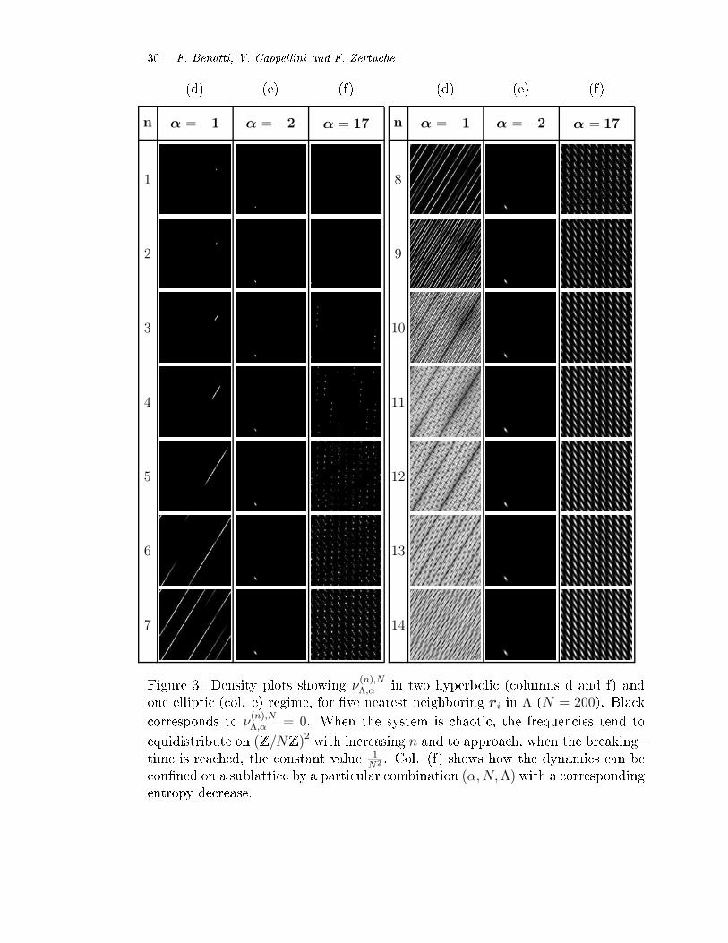
The linear and stationary behaviors of HωN2

(α,Λ, n) are apparent in g. 4,

where four dierent plateaus (2 logN) are rea hed for four dierentN , and in g. 5,

in whi h four dierent slopes are showed for four dierent number of elements in

the partition. With the same parameters as in g. 5, g. 6 shows the orresponding

entropy produ tion hωN2 ,W∞

(α,Λ, n).

5.1.2. Hyperboli regime with D nearest neighbors ri in Λ

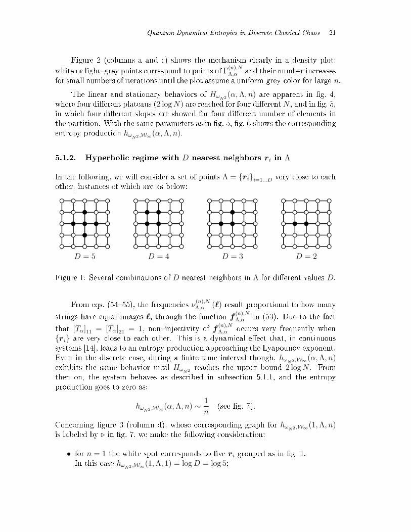
In the following, we will onsider a set of points Λ = rii=1...D very lose to ea h

other, instan es of whi h are as below:

D = 5

D = 4

D = 3

D = 2

Figure 1: Several ombinations of D nearest neighbors in Λ for dierent values D.

From eqs. (5455), the frequen ies ν(n),NΛ,α (ℓ) result proportional to how many

strings have equal images ℓ, through the fun tion f(n),NΛ,α in (53). Due to the fa t

that [Tα]11 = [Tα]21 = 1, noninje tivity of f(n),NΛ,α o urs very frequently when

ri are very lose to ea h other. This is a dynami al ee t that, in ontinuous

systems [14, leads to an entropy produ tion approa hing the Lyapounov exponent.

Even in the dis rete ase, during a nite time interval though, hωN2 ,W∞

(α,Λ, n)exhibits the same behavior until Hω

N2rea hes the upper bound 2 logN . From

then on, the system behaves as des ribed in subse tion 5.1.1, and the entropy

produ tion goes to zero as:

hωN2 ,W∞

(α,Λ, n) ∼ 1

n(see g. 7).

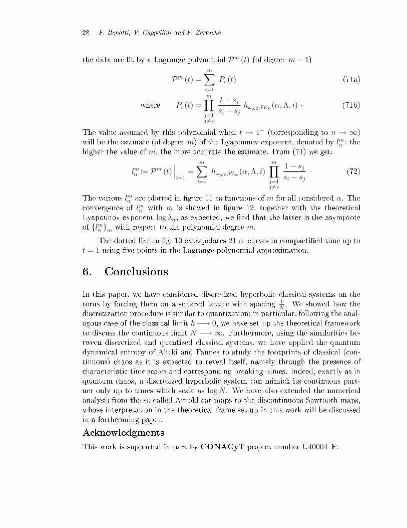
Con erning gure 3 ( olumn d), whose orresponding graph for hωN2 ,W∞

(1,Λ, n)is labeled by ⊲ in g. 7, we make the following onsideration:

• for n = 1 the white spot orresponds to ve ri grouped as in g. 1.

In this ase hωN2 ,W∞

(1,Λ, 1) = logD = log 5;


• for n ∈ [2, 5] the white spot begins to stret h along the stret hing dire tion

of T1. In this ase, the frequen ies ν(n),NΛ,α are not onstant on the lightgrey

region: this leads to a de rease of hωN2 ,W∞

(1,Λ, n);

• for n ∈ [6, 10] the lightgrey region be omes so elongated that it starts feeling

the folding ondition so that, with in reasing timesteps, it eventually fully

overs the originally dark spa e. In this ase, the behavior of hωN2 ,W∞

(1,Λ, n)remains the same as before up to n = 10;

• for n = 11, Γ(n),NΛ,α oin ides with the whole latti e;

• for larger times, the frequen ies ν(n),NΛ,1 tend to the onstant value

1N2 on

almost every point of the grid. In this ase, the behaviour of the entropy

produ tion undergoes a riti al hange (the rossover o urring at n = 11)as showed in g. 7.

Again, we annot on lude that n = 11 is a realisti breakingtime, be ause on e

more we have strong dependen e on the hosen partition (namely from the number

D of its elements). For instan e, in g. 7, one an see that partitions with 3 points

rea h their orresponding breakingtimes faster than that with D = 5; also theydo it in an Ndependent way.

For a hosen set Λ onsisting ofD elements very lose to ea h other and N very

large, hωN2 ,W∞

(α,Λ, n) ≃ log λ (whi h is the asymptote in the ontinuous ase)

from a ertain n up to a time τB. Sin e this latter is now partition independent,

it an properly be onsidered as the breakingtime of the system; it is given by

τB = logλN2· (61)

It is evident from equation (61) that if one knows τBthen also log λ is known. Usually, one is interested

in the latter whi h is a sign of the instability of the

ontinuous lassi al system. In the following we develop

an algorithm whi h allows us to extra t log λ from

studying the orresponding dis retized lassi al system

and its ALFentropy.

In working onditions, N is not large enough to allow for n being smaller than τB;what happens in su h a ase is that Hω

N2 (α,Λ, n) ≃ 2 logN before the asymptote

for hωN2 ,W∞

(α,Λ, n) is rea hed. Given hωN2 ,W∞

(α,Λ, n) for n < τB, it is thus

ne essary to seek means how to estimate the long time behaviour that one would

have if the system were ontinuous.


Remarks 5.1

When estimating Lyapounov exponents from dis retized hyperboli

lassi al systems, by using partitions onsisting of nearest neighbors,

we have to take into a ount some fa ts:

a. hωN2 ,W∞

(α,Λ, n) does not in rease with n; therefore, ifD < λ, hωN2 ,W∞

annot rea h the Lyapounov exponent. Denoted by log λ (D) the

asymptote that we extrapolate from the data

a

, in general we have

λ (D) 6 logD < λ. For instan e, for α = 1, λ = 2.618 . . . > 2 and

partitions with D = 2 annot produ e an entropy greater then log 2;this is the ase for the entropies below the dotted line in gs. 5 e 6;

b. partitions with D small but greater than λ allow log λ to be rea hed

in a very short time and λ (D) is very lose to λ in this ase;

. partitions with D ≫ λ require very long time to onverge to log λ(and so very large N) and, moreover, it is not a trivial task to deal

with them from a omputational point of view. On the ontrary the

entropy behaviour for su h partitions oers very good estimates of λ( ompare, in g. 7, ⊲ with ⋄, , and ) ;

d. in order to ompute λ (and then τB, by (61)), one an al ulate λ (D)for in reasing D, until it onverges to a stable value λ;

e. due to number theoreti al reasons, the UMG on (Z/NZ)2present

several anomalies. An instan e of them is showed in g. 3 ( ol. f),

where a partition with ve nearest neighbors on a latti e of 200×200points onnes the image of f

(n),NΛ,α (under the a tion of a Tα map

with α = 17) on a subgrid of the torus. In this and analogous ases,

there o urs an anomalous depletion of the entropy produ tion and no

signi ant information is obtainable from it. To avoid this di ulties,

in Se tion 5.2 we will go beyond the UMG sub lass onsidered so far.

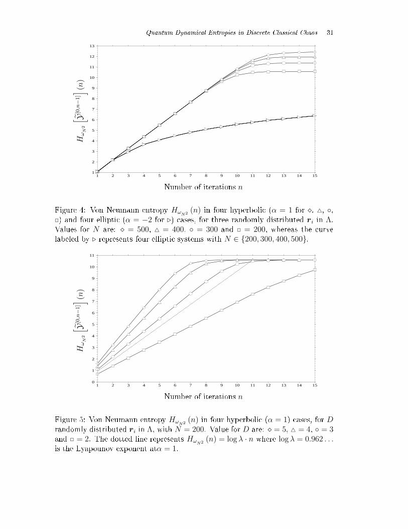
5.1.3. Ellipti regime (α ∈ −1,−2,−3)

One an show that all evolution matri es Tα are hara terized by the following

property:

T 2α = α Tα − 1 , α := (α + 2) · (62)

ahωN2 ,W∞

(α, Λ, n) may even equal log λ (D) from the start.


In the ellipti regime α ∈ −1,−2,−3, therefore α ∈ −1, 0, 1 and relation (62)

determines a periodi evolution with periods:

T 3−1 = −1 (T 6

−1 = 1) (63a)

T 2−2 = −1 (T 4

−2 = 1) (63b)

T 3−3 = +1 · (63 )

It has to be stressed that, in the ellipti regime, the relations (63) do not hold

modulo N, instead they are ompletely independent from N .

Due to the high degree of symmetry in relations (6263), the frequen ies ν(n),NΛ,α

are dierent from zero only on a small subset of the whole latti e.

This behavior is apparent in g. 2 : ol. b, in whi h we onsider ve randomly

distributed ri in Λ, and in g. 3 : ol. e, in whi h the ve ri are grouped as in g. 1.

In both ases, the Von Neumann entropy HωN2 (n) is not linearly in reasing with

n (see gure 8), instead it assumes a logshaped prole ( up to the breakingtime,

see g. 4).

Remark 5.2

The last observation indi ates how the entropy produ tion analysis

an be used to re ognize whether a dynami al systems is hyperboli or

not. If we use randomly distributed points as a partition, we observe

that hyperboli systems show onstant entropy produ tion (up to the

breakingtime), whereas the others do not.

Moreover, unlike hyperboli ones, ellipti systems do not hange their

behaviour with N (for reasonably large N) as learly showed in g. 4,

in whi h ellipti systems (α = −2) with four dierent values of N give

the same plot. On the ontrary, we have dependen e on how ri h is the

hosen partition, similarly to what we have for hyperboli systems, as

showed in g. 7.

5.1.4. Paraboli regime (α ∈ 0, 4)

This regime is hara terized by λ = λ−1 = ±1, that is log |λ | = 0 (see Remark 2.1,

.). These systems behave as the hyperboli ones (see subse tions 5.1.1 and 5.1.2)

and this is true also for the the general behavior of the entropy produ tion, apart

from the fa t that we never fall in the ondition (a.) of Remark 5.1. Then,

for su iently large N , every partition onsisting of D grouped ri will rea h the

asymptote log |λ | = 0.


5.2. The ase of Sawtooth Maps

The Sawtooth Maps [15, 16, are triples (X , µ, Sα) where

X = T

2 = R

2/Z2 = x = (x1, x2) (mod 1) (64a)

Sα

(x1

x2

)=

(1 + α 1α 1

) (〈x1〉x2

)(mod 1) , α ∈ R (64b)

dµ(x) = dx1 dx2 , (64 )

where 〈·〉 denotes the fra tional part of a real number. Without 〈·〉, (64b) is notwell dened on T

2for notinteger α; in fa t, without taking the fra tional part, the

same point x = x+n ∈ T2,n ∈ Z2, would have (in general) Sα (x) 6= Sα (x + n).

Of ourse, 〈·〉 is not ne essary when α ∈ Z.The Lebesgue measure dened in (64 ) is invariant for all α ∈ R.After identifying x with anoni al oordinates (q, p) and imposing the (mod 1) ondition on both of them, the above dynami s an be rewritten as:

q′ = q + p′

p′ = p+ α 〈q〉(mod 1), (65)

This is nothing but the Chirikov Standard Map [4 in whi h − 12π

sin(2πq) is re-

pla ed by 〈q〉. The dynami s in (65) an also be thought of as generated by the

(singular) Hamiltonian

H(q, p, t) =p2

2− α

〈q〉22

δp(t), (66)

where δp(t) is the periodi Dira delta whi h makes the potential a t through

periodi ki ks with period 1.

Sawtooth Maps are invertible and the inverse is given by the expression

S−1α

(x1

x2

)=

(1 0

−α 1

)⟨(1 −10 1

) (x1

x2

)⟩(mod 1) (67)

or, in other words,

q = q′ − p′

p = −α q + p′(mod 1) . (68)

It an indeed be he ked that Sα (S−1α (x)) = S−1

α (Sα (x)) = 〈x〉 , ∀x ∈ T2.

Remarks 5.3


i. Sawtooth Maps Sα are dis ontinuous on the subset

γ0 := x = (0, p) , p ∈ T ∈ T

2: two points lose to this border,

A := (ε, p) and B := (1 − ε, p), have images that dier, in the ε → 0

limit, by a ve tor d(1)

Sα(A,B) = (α, α) (mod 1).

ii. Inverse Sawtooth Maps S−1α are dis ontinuous on the subset

γ−1 := Sα (γ0) = x = (p, p) , p ∈ T ∈ T2: two points lose to this

border, A := (p+ ε, p− ε) and B := (p− ε, p+ ε), have images that

dier, in the ε→ 0 limit, by a ve tor d(1)

S−1α

(A,B) = (0, α) (mod 1).

iii. The hyperboli , ellipti or paraboli behavior of Sawtooth maps is

related to the eigenvalues of ( 1+α 1α 1 ) exa tly as in Remark 2.1.ii.

iv. The Lebesgue measure in (64 ) is S−1α invariant.

From a omputational point of view, the study of the entropy produ tion in the

ase of Sawtooth Maps Sα is more ompli ated than for the Tα's. The reason to

study numeri ally these dynami al systems is twofold:

• to avoid the di ulties des ribed in Remark 5.1 (e.);

• to deal, in a way ompatible with numeri al omputation limits, with the

largest possible spe trum of a essible Lyapounov exponent. We know that

for α ∈ Z⋂ non ellipti domain,

λ± (Tα) = λ± (Sα) =α + 2 ±

√(α + 2)2 − 4

2·

In order to t log λα ( log λα being the Lyapounov exponent orresponding

to a given α) via entropy produ tion analysis, we need D elements in the

partition (see points b. and . of Remark 5.1) with D > λα. Moreover,

if we were to study the power of our method for dierent integer values of

α we would be for ed for ed to use very large D, in whi h ase we would

need very long omputing times in order to evaluate numeri ally the entropy

produ tion hωN2 ,W∞

(α,Λ, n) in a reasonable interval of times n. Instead,

for Sawtooth Maps, we an x the parameters (N,D,Λ) and study λα for

α onned in a small domain, but free to assume every real value in that

domain.

In the following, we investigate the ase of α in the hyperboli regime with Dnearest neighbors ri in Λ, as done in subse tion 5.1.2. In parti ular, gures (912)

refer to the following xed parameters:


N = 38 ; nmax

= 5 ; D = 5 ;

Λ : r1 =

(78

), r2 =

(79

), r3 =

(68

), r4 =

(77

), r5 =

(88

);

α : from 0.00 to 1.00 with an in remental step of 0.05.

First, we ompute the Von Neumann entropy (49) using the (hermitian) matrix

Gℓ1,ℓ2 (n) dened in (48). This is a tually a diagonalization problem: on e that

the N2eigenvalues ηiN

2

i=1 are found, then

HωN2

[Y [0,n−1]

]= −

N2∑

i=1

ηi log ηi · (69)

Then, from (59), we an determine hωN2 ,W∞

(α,Λ, n). In the numeri al example,

the (Λdependent) breakingtime o urs after n = 5; for this reason we have

hosen nmax

= 5. In fa t, we are interested in the region where the dis rete system

behaves almost as a ontinuous one.

In gure 9, the entropy produ tion is plotted for the hosen set of α's: for verylarge N (that is lose to the ontinuum limit, in whi h no breakingtime o urs)

all urves ( hara terized by dierent α's) would tend to log λα with n.

One way to determine the asymptote log λα is to t the de reasing fun tion

hωN2 ,W∞

(α,Λ, n) over the range of data and extrapolate the t for n → ∞. Of

ourse we an not perform the t with polynomials, be ause every polynomial

diverges in the n→ ∞ limit.

A better strategy is to ompa tify the time evolution by means of a isomorphi

positive fun tion s with bounded range, for instan e:

N ∋ n 7−→ sn :=2

πarctan (n− 1) ∈ [0, 1] · (70)

Then, for xed α, in g. 10 we onsider nmax

points

(sn , hω

N2 ,W∞(α,Λ, n)

)and

extra t the asymptoti value of hωN2 ,W∞

(α,Λ, n) for n → ∞, that is the value of

hωN2 ,W∞

(α,Λ, s−1 (t)

)for t→ 1−, as follows.

Given a graph onsisting of m ∈ 2, 3, · · · , nmax

points, in our ase the rst

m points of urves as in g. 10, namely

(s1 , hω

N2 ,W∞(α,Λ, 1)

),(s2 , hω

N2 ,W∞(α,Λ, 2)

), · · · ,

(sm , hω

N2 ,W∞(α,Λ, m)

),


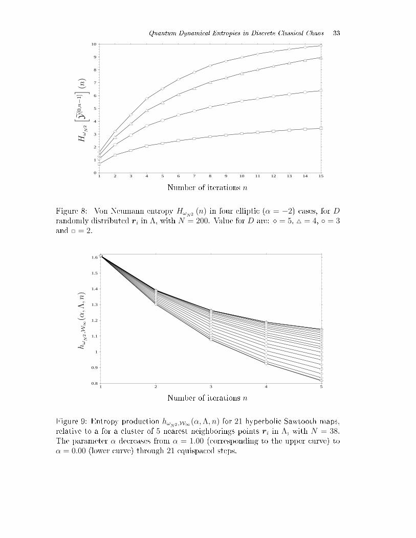
the data are t by a Lagrange polynomial Pm (t) (of degree m− 1)

Pm (t) =m∑

i=1

Pi (t) (71a)

where Pi (t) =

m∏

j=1j 6= i

t− sjsi − sj

hωN2 ,W∞

(α,Λ, i) · (71b)

The value assumed by this polynomial when t → 1− ( orresponding to n → ∞)

will be the estimate (of degree m) of the Lyapounov exponent, denoted by lmα : thehigher the value of m, the more a urate the estimate. From (71) we get:

lmα := Pm (t)∣∣∣t=1

=m∑

i=1

hωN2 ,W∞

(α,Λ, i)m∏

j=1j 6= i

1 − sjsi − sj

· (72)

The various lmα are plotted in gure 11 as fun tions of m for all onsidered α. The onvergen e of lmα with m is showed in gure 12, together with the theoreti al

Lyapounov exponent log λα; as expe ted, we nd that the latter is the asymptote

of lmα m with respe t to the polynomial degree m.

The dotted line in g. 10 extrapolates 21 α urves in ompa tied time up to

t = 1 using ve points in the Lagrange polynomial approximation.

6. Con lusions

In this paper, we have onsidered dis retized hyperboli lassi al systems on the

torus by for ing them on a squared latti e with spa ing

1N. We showed how the

dis retization pro edure is similar to quantization; in parti ular, following the anal-

ogous ase of the lassi al limit ~ 7−→ 0, we have set up the theoreti al framework

to dis uss the ontinuous limit N 7−→ ∞. Furthermore, using the similarities be-

tween dis retized and quantized lassi al systems, we have applied the quantum

dynami al entropy of Ali ki and Fannes to study the footprints of lassi al ( on-

tinuous) haos as it is expe ted to reveal itself, namely through the presen e of

hara teristi time s ales and orresponding breakingtimes. Indeed, exa tly as in

quantum haos, a dis retized hyperboli system an mimi k its ontinuous part-

ner only up to times whi h s ale as logN . We have also extended the numeri al

analysis from the so alled Arnold at maps to the dis ontinuous Sawtooth maps,

whose interpretation in the theoreti al frame set up in this work will be dis ussed

in a forth oming paper.

A knowledgments

This work is supported in part by CONACyT proje t number U40004F.


n α = 1 α = −2 α = 17

(a) (b) ( )

n α = 1 α = −2 α = 17

(a) (b) ( )

1

2

3

4

5

6

7

8

9

10

11

12

13

14

Figure 2: Density plots showing the frequen ies ν(n),NΛ,α in two hyperboli regimes

( olumns a and ) and an ellipti one ( ol. b), for ve randomly distributed ri in

Λ with N = 200. Bla k orresponds to ν(n),NΛ,α = 0. In the hyperboli ases, ν

(n),NΛ,α

tends to equidistribute on (Z/NZ)2with in reasing n and be omes onstant when

the breakingtime is rea hed.


n α = 1 α = −2 α = 17

(d) (e) (f)

n α = 1 α = −2 α = 17

(d) (e) (f)

1

2

3

4

5

6

7

8

9

10

11

12

13

14

Figure 3: Density plots showing ν(n),NΛ,α in two hyperboli ( olumns d and f) and

one ellipti ( ol. e) regime, for ve nearest neighboring ri in Λ (N = 200). Bla k

orresponds to ν(n),NΛ,α = 0. When the system is haoti , the frequen ies tend to

equidistribute on (Z/NZ)2with in reasing n and to approa h, when the breaking

time is rea hed, the onstant value

1N2 . Col. (f) shows how the dynami s an be

onned on a sublatti e by a parti ular ombination (α,N,Λ) with a orrespondingentropy de rease.


1 2 3 4 5 6 7 8 9 10 11 12 13 14 151

2

3

4

5

6

7

8

9

10

11

12

13

Hω

N2

[ Y[0,n−

1]] (n

)

Number of iterations n

Figure 4: Von Neumann entropy HωN2

(n) in four hyperboli (α = 1 for ⋄, , ,) and four ellipti (α = −2 for ⊲) ases, for three randomly distributed ri in Λ.Values for N are: ⋄ = 500, = 400, = 300 and = 200, whereas the urve

labeled by ⊲ represents four ellipti systems with N ∈ 200, 300, 400, 500.

1 2 3 4 5 6 7 8 9 10 11 12 13 14 150

1

2

3

4

5

6

7

8

9

10

11

Hω

N2

[ Y[0,n−

1]] (n

)


Figure 5: Von Neumann entropy HωN2

(n) in four hyperboli (α = 1) ases, for Drandomly distributed ri in Λ, with N = 200. Value for D are: ⋄ = 5, = 4, = 3and = 2. The dotted line represents Hω

N2(n) = log λ · n where log λ = 0.962 . . .

is the Lyapounov exponent atα = 1.


1 2 3 4 5 6 7 8 9 10 11 12 13 14 150.6

0.7

0.8

0.9

1

1.1

1.2

1.3

1.4

1.5

1.6

1.7

hω

N2,W

∞(α,Λ,n

)


Figure 6: Entropy produ tion hωN2 ,W∞

(α,Λ, n) in four hyperboli (α = 1) ases,for D randomly distributed ri in Λ, with N = 200. Values for D are: ⋄ = 5, = 4, = 3 and = 2. The dotted line orresponds to the Lyapounov exponent

log λ = 0.962 . . . at α = 1.

1 2 3 4 5 6 7 8 9 10 11 12 13 140.6

0.7

0.8

0.9

1

1.1

1.2

1.3

1.4

1.5

1.6

1.7

hω

N2,W

∞(α,Λ,n

)



(α,Λ, n) in ve hyperboli (α = 1) ases,for D nearest neighboring points ri in Λ. Values for (N,D) are: ⊲ = (200, 5), ⋄ =(500, 3), = (400, 3), = (300, 3) and = (200, 3). The dotted line orresponds

to the Lyapounov exponent log λ = 0.962 . . . at α = 1 and represents the natural

asymptote for all these urves in absen e of breakingtime.


1 2 3 4 5 6 7 8 9 10 11 12 13 14 150

1

2

3

4

5

6

7

8

9

10

Hω

N2

[ Y[0,n−

1]] (n

)


Figure 8: Von Neumann entropy HωN2 (n) in four ellipti (α = −2) ases, for D

randomly distributed ri in Λ, with N = 200. Value for D are: ⋄ = 5, = 4, = 3and = 2.

1 2 3 4 50.8

0.9

1

1.1

1.2

1.3

1.4

1.5

1.6

hω

N2,W

∞(α,Λ,n

)



(α,Λ, n) for 21 hyperboli Sawtooth maps,

relative to a for a luster of 5 nearest neighborings points ri in Λ, with N = 38.The parameter α de reases from α = 1.00 ( orresponding to the upper urve) to

α = 0.00 (lower urve) through 21 equispa ed steps.


0 0.1 0.2 0.3 0.4 0.5 0.6 0.7 0.8 0.9 10.2

0.3

0.4

0.5

0.6

0.7

0.8

0.9

1

1.1

1.2

1.3

1.4

1.5

1.6

hω

N2,W

∞

( α,Λ,s

−1(t

))

Compa tied time t

Figure 10: The solid lines orrespond to

(sn , hω

N2 ,W∞(α,Λ, n)

), with n ∈

1, 2, 3, 4, 5, for the values of α onsidered in gure 9. Every α urve is on-

tinued as a dotted line up to (1, l5α), where l5α is the Lyapounov exponent extra ted

from the urve by tting all the ve points via a Lagrange polynomial Pm (t).

2 3 4 50.2

0.3

0.4

0.5

0.6

0.7

0.8

0.9

1

1.1

1.2

A

p

p

r

o

x

i

m

a

t

e

d

L

y

a

p

o

u

n

o

v

e

x

p

o

n

e

n

t

lm α

Degree of a ura y m

Figure 11: Four estimated Lyapounov exponents lmα plotted vs. their degree of

a ura y m for the values of α onsidered in gures 9 and 10.


0 0.1 0.2 0.3 0.4 0.5 0.6 0.7 0.8 0.9 10

0.1

0.2

0.3

0.4

0.5

0.6

0.7

0.8

0.9

1

1.1

1.2

A

p

p

r

o

x

i

m

a

t

e

d

L

y

a

p

o

u

n

o

v

e

x

p

o

n

e

n

t

lm α

Hyperboli ity parameter α

Figure 12: Plots of the four estimated of Lyapounov exponents lmα of gure 11

vs. the onsidered values of α. The polynomial degree m is as follows: ⋄ = 2, = 3, = 4 and = 5. The solid line orresponds to the theoreti al Lyapounov

exponent log λα = log (α + 2 +√α (α + 4) ) − log 2.


Referen es

[1 Devaney R. An Introdu tion to Chaoti Dynami al Systems, Addison Wesley

Publ. Co. Reading MA, (1989).

[2 Wiggins, S. Dynami al Systems and Chaos. Springer-Verlag. New York (1990).

[3 Katok A. and Hasselblatt B. Introdu tion to the Modern Theory of Dynami al

Systems. Cambridge University Press. Cambridge (1999).

[4 Casati G., Chirikov B. Quantum Chaos. Between Order and Disorder. Cam-

bridge University Press. Cambridge (1995)

[5 Crisanti A., Fal ioni M. and Vulpiani A. Transition from Regular to Complex

Behavior in a Dis rete Deterministi Asymmetri Neural Network Model. J.

Phys. A: Math. Gen. 26 (1993) 3441.

[6 Crisanti A., Fal ioni M., Manti a G. and Vulpiani A. Applying Algorithmi

Complexity to Dene Chaos in the Motion of Complex Systems. Phys. Rev. E

50 (1994) 1959-1967.

[7 Boetta G., Cen ini M., Fal ioni M. and Vulpiani A. Predi tability: a way to

hara terize Complexity. nlin.CD/0101029.

[8 Zertu he F., López-Peña R. and Waelbroe k H. Re ognition of Temporal Se-

quen es of Patterns with State-Dependent Synapses. J. Phys. A: Math. Gen.

27 (1994) 5879-5887.

[9 Zertu he F. and Waelbroe k H. Dis rete Chaos. J. Phys. A: Math. Gen. 32

(1999) 175-189.

[10 Alekseev V. M., Yakobson M. V. Symboli Dynami s and Hyperboli Dynam-

i al Systems. Phys. Rep. 75 (1981) 287-325.

[11 Fal ioni M., Manti a G., Pigolotti S. and Vulpiani A. Coarse-grained prob-

abilisti automata mimi king haoti systems. Phys. Rev. Lett. 91 (2003)

044101.

[12 Ali ki R. and Fannes M. Dening Quantum Dynami al Entropy. Lett. Math.

Phys. 32 (1994) 75-82.

[13 Ali ki R. and Fannes M. Quantum Dynami al Systems. Oxford University

Press (2001).

[14 R. Ali ki, J. Andries, M. Fannes & P. Tuyls, An Algebrai Approa h to the

KolmogorovSinai Entropy, Rev. Math. Phys. 8 (1996) 167

http://arxiv.org/abs/nlin/0101029


[15 N. Cherno, Ergodi and statisti al properties of pie ewise linear hyperboli

automorphisms of the two-torus, J.Stat.Phys. 69 (1992), 111-134.

[16 S. Vaienti, Ergodi properties of the dis ontinuous sawtooth map, J. Stat. Phys.

67, (1992), 251.

[17 I. C. Per ival and F. Vivaldi, A linear ode for the sawtooth and at maps

Physi a D 27 (1987) 373.

[18 S. De Bièvre, Chaos, Quantization and the Classi al Limit on the Torus,

Pro eedings of the XIVth Workshop on Geometri al Methods in Physi s,

Bialowieza, (1995), mp_ar 96191, Polish S ienti Publisher PWN (1998)

[19 S. De Bièvre, Quantum haos: a brief rst visit, Contemporary Mathemati s

289 (2001) 161

[20 Reed M. and Simon B. Methods of Modern Mathemati al Physi s. I: Fun -

tional analysis. A ademi Press. New York (1972).

[21 H. Araki and E. H. Lieb, Entropy Inequalities, Comm. Math. Phys., 18 (1970)

160170

Quantum dynamical entropies in discrete classical chaos

Documents

Transcript of Quantum dynamical entropies in discrete classical chaos