arX

iv:h

ep-t

h/04

0606

6v1

7 J

un 2

004

Chaos in the thermodynamic Bethe ansatzCity CMS 0304/LPENSL-TH-04

Chaos in the thermodynamic Bethe ansatz

Olalla Castro-Alvaredo◦ and Andreas Fring•

◦ Laboratoire de Physique, Ecole Normale Superieure de Lyon,

46 Allee d’Italie, 69364 Lyon CEDEX, France

E-mail: ocastroa@ens-lyon.fr• Centre for Mathematical Science, City University,

Northampton Square, London EC1V 0HB, UK

E-mail: A.Fring@city.ac.uk

Abstract: We investigate the discretized version of the thermodynamic Bethe ansatz

equation for a variety of 1+1 dimensional quantum field theories. By computing Lyapunov

exponents we establish that many systems of this type exhibit chaotic behaviour, in the

sense that their orbits through fixed points are extremely sensitive with regard to the

initial conditions.

1. Introduction

The thermodynamic Bethe ansatz (TBA) equation [1, 2] is an important tool in the context

of 1+1 dimensional integrable quantum field theories. It serves to extract various types of

informations, such as the Virasoro central charge of the underlying ultraviolet conformal

field theory [3], vacuum expectation values [1, 4] etc. As it is a nonlinear integral equation,

it can be solved analytically only in very few circumstances. In general, one relies on

numerical solutions of its discretised version

εn+1A (θ) = rmA cosh θ −

∑

B

∞∫

−∞

dθ′ϕAB(θ − θ′) ln(

1 + e−εnB

(θ′))

. (1.1)

Here r is the inverse temperature, mA is the mass of a particle of type A, θ is the rapidity

and ϕAB denotes the logarithmic derivative of the scattering matrix between the particles

of type A and B. The unknown quantities in these equations are the pseudo-energies

εA(θ). The standard solution procedure for (1.1) consists of a consecutive iteration of the

equation with initial values ε0A(θ) = rmA cosh θ. At the heart of this procedure lie the

assumptions that the exact solution is reached for n → ∞, i.e. the sequence converges, and

furthermore that the final answer is non-sensitive with regard to the initial values, that

is its uniqueness. In general these assumptions are poorly justified and only few rigorous

investigations for some simple models exist [5, 2, 6]. So far the outcome has always been

Chaos in the thermodynamic Bethe ansatz

that these assumptions on the existence and uniqueness of the solution indeed hold, albeit

for certain systems convergence problems in certain regimes have been noted [7, 8]. The

main purpose of this note is to show that this believe has to be challenged and is in fact

unjustified for certain well defined theories. We note that our findings do neither effect the

principles of the TBA itself nor the consistency of the quantum field theory it is meant

to investigate. However, they indicate that one needs to be very cautious when using the

above solution procedure and making deductions about the physics for such theories as one

might just be mislead by the non-convergence of the mathematical procedure used to solve

the TBA-equations.

Here we will not analyze the full TBA-equations (1.1), but rather concentrate on

the ultraviolet regime, that is r ≈ 0, in which it possess some approximation. Clearly,

the occurrence of chaotic behaviour in this regime will have consequences for the finite

temperature regime. We encounter the interesting phenomenon that the iterative procedure

is convergent beyond the ultraviolet (or for a certain choice of parameters in some theories),

but that unstable fixed points are present in the ultraviolet, meaning that this regime can

never be reached by the iterative solution procedure for (1.1).

2. Stability of fixed points and Lyapunov exponents

For completeness, let us first briefly recall a few well known basic facts concerning the

nature of fixed points which may be found in standard text books on dynamical systems,

see e.g. [9]. The objects of our investigations are difference equations of the type

~xn+1 = ~F (~xn), (2.1)

where n ∈ N0, ~xn ∈ Rℓ and ~F : R

ℓ → Rℓ is a vector function. We are especially interested

in the fixed points ~xf of this system being defined as

~F (~xf ) = ~xf . (2.2)

The fixed point is reached by iterating (2.1), if for a perturbation of it, defined as ~yn =

~xn − ~xf , we have limn→∞ ~yn = 0. From (2.1) we find

~yn+1 + ~xf = ~F (~yn + ~xf ) = ~F (~xf ) + J · ~yn + O(|~yn|2) for ~yn → 0 (2.3)

where J is the ℓ × ℓ Jacobian matrix of the vector function ~F (~x)

Jij =∂Fi

∂xj

∣

∣

∣

∣

~xf

for 1 ≤ i, j ≤ ℓ. (2.4)

The linearized system which arises from (2.3) for ~yn → 0

~yn+1 = J · ~yn (2.5)

governs the nature of the fixed point under certain conditions [9]. Evidently, it is solved

by

~yn = qni ~vi with J · ~vi = qn

i ~vi for 1 ≤ i ≤ ℓ . (2.6)

– 2 –

Chaos in the thermodynamic Bethe ansatz

Excluding the case when the eigenvectors ~vi of the Jacobian matrix are not linearly inde-

pendent, we can expand the initial value uniquely

~y0 =ℓ∑

i=1

ςi~vi (2.7)

such that

~yn =

ℓ∑

i=1

ς iqni ~vi . (2.8)

It is now obvious from (2.8) that the perturbation of the fixed point ~yn will grow for

increasing n if |qi| > 1 for some i ∈ {1, . . . , ℓ}. In that case the fixed point ~xf is said to

be linearly unstable. On the other hand, if |qi| < 1 for all i ∈ {1, . . . , ℓ} the perturbation

will tend to zero for increasing n and the fixed point ~xf is said to be linearly stable. It can

be shown that under some conditions [9] the fixed points are nonlinearly stable when they

are linearly stable.

In general, that is for any point ~x rather than just the fixed points ~xf , stability prop-

erties are easily encoded in the Lyapunov exponents λi. Roughly speaking the Lyapunov

exponents are a measure for the exponential separation of neighbouring orbits. One speaks

of unstable (chaotic) orbits if λi > 0 for some i ∈ {1, . . . , ℓ} and stable orbits if λi < 0

for all i ∈ {1, . . . , ℓ}. For an arbitrary point ~x the ℓ Lyapunov exponents for the above

mentioned system (2.1) are defined as

λi = limn→∞

[

1

nln∣

∣

∣qi[~F

n(~x)]∣

∣

∣

]

= limn→∞

[

1

n

n−1∑

k=0

ln∣

∣

∣qi[~F

k(~x)]∣

∣

∣

]

, (2.9)

where the qi (~x) are the eigenvalues of the Jacobian matrix as defined in (2.6), but now at

some arbitrary point ~x. Taking the point to be a fixed point, we can relate (2.9) to the

above statements. At the fixed point we have of course ~F k(~xf ) = ~xf , such that

λi = limn→∞

[

1

n

n−1∑

k=0

ln |qi (~xf )|]

= ln |qi| . (2.10)

Therefore, a stable fixed point is characterized by λi < 0 or |qi| < 1 for all i ∈ {1, . . . , ℓ}and an unstable fixed point by λi > 0 or |qi| > 1 for some i ∈ {1, . . . , ℓ}. We can now

employ this criterion for some concrete systems.

3. Unstable fixed points in constant TBA equations

We adopt here the notation of [10, 11, 12], by which a large class of integrable quantum

field theories can be referred to in a general Lie algebraic form as g|g-theories. Their

underlying ultraviolet conformal field theories can be described by the theories investigated

in [13, 14, 15] (and special cases thereof) with Virasoro central charge c = ℓℓh/(h+h). Here

ℓ(ℓ) and h(h) are the rank and the Coxeter number of g(g), respectively. In particular,

g|A1 is identical to the minimal affine Toda theories (ATFT) [16, 17] and An|g corresponds

– 3 –

Chaos in the thermodynamic Bethe ansatz

to the gn+1-homogeneous Sine-Gordon (HSG) models [18, 19]. In this formulation each

particle is labelled by two quantum numbers (a, i), which take their values in 1 ≤ a ≤ ℓ and

1 ≤ i ≤ ℓ. Hence, in total we have ℓ× ℓ different particle types. It is a standard procedure

in this context [1, 2] to approximate the pseudo-energies in (1.1) by εia(θ) = εi

a = const

in a large region for θ when r is small. For convenience one then introduces further the

quantity xia = exp(−εi

a) such that (1.1) can be cast into the compact form

xia =

ℓ∏

b=1

ℓ∏

j=1

(1 + xjb)

N ij

ab =: F ia(~x) with N ij

ab = δabδij − K−1ab Kij . (3.1)

The matrix N ijab in (3.1) encodes the information on the asymptotic behaviour of the scat-

tering matrix. As stated in (3.1) it is specific to each of the g|g-theories with K and K

being the Cartan matrix of g and g, respectively. The equations (3.1) are referred to as the

constant TBA-equations. They govern the ultraviolet behaviour of the system and their

solutions yield directly the effective central charge

ceff =6

π2

ℓ∑

a=1

ℓ∑

i=1

L(

xia

1 + xia

)

(3.2)

with L(x) =∑

∞

n=1 xn/n2 + ln x ln(1 − x)/2 denoting Rogers dilogarithm (see e.g. [20] for

properties).

Let us now discretise (3.1) and analyze it with regard to the nature of its fixed points.

According to the argument of section 2, we have to compute first of all the Jacobian

matrices of ~F

J ijab =

∂F ia

∂xjb

∣

∣

∣

∣

∣

~xf

= N ijab

(

xia

)

f

1 + (xjb)f

. (3.3)

Next we need to determine the eigensystem of the Jacobian matrix. This is not possible to

do in a completely generic way at present, since not even the solutions, i.e. fixed points,

of (3.1) are known in a general fashion. Instead, we present some examples to exhibit the

possible types of behaviour.

3.1 Stable fixed points

We start with a simple example of a stable fixed point. We present the A2|A1 case, which

after the free Fermion (A1|A1) is the next non-trivial example in the series of the minimal

ATFTs, the scaling three-state Potts model with Virasoro central charge c = 4/5. The

TBA has been investigated in [1, 2]. The constant TBA-equations (3.1)

x1 = (1 + x1)−1/3(1 + x2)

−2/3 = F1(~x), x2 = (1 + x1)−2/3(1 + x2)

−1/3 = F2(~x), (3.4)

can be solved analytically by the golden ratio τ := (√

5 − 1)/2 = x1 = x2. Using this

solution for the fixed point ~xf = (x1, x2), we compute the Jacobian matrix of ~F (~x)

J(~xf ) = −1

3

(

τ2 2τ2

2τ 2 τ2

)

, (3.5)

– 4 –

Chaos in the thermodynamic Bethe ansatz

with eigensystem

q1 = −τ2 ≈ −0.38197, ~v1 = (1, 1), q2 = τ2/3 ≈ 0.12732, ~v2 = (−1, 1) .

As the eigenvectors are obviously linearly independent and |q1| < 1, |q2| < 1, we deduce that

all Lyapunov exponents are negative and therefore that the fixed point is stable. Indeed,

numerical studies of this system exhibit a fast convergence and a non-sensitive behaviour

with regard to the initial values of the iterative procedure.

For some theories the solutions are known analytically in a closed form. For instance,

the constant TBA equations for the A1|Aℓ-theories (≡ SU(ℓ + 1)2-HSG-model) are solved

by

xi1 =

[

sin[π(1 + i)λ]

sin(πλ)

]2

− 1, for 1 ≤ i ≤ ℓ (3.6)

with λ = 1/(3+ ℓ) [21, 22, 23, 12]. Taking this solution for the fixed point we compute the

Jacobian matrix (3.3) with Nij = (δi,j+1 + δi,j−1)/2 to

J ij11(~xf ) =

1

2

[

sin[π(2 + i)λ]

sin(iπλ)δi,j+1 +

sin(iπλ)

sin[π(2 + i)λ]δi,j−1

]

. (3.7)

and the eigenvalues to qi = cos[π(i + 1)λ]. As |qi| < 1 for all i ∈ {1, . . . , ℓ} the fixed points

are stable. We investigated various minimal affine Toda field theories which all posses fixed

points of this nature. In fact, the general assumption is that all systems exhibit such a

behaviour. We present now some counter examples which refute this believe.

3.2 Stable two-cycles

We start with a system which does not possess a stable fixed point, but rather a stable

two-cycle, i.e. a solution for~G(~x) := ~F (~F (~x)) = ~x . (3.8)

We consider the A2|A2-theories (≡ SU(3)3-HSG model) studied already previously by

means of the TBA in [24]. Its extreme ultraviolet Virasoro central charge is c = 2. The

constant TBA-equations for this case read

x11 =

(1 + x21)

2/3(1 + x22)

1/3

(1 + x11)

1/3(1 + x12)

2/3= F1(~x), x1

2 =(1 + x2

1)1/3(1 + x2

2)2/3

(1 + x11)

2/3(1 + x12)

1/3= F2(~x), (3.9)

x21 =

(1 + x11)

2/3(1 + x12)

1/3

(1 + x21)

1/3(1 + x22)

2/3= F3(~x), x2

2 =(1 + x1

1)1/3(1 + x1

2)2/3

(1 + x21)

2/3(1 + x22)

1/3= F4(~x), (3.10)

with analytic solution x11 = x1

2 = x21 = x2

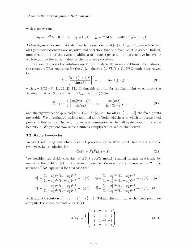
2 = 1. Taking this solution as the fixed point, we

compute the Jacobian matrix for ~F (~x)

J(~xf ) =1

6

−1 −2 2 1

−2 −1 1 2

2 1 −1 −2

1 2 −2 −1

(3.11)

– 5 –

Chaos in the thermodynamic Bethe ansatz

with eigensystem

q1 = −1, ~v1 = (−1,−1, 1, 1), q2 = 1/3, ~v2 = (−1, 1,−1, 1),

q3 = 0, ~v3 = (1, 0, 0, 1), q4 = 0, ~v4 = (0, 1, 1, 0).(3.12)

We observe that there is one eigenvalue with |q1| = 1, which is generally called a marginal

behaviour, i.e. the stability properties depend on the other eigenvalues and on the next

leading order. In fact, we can see from (2.8) that the perturbation of the fixed point will

remain the same even for large values of n, flipping between two values and thus suggesting

the existence of a stable two cycle (3.8). We find that (3.8) can be solved by

x11 = x1

2 = 1/x21 = 1/x2

2 = κ, (3.13)

for any arbitrary value of κ. To determine the stability of the two-cycle we have to compute

the Jacobian matrix for G(~x)

J(~xf ) =1

9 + 9κ

5κ 4κ −4κ2 −5κ2

4κ 5κ −5κ2 −4κ2

−4/κ −5/κ 5 4

−5/κ −4/κ 4 5

(3.14)

which has eigensystem

q1 = 1, ~v1 = (−κ2,−κ2, 1, 1) q2 = 1/9, ~v2 = (−κ2, κ2,−1, 1),

q3 = 0, ~v3 = (κ, 0, 0, 1), q4 = 0, ~v4 = (0, κ, 1, 0).(3.15)

We conclude from this that one approaches a stable two-cycle when iterating the discretised

version of (3.8). Thus, we note that the TBA-system for the SU(3)3-HSG model in the

ultraviolet regime does not posses a stable fixed point but an infinite number of stable

two-cycles of the type (3.13). It is now intriguing to note that when using this solution

to compute the effective Virasoro central charge (3.2), one always obtains the expected

value c = 2 for any value of κ ∈ R, simply due to an identity for the Rogers dilogarithm

L(1 − x) + L(x) = π2/6. Hence, despite the fact, that one is using entirely wrong pseudo-

energies, one obtains by pure luck an apparent confirmation of the theories consistency.

3.3 Unstable fixed points, chaotic behaviour

In this section we present some TBA-systems for well-defined quantum field theories, which

exhibit a chaotic behaviour in the sense that their iterative solutions are extremely sensitive

with regard to the initial values.

3.3.1 A4|A4

This model is the SU(5)5-HSG model with extreme ultraviolet Virasoro central charge

c = 8. To reduce the complexity of the model, we exploit already from the very beginning

the Z2-symmetries in the A4-Dynkin diagrams and identify x11 = x4

1 = x14 = x4

4, x22 = x3

2 =

– 6 –

Chaos in the thermodynamic Bethe ansatz

x23 = x3

3, x12 = x1

3 = x42 = x4

3, x21 = x2

4 = x31 = x3

4. With these identifications the constant

TBA-equations can be brought into the form

x11 =

(1 + x21)(1 + x2

2)

(1 + x11)(1 + x1

2)2

= F1(~x), x12 =

(1 + x21)(1 + x2

2)2

(1 + x11)

2(1 + x12)

3= F2(~x), (3.16)

x21 =

(1 + x11)(1 + x1

2)

(1 + x22)

= F3(~x), x22 =

(1 + x11)

2(1 + x12)

2

(1 + x21)(1 + x2

2)= F4(~x). (3.17)

We can solve these equations analytically by one, τ and τ := 1/τ = (√

5 + 1)/2

x11 = x4

1 = x14 = x4

4 = x22 = x3

2 = x23 = x3

3 = 1,

x21 = x2

4 = x31 = x3

4 = τ , (3.18)

x12 = x1

3 = x42 = x4

3 = τ .

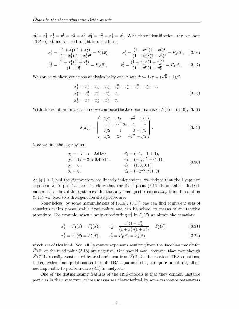
With this solution for ~xf at hand we compute the Jacobian matrix of ~F (~x) in (3.16), (3.17)

J(~xf ) =

−1/2 −2τ τ2 1/2

−τ −3τ2 2τ − 1 τ

τ/2 1 0 −τ/2

1/2 2τ −τ2 −1/2

. (3.19)

Now we find the eigensystem

q1 = −τ2 ≈ −2.6180, ~v1 = (−1,−1, 1, 1),

q2 = 4τ − 2 ≈ 0.47214, ~v2 = (−1, τ 2,−τ2, 1),

q3 = 0, ~v3 = (1, 0, 0, 1),

q4 = 0, ~v4 = (−2τ 2, τ , 1, 0).

(3.20)

As |q1| > 1 and the eigenvectors are linearly independent, we deduce that the Lyapunov

exponent λ1 is positive and therefore that the fixed point (3.18) is unstable. Indeed,

numerical studies of this system exhibit that any small perturbation away from the solution

(3.18) will lead to a divergent iterative procedure.

Nonetheless, by some manipulations of (3.16), (3.17) one can find equivalent sets of

equations which posses stable fixed points and can be solved by means of an iterative

procedure. For example, when simply substituting x11 in F2(~x) we obtain the equations

x11 = F1(~x) = F ′

1(~x), x12 =

x11(1 + x2

2)

(1 + x11)(1 + x1

2)= F ′

2(~x), (3.21)

x21 = F3(~x) = F ′

3(~x), x22 = F4(~x) = F ′

4(~x), (3.22)

which are of this kind. Now all Lyapunov exponents resulting from the Jacobian matrix for~F ′(~x) at the fixed point (3.18) are negative. One should note, however, that even though~F ′(~x) it is easily constructed by trial and error from ~F (~x) for the constant TBA-equations,

the equivalent manipulations on the full TBA-equations (1.1) are quite unnatural, albeit

not impossible to perform once (3.1) is analyzed.

One of the distinguishing features of the HSG-models is that they contain unstable

particles in their spectrum, whose masses are characterized by some resonance parameters

– 7 –

Chaos in the thermodynamic Bethe ansatz

σij with 1 ≤ i, j ≤ ℓ. We can now interpret these parameters as bifurcation parameters as

common in the study of chaotic systems and investigate the nature of the fixed points when

these parameters are varied. In [7] a precise decoupling rule was provided, which describes

the behaviour of the theories when some of the σ′s become large and tend to infinity. For

SU(5)5 we have for instance the following possibilities

limσ12→∞

SU(5)5 = SU(2)5 ⊗ SU(4)5 or limσ23→∞

SU(5)5 = SU(3)5 ⊗ SU(3)5 . (3.23)

For the algebras involved we found that the fixed point of SU(4)5 is unstable, whereas the

fixed points of SU(3)5 and SU(2)5 are stable. For our SU(5)5 example this implies that the

fixed point in SU(3)5 ⊗SU(3)5 will be stable, whereas the fixed point in SU(2)5 ⊗SU(4)5will be unstable. In general, we find that, while approaching the ultraviolet from the

infrared, once the nature of the fixed point has changed from stable to unstable it remains

that way. This behaviour can be encoded naturally in standard bifurcation diagrams, which

we present elsewhere.

We also found unstable fixed points for other HSG-models related to simply laced

algebras and g|g-theories which are neither HSG nor minimal ATFT. A priori the behaviour

is difficult to predict, e.g. whereas D4|D4 (see [10] for the solution of (3.1) ) and D4|A4

have unstable fixed points, the fixed point in D4|A2 is stable.

3.3.2 A1|C2

This model is the simplest example of an HSG model related to a non-simply laced algebra,

namely the Sp(4)2-HSG model with central charge c = 2. In the TBA analysis carried out

in [7] convergence problems in the ultraviolet regime were already commented upon. In

fact, we find here that all HSG models which are related to non-simply laced Lie algebras

posses unstable fixed points. The constant TBA-equations for A1|C2 read

x11 =

√

(1 + x21)(1 + x2

3)(1 + x22) = F1(~x), x2

1 =1

(1 + x22)

√

(1 + x11)

(1 + x21)(1 + x2

3)= F2(~x),(3.24)

x22 =

(1 + x11)

(1 + x21)(1 + x2

2)(1 + x23)

= F3(~x), x23 =

1

(1 + x22)

√

(1 + x11)

(1 + x21)(1 + x2

3)= F4(~x), (3.25)

with solutions

x11 = 3, x2

1 = x23 = 2/3 and x2

1 = 4/5. (3.26)

The corresponding Jacobian matrix for ~F (~x) reads

J(~xf ) =

0 9/10 5/3 9/10

1/12 −1/5 −10/27 −1/5

1/5 −12/25 −4/9 −12/25

1/12 −1/5 −10/27 −1/5

(3.27)

with eigensystem

q1 ≈ −1.3647, ~v1 = (−3.53, 1, 1.8104, 1),

q2 ≈ 0.3973, ~v2 = (−80.2656, 1,−20.2124, 1),

q3 ≈ 0.1229, ~v3 = (2.1956, 1,−0.9180, 1),

q4 = 0, ~v4 = (0,−1, 0, 1).

. (3.28)

– 8 –

Chaos in the thermodynamic Bethe ansatz

Since |q1| > 0 we find a positive Lyapunov exponent and therefore the fixed point ~xf in

(3.26) is unstable.

We also checked explicitly A1|C3, A1|C4, A1|G2, A2|B2 and found a similar behaviour.

Based on these examples we conjecture that the constant TBA-equations (3.1) related

to g-HSG-models with g non-simply laced have unstable fixed points.

4. Conclusions

We showed that the discretised TBA-equations for many well-defined quantum field theories

exhibit chaotic behaviour in the sense that their orbits are extremely sensitive with regard

to the initial conditions. In particular, we found several examples for HSG-models and g|g-

theories which are neither HSG nor minimal ATFT. Apart from the statements, that all

A1|Aℓ-theories have stable fixed points and apparently all HSG-models which are related to

non-simply laced models have unstable fixed points, we did not find yet a general pattern

which characterizes such theories in a more concise way.

Our findings clearly explain the convergence problems reported upon earlier in [7] and

we stress here that they do neither effect the consistency of the quantum field theories nor

the validity of the principles underlying the TBA, but only point out the need to solve these

theories by alternative means. The closest would be to alter the iterative procedure for

(1.1) as indicated in section 3.3.1 for the constant TBA-equations, by defining equivalent

sets of equations which have stable fixed points. Unfortunately, we can not settle with

these arguments the convergence problems for the models studied in [8], as for those the

fixed points are situated at infinity.

Our results clearly indicate that one can only be confident about results obtained from

iterating (1.1) if the nature of the fixed points is clarified.

Acknowledgments: This work is supported in part by the EU network “EUCLID, Inte-

grable models and applications: from strings to condensed matter”, HPRN-CT-2002-00325.

References

[1] A. B. Zamolodchikov, Thermodynamic Bethe ansatz in relativistic models: Scaling 3-state

Potts and Lee-Yang models, Nucl. Phys. B342, 695–720 (1990).

[2] T. R. Klassen and E. Melzer, The Thermodynamics of purely elastic scattering theories and

conformal perturbation theory, Nucl. Phys. B350, 635–689 (1991).

[3] A. A. Belavin, A. M. Polyakov, and A. B. Zamolodchikov, Infinite conformal symmetry in

two-dimensional quantum field theory, Nucl. Phys. B241, 333–380 (1984).

[4] O. Castro-Alvaredo and A. Fring, On vacuum energies and renormalizability in integrable

quantum field theories, Nucl. Phys. B687, 303–322 (2004).

[5] C.-N. Yang and C. P. Yang, Thermodynamics of one-dimensional system of bosons with

repulsive delta function interaction, J. Math. Phys. 10, 1115–1122 (1969).

[6] A. Fring, C. Korff, and B. J. Schulz, The ultraviolet behaviour of integrable quantum field

theories, affine Toda field theory, Nucl. Phys. B549, 579–612 (1999).

– 9 –

Chaos in the thermodynamic Bethe ansatz

[7] O. A. Castro-Alvaredo, J. Dreißig, and A. Fring, Integrable scattering theories with unstable

particles, The European Physical Journal C35, 393–411 (2004).

[8] O. Castro-Alvaredo and A. Fring, Constructing infinite particle spectra, Phys. Rev. D64,

0850051–0850057 (2001).

[9] P. G. Drazin, Nonlinear Systems, CUP, Cambridge, 1992.

[10] A. Fring and C. Korff, Colour valued scattering matrices, Phys. Lett. B477, 380–386 (2000).

[11] C. Korff, Colour valued scattering matrices from non simply-laced Lie algebras, Phys. Lett.

B501, 289–296 (2001).

[12] O. A. Castro-Alvaredo and A. Fring, Scaling functions from q-deformed Virasoro characters,

J. Phys. A35, 609–636 (2002).

[13] D. Gepner, New conformal field theories associated with Lie algebras and their partition

functions, Nucl. Phys. B290, 10 (1987).

[14] G. V. Dunne, I. Halliday, and P. Suranyi, Bosonization of parafermionic conformal field

theories, Nucl. Phys. B325, 526 (1989).

[15] J. M. Camino, A. V. Ramallo, and J. M. Sanchez de Santos, Graded parafermions, Nucl.

Phys. B530, 715–741 (1998).

[16] A. V. Mikhailov, M. A. Olshanetsky, and A. M. Perelomov, Two dimensional generalized

Toda lattice, Commun. Math. Phys. 79, 473 (1981).

[17] D. I. Olive and N. Turok, Local conserved densities and zero curvature conditions for Toda

lattice field theories, Nucl. Phys. B257, 277 (1985).

[18] Q.-H. Park, Deformed coset models from gauged WZW actions, Phys. Lett. B328, 329–336

(1994).

[19] C. R. Fernandez-Pousa, M. V. Gallas, T. J. Hollowood, and J. L. Miramontes, The

symmetric space and homogeneous sine-Gordon theories, Nucl. Phys. B484, 609–630 (1997).

[20] A. N. Kirillov, Dilogarithm identities, Prog. Theor. Phys. Suppl. 118, 61–142 (1995).

[21] A. Kuniba, Thermodynamics of the Uq(Xr(1)) Bethe ansatz system with q a root of unity,

Nucl. Phys. B389, 209–246 (1993).

[22] A. Kuniba and T. Nakanishi, Spectra in conformal field theories from the Rogers

dilogarithm, Mod. Phys. Lett. A7, 3487–3494 (1992).

[23] A. Kuniba, T. Nakanishi, and J. Suzuki, Characters in conformal field theories from

thermodynamic Bethe ansatz, Mod. Phys. Lett. A8, 1649–1660 (1993).

[24] O. A. Castro-Alvaredo, A. Fring, C. Korff, and J. L. Miramontes, Thermodynamic Bethe

ansatz of the homogeneous sine-Gordon models, Nucl. Phys. B575, 535–560 (2000).

– 10 –