Citation: Chang, S.-C. Analytical

Routes to Chaos and Controlling

Chaos in Brushless DC Motors.

Processes 2022, 10, 814. https://

doi.org/10.3390/pr10050814

Academic Editors: Liming

Dai and Jialin Tian

Received: 9 April 2022

Accepted: 18 April 2022

Published: 21 April 2022

Publisher’s Note: MDPI stays neutral

with regard to jurisdictional claims in

published maps and institutional affil-

iations.

Copyright: © 2022 by the author.

Licensee MDPI, Basel, Switzerland.

This article is an open access article

distributed under the terms and

conditions of the Creative Commons

Attribution (CC BY) license (https://

creativecommons.org/licenses/by/

4.0/).

processes

Article

Analytical Routes to Chaos and Controlling Chaos in BrushlessDC MotorsShun-Chang Chang

Department of Mechanical and Automation Engineering, Da-Yeh University, Changhua 515006, Taiwan;changsc@mail.dyu.edu.tw

Abstract: This study examines the dynamics in a brushless DC motor (BLDCM) and methods usedto control potentially chaotic behavior or behavior similar to chaotic processes in these systems.Bifurcation diagrams revealed complex nonlinear behaviors over a range of parameter values. Inthe resulting bifurcation diagram, period-doubling bifurcation, period-three bifurcation, and chaoticbehavior can clearly be seen. We used Lyapunov exponents and Lyapunov dimensions to show theoccurrence of chaos in a BLDCM. We then used the state feedback method to control chaos behaviorsin the same BLDCM. Numerical simulations show the feasibility of the suggested means. Analysisof robustness against parametric perturbation in a BLDCM was performed from the perspectiveof Lyapunov stability theory and by using numerical simulations. We believe that studying thenonlinear dynamics and controlling chaos in BLDCMs will help to advance the development ofhigh-performance electric vehicles.

Keywords: chaotic motion; brushless DC motor; Lyapunov exponent; state feedback control

1. Introduction

Over the last decade, brushless DC motors (BLDCMs) have been widely adopted, suchas in spacecraft applications [1], electrical vehicles [2], and unmanned aerial vehicles [3],due to their high efficiency, [4], torque [5], and robustness [6]. Modern nonlinear theory,which involves bifurcation and chaos [7,8], has been widely utilized to study the stabilityof nonlinear systems [9,10]. The stability of nonlinear dynamics of chaos in BLDCM havebeen extensively studied, such as bifurcation analysis in BLDCM [11] and chaotic dynamicanalysis of BLDCM [12,13]. It has been observed that when the motor parameters fallwithin specific ranges, the motor drives a behavior that resembles a chaotic process andtorque changes suddenly. In this study, we sought to elucidate the dynamics of BLDCM inorder to develop an effective method by which to control chaotic vibrations.

This paper presents a variety of numerical analysis methods by which to revealperiodic and chaotic motions, namely bifurcation diagrams, Poincare maps, phase portraits,and frequency spectra. In the current study, we adopted the largest Lyapunov exponent toverify whether a given BLDCM exhibits chaotic motion. Algorithms have been developedto derive the Lyapunov exponents of smooth dynamical systems [14]. Note that a certainamount of chaotic behavior can be tolerated; however, it tends to have a negative effect onperformances and restrict the operating ranges of many mechanical and electrical devices.Nonetheless, controlling chaos behavior in key variables in motors is difficult, as thesesystems feature multiple strongly coupled nonlinear variables. A number of methodsby which to control chaotic motion in BLDCM have recently been developed, includinganti-control [15], backstepping nonlinear control [16], and synchronization control [17].

Improving the performance of BLDCM by preventing chaotic motion involves theconversion of chaos behaviors into period motion in order to reach steady-state oper-ating conditions. In this study, we employed the simple control method developed byCai et al. [18] for controlling chaos by the linear state feedback. Numerous studies have

Processes 2022, 10, 814. https://doi.org/10.3390/pr10050814 https://www.mdpi.com/journal/processes

Processes 2022, 10, 814 2 of 12

addressed the application of linear state feedback to control the chaos behaviors in somenonlinear systems. Chang and Lin [19] employed this approach in an automobile wipersystem. Chang [20] also succeeded in quenching chaos in a steer-by-wire using this method.Simulations were performed to confirm the feasibility and efficiency of these methods.Finally, we designed a feedback controller by which to ensure global stability in systemssubject to nonlinear error based on the theory of Lyapunov stability [21–23].

2. Description and Bifurcation Analysis of BLDCM

The dynamic model of BLDCM was as in the literature [24–26]. By using an affinetransformation and a single time-scale transformation [16], its governing equations can betransformed into a dimensionless mathematical model of BLDCM as follows:

diq

dt= uq − iq − ωid + ρω (1)

did

dt= ud − δid + ωiq (2)

dω

dt= σ

(iq − ω

)+ η iq id − TL (3)

where iq and id denote currents along the transformed direct axis and quadrature axis; ω de-notes motor angular speed; uq and ud denote the voltages along the transformed direct axisand quadrature axis; TL is the load torque; and ρ, δ, σ, and η are structural parameters of thedynamic motor system after transformation; the state variables as (.) = T−1(.) [16]. Settingy1 = iq, y2 = id and y3 = ω allows us to rewrite Equations (1)–(3) as Equations (4)–(6):

.y1 = uq − y1 − y1y2 + ρy3 (4)

.y2 = ud − δy2 + y1y3 (5)

.y3 = σ(y1 − y3) + ηy1y2 − TL (6)

where the dot indicates derivation with respect to t. The parameter values of Equations(4)–(6) are summarized as follows in Table 1 [15].

Table 1. BLDCM system parameters [15].

Parameter Value

ρ 60

uq 0.168

ud 20.66

δ 0.875

η 0.26

TL 0.53

Simulations based on Equations (4)–(6) were used to clarify the dynamic characteristicsof a BLDCM. IMSL FORTRAN subroutines (DIVPRK software suite) were used to solvethe ordinary differential equations [27]. Here, DIVPRK with initial conditions (y1(0) = 0.01,y2(0) = 0.001, y3(0) = 0.001) and time step (1 × 10−3) were used. An important conceptualtool for understanding the stability of periodic orbits is Poincaré map. Bifurcation diagramsare universally used to draw transitions from period to chaos motions in nonlinear dynamicsystems. Figure 1 expresses a bifurcation diagram in which the first period-doublingbifurcation occurred when σ = 4.08, chaotic behavior appeared in region II, and period-three motion appeared in region III, eventually leading to chaos in region IV. Figures 2–7detail system responses using Poincaré maps, phase portraits, and frequency spectra.

Processes 2022, 10, 814 3 of 12

Processes 2022, 10, x FOR PEER REVIEW 3 of 13

motions in nonlinear dynamic systems. Figure 1 expresses a bifurcation diagram in which the first period-doubling bifurcation occurred when σ = 4.08, chaotic behavior appeared in region II, and period-three motion appeared in region III, eventually leading to chaos in region IV. Figures 2–7 detail system responses using Poincaré maps, phase portraits, and frequency spectra.

Figure 1. Bifurcation diagram of motor angular speed against σ.

Figure 2a–c illustrates period-1 motion, where σ < 4.08 indicates no chatter vibrations. Figure 3a–c delivers a cascade of period-doubling bifurcations with new frequencies at Ω/2, 3Ω/2, 5Ω/2, …, which generated a series of subharmonic components. Figure 4a–c depicts the period-4 bifurcation, which occurred when σ ≈ 4.195. As shown in Figure 1, a cascade of chaos-inducing period-doubling bifurcations occurred as σ continued to increase, resulting in a chatter vibration and potential instability. Poincaré maps and frequency spectra can be used to characterize the nature of chaotic behavior. Poincaré maps exhibit an infinite set of points referred to as strange attractors used to describe chaotic motion as a continuous frequency spectrum. The appearance of strange attractors and/or a continuous Fourier spectra are strong indicators of chaos [28]. Figure 5 indicates the characteristics of chaotic behavior. The period-three bifurcation occurs in region III in Figure 1, finally resulting in chaotic behavior. Period three is normally associated with chaos of dynamical systems and was first proved in [29]. Figure 6 depicts period-three motion and Figure 7 reveals these characteristics of chaotic behavior in detail.

4 4.05 4.1 4.15 4.2 4.25 4.3 4.35-20

-19.5

-19

-18.5

-18

-17.5

-17

-16.5

-16

σ = 4.08

σ = 4.195

Region I

Period-2

Region II

Chaos

Region IV

Chaos

Region III

Period-3

Figure 1. Bifurcation diagram of motor angular speed against σ.

Figure 2a–c illustrates period-1 motion, where σ < 4.08 indicates no chatter vibrations.Figure 3a–c delivers a cascade of period-doubling bifurcations with new frequencies at Ω/2,3Ω/2, 5Ω/2, ..., which generated a series of subharmonic components. Figure 4a–c depictsthe period-4 bifurcation, which occurred when σ≈ 4.195. As shown in Figure 1, a cascade ofchaos-inducing period-doubling bifurcations occurred as σ continued to increase, resultingin a chatter vibration and potential instability. Poincaré maps and frequency spectra can beused to characterize the nature of chaotic behavior. Poincaré maps exhibit an infinite setof points referred to as strange attractors used to describe chaotic motion as a continuousfrequency spectrum. The appearance of strange attractors and/or a continuous Fourierspectra are strong indicators of chaos [28]. Figure 5 indicates the characteristics of chaoticbehavior. The period-three bifurcation occurs in region III in Figure 1, finally resulting inchaotic behavior. Period three is normally associated with chaos of dynamical systems andwas first proved in [29]. Figure 6 depicts period-three motion and Figure 7 reveals thesecharacteristics of chaotic behavior in detail.

Processes 2022, 10, x FOR PEER REVIEW 4 of 13

Figure 2. Period-1 orbit for σ = 4.05: (a) phase portraits, (b) Poincare maps, and (c) frequency spectra.

Figure 3. Period-2 motion for σ = 4.15: (a) phase portraits, (b) Poincare maps, and (c) frequency spectra.

y3

y3

y3

y3

y3

y3

Figure 2. Period-1 orbit for σ = 4.05: (a) phase portraits, (b) Poincare maps, and (c) frequency spectra.

Processes 2022, 10, 814 4 of 12

Processes 2022, 10, x FOR PEER REVIEW 4 of 13

Figure 2. Period-1 orbit for σ = 4.05: (a) phase portraits, (b) Poincare maps, and (c) frequency spectra.

Figure 3. Period-2 motion for σ = 4.15: (a) phase portraits, (b) Poincare maps, and (c) frequency spectra.

y3

y3

y3

y3

y3

y3

Figure 3. Period-2 motion for σ = 4.15: (a) phase portraits, (b) Poincare maps, and (c) fre-quency spectra.

Processes 2022, 10, x FOR PEER REVIEW 5 of 13

Figure 4. Period-4 orbit for σ = 4.205: (a) phase portraits, (b) Poincare maps, and (c) frequency spectra.

Figure 5. Chaotic orbit for σ = 4.26: (a) phase portraits, (b) Poincare maps, and (c) frequency spectra.

y3

y3

y3

y3

y3

y3

Figure 4. Period-4 orbit for σ = 4.205: (a) phase portraits, (b) Poincare maps, and (c) frequency spectra.

Processes 2022, 10, 814 5 of 12

Processes 2022, 10, x FOR PEER REVIEW 5 of 13

Figure 4. Period-4 orbit for σ = 4.205: (a) phase portraits, (b) Poincare maps, and (c) frequency spectra.

Figure 5. Chaotic orbit for σ = 4.26: (a) phase portraits, (b) Poincare maps, and (c) frequency spectra.

y3

y3

y3

y3

y3

y3

Figure 5. Chaotic orbit for σ = 4.26: (a) phase portraits, (b) Poincare maps, and (c) frequency spectra.

Processes 2022, 10, x FOR PEER REVIEW 6 of 13

Figure 6. Period-3 orbit for σ = 4.2865: (a) phase portraits, (b) Poincare maps, and (c) frequency spectra.

Figure 7. Chaotic motion for σ = 4.32: (a) phase portraits, (b) Poincare maps, and (c) frequency spectra.

y3

y3

y3

y3

y3

y3

Figure 6. Period-3 orbit for σ = 4.2865: (a) phase portraits, (b) Poincare maps, and (c) fre-quency spectra.

Processes 2022, 10, 814 6 of 12

Processes 2022, 10, x FOR PEER REVIEW 6 of 13

Figure 6. Period-3 orbit for σ = 4.2865: (a) phase portraits, (b) Poincare maps, and (c) frequency spectra.

Figure 7. Chaotic motion for σ = 4.32: (a) phase portraits, (b) Poincare maps, and (c) frequency spectra.

y3

y3

y3

y3

y3

y3

Figure 7. Chaotic motion for σ = 4.32: (a) phase portraits, (b) Poincare maps, and (c) frequency spectra.

3. Lyapunov Exponents and Lyapunov Dimension for Examining Chaos in a BLDCM

The analysis in Section 2 is inadequate to recognize chaos in BLDCM. In this section,we outline various methods based on Lyapunov exponents to affirm the onset of chaos inBLDCM. Lyapunov exponents, which are the average exponential rates of divergence orconvergence of close orbits in phase space, can be used to characterize chaotic motions. Anybound motion of a system containing at least one positive Lyapunov exponent is defined tobe chaos, whereas for period orbit, all Lyapunov exponents are negative. The algorithmfor computing the Lyapunov exponents from an equation of motion has been described indetail in Wolf et al. [14]. The Lyapunov exponent spectrum from an equation of motion hasbeen described in detail by the long-time evolution of axes of an infinitesimal sphere ofstates. The sphere will become an ellipsoid due to the locally deforming nature of the flow.The ith one-dimensional Lyapunov exponent is then defined in terms of the length of theellipsoidal principal axis ρi(t) [14]:

λi = limt→∞

log2ρi(t)ρi(0)

. (7)

The largest Lyapunov exponent for BLDCM is shown in Figure 8, which indicatesthat the beginning of chaos arose at points P3, P4, and P5, because the sign of the largestLyapunov exponent converts from negative to positive when σ was increased. At P1 andP2, the largest Lyapunov exponent approached zero, at which point the system was proneto bifurcate.

Processes 2022, 10, 814 7 of 12

Processes 2022, 10, x FOR PEER REVIEW 7 of 13

3. Lyapunov Exponents and Lyapunov Dimension for Examining Chaos in a BLDCM The analysis in Section 2 is inadequate to recognize chaos in BLDCM. In this section,

we outline various methods based on Lyapunov exponents to affirm the onset of chaos in BLDCM. Lyapunov exponents, which are the average exponential rates of divergence or convergence of close orbits in phase space, can be used to characterize chaotic motions. Any bound motion of a system containing at least one positive Lyapunov exponent is defined to be chaos, whereas for period orbit, all Lyapunov exponents are negative. The algorithm for computing the Lyapunov exponents from an equation of motion has been described in detail in Wolf et al. [14]. The Lyapunov exponent spectrum from an equation of motion has been described in detail by the long-time evolution of axes of an infinitesimal sphere of states. The sphere will become an ellipsoid due to the locally deforming nature of the flow. The ith one-dimensional Lyapunov exponent is then defined in terms of the length of the ellipsoidal principal axis ρi(t) [14]: 𝜆 = log→

( )( ). (7)

The largest Lyapunov exponent for BLDCM is shown in Figure 8, which indicates that the beginning of chaos arose at points P3, P4, and P5, because the sign of the largest Lyapunov exponent converts from negative to positive when σ was increased. At P1 and P2, the largest Lyapunov exponent approached zero, at which point the system was prone to bifurcate.

Figure 8. Evolutions of largest Lyapunov exponent.

When parameter σ increased across the bifurcation point P2, for example σ = 4.1, the Lyapunov exponents were λ1= −0.0035045, λ2 = −0.2269056, and λ3 = −8.3870359. This shows that the motion of the BLDCM at these parameter values will finally converge to a stable limit cycle. Kaplan and Yorke [30] utilized 𝜆 ≥ ... ≥ 𝜆 to assess Lyapunov dimension 𝑑 : 𝑑 = 𝑗 + ∑ 𝜆 , (8)

where j is the largest integer satisfying ∑ 𝜆 > 0. When σ = 4.1 in Equations (4)–(6), this manner yields a Lyapunov dimension of dL = 1. Since the Lyapunov dimension was an

4 4.05 4.1 4.15 4.2 4.25 4.3 4.35

0

0.1

0.2

0.3

0.4

0.5

0.6

0.7

0.8

0.9

1

P1 P2

P3

P5 P4

Figure 8. Evolutions of largest Lyapunov exponent.

When parameter σ increased across the bifurcation point P2, for example σ = 4.1, theLyapunov exponents were λ1= −0.0035045, λ2 = −0.2269056, and λ3 = −8.3870359. Thisshows that the motion of the BLDCM at these parameter values will finally converge toa stable limit cycle. Kaplan and Yorke [30] utilized λ1 ≥ . . . ≥ λn to assess Lyapunovdimension dL:

dL = j +1∣∣λj+1∣∣ ∑j

i=1 λi, (8)

where j is the largest integer satisfying ∑ji=1 λi > 0. When σ = 4.1 in Equations (4)–(6), this

manner yields a Lyapunov dimension of dL = 1. Since the Lyapunov dimension was aninteger, the variable behavior followed a periodic orbit. When the parameter σ increasedacross point P3, such as at σ = 4.25, it resulted in Lyapunov exponents of λ1 = 0.4994983,λ2 = −0.0029595, and λ3 = −9.3307454, and a Lyapunov dimension of dL = 2.0535. The factthat the Lyapunov dimension is non-integer is evidence of chaotic motion. Accordingly, theLyapunov dimension for a periodic system is an integer, whereas the Lyapunov dimensionfor a strange attractor is not necessarily an integer.

4. Controlling Chaos in BLDCM

Analyzing and predicting the behaviors of chaotic systems is beneficial; however,the final goal is performing chaos control. Ensuring reliable performance requires steady-state operating conditions, which can only be achieved by transforming chaotic motion toperiodic motion. Cai et al. [18] suggested an easy approach to turning chaos into periodorbit using linear state-feedback based on an available system variable. We describe thismethod for an n-dimensional dynamic system, namely:

.x = f (x, t), (9)

where x(t) ∈ Rn is the state vector, and f = ( f1, . . . , fi, . . . , fn), where f includes at least onenonlinear function. Assume now that fk(x, t) is a nonlinear function that leads to chaos in

Processes 2022, 10, 814 8 of 12

Equation (9). One state feedback term of system state variable xm is added to the equationthat includes fk, namely:

.xk = fk(x, t) + Kxm, k, m ∈ 1, 2, . . . , n, (10)

where K denotes the feedback gain. Note that the other functions retain their original types.Using state-feedback control, Equations (4)–(6) can be revised, namely:

.y1 = uq − y1 − y1y2 + ρy3 + Ky1 (11)

.y2 = ud − δy2 + y1y3 + Ky2 (12)

.y3 = σ(y1 − y3) + ηy1y2 − TL + Ky3 (13)

Equations (4)–(6) describes chaotic motion for σ = 4.26 in no state-feedback controller(i.e., K = 0). Figure 9 presents a bifurcation diagram resulting from the addition of state-feedback controller to the right-hand side of Equations (4)–(6). Chaotic motion appearedwhen K increased beyond −0.032, and a stable period motion appeared when K decreasedbeyond−0.032. Period-four orbit appeared when K decreased to approximately−0.055 and−0.032. Period-two orbit appeared when K decreased to approximately −0.19 and −0.055.A further decrease in K beyond −0.19 resulted in period-one motion. Stable period-oneappeared when feedback gain (K) fell below −0.19. Figure 10 shows how the application ofa control signal after 4 s can be used to assert control over chaotic oscillations. Therefore,to suppress the occurrence of chaos, the simple state-feedback controller can be used todisrupt the balance of dynamic behaviors in a chaotic system.

Processes 2022, 10, x FOR PEER REVIEW 9 of 13

Figure 9. Bifurcation diagram of system with state-feedback control.

Figure 10. Converting chaos orbit to a period-1 motion for K = −0.195 and σ = 4.26: (a) time history of angular speed. State-feedback control signal is adopted after 4 s, (b) controlled orbit.

5. Study of Parametric Perturbation in BLDCM The parameters ρ, δ, and η are the structure parameters of the BLDCM dynamic

system. These parameters in Equations (4)–(6) are easily changed by the influence of temperature and noise in the working environment of BLDCM. In examining the effects of perturbated parameters on the manifestation of the suggested controller, we address the issue of linear state feedback by adding a sinusoidal perturbation to parameters ρ, δ,

-0.2 -0.18 -0.16 -0.14 -0.12 -0.1 -0.08 -0.06 -0.04 -0.02 0Feedback Gain, K

-20.5

-20

-19.5

-19

-18.5

-18

-17.5

-17

-16.5

Period-1

K = − 0.19

Period-2

Period-4

K = − 0.055

K = − 0.032

Chaos

0 2 4 6 8 10 12 14 16Time (sec)

-50

0

50

(a)

-15 -10 -5 0 5 10y1

-20

0

20

(b)

uncontrolled controlled

Figure 9. Bifurcation diagram of system with state-feedback control.

Processes 2022, 10, 814 9 of 12

Processes 2022, 10, x FOR PEER REVIEW 9 of 13

Figure 9. Bifurcation diagram of system with state-feedback control.

Figure 10. Converting chaos orbit to a period-1 motion for K = −0.195 and σ = 4.26: (a) time history of angular speed. State-feedback control signal is adopted after 4 s, (b) controlled orbit.

5. Study of Parametric Perturbation in BLDCM The parameters ρ, δ, and η are the structure parameters of the BLDCM dynamic

system. These parameters in Equations (4)–(6) are easily changed by the influence of temperature and noise in the working environment of BLDCM. In examining the effects of perturbated parameters on the manifestation of the suggested controller, we address the issue of linear state feedback by adding a sinusoidal perturbation to parameters ρ, δ,

-0.2 -0.18 -0.16 -0.14 -0.12 -0.1 -0.08 -0.06 -0.04 -0.02 0Feedback Gain, K

-20.5

-20

-19.5

-19

-18.5

-18

-17.5

-17

-16.5

Period-1

K = − 0.19

Period-2

Period-4

K = − 0.055

K = − 0.032

Chaos

0 2 4 6 8 10 12 14 16Time (sec)

-50

0

50

(a)

-15 -10 -5 0 5 10y1

-20

0

20

(b)

uncontrolled controlled

Figure 10. Converting chaos orbit to a period-1 motion for K = −0.195 and σ = 4.26: (a) time historyof angular speed. State-feedback control signal is adopted after 4 s, (b) controlled orbit.

5. Study of Parametric Perturbation in BLDCM

The parameters ρ, δ, and η are the structure parameters of the BLDCM dynamic system.These parameters in Equations (4)–(6) are easily changed by the influence of temperatureand noise in the working environment of BLDCM. In examining the effects of perturbatedparameters on the manifestation of the suggested controller, we address the issue of linearstate feedback by adding a sinusoidal perturbation to parameters ρ, δ, and η in the drivesystem addressed in Equations (4)–(6), with the aim of achieving synchronization. Thus,let Equations (4)–(6) be the drive system, the corresponding response system is givenas follows:

dv1

dt= uq − v1 − v2v3 + ρ(1 + ε sin ωt)v3 + u1, (14)

dv2

dt= ud − δ(1 + ε sin ωt)v2 + v1v3 + u2 (15)

dv3

dt= σ(v1 − v3) + η(1 + ε sin ωt)v1v2 − TL + u3, (16)

where ε is the perturbated amplitude and ω is the perturbated angular frequency.We subtract Equations (4)–(6) from Equations (14)–(16) to obtain error equations, namely:

de1

dt= −e1 − e1e2 + ρε sin ωte3 + u1, (17)

de2

dt= −δε sin ωte2 + e1e3 + u2 (18)

de3

dt= σ(e1 − e3) + ηε sin ωte1e2 + u3 (19)

where e1 = v1 − y1, e2 = v2 − y2, and e3 = v3 − y3.

Processes 2022, 10, 814 10 of 12

We consider the Lyapunov function for Equations (17)–(19) as follows:

V(e) =12

eTe. (20)

Thus, the first derivative of V(e) is given by

.V(e) = e1

.e1 + e2

.e2 + e3

.e3. (21)

If we selectu1 = e1e2 − ρε sin ωte3, (22)

u2 = −e2 + δε sin ωte2 − e1e3, (23)

u3 = −e3 − σ(e1 − e3)− ηε sin ωte1e2 (24)

then .V(e) = −e2

1 − e22 − e2

3, (25)

such that.

V(e) < 0. Thus,.

V(e) is a negative defined function, namely, the error stateslimt→∞‖ e(t) ‖= 0. This means that the states of response system and drive system undergo

globally asymptotic synchronization [31].To explain the accuracy of the above theoretical analysis results, we performed simula-

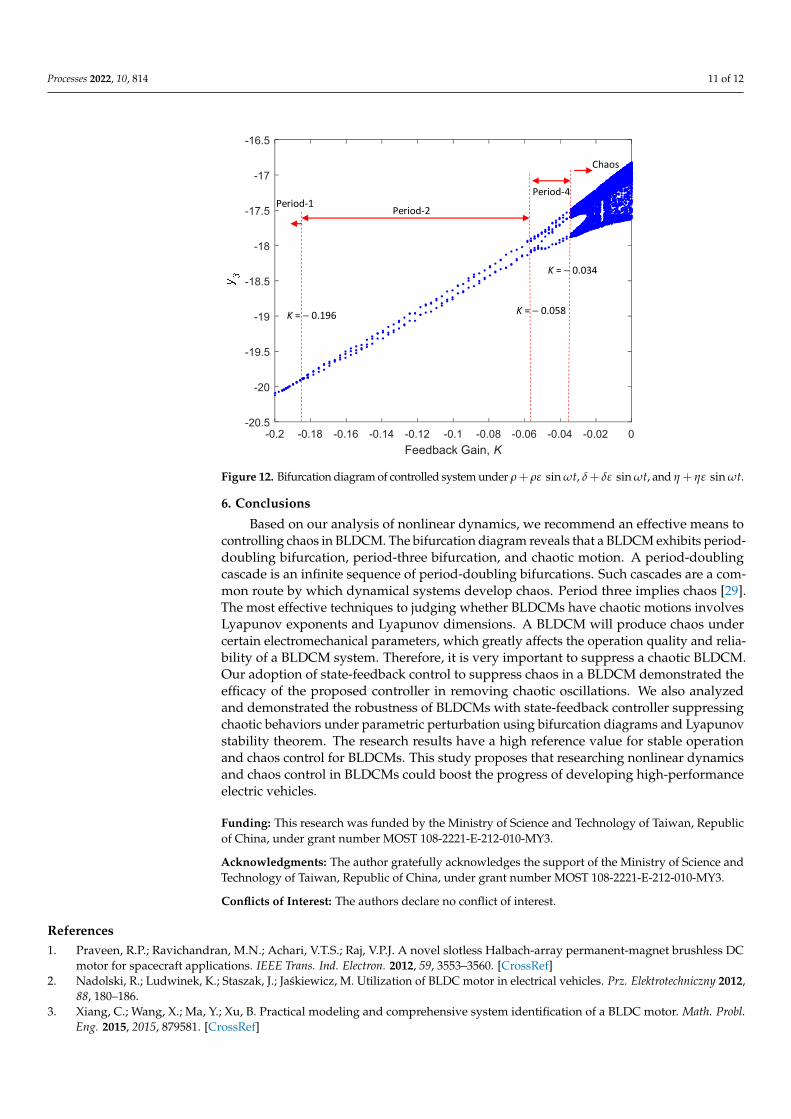
tions based on the following parameters: ε = 0.001 and ω = 125 rad/s. The detailed numeri-cal results are presented in Figure 11a–c. Figure 11a displays the results for e1 = v1 − y1,Figure 11b displays the results for e2 = v2 − y2, and Figure 11c displays the results fore3 = v3 − y3. Overall, the synchronization error converged to zero, thereby indicating thatthe two systems, which contained perturbated parameters, can synchronize the states ofthe drive system and the response system. This demonstrated that the suggested controlapproach is more robust to perturbated parameters in a BLDCM. Figure 12 presents a bifur-cation diagram demonstrating the efficacy of the recommended control approach describedin Equations (11)–(13) in suppressing chaotic behaviors under perturbed parameters.

Processes 2022, 10, x FOR PEER REVIEW 11 of 13

Figure 11. Dynamics of synchronization errors: (a) e1 = v1 − y1, (b) e2 = v2 − y2, and (c) e3 = v3 − y3.

Figure 12. Bifurcation diagram of controlled system under 𝜌 + 𝜌𝜀 sin𝜔𝑡 , 𝛿 + 𝛿𝜀 sin𝜔𝑡 , and 𝜂 +𝜂𝜀 sin𝜔𝑡.

6. Conclusions Based on our analysis of nonlinear dynamics, we recommend an effective means to

controlling chaos in BLDCM. The bifurcation diagram reveals that a BLDCM exhibits period-doubling bifurcation, period-three bifurcation, and chaotic motion. A period-doubling cascade is an infinite sequence of period-doubling bifurcations. Such cascades

0 5 10 15Time (sec)

0

0.005

0.01

0.015

0.02(a)

0 5 10 15Time (sec)

0

0.005

0.01(b)

0 5 10 15Time (sec)

0

0.01

0.02

0.03(c)

-0.2 -0.18 -0.16 -0.14 -0.12 -0.1 -0.08 -0.06 -0.04 -0.02 0Feedback Gain, K

-20.5

-20

-19.5

-19

-18.5

-18

-17.5

-17

-16.5

Period-1

K = − 0.19

Period-2

Period-4

K = − 0.055

K = − 0.032

Chaos

Figure 11. Dynamics of synchronization errors: (a) e1 = v1 − y1, (b) e2 = v2 − y2, and (c) e3 = v3 − y3.

Processes 2022, 10, 814 11 of 12

Processes 2022, 10, x FOR PEER REVIEW 11 of 13

Figure 11. Dynamics of synchronization errors: (a) e1 = v1 − y1, (b) e2 = v2 − y2, and (c) e3 = v3 − y3.

Figure 12. Bifurcation diagram of controlled system under 𝜌 + 𝜌𝜀 sin𝜔𝑡 , 𝛿 + 𝛿𝜀 sin𝜔𝑡 , and 𝜂 +𝜂𝜀 sin𝜔𝑡.

6. Conclusions Based on our analysis of nonlinear dynamics, we recommend an effective means to

controlling chaos in BLDCM. The bifurcation diagram reveals that a BLDCM exhibits period-doubling bifurcation, period-three bifurcation, and chaotic motion. A period-doubling cascade is an infinite sequence of period-doubling bifurcations. Such cascades

0 5 10 15Time (sec)

0

0.005

0.01

0.015

0.02(a)

0 5 10 15Time (sec)

0

0.005

0.01(b)

0 5 10 15Time (sec)

0

0.01

0.02

0.03(c)

-0.2 -0.18 -0.16 -0.14 -0.12 -0.1 -0.08 -0.06 -0.04 -0.02 0

Feedback Gain, K

-20.5

-20

-19.5

-19

-18.5

-18

-17.5

-17

-16.5

Period-1

K = − 0.196

Period-2

Period-4

K = − 0.058

K = − 0.034

Chaos

Figure 12. Bifurcation diagram of controlled system under ρ+ ρε sin ωt, δ+ δε sin ωt, and η + ηε sin ωt.

6. Conclusions

Based on our analysis of nonlinear dynamics, we recommend an effective means tocontrolling chaos in BLDCM. The bifurcation diagram reveals that a BLDCM exhibits period-doubling bifurcation, period-three bifurcation, and chaotic motion. A period-doublingcascade is an infinite sequence of period-doubling bifurcations. Such cascades are a com-mon route by which dynamical systems develop chaos. Period three implies chaos [29].The most effective techniques to judging whether BLDCMs have chaotic motions involvesLyapunov exponents and Lyapunov dimensions. A BLDCM will produce chaos undercertain electromechanical parameters, which greatly affects the operation quality and relia-bility of a BLDCM system. Therefore, it is very important to suppress a chaotic BLDCM.Our adoption of state-feedback control to suppress chaos in a BLDCM demonstrated theefficacy of the proposed controller in removing chaotic oscillations. We also analyzedand demonstrated the robustness of BLDCMs with state-feedback controller suppressingchaotic behaviors under parametric perturbation using bifurcation diagrams and Lyapunovstability theorem. The research results have a high reference value for stable operationand chaos control for BLDCMs. This study proposes that researching nonlinear dynamicsand chaos control in BLDCMs could boost the progress of developing high-performanceelectric vehicles.

Funding: This research was funded by the Ministry of Science and Technology of Taiwan, Republicof China, under grant number MOST 108-2221-E-212-010-MY3.

Acknowledgments: The author gratefully acknowledges the support of the Ministry of Science andTechnology of Taiwan, Republic of China, under grant number MOST 108-2221-E-212-010-MY3.

Conflicts of Interest: The authors declare no conflict of interest.

References1. Praveen, R.P.; Ravichandran, M.N.; Achari, V.T.S.; Raj, V.P.J. A novel slotless Halbach-array permanent-magnet brushless DC

motor for spacecraft applications. IEEE Trans. Ind. Electron. 2012, 59, 3553–3560. [CrossRef]2. Nadolski, R.; Ludwinek, K.; Staszak, J.; Jaskiewicz, M. Utilization of BLDC motor in electrical vehicles. Prz. Elektrotechniczny 2012,

88, 180–186.3. Xiang, C.; Wang, X.; Ma, Y.; Xu, B. Practical modeling and comprehensive system identification of a BLDC motor. Math. Probl.

Eng. 2015, 2015, 879581. [CrossRef]

Processes 2022, 10, 814 12 of 12

4. Huang, X.; Goodman, A.; Gerada, C.; Fang, Y. A single sided matrix converter drive for a brushless DC motor in aerospaceapplications. IEEE Trans. Ind. Electron. 2011, 59, 3542–3552. [CrossRef]

5. Srinivas, P. Design and FE Analysis of BLDC motor for electro-mechanical actuator. J. Electr. Syst. 2015, 11, 76–88.6. Jin, X.; Leng, J. Global exponential stabilization for brushless DC motors. Int. Core J. Eng. 2016, 2, 26–31.7. Gritli, H.; Belghith, S. Walking dynamics of the passive compass-gait model under OGY-based control: Emergence of bifurcations

and chaos. Commun. Nonlinear Sci. 2017, 47, 308–327. [CrossRef]8. Sajid, M. Chaotic behaviour and bifurcation in real dynamics of two-parameter family of functions including logarithmic map.

Abstr. Appl. Anal. 2020, 2020, 7917184. [CrossRef]9. Li, X.; Tan, Z.; Wang, X.; Liu, Y. Evolution of the discharge mode from chaos to an inverse period-doubling bifurcation in an

atmospheric-pressure He/N2 dielectric barrier discharge in increasing nitrogen content. IEEE Trans. Plasma Sci. 2022, 50, 619–634.[CrossRef]

10. Awal, N.M.; Epstein, I.R. Period-doubling route to mixed-mode chaos. Phys. Rev. E 2021, 104, 024211. [CrossRef]11. Chen, Z.; Xu, Y.; Ying, J. Analytical bifurcation tree of period-1 to period-4 motions in a 3-D brushless DC motor with voltage

disturbance. IEEE Access 2020, 8, 129613–129625. [CrossRef]12. Zhang, F.; Lin, D.; Xiao, M.; Li, H. Dynamical behaviors of the chaotic brushless DC motors model. Complexity 2016, 21, 79–85.

[CrossRef]13. Zhou, Y.; Zhao, K.; Liu, D. Chaotic dynamic analysis of brushless DC motor. J. Math. Inform. 2016, 5, 39–43.14. Wolf, A.; Swift, J.B.; Swinney, H.L.; Vastano, J.A. Determining Lyapunov exponent from a time series. Phys. D 1985, 16, 285–317.

[CrossRef]15. Ge, Z.M.; Chang, C.M.; Chen, Y.S. Anti-control of chaos of single time scale brushless dc motors and chaos synchronization of

different order systems. Chaos Soliton Fract. 2006, 27, 1298–1315. [CrossRef]16. Roy, P.; Ray, S.; Bhattacharya, S. Control of chaos in brushless DC motor design of adaptive controller following back-stepping

method. In Proceedings of the 2014 International Conference on Control, Instrumentation, Energy and Communication (CIEC),Calcutta, India, 31 January–2 February 2014.

17. Kose, E.; Muhurcu, A. The control of brushless DC motor for electric vehicle by using chaotic synchronization method. Stud.Inform. Control 2018, 27, 403–412. [CrossRef]

18. Cai, C.; Xu, Z.; Xu, W. Converting chaos into periodic motion by state feedback control. Automatica 2002, 38, 1927–1933. [CrossRef]19. Chang, S.C.; Lin, H.P. Chaos attitude motion and chaos control in an automotive wiper system. Int. J. Solids Struct. 2004,

41, 3491–3504. [CrossRef]20. Chang, S.C. Adoption of state feedback to control dynamics of vehicle with steer-by-wire system. Proc. Inst. Mech. Eng. D J.

Automob. Eng. 2007, 221, 1–12. [CrossRef]21. Rafikov, M.; Balthazar, J.M. On an optimal control design for Rossler system. Phys. Lett. A 2004, 333, 241–245. [CrossRef]22. Rafikov, M.; Balthazar, J.M. On control and synchronization in chaotic and hyperchaotic systems via linear feedback control.

Commun. Nonlinear Sci. Numer. Simul. 2008, 13, 1246–1255. [CrossRef]23. Rafikov, M.; Balthazar, J.M.; Tusset, A.M. An optimal linear control design for nonlinear systems. J. Braz. Soc. Mech. Sci. Eng. 2008,

30, 279–284. [CrossRef]24. Hemati, N.; Leu, M.C. A complete model characterization of brushless DC motors. IEEE Trans. Ind. Appl. 1992, 28, 172–180.

[CrossRef]25. Hemati, N. Strange attractors in brushless DC motors. IEEE Trans. Circuits Syst. I Fundam. Theory Appl. 1994, 41, 40–45. [CrossRef]26. Hemati, N. Dynamic analysis of brushless motors based on compact representations of the equations of motion. In Proceedings

of the Conference Record of the 1993 IEEE Industry Applications Conference Twenty-Eighth IAS Annual Meeting, Toronto, ON,Canada, 2–8 October 1993.

27. IMSL, Inc. User’s Manual−IMSL; MATH/LIBRARY: Houston, TX, USA, 1989.28. Guckenheimer, J.; Holmes, P. Nonlinear Oscillations, Dynamical Systems, and Bifurcations of Vector Fields; Springer: Berlin/Heidelberg,

Germany; Dordrecht, The Netherlands; New York, NY, USA, 2013; Volume 42.29. Li, T.Y.; Yorke, J.A. Period three implies chaos. Am. Math. Mon. 1975, 82, 985–992. [CrossRef]30. Kaplan, J.L.; Yorke, J.A. Chaotic Behavior of Multidimensional Difference Equations, Lecture Notes in Mathematics; Springer: New York,

NY, USA, 1979.31. Khalil, H.K. Nonlinear Systems, 3rd ed.; Prentice-Hall: Hoboken, NJ, USA, 2002.