ARTICLE IN PRESS

JOURNAL OFSOUND ANDVIBRATION

0022-460X/$ - s

doi:10.1016/j.js

�CorrespondE-mail addr

Journal of Sound and Vibration 294 (2006) 585–595

www.elsevier.com/locate/jsvi

Short Communication

Chaos and transient chaos in an experimentalnonlinear pendulum

Aline Souza de Paula, Marcelo Amorim Savi�, Francisco Heitor Iunes Pereira-Pinto

COPPE - Department of Mechanical Engineering, Universidade Federal do Rio de Janeiro, P.O. Box 68.503,

21.941.972 Rio de Janeiro, RJ, Brazil

Received 15 April 2005; received in revised form 21 October 2005; accepted 11 November 2005

Available online 18 January 2006

Abstract

Pendulum is a mechanical device that instigates either technological or scientific studies, being associated with the

measure of time, stabilization devices as well as ballistic applications. Nonlinear characteristic of the pendulum attracts a

lot of attention being used to describe different phenomena related to oscillations, bifurcation and chaos. The main

purpose of this contribution is the analysis of chaos in an experimental nonlinear pendulum. The pendulum consists of a

disc with a lumped mass that is connected to a rotary motion sensor. This assembly is driven by a string–spring device that

is attached to an electric motor and also provides torsional stiffness to the system. A magnetic device provides an

adjustable dissipation of energy. This experimental apparatus is modeled and numerical simulations are carried out. Free

and forced vibrations are analyzed showing that numerical results are in close agreement with those obtained from

experimental data. This analysis shows that the experimental pendulum has a rich response, presenting periodic response,

chaos and transient chaos.

r 2006 Elsevier Ltd. All rights reserved.

1. Introduction

Chaotic behavior of physical systems has been extensively analyzed from the early sixties when E. Lorenzdevelops studies on the unpredictability of meteorological phenomena. Nowadays, different fields of scienceshave special interest in this kind of phenomenon as for example engineering, medicine, ecology, biology andeconomy.

Mechanical sciences are also included in these areas presenting different situations where chaos appears.Nonlinear pendulum is a mechanical device that attracts a lot of attention being used to describe differentphenomena related to oscillations, bifurcation and chaos. Actually, pendulum instigates either technologicalor scientific studies, being associated with the measure of time, stabilization devices as well as ballisticapplications. As a matter of fact, the interest in the study of pendulum motion is old. Galileo (1564–1642)dedicates many efforts to the pendulum analysis where its use should be pointed out for the measure of time.Foucault (1819–1868) presents the first evidence that earth rotates on its axis using a pendulum. It was

ee front matter r 2006 Elsevier Ltd. All rights reserved.

v.2005.11.015

ing author.

ess: savi@ufrj.br (M.A. Savi).

ARTICLE IN PRESSA.S. de Paula et al. / Journal of Sound and Vibration 294 (2006) 585–595586

constructed by suspending a pendulum on a long wire from the dome of the Pantheon in Paris. During thehistory, many studies are carried out analyzing the pendulum dynamics and, certainly, pendulum becomes oneof the paradigms in the study of physics and natural phenomena [1].

Regarding the experimental point of view, it is possible to say that experimental findings do not precedetheoretical development of nonlinear sciences [2]. However, by observing the words of Poincare, a pioneer onthe nonlinear dynamics and chaos, ‘‘experiment is the sole source of truth’’, it is possible to argue thatexperimental approach tends to grow in nonlinear sciences evaluating different details of the so-called chaostheory. By examining the literature related to experimental analysis of nonlinear pendulum, differentmechanical and electrical devices are proposed in order to describe the main characteristics of the pendulummotion [3–6]. Nevertheless, this experimental analysis is complex, especially when it deals with mechanicalsystems.

The main purpose of this contribution is the analysis of chaos in an experimental nonlinear pendulum. Theexperimental apparatus was previously presented in Refs. [3,7]. This pendulum has both torsional stiffness anddamping. Franca and Savi [8] treat the dynamics of this pendulum in the framework of time-series analysis.Pinto and Savi [9] investigate the signal prediction while Pereira-Pinto et al. [10,11] discuss its chaos control.Here, this problem is revisited exploiting details of its nonlinear dynamics. Essentially, experimental apparatusis modeled and numerical simulations are carried out allowing a comparison with experimental data. Resultsshow that they are in close agreement presenting a rich response which includes chaos and transient chaos.

2. Experimental apparatus and mathematical model

Consider the experimental nonlinear pendulum which is shown in Fig. 1. The right-hand side presents theexperimental apparatus while the left-hand side shows its schematic picture. Basically, the pendulum consistsof an aluminum disc (1) with a lumped mass (2) that is connected to a rotary motion sensor (4), PASCO CI-6538, which has a precision of 70.251, maximum velocity of 30 revolutions/s and maximum samplingfrequency of 1000Hz. This assembly is driven by a string-spring device (6) that is attached to an electric motor(7) (PASCO ME-8750 with 0–12 eV, 0–0.3A) and also provides torsional stiffness to the system. A magneticdevice (3) provides an adjustable dissipation of energy.

Fig. 1. Nonlinear pendulum: (a) physical model—(1) metallic disc; (2) lumped mass; (3) magnetic damping device; (4) rotary motion

sensor (PASCO CI-6538); (5) anchor mass; (6) string–spring device; (7) electric motor (PASCO ME-8750). (b) Parameters and forces on

the metallic disc. (c) Parameters from driving device. (d) Experimental apparatus.

ARTICLE IN PRESSA.S. de Paula et al. / Journal of Sound and Vibration 294 (2006) 585–595 587

2.1. Mathematical model

In order to obtain the equations of motion of the experimental nonlinear pendulum it is assumed thatsystem dissipation may be expressed by a combination of a linear viscous dissipation together with dryfriction. Therefore, denoting the angular position as, f, the following equation is obtained:

€fþzI_fþ

kd2

2Ifþ

m sgn ð _fÞI

þmgD sin ðfÞ

2I¼

kd

2I

ffiffiffiffiffiffiffiffiffiffiffiffiffiffiffiffiffiffiffiffiffiffiffiffiffiffiffiffiffiffiffiffiffiffiffiffiffiffiffiffiffiffiffiffiffia2 þ b2

� 2ab cos ðotÞ

q� ða� bÞ

� �, (1)

where o is the forcing frequency related to the motor rotation, a defines the position of the guide of the stringwith respect to the motor, b is the length of the excitation crank of the motor, D is the diameter of the metallicdisc and d is the diameter of the driving pulley, m is the lumped mass, z represents the linear viscous dampingcoefficient, while m is the dry friction coefficient; g is the gravity acceleration, I is the inertia of the disk-lumpedmass and k is the string stiffness. Moreover, sgn(x) is the sign of the variable x.

In order to model the dry friction in a continuous form, the following relation is used [12]:

m sgn ð _fÞ ¼2

pm arctan ðq _fÞ, (2)

where q assumes a great value, for example, q ¼ 106. The equation of motion may be written in terms ofa first-order differential equations system with the form, _x ¼ f ðx; tÞ; x 2 R2. It should be pointed out thatthe system dynamics depends on the position of the motor rotating crank. The angular position ismeasured from the vertical position of the crank, being positive when rotating in a counter-clockwisedirection. Therefore, it is interesting to identify the position of the rotating crank, calling this as motorphase, y.

2.2. Parameters identification

Geometrical properties of the pendulum may be easily measured, and the following values are obtained:a ¼ 1:6� 10�1 m; b ¼ 6:0� 10�2 m; d ¼ 4:8� 10�2 m; D ¼ 9:5� 10�2 m. The lumped mass can be measuredwith a weight scale, and it is identified as m ¼ 1:47� 10�2 kg.

After that, it is possible to identify inertia of this system by evaluating the dynamics of the disc subjectedto a known torque. Basically, the experimental procedure considers a mass attached to a string that isrolled up in a pulley, attached to a rotary sensor. Suddenly, the mass is released from the equilibrium,subjected to the action of gravity. Assuming a mass of 1.47� 10�2 kg and a pulley with radius 1.45� 10�2m, itis possible to estimate the inertia as Idisc ¼ mgr= €f. Since the value of the acceleration measured from therotary sensor is €f ¼ 24:6 rad=s2 and g ¼ 9:81m=s2, one concludes that Idisc ¼ 1:407� 10�4 kgm2. Now, it ispossible to estimate the inertia of the disc-lumped mass system considering that I ¼ mD2=4þ Idisc ¼

1:738� 10�4 kgm2.The spring stiffness is evaluated as the slope of a force–displacement curve, plotted with the aid of two

sensors: the rotary sensor shown in Fig. 1 and a force sensor (PS-2104), which has a range of 750N, with 1%of accuracy and resolution of 0.03N. This procedure identifies springs with k ¼ 2:47N=m.

Since the system dissipation characteristics are due to linear viscous damping and also due to dry friction,different procedures must be employed in order to estimate dissipation parameters. Basically, the free responseof the pendulum is analyzed, assuming ðf; _fÞ ¼ ðp=2; 0Þ as initial condition and phase angle y ¼ 0. In general,it is observed that for the beginning of the motion, when velocities are greater, linear viscous damping ispreponderant. As time increases, and the velocity decreases, dry friction becomes more important. Therefore,dissipation parameters are evaluated considering logarithmic decrement procedure for the first part of themovement, while the second part assumes that the differences between two consecutive peaks have a lineardecrement. Measuring the decay in the first part, one obtains x ¼ 0:017 and therefore, z ¼ 2xIo0 ¼

2:368� 10�5 kgm2=s. For the second part of the oscillation, it is measured the difference between twoconsecutive peaks Dx ¼ 0:0525 and therefore m ¼ ðk0=4Þ Dx ¼ 1:272� 10�4 Nm. Here k0 is related to thelinearized stiffness of the system, k0 ¼ ðkd2

þmgDÞ=2.

ARTICLE IN PRESSA.S. de Paula et al. / Journal of Sound and Vibration 294 (2006) 585–595588

3. Free response

In order to start the analysis of the nonlinear experimental pendulum dynamics, free response is focused on.The classical fourth-order Runge–Kutta method is employed for all numerical simulations. The point x is anequilibrium point of the system _x ¼ f ðxÞ, if f ðxÞ ¼ 0. Moreover, the system dynamics in the neighborhood of apoint may be analyzed by the eigenvalues of the Jacobian matrix, A ¼ Df . Therefore, from equations ofmotion it is possible to conclude that the number and also the characteristics of the equilibrium points of theexperimental pendulum depends on the motor phase, y. Fig. 2 presents a picture related to these equilibriumpoints, obtained by analytical and experimental approaches. It shows that the system has only one stable pointfor small values of y, a stable spiral, and the same behavior for higher values (0oyo2:17 and 4:11oyo2p).However, for intermediate values ð2:17pyp4:11Þ, there are three equilibrium points. For those, two are stable(stable spiral) and the other is unstable, a saddle node.

These results may be confirmed by considering the pendulum free response for different initial conditionsand also motor phase. Fig. 3 presents some of these responses, showing the stable equilibrium pointsdepending on the motor phase. Basically, two different motor phases are considered: y ¼ p and p=2. Note thatfor y ¼ p, there are two stable spiral responses and, between these points, there is an unstable point (notshown). On the other hand, for y ¼ p=2, there is only a single stable spiral equilibrium point.

Fig. 2. Equilibrium points map. — stable spiral, - - - saddle, experimental points.

Fig. 3. Free responses for different initial conditions and different value of y, — experimental, - - - numerical. (a) y ¼ p; (b) y ¼ p=2.

ARTICLE IN PRESSA.S. de Paula et al. / Journal of Sound and Vibration 294 (2006) 585–595 589

4. Forced response

Forced response of the experimental pendulum is much more complex. In order to perform a global analysisof different kinds of response, bifurcation diagram is constructed, sampling angular position against the slowquasi-static variation of the forcing frequency parameter. Basically, this diagram is constructed by assumingsimilar initial condition for each parameter value, neglecting the first 2000 periods. This procedure is carriedout numerically and confirmed with experiments in some frequencies (Fig. 4). This diagram allows one toobserve regions related to periodic and chaotic motion.

Now, different kinds of response are considered, comparing numerical results with those obtainedexperimentally. Fig. 5 shows periodic responses for different forcing frequency: o ¼ 3:59 rad=s ando ¼ 5:1 rad=s. It should be pointed out the close agreement between numerical and experimental results.By changing the forcing frequency for o ¼ 5:61 rad=s, a value inside a chaotic region of the bifurcationdiagram, chaos appears. Fig. 6 presents state space for both numerical and experimental results, showingagain, a close agreement. Lyapunov exponents assure the conclusion about chaotic response. Employing thealgorithm due to Wolf et al. [13], the spectrum is l ¼ ðþ0:4483;�0:5732Þ.

Fig. 4. Bifurcation diagram: experimental, numerical.

Fig. 5. Periodic forced response for different forcing frequency, — experimental. - - - numerical: (a) o ¼ 3:59 rad=s; (b) o ¼ 5:1 rad=s.

ARTICLE IN PRESS

Fig. 6. Chaotic response for o ¼ 5:61 rad=s: (a) experimental; (b) numerical.

Fig. 7. Strange attractors for o ¼ 5:61 rad=s: (a, c) experimental; (b, d) numerical.

A.S. de Paula et al. / Journal of Sound and Vibration 294 (2006) 585–595590

Poincare section is a procedure which eliminates time variable by sampling state variables at a rate equal tothe forcing period. Basically, it shows the intersections of the orbit with a plane, and chaotic attractor isusually strange in the sense that has a non-integer dimension [14]. Fig. 7 presents both experimental andnumerical strange attractors, considering different positions of the section, separated by p. Experimentalconstruction is done considering an analysis of the time series, sampling its values when it crosses a definedsurface. The definition of the surface is done considering a signal related to the motor position which is

ARTICLE IN PRESSA.S. de Paula et al. / Journal of Sound and Vibration 294 (2006) 585–595 591

obtained with the aid of a rotary sensor, similar to the one used to measure the pendulum position. A goodagreement between numerical and experimental strange attractors is noticeable.

A geometrical form to understand chaos is related to a transformation known as Smale horseshoe.Basically, it establishes a sequence of contraction–expansion–folding which causes the existence of an infinitenumber of unstable periodic orbits (UPOs) embedded in a strange attractor [15,16]. Here, the close returnmethod [17] is employed in order to evaluate the UPOs embedded in the experimental strange attractordiscussed in Fig. 7. Fig. 8 shows some orbits identified in the attractor employing the cited close returnmethod. On the other hand, Fig. 9 presents some of these orbits in the phase space.

The term transient chaos is used to describe a chaotic-like response, which becomes periodic after somecycles. Therefore, under this condition, after a finite time, the orbit leaves the chaotic region, establishing aperiodic or quasi-periodic motion [18]. Grebogi et al. [19] defines crises phenomenon as a collision between achaotic attractor and a coexisting unstable fixed point or periodic orbit. The cited reference also argues thatcrises appear to be the cause of most sudden changes in chaotic dynamics. Therefore, transient chaos andcrises are related. The nonlinear pendulum dynamics presents an interesting behavior related to this kind ofbehavior, and in order to analyze it, bifurcation diagram is revisited, enlarging a region related to transientchaos. Now, three different procedures are employed to construct two bifurcation diagrams. The first oneconsiders similar initial conditions for each parameter value, neglecting the first 4000 periods (Fig. 10a). Thesecond procedure neglects the first 150 periods considering the same initial conditions, which allows observing

Fig. 8. Unstable periodic orbits embedded in strange attractor. ’ UPO period 3, K UPO period 5, m UPO period 5, ~ UPO period 7.

Fig. 9. Unstable periodic orbits: (a) period-3; (b) period-5; (c) period-7.

ARTICLE IN PRESS

Fig. 10. Bifurcation diagram plotted by different procedures: (a) first and second procedures; (b) third and second procedures.

Fig. 11. Transient chaos: (a) experimental, (b) numerical.

A.S. de Paula et al. / Journal of Sound and Vibration 294 (2006) 585–595592

part of the transient. The third procedure considers stabilized values of state variables as an initial conditionfor the next parameter value, neglecting 150 periods (Fig. 10b). The second procedure is shown in bothdiagrams allowing the transient chaos visualization, in background. Note that the third procedure is not ableto capture neither the coexistence of different attractors nor the transient chaos.

Transient chaos is related to an irregular motion that tends to stabilize in a periodic motion after a longtransient response. Fig. 11 presents both experimental and numerical results of this response foro ¼ 6:23 rad=s. The analysis of Lyapunov exponents shows that the response presents a positive value thattends to become negative after the stabilization. During transient chaos, the spectrum is l ¼ ðþ0:5;�0:6Þ.However, in steady state, the spectrum is l ¼ ð�0:0323;�0:0914Þ.

The transient chaos is also related to a fractal-like structure during the transient response, tending to beeliminated in the steady state. This is usually denominated chaotic saddle, being geometrically related to thestrange attractor, but with repulsive characteristics. Fig. 12a shows this chaotic saddle and also the period-1steady-state response. Fig. 12b, on the other hand, shows the period-1 steady-state orbit obtained either bynumerical or by experimental approaches.

Another characteristic of the transient chaos is the sensitive dependence to initial conditions, which could bepointed out by some simulations. Fig. 13 presents simulations for o ¼ 6:23 rad=s and different initialconditions. At first, two different, very close, initial conditions are considered (Fig. 13a and b). Theseresponses are related to the same steady-state orbit, which, presents a different transient response. Byconsidering proper initial conditions, transient response can be eliminated. Fig. 13c shows a situation where

ARTICLE IN PRESS

Fig. 13. Transient responses for different initial conditions: (a) ðf; _fÞ ¼ ð0:00293; 0:1421Þ; (b) ðf; _fÞ ¼ ð0:00292; 0:14205Þ; (c)

ðf; _fÞ ¼ ð2:8;�2:2Þ.

Fig. 12. (a) Chaotic saddle and the steady-state period-1 response; (b) period-1 steady state. — Experimental, - - - numerical.

A.S. de Paula et al. / Journal of Sound and Vibration 294 (2006) 585–595 593

the steady-state orbit is achieved in the beginning of the motion. Similar situations could be seen in bifurcationdiagrams. Therefore, it is possible to conclude that the existence of transient chaos depends on initialconditions.

By observing bifurcation diagram, there is a region related to the coexistence of stable attractors. Note thatfor oo6:235 rad=s or o46:290 rad=s there is only a period-1 attractor. Other regions have different coexistingattractors. For example, when o ¼ 6:240 rad=s, there are a period-4 and a period-1 coexisting attractors. Asmall change for o ¼ 6:245 rad=s may cause the appearance of three attractors: period-4, period-8 and period-1. By changing o ¼ 6:250 rad=s, period-4 orbit disappears, remaining only period-8 and period-1 orbits. Wheno ¼ 6:250 rad=s, period-4 orbit appears instead of period-8 orbit.

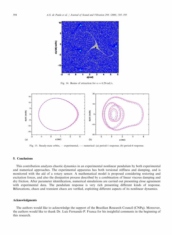
The coexistence of attractors may be assured constructing basins of attraction. For o ¼ 6:23 rad=s, basinsof attraction show just one steady-state orbit. However, by considering a different frequency parameter(o ¼ 6:28 rad=s, for example), there are two coexisting attractors, as can be identified in bifurcation diagrams.The first one is a period-1 while the second corresponds to a period-4 response. Basins of attraction alsoillustrate this coexistence (Fig. 14). The dark color is associated with a period-4 response while the gray coloris related to a period-1 response. For initial conditions in the neighborhood of the periodic attractors, period-1or period-4, there is no transient chaos. On the other hand, the basins of attraction for regions far from theneighborhood of these points are mixed, being related to a transient chaos before the stabilization. Althoughthese are not well-defined regions of initial conditions that lead to the periodic attractors in the mixed portion,roughly 75% of these initial conditions drive the system trajectory to the period-4 orbit. Fig. 15 shows bothsteady-state orbits obtained by numerical and experimental approaches.

ARTICLE IN PRESS

Fig. 15. Steady-state orbits, — experimental, - - - numerical: (a) period-1 response; (b) period-4 response.

Fig. 14. Basins of attraction for o ¼ 6:28 rad=s.

A.S. de Paula et al. / Journal of Sound and Vibration 294 (2006) 585–595594

5. Conclusions

This contribution analyzes chaotic dynamics in an experimental nonlinear pendulum by both experimentaland numerical approaches. The experimental apparatus has both torsional stiffness and damping, and ismonitored with the aid of a rotary sensor. A mathematical model is proposed considering restoring andexcitation forces, and also the dissipation process described by a combination of linear viscous damping anddry friction. After parameter identification, numerical simulations are carried out presenting close agreementwith experimental data. The pendulum response is very rich presenting different kinds of response.Bifurcations, chaos and transient chaos are verified, exploiting different aspects of its nonlinear dynamics.

Acknowledgments

The authors would like to acknowledge the support of the Brazilian Research Council (CNPq). Moreover,the authors would like to thank Dr. Luiz Fernando P. Franca for his insightful comments in the beginning ofthis research.

ARTICLE IN PRESSA.S. de Paula et al. / Journal of Sound and Vibration 294 (2006) 585–595 595

References

[1] J.L. Trueba, J.P. Baltanas, M.A.F. Sanjuan, A generalized perturbed pendulum, Chaos, Solitons and Fractals 15 (2003) 911–924.

[2] L. Werner, T. Kurz, U. Parlitz, Experimental nonlinear physics, Journal of the Franklin Institute 334B (5/6) (1997) 865–907.

[3] J.A. Blackburn, G.L. Baker, A comparison of commercial chaotic pendulums, American Journal of Physics 66 (9) (1998) 821–829.

[4] D. D’Humieres, M.R. Beasley, B.A. Huberman, A. Libehaber, Chaotic states and routes to chaos in the forced pendulum, Physical

Review A 26 (6) (1982) 3483–3496.

[5] T. Shinbrot, C. Grebogi, J. Wisdom, J.A. Yorke, Chaos in a double pendulum, American Journal of Physics 60 (6) (1992) 491–499.

[6] Q. Zhu, M. Ishitobi, Experimental study of chaos in a driven triple pendulum, Journal of Sound and Vibration 227 (1) (1999) 230–238.

[7] R. DeSerio, Chaotic pendulum: the complete attractor, American Journal of Physics 71 (3) (2003) 250–256.

[8] L.F.P. Franca, M.A. Savi, Distinguishing periodic and chaotic time series obtained from an experimental nonlinear pendulum,

Nonlinear Dynamics 26 (3) (2001) 253–271.

[9] E.G.F. Pinto, M.A. Savi, Nonlinear prediction of time series obtained from an experimental pendulum, Current Topics in Acoustical

Research—Research Trends 3 (2003) 151–162.

[10] F.H.I. Pereira-Pinto, A.M. Ferreira, M.A. Savi, Chaos control in a nonlinear pendulum using a semi-continuous method, Chaos,

Solitons and Fractals 22 (3) (2004) 653–668.

[11] F.H.I. Pereira-Pinto, A.M. Ferreira, M.A. Savi, State space reconstruction using extended state observers to control chaos in a

nonlinear pendulum, International Journal of Bifurcation and Chaos 15 (2005), in press.

[12] R.I. Leine, Bifurcations in Discontinuous Mechanical Systems of Filippov-type, Ph.D. Thesis, Technische Universiteit Eindhoven,

2000.

[13] A. Wolf, J.B. Swift, H.L. Swinney, J.A. Vastano, Determining Lyapunov exponents from a time series, Physica D 16 (1985) 285–317.

[14] C. Grebogi, E. Ott, S. Pelikan, J.A. Yorke, Strange attractors that are not chaotic, Physica 13D (1–2) (1984) 261–268.

[15] J. Guckenheimer, P. Holmes, Nonlinear Oscillations, Dynamical Systems, and Bifurcations of Vector Fields, Springer, Berlin, 1983.

[16] S. Wiggins, Introduction to Applied Nonlinear Dynamical Systems and Chaos, Springer, Berlin, 1990.

[17] D. Auerbach, P. Cvitanovic, J.-P. Eckmann, G. Gunaratne, I. Procaccia, Exploring chaotic motion through periodic orbits, Physical

Review Letters 58 (23) (1987) 2387–2389.

[18] F.C. Moon, Chaotic and Fractal Dynamics, Wiley, New York, 1992.

[19] C. Grebogi, E. Ott, J.A. Yorke, Crises, sudden changes in chaotic attractors, and transient chaos, Physica 7D (1983) 181–200.