June 19, 2012 18:5 WSPC/S0218-1274 1250111

International Journal of Bifurcation and Chaos, Vol. 22, No. 5 (2012) 1250111 (14 pages)c© World Scientific Publishing CompanyDOI: 10.1142/S0218127412501118

BIFURCATION CONTROLOF A PARAMETRIC PENDULUM

ALINE S. DE PAULADepartment of Mechanical Engineering, Universidade de Brasılia,

70.910.900, Brasılia, DF, Brazilalinedepaula@unb.br

MARCELO A. SAVICOPPE/Department of Mechanical Engineering,

Universidade Federal do Rio de Janeiro,21.941.972, Rio de Janeiro, RJ, P. O. Box 68.503, Brazil

savi@mecanica.ufrj.br

MARIAN WIERCIGROCH∗ and EKATERINA PAVLOVSKAIA†Centre for Applied Dynamics Research, School of Engineering,

University of Aberdeen, AB24 3UE, Aberdeen, UK∗m.wiercigroch@abdn.ac.uk†e.pavlovskaia@abdn.ac.uk

Received January 26, 2011; Revised March 31, 2011

In this paper, we apply chaos control methods to modify bifurcations in a parametric pendulum-shaker system. Specifically, the extended time-delayed feedback control method is employed tomaintain stable rotational solutions of the system avoiding period doubling bifurcation andbifurcation to chaos. First, the classical chaos control is realized, where some unstable peri-odic orbits embedded in chaotic attractor are stabilized. Then period doubling bifurcation isprevented in order to extend the frequency range where a period-1 rotating orbit is observed.Finally, bifurcation to chaos is avoided and a stable rotating solution is obtained. In all cases,the continuous method is used for successive control. The bifurcation control method proposedhere allows the system to maintain the desired rotational solutions over an extended range ofexcitation frequency and amplitude.

Keywords : Nonlinear dynamics; chaos; control; parametric pendulum.

1. Introduction

The dynamics of a parametrically excited pendulumhas been extensively investigated in the literature.It has been found that this system can generatevarious types of motion, from simple periodic oscil-lations to complex chaos. While the majority ofthe authors analyzed oscillatory motion, i.e. [Xuet al., 2005; Bishop et al., 2005; Clifford & Bishop,1994, 1996], the rotational solutions received less

attention in the past. Nevertheless, a number ofpapers deal with the rotational solutions of thependulum under parametric excitation, and theyare briefly summarized as follows. Koch and Leven[1985] detected bifurcations of the system whereharmonic and subharmonic rotating solutions areborn by applying the Melnikovs method. Cliffordand Bishop [1995], Garira and Bishop [2003]numerically identified types of rotating solutions

†Author for correspondence

1250111-1

June 19, 2012 18:5 WSPC/S0218-1274 1250111

A. S. De Paula et al.

and classified them. Szemplinska-Stupnicka et al.[2000], Szemplinska-Stupnicka and Tyrkiel [2002]numerically investigated global bifurcations andvarious other aspects of the pendulum dynam-ics including fractal basin boundaries and coexis-tence of rotating solutions. Xu et al. [2005] andmost recently Horton et al. [2011] have performedextensive numerical simulations concerning differ-ent kinds of rotations, together with oscillations andchaos. Capecchi and Bishop [1990], Xu and Wier-cigroch [2007] and Lenci et al. [2008] investigatedrotating solutions analytically.

Although these rotating solutions are found andstudied by different authors, it should be pointedout that they only exist over limited parametersrange and there are a lot of bifurcations of the sys-tem that destabilize this kind of motion. In thisregard, the bifurcation control can be useful inmaintaining the rotational solutions.

The idea of controlling bifurcation is basedon modifying the considered nonlinear system toachieve some desirable dynamical behavior by con-structing and applying a controller [Abed & Fu,1986, 1987; Wen et al., 2006; Chen et al., 2000,2003; Xiao & Cao, 2009]. Concerning the rotatingsolutions, the idea is to maintain stability of thismotion avoiding either period doubling bifurcationor bifurcation to chaos.

Chaos control exploits the richness of chaoticbehavior and may be understood as the use ofperturbations for the stabilization of an UnstablePeriodic Orbit (UPO) embedded in a chaoticattractor. Chaos control methods are generallydivided into discrete and continuous techniques.The continuous methods are exemplified by the so-called delayed feedback control, proposed by Pyra-gas [1992], which states that chaotic systems canbe stabilized by a feedback perturbation propor-tional to the difference between the present anda delayed state of the system. Numerous researchefforts have been dedicated since then to overcomesome limitations of the original technique. Pyra-gas [2006] presents a review concerning improve-ments and applications of time-delayed feedbackmethods.

In this work, continuous chaos control methodsare employed in order to maintain rotating solu-tions of the pendulum system by stabilizing unsta-ble periodic orbits of the system. Hence, the maingoal here is to avoid bifurcations that destabilizethe rotating motion.

The interest in these rotational solutions ismotivated by an idea of energy harvesting from thesea waves using a pendulum system. The conceptconsists in converting the base oscillations of thestructure into a rotational motion of the pendulummass as proposed by Wiercigroch [2003]. In suchcase, the oscillations of the structure are causedby the sea waves, whereas the pendulum rotationalmotion provides a driving torque for an electricalgenerator [Xu, 2005; Horton, 2009; Horton & Wier-cigroch, 2008]. In order to explore potentials of thisconcept, the dynamics of the pendulum system hasto be carefully considered and the means of main-taining the periodic rotational solutions have to bedeveloped.

The paper is organized as follows. In thenext section continuous chaos control methods areintroduced. Then the studied system is presentedin Sec. 3, and in Sec. 4, chaos control methodsare employed aiming to stabilize unstable periodicorbits embedded into the chaotic attractors, orextend the stability range of the existing periodicorbits by avoiding period doubling bifurcations andbifurcations to chaos.

2. Chaos Control Methods

Chaos control may be understood as the use of smallperturbations in order to stabilize unstable periodicorbits. Typically, it is a two-stage procedure includ-ing learning stage and control stage. Since unsta-ble periodic orbits are part of the system dynamics,the stabilization of these orbits is associated withlow energy consumption. Therefore, this procedureis useful for different applications being of specialinterest in order to design flexible systems.

Chaos control methods can be split into discreteand continuous methods. Continuous methods arebased on continuous-time perturbations to performstabilization. This approach was first proposed byPyragas [1992] and deals with a dynamical systemmodeled by a set of ordinary nonlinear differentialequations as follows:

x(t) = Q(x, t) + B(t), (1)

where t is time, x(t) ∈ n is the state variablevector, Q(x, t) ∈ n defines the system dynam-ics, while B(t) ∈ n is associated with the controlaction.

Socolar et al. [1994] proposed a control lawnamed as the Extended Time-Delayed Feedbackcontrol (ETDF) considering the information of

1250111-2

June 19, 2012 18:5 WSPC/S0218-1274 1250111

Bifurcation Control of a Parametric Pendulum

time-delayed states of the system represented by thefollowing equations:

B(t) = K[(1 − R)Sτ − x],

Sτ =Nτ∑

m=1

Rm−1xmτ ,(2)

where K ∈ n×n is the feedback gain matrix,0 ≤ R < 1 is a control gain, Sτ = S(t − τ) andxmτ = x(t − mτ) are related to delayed states ofthe system and τ is the time delay. In general, Nτ isinfinity but it can be more precisely defined depend-ing on the dynamical system. The UPO stabiliza-tion can be achieved by an appropriate choice of Kand R. Note that for any gain defined by K andR, the perturbation of Eq. (2) vanishes when thesystem is on the UPO since x(t − mτ) = x(t) forall m if τ = Ti, where = Ti is the periodicity of theith UPO. It should be pointed out here that whenR = 0, the ETDF turns into the original Time-Delayed Feedback control method (TDF) proposedby Pyragas [1992].

The controlled dynamical system consists of aset of Delay Differential Equations (DDEs). Thesolution of this system is done by establishing an ini-tial function x0 = x0(t) over the interval (−Nττ, 0).This function can be estimated by a Taylor seriesexpansion as proposed by Cunningham [1954]:

xmτ = x − mτ x. (3)

Under this assumption, the following system isobtained:

x = Q(x, t) + K[(1 − R)Sτ − x],

where

Sτ =

Nτ∑m=1

Rm−1[x− mτ x], for (t − Nττ) < 0,

Nτ∑m=1

Rm−1xmτ , for (t − Nττ) ≥ 0.

(4)

Note that DDEs contain derivatives thatdepend on the solution at delayed time instants.Therefore, besides the special treatment that mustbe given for (t − Nτ τ) < 0, it is necessary todeal with the time-delayed states while integratingthe system. A fourth-order Runge–Kutta methodwith linear interpolation on the delayed variables isemployed in this work for the numerical integration

of the controlled dynamical system [Mensour &Longtin, 1997]. It is important to note that the Tay-lor series expansion is used only at the beginning ofthe integration, while (t−Nττ) < 0. This procedurehas been tested by considering different number ofterms and results are qualitatively the same. Analternative approach would be to adopt the start ofthe control action only after all necessary delayedstates are known, i.e. when t > Nττ .

Before the control stage, where the desiredUPOs are stabilized, it is necessary to identifythe UPOs embedded in chaotic attractor, whichis achieved by applying the close-return method[Auerbach et al., 1987] and to define controllerparameters, K and R, for each one of the desiredorbits. The controlled parameter values for eachUPO are defined by calculating the Lyapunov expo-nents of the corresponding orbit in such a way thatthe exponents become all negatives and the UPObecomes stable.

2.1. UPO Lyapunov exponents

The idea behind the delayed feedback control isthe construction of a continuous-time perturba-tion, as presented in Eq. (2), proposed by Kittelet al. [1995] or by Pyragas [1993], which does notchange the desired UPO of the system, but onlymodifies its characteristics. This is done by chang-ing the control parameters in such a way thatLyapunov exponents become all negatives and theUPO becomes stable [Kittel et al., 1995]. To per-form this analysis, it is sufficient to determine onlythe largest Lyapunov exponent in order to findvalues of K and R where the control is achieved.In other words, it is necessary to look for a sit-uation where the maximum exponent is negative,λ(K, R) < 0. Besides, Pyragas [1995] states thatthe minimum of λ(K, R) provides a faster conver-gence rate of nearby orbits to the desired UPOand makes the method more robust with respectto noise.

The estimation of Lyapunov exponent of DDEsis more complicated than that of ODEs. Thishappens because the terms associated with theextended delayed feedback, Eq. (2), involves theknowledge of the system states delayed in time.By considering three delayed states, for example,Eq. (1) becomes a system composed of delay differ-ential equations as follows:

x(t) = Q(x, t) + B(t,x,xτ ,x2τ ,x3τ ). (5)

1250111-3

June 19, 2012 18:5 WSPC/S0218-1274 1250111

A. S. De Paula et al.

Therefore, calculations of x = x(t) implythat functions xi(t), i = 1, . . . , n, over the interval[t − 3τ, t) must be known, where n corresponds tothe system dimension without a control law. Equa-tion of this type describes an infinite-dimensionalsystem, and it should present an infinite numberof Lyapunov exponents, from which only a finiteportion of them can be determined by numericalanalysis [Vicente et al., 2005].

For the stability analysis of the UPO, however,considering nonautonomous systems, it is enoughto determine only the largest Lyapunov exponentsince these systems do not have a zero exponentassociated with the tangent to the flow direction[Pyragas, 1995].

In this work, the calculation of Lyapunov expo-nents is conducted by approximating the continu-ous evolution of the infinite-dimension system by afinite number of elements whose values change atdiscrete time steps [Farmer, 1982]. In this regard,the function xi(t), i = 1, . . . , n, over the interval[t − 3τ, t − ∆t] can be approximated by N sam-ples taken at intervals ∆t, which corresponds tothe integration time step. Therefore, instead of ncontinuous time dependent variables presented in

Eq. (5), n(N + 1) variables are now consideredand represented by vector z, where componentsz1(t), . . . , zn(t) are the original functions of timex1(t), . . . , xn(t) and components zn+1, . . . , zn(N+1)

are unknown values of the functions xi(t) at spe-cific times t − ∆t, t − 2∆t, . . . , t − N∆t related todelayed states of x(t):

(z1, z2, . . . , zn, zn+1, . . . , zn+N , . . . ,

zn+(n−1)N+1, . . . , zn(N+1))

= (x1(t), x2(t), . . . , xn(t), x1(t − ∆t), . . . ,

x1(t − N∆t), . . . , xn(t − ∆t), . . . ,

xn(t − N∆t)). (6)

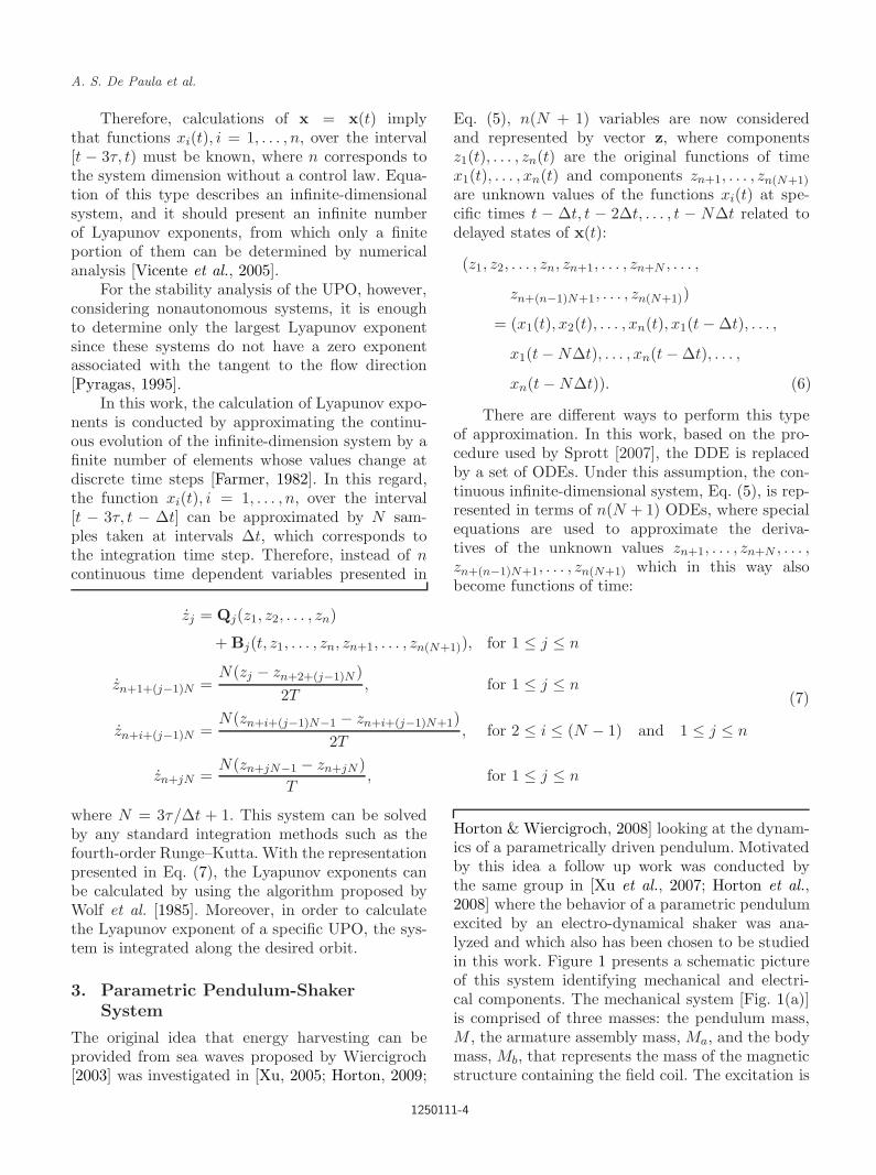
There are different ways to perform this typeof approximation. In this work, based on the pro-cedure used by Sprott [2007], the DDE is replacedby a set of ODEs. Under this assumption, the con-tinuous infinite-dimensional system, Eq. (5), is rep-resented in terms of n(N + 1) ODEs, where specialequations are used to approximate the deriva-tives of the unknown values zn+1, . . . , zn+N , . . . ,zn+(n−1)N+1, . . . , zn(N+1) which in this way alsobecome functions of time:

zj = Qj(z1, z2, . . . , zn)

+ Bj(t, z1, . . . , zn, zn+1, . . . , zn(N+1)), for 1 ≤ j ≤ n

zn+1+(j−1)N =N(zj − zn+2+(j−1)N )

2T, for 1 ≤ j ≤ n

zn+i+(j−1)N =N(zn+i+(j−1)N−1 − zn+i+(j−1)N+1)

2T, for 2 ≤ i ≤ (N − 1) and 1 ≤ j ≤ n

zn+jN =N(zn+jN−1 − zn+jN )

T, for 1 ≤ j ≤ n

(7)

where N = 3τ/∆t + 1. This system can be solvedby any standard integration methods such as thefourth-order Runge–Kutta. With the representationpresented in Eq. (7), the Lyapunov exponents canbe calculated by using the algorithm proposed byWolf et al. [1985]. Moreover, in order to calculatethe Lyapunov exponent of a specific UPO, the sys-tem is integrated along the desired orbit.

3. Parametric Pendulum-ShakerSystem

The original idea that energy harvesting can beprovided from sea waves proposed by Wiercigroch[2003] was investigated in [Xu, 2005; Horton, 2009;

Horton & Wiercigroch, 2008] looking at the dynam-ics of a parametrically driven pendulum. Motivatedby this idea a follow up work was conducted bythe same group in [Xu et al., 2007; Horton et al.,2008] where the behavior of a parametric pendulumexcited by an electro-dynamical shaker was ana-lyzed and which also has been chosen to be studiedin this work. Figure 1 presents a schematic pictureof this system identifying mechanical and electri-cal components. The mechanical system [Fig. 1(a)]is comprised of three masses: the pendulum mass,M , the armature assembly mass, Ma, and the bodymass, Mb, that represents the mass of the magneticstructure containing the field coil. The excitation is

1250111-4

June 19, 2012 18:5 WSPC/S0218-1274 1250111

Bifurcation Control of a Parametric Pendulum

bcbk

aM

bM

acakaX

bX

emF

mθ

cl

backE

EL

RI

E =- (X -X )κback ba

(a) (b)

Fig. 1. Physical model of the pendulum-shaker system with mechanical and electrical components. Adopted from [Xu et al.,2007].

provided by an axial electromagnetic force, Fem,which is generated by the alternating current in theconstant magnetic field.

The mechanical part of the pendulum-shakersystem is described by three generalized coordi-nates: angular displacement of the pendulum, θ,

and the vertical displacements of the body andthe armature, Xb and Xa, respectively. The elec-trical system is described by the electric charge q,that is related to the current I by its derivative:I = dq/dt. Equations of motion for each degree-of-freedom of the parametric pendulum-shaker systemare given by:

θ: Ml θ + clθ + Mg sin θ = MXa sin θ +TC

l,

Xa: (Ma + M)Xa + ca(Xa − Xb) + ka(Xa − Xb) = (Ma + M)g + Ml θ sin θ + Ml θ2 cos θ − κI,

Xb: MbXb + cbXb − ca(Xa − Xb) + kbXb − ka(Xa − Xb) = Mbg + κI, (8)

I: REI + LdI

dt− κ(Xa − Xb) = E0 cos Ωt,

where TC corresponds to the control parameter actuation, which consists of a torque applied to the pen-dulum. Considering the state variables x1, x2, x3, x4, x5, x6, x7 = θ, θ,Xa, Xa,Xb, Xb, I, the equationsof motion are now written as a set of first-order differential equations:

x1 = x2,

x2 =

(TC

l− clx2

)(Ma + M) − [ca(x4 − x6) + ka(x3 − x5) + κx7]M sinx1 + M2lx2

2 cos x1 sin x1

Ml(Ma + M − M sin2 x1),

x3 = x4,

x4 =(Ma + M)g + Mlx 2

2 cos x1 − κx7 − ca(x4 − x6) − ka(x3 − x5) − clx2 sin x1 − mg sin2 x1

Ma + M − M sin2 x1,

x5 = x6,

1250111-5

June 19, 2012 18:5 WSPC/S0218-1274 1250111

A. S. De Paula et al.

x6 =Mbg + κx7 − c6x6 + ca(x4 − x6) − kbx5 + ka(x3 − x5)

Mb,

x7 =E0 cos(Ωt) − REx7 + κ(x4 − x6)

L.

(9)

By using the formalism presented for theextended time-delayed feedback control law, thecontrol actuation TC , with Nτ = 3, may beexpressed as follows:

TC =Ml2(Ma + M − M sin2 x1)

(Ma + M)

×K[(1 − R)(xτ + Rx2τ + R2x3τ ) − x2],

(10)

where xτ = x2(t − τ), x2τ = x2(t − 2τ) andx3τ = x2(t−3τ). Moreover, matrix gain K becomesa scalar K once the control action is only appliedto one differential equation, the one related to timeevolution of x2, and its control law is only associ-ated with delayed values of one state variable, x2. Inother words, only component K22 is different fromzero and notation K is used for it. Therefore, inthis case only N new variables will be required toapproximate the values of x2(t) at the delayed statesas presented in Eq. (11).

z8 =N(z2 − z9)

2τ

zj =N(zi−1 − zi+1)

2τ, if 9 ≤ i < N + 7 (11)

zN+7 =N(zN+6 − zN+7)

τ

where z8(t), . . . , zN+7(t) correspond to delayedstates of x2(t) and z1(t), . . . , z7(t) correspond tox1(t), . . . , x7(t).

Xu et al. [2007] discussed experimental aspectsof the pendulum-shaker dynamics. Here, we use theproposed model with experimentally determinedparameters presented in Table 1.

Table 1. Experimentally determined parameters of thependulum-shaker system [Xu et al., 2007].

M 0.845 kg l 0.3166 m c 0.0475 kg/s

Ma 68.38 kg ka 86175.9 kg/s2 ca 534.05 kg/s

Mb 820 kg kb 244284 kg/s2 cb 679.35 kg/s

RE 0.3 Ω L 2.626 × 10−3 H κ 130 N/A

At this point, let us briefly analyze the uncon-trolled system behavior. Bifurcation diagrams areconstructed by assuming a quasi-static strobo-scopic increase of the voltage amplitude E0 withinitial value of E0 = 60 V. The first 200 periodsare neglected in order to reach the steady stateresponse. The diagram in Fig. 2(a) shows perioddoubling bifurcations that lead to chaotic regionsand then, periodic window with a period-6 response.It is calculated for Ω = 9 rad/s, whereas a Poincare

(a)

(b)

Fig. 2. (a) Bifurcation diagram constructed at Ω = 9 rad/sand (b) Poincare section at E0 = 115 V.

1250111-6

June 19, 2012 18:5 WSPC/S0218-1274 1250111

Bifurcation Control of a Parametric Pendulum

section of the chaotic attractor is shown inFig. 2(b) for E0 = 115 V [marked by pink linein Fig. 2(a)] considering the phase space boundedwithin (−π,+π).

In order to explore some details of the dynam-ical behavior of the pendulum-shaker system, adifferent bifurcation diagram is now constructed

Fig. 3. Bifurcation diagram at E0 = 85 V calculated by increasing and decreasing the forcing frequency. Different coexistingsolutions are highlighted.

under the variation of frequency parameter Ω andE0 = 85 V. Figure 3 presents three different sit-uations: increasing the forcing frequency, in pink,and decreasing the frequency with different initialconditions, in black and in gray. The analysis ofFig. 3 shows that the system seems to have similarbehavior at Ω = 12.2 rad/s and Ω = 10.25 rad/s.

1250111-7

June 19, 2012 18:5 WSPC/S0218-1274 1250111

A. S. De Paula et al.

Nevertheless, in the first case the system presentsthree coexisting periodic attractors, while at Ω =10.25 rad/s, there are two quasi-periodic and oneperiodic attractors coexisting. The phase space ofthe coexisting orbits at Ω = 12.2 rad/s, two period-1and one period-2, and at Ω = 10.25 rad/s, twoquasi-periodic and one period-2, are depicted inFig. 3.

The analysis of the system dynamics showsthat the parametric pendulum may present dif-ferent kinds of solutions. Periodic, quasi-periodicand chaotic responses are all present in the sys-tem behavior. Besides, it is important to highlightthe coexisting attractors that can occur for thesame set of parameters. Therefore, bifurcation con-trol is important when we are thinking of the useof this pendulum system in some application. Interms of energy harvesting, it is of special interestto keep a period-1 rotating orbit, avoiding any kindof bifurcation. Another interesting procedure couldbe the stabilization of a rotation solution immersedin chaotic attractor. In this regard, we will applycontrol techniques for bifurcation control.

4. Controlling the Pendulum-ShakerSystem

In this section, continuous chaos control methodsare employed in order to stabilize unstable peri-odic orbits. Different scenarios are considered. First,classical chaos control is performed, stabilizing someUPOs embedded in chaotic attractor. Then, perioddoubling bifurcation is avoided in order to keepa period-1 rotating orbit. Finally, bifurcation to

chaos is prevented by stabilizing originally unsta-ble period-1 rotating orbit. All these scenarios areimportant for energy harvesting purposes.

4.1. Chaos control

In this subsection, continuous chaos controlapproach is employed in order to stabilize someUPOs of the pendulum-shaker system. The firststep of this control is the learning stage whereUPO is identified and control parameters are cho-sen. Figure 4(a) presents a period-1 UPO identi-fied by the close return method [Auerbach et al.,1987] at Ω = 9 rad/s and E0 = 115 V, related to thePoincare section presented in Fig. 2. Figure 4(b)shows its largest Lyapunov exponents consideringdifferent control parameters. It is important to high-light that in Lyapunov exponent calculation, as wellas in the control stage, the value of τ is equal to theperiodicity of the desired UPO. The analysis of thecontrol parameters shows that there are differentalternatives to obtain negative values of Lyapunovexponents and these values can be used for controlpurposes.

Control is now applied with the purpose tostabilize the period-1 UPO (rotating solution)assuming R = 0 and K = 1.2. Figure 5 showspendulum displacement and applied torque evolu-tion in time. The initial function x0 = x0(t) overthe time interval [−Nττ, 0) is estimated by theTaylor series expansion presented in Eq. (3) andx0(0) = −3, 0, . . . , 0. Figure 6 presents pendulumphase space during the control period highlightingthe steady-state response (in pink).

(a) (b)

Fig. 4. (a) Period-1 UPO, (b) its largest Lyapunov exponent for different values of the control parameters K and R.

1250111-8

June 19, 2012 18:5 WSPC/S0218-1274 1250111

Bifurcation Control of a Parametric Pendulum

(a) (b)

Fig. 5. Period-1 UPO stabilized for R = 0, K = 1.2 and x0(0) = −3, 0, . . . , 0: (a) time response, (b) applied torque.

4.2. Control to avoid perioddoubling bifurcation

If the system is required to operate in a stablerotational mode, the qualitative changes in systemresponse must be avoided over the extended param-eter range. The bifurcations of the system can beprevented if chaos control methods are applied. Fig-ure 7(a) shows a period-1 orbit for E0 = 95.5 V andΩ = 9 rad/s, before the period doubling bifurca-tion, while Fig. 7(b) presents the largest Lyapunovexponent of this orbit for different control param-eters, Ω = 9 rad/s and E0 = 96 V, a value afterthe period doubling bifurcation. Figure 8 shows thebifurcation diagram of pendulum displacement atΩ = 9 rad/s without control action (black) and withcontrol action (pink) considering two different sets

Fig. 6. Phase space controlled response for R = 0, K =1.2 and x0(0) = −3, 0, . . . , 0. The steady state response ismarked in pink.

of control parameters: R = 0, K = 0.6 and R = 0,K = 1. Note that bifurcation is avoided in bothcases but the second case is more effective to main-tain the period-1 response.

In this work, the control parameters associatedwith the minimum value of the largest Lyapunovexponent are chosen to stabilize the system [Pyra-gas, 1995]. In Fig. 7(b), however, it can be observedthat the same minimum value of Lyapunov expo-nent is obtained for 0.5 < K < 1.1 and R = 0.When the different values of K, with R = 0, areused to perform the bifurcation control, the largervalues of K lead to a more effective control, whichmeans that stability of the rotational solution ismaintained over larger range of E0. This can beseen from Fig. 8(b), where for K = 1, the period-1rotational orbit remains stable for the whole rangeof the analyzed E0. Therefore, in this case the opti-mal value of K can be chosen depending on theconsidered voltage amplitude range to avoid unnec-essary high control effort.

It is important to mention that the periodicorbits presented in Fig. 8 in pink are obtained bystabilizing the unstable periodic orbits of the orig-inal system. Therefore, the variation of the param-eter E0 induces a change in the response which iscompensated by the control action. Figure 9 showsthe time history of applied torque under the per-formed perturbations, encompassing three increasesof the value of E0. Note that the variation of theparameter E0 is related to a transient response ofthe controller, and after each increase in E0, a rel-atively small control action is required to stabi-lize the desired periodic orbit, but once it is done,

1250111-9

June 19, 2012 18:5 WSPC/S0218-1274 1250111

A. S. De Paula et al.

(a) (b)

Fig. 7. (a) Period-1 orbit pendulum response for E0 = 95.5 V, (b) its largest Lyapunov exponent for E0 = 96 V and differentcontrol parameters.

(a) (b)

Fig. 8. Bifurcation diagram at Ω = 9 rad/s without control action (black) and with control action (pink): (a) R = 0 andK = 0.6, (b) R = 0 and K = 1.

Fig. 9. Detail of the performed control action in bifurcationcontrol.

there is little control effort needed to maintain thisregime.

4.3. Control to avoid bifurcation tochaos — Preserving rotatingorbits

A different possibility concerning the control of thependulum-shaker system is to avoid the chaoticbehavior and to maintain the period-1 rotatingresponse. Figure 10 presents some coexisting orbitsidentified in the bifurcation diagram of Fig. 3.Figure 10(a) presents a phase space with threeorbits: two rotating period-1 orbits and an oscillat-ing period-2 orbit that coexists at Ω = 12.2 rad/sand E0 = 85 V. Figure 10(b) presents the phase

1250111-10

June 19, 2012 18:5 WSPC/S0218-1274 1250111

Bifurcation Control of a Parametric Pendulum

(a) (b)

Fig. 10. Phase space of coexisting attractors: (a) three periodic regimes at E0 = 85 V and Ω = 12.2 rad/s, (b) one periodicand two quasi-periodic regimes, together with their Poincare sections, at E0 = 85V and Ω = 10.25 rad/s.

space of the same orbits at Ω = 10.25 rad/s andE0 = 85 V showing the change of the two period-1rotating orbits for two quasi-periodic rotatingorbits. This picture also presents the Poincare sec-tions of quasi-periodic responses.

The control is now applied to these orbits, andthe case where the forcing frequency is decreasingis considered. The aim is to maintain a rotatingorbit, avoiding the bifurcation to chaos. Moreover,since the period-2 orbit is not a rotating orbit,this response is not desirable. Decreasing the fre-quency, the system presents the following routeto chaos: period-1 orbit, then quasi-periodic orbitand then chaos. Before the bifurcation to chaosthe system presents a quasi-periodic behavior, theperiod-1 “positive” orbit identified at E0 = 85 Vand Ω = 12.2 rad/s is considered as the fiducialtrajectory. Figure 11 presents the largest Lyapunovexponent of this orbit for different control param-eters at E0 = 85 V and Ω = 10.335 rad/s, a set ofparameters related to chaotic behavior.

After the learning stage, control is applied tothe system. Figure 12 shows the bifurcation dia-gram constructed at E0 = 85 V with and with-out control action. Controller uses R = 0.2 andK = 0.4 with the objective of keep the rotatingresponse of the system. At first, the controller waitsuntil the system trajectory “falls” in the neighbor-hood of the desired orbit to be in the control onmode [Fig. 12(a)]. In other words, the system isintegrated without control action until its trajec-tory goes into the neighborhood of the desired UPO.When this neighborhood, defined by considering

a given tolerance, is reached the control actionbegins. This wait time is necessary due to the quasi-periodic behavior. If this wait time is not consideredand the control action begins in the first integra-tion time step, the controller is not able to stabi-lize the desired orbit as shown in Fig. 12(b). Thiswait time is an essential characteristic of discretechaos control method [Ott et al., 1990; Hubingeret al., 1994; De Paula & Savi, 2008, 2009a] usuallynot being employed in continuous methods [Pyra-gas, 1992; Socolar et al., 1994; De Paula & Savi,2009b].

Figure 13 presents the controlled orbit after thewait time for E0 = 85 V and two different situations:Ω = 10.3 rad/s and Ω = 10.15 rad/s. It is clear that

Fig. 11. Largest Lyapunov exponent of the period-1 orbitat E0 = 85 V and Ω = 10.335 rad/s for different values of Rand K.

1250111-11

June 19, 2012 18:5 WSPC/S0218-1274 1250111

A. S. De Paula et al.

(a) (b)

Fig. 12. Bifurcation diagram at E0 = 85V with and without control: (a) with a wait time, (b) without a wait time.

(a) (b)

Fig. 13. Steady state response of the controlled system for E0 = 85 V. (a) Ω = 10.3 rad/s, (b) Ω = 10.15 rad/s.

chaotic motion is avoided as well as period-2 orbit.Nevertheless, it should be pointed out that the con-trolled response is a quasi-periodic behavior.

5. Conclusions

This paper presents the modeling and analysis ofbifurcation control of a pendulum-shaker system.This electro-mechanical system may be used to sim-ulate the dynamics of a pendulum system usedto explore the concept of energy harvesting fromsea waves. This idea requires the rotating periodicresponse of the system to be maintained throughouta significant parameters range. The bifurcation con-trol is applied in order to stabilize desired rotational

orbits for the parameter values where they are orig-inally unstable.

The continuous control method known asextended time delayed feedback is employed and dif-ferent scenarios are investigated. First, the classicalchaos control is realized, where some UPOs embed-ded in chaotic attractor are stabilized. Then perioddoubling bifurcation is prevented in order to main-tain a period-1 rotating orbit. Finally, bifurcationto chaos is avoided and a stable rotating solution ismaintained.

Acknowledgments

The authors would like to thank the Brazil-ian Research Agencies CNPq and FAPERJ and

1250111-12

June 19, 2012 18:5 WSPC/S0218-1274 1250111

Bifurcation Control of a Parametric Pendulum

through the INCT-EIE (National Institute ofScience and Technology — Smart Structures inEngineering) the CNPq and FAPEMIG for theirsupport. The Air Force Office of Scientific Research(AFOSR) is also acknowledged.

References

Abed, E. H. & Fu, J.-H. [1986] “Local feedback stabi-lization and bifurcation control, I. Hopf bifurcation,”Syst. Contr. Lett. 7, 11–17.

Abed, E. H. & Fu, J.-H. [1987] “Local feedback stabi-lization and bifurcation control, II. Stationary bifur-cation,” Syst. Contr. Lett. 8, 467–473.

Auerbach, D., Cvitanovic, P., Eckmann, J.-P.,Gunaratne, G. & Procaccia, I. [1987] “Exploringchaotic motion through periodic orbits,” Phys. Rev.Lett. 58, 2387–2389.

Bishop, S. R., Sofroniou, A. & Shi, P. [2005] “Symmetry-breaking in the response of the parametrically excitedpendulum model,” Chaos Solit. Fract. 25, 257–264.

Capecchi, D. & Bishop, S. [1990] “Periodic and non-periodic responses of a parametrically excited pendu-lum,” Report 3/90 of the Dipartimento di Ingegneriadelle Strutture, delle Acque e del Terreno, UniversitadellAquila, Italy.

Chen, G., Moiola, J. L. & Wang, H. O. [2000] “Bifur-cation control: Theories, method, and applications,”Int. J. Bifurcation and Chaos 10, 511–548.

Chen, G., Hill, D. & Yu, X. [2003] Bifurcation Control:Theory and Applications (Springer, Berlin), pp. 99–126.

Clifford, M. J. & Bishop, S. R. [1994] “Approximatingthe escape zone for the parametrically excited pendu-lum,” J. Sound Vib. 172, 572–576.

Clifford, M. J. & Bishop, S. R. [1995] “Rotating periodicorbits of the parametrically excited pendulum,” Phys.Lett. A 201, 191–196.

Clifford, M. J. & Bishop, S. R. [1996] “Locating oscilla-troy orbits of the parametrically-excited pendulum,”J. Aust. Math. Soc. Ser. B — Appl. Math. 37,309–319.

Cunningham, W. J. [1954] “A nonlinear differential-difference equation of growth,” Mathematics 40,708–713.

De Paula, A. S. & Savi, M. A. [2008] “A multiparameterchaos control method applied to maps,” Brazilian J.Phys. 38, 537–543.

De Paula, A. S. & Savi, M. A. [2009a] “A multiparam-eter chaos control method based on OGY approach,”Chaos Solit. Fract. 40, 1376–1390.

De Paula, A. S. & Savi, M. A. [2009b] “Controlling chaosin a nonlinear pendulum using an extended time-delayed feedback control method,” Chaos Solit. Fract.42, 2981–2988.

Farmer, J. D. [1982] “Chaotic attractors of an infinite-dimensional dynamical system,” Physica D 4, 366–393.

Garira, W. & Bishop, S. R. [2003] “Rotating solutions ofthe parametrically excited pendulum,” J. Sound Vib.263, 233–239.

Horton, B. W. & Wiercigroch, M. [2008] “Effects of heaveexcitation on rotations of a pendulum for wave energyextraction,” IUTAM Symp. Fluid-Structure Interac-tion Ocean Eng. 8, 117–128.

Horton, B. W., Wiercigroch, M. & Xu, X. [2008] “Tran-sient tumbling chaos and damping identification forparametric pendulum,” Phil. Trans. Roy. Soc. A —Math. Phys. Eng. Sci. 366, 767–784.

Horton, B. W. [2009] Rotational Motion of Pendula Sys-tems for Wave Energy Extraction, PhD thesis, Uni-versity of Aberdeen.

Horton, B. W., Sieber, J., Thompson, J. M. T. & Wierci-groch, M. [2011] “Dynamics of the nearly parametricpendulum,” Int. J. Nonlin. Mech. 46, 436–442.

Hubinger, B., Doerner, R., Martienssen, W., Herder-ing, M., Pitka, R. & Dressler, U. [1994] “Control-ling chaos experimentally in systems exhibiting largeeffective Lyapunov exponents,” Phys. Rev. E 50,932–948.

Kittel, A., Parisi, J. & Pyragas, K. [1995] “Delayed feed-back control of chaos by self-adapted delay time,”Phys. Lett. A 198, 433–436.

Koch, B. P. & Leven, R. W. [1985] “Subharmonic andhomoclinic bifurcations in a parametrically forcedpendulum,” Physica D 16, 1–13.

Lenci, S., Pavlovskaia, E., Rega, G. & Wiercigroch, M.[2008] “Rotating solutions and stability of parametricpendulum by perturbation method,” J. Sound Vib.310, 243–259.

Mensour, B. & Longtin, A. [1997] “Power spectra anddynamical invariants for delay-differential and differ-ence equations,” Physica D 113, 1–25.

Ott, E., Grebogi, C. & Yorke, J. A. [1990] “ControllingChaos,” Phys. Rev. Lett. 64, 1196–1199.

Pyragas, K. [1992] “Continuous control of chaos byself-controlling feedback,” Phys. Lett. A 170, 421–428.

Pyragas, K. [1993] “Predictable chaos in slightly per-turbed unpredictable chaotic systems,” Phys. Lett. A181, 203–210.

Pyragas, K. [1995] “Control of chaos via extended delayfeedback,” Phys. Lett. A 206, 323–330.

Pyragas, K. [2006] “Delayed feedback control of chaos,”Phil. Trans. Roy. Soc. A 364, 2309–2334.

Socolar, J. E. S., Sukow, D. W. & Gauthier, D. J. [1994]“Stabilizing unstable periodic orbits in fast dynamicalsystems,” Phys. Rev. E 50, 3245–3248.

Sprott, J. C. [2007] “A simple chaotic delay differentialequation,” Phys. Lett. A 366, 397–402.

1250111-13

June 19, 2012 18:5 WSPC/S0218-1274 1250111

A. S. De Paula et al.

Szemplinska-Stupnicka, W., Tyrkiel, E. & Zubrzycki, A.[2000] “The global bifurcations that lead to transienttumbling chaos in a parametrically driven pendulum,”Int. J. Bifurcation and Chaos 10, 2161–2175.

Szemplinska-Stupnicka, W. & Tyrkiel, E. [2002] “Theoscillation-rotation attractors in the forced pendulumand their peculiar properties,” Int. J. Bifurcation andChaos 12, 159–168.

Vicente, R., Daudn, J., Colet, P. & Toral, R. [2005]“Analysis and characterization of the hyperchaos gen-erated by a semiconductor laser subject to a delayedfeedback loop,” IEEE J. Quant. Electron. 41, 541–548.

Wen, G., Wang, Q.-G. & Chin, M.-S. [2006] “Delay feed-back control for interaction of Hopf and period dou-bling bifurcations in discrete-time systems,” Int. J.Bifurcation and Chaos 16, 101–112.

Wiercigroch, M. [2003] A New Concept of Energy Extrac-tion from Waves via Parametric Pendulor, personalcommunications.

Wolf, A., Swift, J. B., Swinney, H. L. & Vastano, J. A.[1985] “Determining Lyapunov exponents from a timeseries,” Physica D 16, 285–317.

Xiao, M. & Cao, J. [2009] “Delayed feedback-basedbifurcation control in an Internet congestion model,”J. Math. Anal. Appl. 332, 1010–1027.

Xu, X. [2005] Nonlinear Dynamics of Parametric Pen-dulum for Wave Energy Extraction, PhD thesis, Uni-versity of Aberdeen.

Xu, X., Wiercigroch, M. & Cartmell, M. P. [2005]“Rotating orbits of a parametrically-excited pendu-lum,” Chaos Solit. Fract. 23, 1537–1548.

Xu, X. & Wiercigroch, M. [2007] “Approximate analyt-ical solutions for oscillatory and rotational motionof a parametric pendulum,” Nonlin. Dyn. 47,311–320.

Xu, X., Pavlovskaia, E., Wiercigroch, M., Romeo, F. &Lenci, S. [2007] “Dynamic interactions between para-metric pendulum and electro-dynamical shaker,” Z.Angew. Math. Mech. 87, 172–186.

1250111-14