mathematics

Article

Computational Analysis and Bifurcation of Regular andChaotic Ca2+ Oscillations

Xinxin Qie and Quanbao Ji *

�����������������

Citation: Qie, X.; Ji, Q.

Computational Analysis and

Bifurcation of Regular and Chaotic

Ca2+ Oscillations. Mathematics 2021, 9,

3324. https://doi.org/10.3390/

math9243324

Academic Editors: Youming Lei and

Lijun Pei

Received: 18 November 2021

Accepted: 17 December 2021

Published: 20 December 2021

Publisher’s Note: MDPI stays neutral

with regard to jurisdictional claims in

published maps and institutional affil-

iations.

Copyright: © 2021 by the authors.

Licensee MDPI, Basel, Switzerland.

This article is an open access article

distributed under the terms and

conditions of the Creative Commons

Attribution (CC BY) license (https://

creativecommons.org/licenses/by/

4.0/).

School of Mathematics and Physics, Guangxi University for Nationalities, Nanning 530006, China;q_740289128@163.com* Correspondence: jqb_2001@163.com

Abstract: This study investigated the stability and bifurcation of a nonlinear system model developedby Marhl et al. based on the total Ca2+ concentration among three different Ca2+ stores. In thisstudy, qualitative theories of center manifold and bifurcation were used to analyze the stability ofequilibria. The bifurcation parameter drove the system to undergo two supercritical bifurcations. Itwas hypothesized that the appearance and disappearance of Ca2+ oscillations are driven by them.At the same time, saddle-node bifurcation and torus bifurcation were also found in the process ofexploring bifurcation. Finally, numerical simulation was carried out to determine the validity of theproposed approach by drawing bifurcation diagrams, time series, phase portraits, etc.

Keywords: bifurcation; chaos; hopf bifurcation; center manifold

1. Introduction

Ca2+ is one of the vital ions for information processing in humans. It generally actsas a biological messenger in different cell types and is an indispensable ion for variousphysiological activities in the human body [1–4]. Ca2+ plays a particularly importantrole in the regulation and control of body functions. It is involved in the mechanism ofheartbeat and thrombin formation, but also transmits neural signaling, modifies the enzymeactivity, and regulates the mechanisms underlying the maturation and fertilization of germcells. A phenomenon observed experimentally in most cell types is that intracellular Ca2+

concentration remains stable without stimulation. Some Ca2+ enter the cytosol from theCa2+ store when the cell is stimulated, leading to an increment in Ca2+ concentration thattriggers a series of physiological activities [5–13]. The cell adjusts itself and closes theCa2+ channels when the stimulation increases to a certain extent, and then Ca2+ is takenup by Ca2+ stores. After a while, the intracellular Ca2+ concentration gains stability, andthe cell returns to a resting state. The source of intracellular Ca2+ is mainly through theinflux of extracellular Ca2+ and the release of Ca2+ stored in the endoplasmic reticulumor sarcoplasmic reticulum. The latter is mainly based on the mechanism of Ca2+ releasefrom intracellular Ca2+ stores triggered by Ca2+ signaling, namely Ca2+-induced Ca2+

release [14–16].Over the past few years, many investigations have been carried out on evoked Ca2+

dynamics. Oscillations of free Ca2+ concentrations are highly significant and ubiquitouscontrol mechanisms in a large number of cells. Experimental evidence has demonstratedthat Ca2+ oscillations have different characteristics such as regularity and chaos. Chaosrefers to dynamic systems that are sensitive to initial values, resulting in unpredictablerandom motion. Chaotic motion has been associated with making long-term weatherpredictions and the discovery of Lorentz attractors. In physiology, various arrhythmias,atrioventricular block, and ventricular fibrillation may also be associated with chaos. Awell-known manifestation of chaos is the butterfly effect. This refers to a small changethat brings about widely varying consequences for the future as it continues to pass andhas long been applied to the weather and the stock market. In psychology, for example,

Mathematics 2021, 9, 3324. https://doi.org/10.3390/math9243324 https://www.mdpi.com/journal/mathematics

Mathematics 2021, 9, 3324 2 of 17

when a person receives a small psychological stimulus in childhood, as they grow older,this stimulus can have a large impact on them in adulthood. In addition, the approachto chaos mainly consists of period doubling bifurcations, quasi-periodic transitions, andintermittent chaos. The period doubling bifurcation can be seen in the bifurcation diagram.

After the discovery of oscillations by Wood et al. [17,18], Ca2+ oscillations have beenextensively studied. Ca2+ oscillations can be classified into two types: the first type is simpleCa2+ oscillations, and the second is bursting. Simple Ca2+ oscillations have been exploredextensively. In the experiments of Borghans et al. (1997), some more complex forms ofCa2+ oscillations have been found such as bursts and chaos. When the system enterschaos, the Ca2+ oscillations show an extremely sensitive dependence on the initial value.Borghans et al. and Houart et al. further proposed several possible mechanisms to explainthe complex intracellular Ca2+ oscillations and performed mathematical analysis [19,20].Chay also proposed a model for Ca2+ oscillations in excitable cells [21], and Shen andLarter (1995) studied complex Ca2+ oscillations and chaotic phenomena in non-excitablecells [22,23]. In these models, it is almost certain that the burst results from changes inIP3 yields because IP3 can stimulate Ca2+ channels and release a large number of Ca2+

into the cytosol or take up Ca2+ from the cytosol, thereby participating in Ca2+ regulation.This is one of the most straightforward explanations for the bursting of intracellularCa2+. One mechanism proposed by Borghans et al. to explain complex Ca2+ oscillationsis that bursting oscillations are associated with Ca2+-releasing channel activities in theendoplasmic reticulum. A further mechanism investigated in the same study is that thereis not just one intracellular Ca2+ store. Both IP3-sensitive and non-sensitive Ca2+ storeshave been taken into account. In all models, the endoplasmic reticulum is the primary Ca2+

store for intracellular Ca2+.Marhl et al. suggested the significance of free Ca2+ concentrations in mitochondria for

Ca2+ oscillations and proposed a likely explanation for Ca2+ oscillations in cells [24]. In thisstudy, the model focuses on Ca2+ exchange in the middle of the cytosol, endoplasmic retic-ulum, and mitochondria. The Ca2+ considered in the model includes cytosol, endoplasmicreticulum, and mitochondrial Ca2+ [25,26] and binds Ca2+ in the cytosol. These modelswell simulate enriched Ca2+ oscillations in cells. Nevertheless, in past investigations, thechanges induced by different values of Catot have not been discussed in detail. Moreover,most of the literature has focused on experiments, rarely analyzing the principles of Ca2+

oscillations theoretically. Therefore, this study takes Marhl et al.’s Ca2+ oscillation modelas the research object, selects Catot as a bifurcation parameter, analyzes the features ofequilibrium by the qualitative theory of differential equation, and discusses the bifurcationof equilibrium by the bifurcation and center manifold theory [27–30]. The qualitativetheory of differential equations allows for analysis of the characteristics of the equilibriumpoint of the system including stability, coordinates, and types. Specifically, the analysis wasconducted using eigenvalues and the Hurwitz criterion. In addition, when investigatingthe bifurcation of higher-order nonlinear dynamic systems, the center manifold theory cantransform the study of various behaviors of n-dimensional dynamic systems approach-ing equilibrium into the study of equations on m-dimensional (m < n) center manifolds,simplifying the system. Finally, the model was simulated numerically using AUTO andMATLAB in this study. The advantage is that it confirms our conclusions [31,32].

2. Description of the Model

The model established by Marhl et al. investigated the oscillation of free Ca2+ con-centrations in the cytosol, endoplasmic reticulum, and mitochondria. A mathematicalmodel was established to simulate the oscillation of intracellular Ca2+ concentration, andthe specific system is as follows [24]:

dCacytdt = Jch + Jleak + Jout − Jpump − Jin + k−CaPr− k+CacytPr

dCaerdt = βer

ρer(Jpump − Jch − Jleak)

dCamdt = βm

ρm(Jin − Jout)

, (1)

Mathematics 2021, 9, 3324 3 of 17

where Cacyt is the cytosolic Ca2+ concentration; Caer is the Ca2+ concentration in the en-doplasmic reticulum; Cam is the Ca2+ concentration in mitochondria; and Catot is theconservation of total extracellular Ca2+. Details of the specific meaning and value of eachparameter can be referred to in Table 1 and [24]. These parameters have the followingrelationships:

Jpump = kpumpCacyt, Prtot = Pr + CaPr, Jout = (koutCacyt2

K23+Cacyt2

+ km )Cam, Jin = kinCacyt8

K82+Cacyt8

,

Jch = kchCacyt

2

K21+Cacyt2

(Caer − Cacyt

), CaPr = Catot − Cacyt − ρer

βerCaer − ρm

βmCam,

Jleak = kleak(Caer − Cacyt

).

Table 1. Unless otherwise specified, the parameter values are used as given in this model.

Prtot 120 µM kpump 20 s−1

ρer 0.01 kout 125 s−1

ρm 0.01 km 0.00625 s−1

βer 0.0025 k− 0.01 s−1

βm 0.0025 K1 5 µMkch 1500 s−1 K2 0.8 µM

kleak 0.05 s−1 K3 5 µMkin 300 µM−1 s−1 k+ 0.1 µM−1 s−1

3. Results3.1. Analysis of Stability

Catot corresponds to the total intracellular Ca2+ concentration including free Ca2+ inthe cytosol, endoplasmic reticulum, and mitochondria. The model ignores the exchangebetween extracellular and cytosolic Ca2+ and focuses on the regulation of Ca2+ concentra-tion in the cytosol and organelles. In cells, Ca2+ generally exists in the organelles as freeor protein-bound. Ca2+ can be induced to increase or decrease either by binding to bufferproteins or by the dissociation of binding Ca2+.

There are two principal ways in which Ca2+ is regulated: absorption and liberationof Ca2+ by the endoplasmic reticulum and mitochondria. Therefore, during the process, aseries of experimental manipulations can be carried out to change the Ca2+ concentrationin organelles. Then, Catot will be changed in value. For example, intracellular injection ofIP3 leads to the liberation of Ca2+ in the endoplasmic reticulum, or Ca2+ pump inhibitorsare used to inhibit Ca2+ uptake from the endoplasmic reticulum, thereby increasing freecytosolic Ca2+. Based on the above reasons, Catot is a reasonable selection as the parameterthat can be changed in the experiment. This is a practical guide for the experiment.Therefore, Catot was chosen as the bifurcation parameter to discuss the existence, quantity,type, and bifurcation of the equilibrium.

To make the calculations easier, we can make x = Cacyt, y = Caer, z = Cam, r = Catot.Therefore, model (1) can be transformed into the following expression:

dxdt = 0.01r + 0.01y− 20.06x− 0.04z− 0.1x(x− r + 4y + 4z + 120)

− 1500x2(x−y)x2+25 − 300x8

x8+0.16777216 + z( 125x2

x2+25 + 0.00625)dydt = 5.0125x− 0.0125y + 375x2(x−y)

x2+25dzdt = −0.25z( 125x2

x2+25 + 0.00625) + 75x8

x8+0.16777216

. (2)

One can immediately see that the equilibrium point of system (2) meets the following equation:0.01r− 20.06x + 0.01y− 0.04z− 0.1x(x− r + 4y + 4z + 120)− 1500x2(x−y)

x2+25− 300x8

x8+0.16777216 + z( 125x2

x2+25 + 0.00625) = 0

5.0125x− 0.0125y + 375x2(x−y)x2+25 = 0

−0.25z( 125x2

x2+25 + 0.00625) + 75x8

x8+0.16777216 = 0

(3)

Mathematics 2021, 9, 3324 4 of 17

First, by calculating

− 0.25z(125x2

x2 + 25+ 0.00625) +

75x8

x8 + 0.16777216= 0,

we can obtain

z =75x8

( 31.25x2

x2+25 + 0.0015625)(x8 + 0.167772).

Then,

5.0125x− 0.0125y +375x2(x− y)

x2 + 25= 0

can be calculated to obtain

y =30401x3 + 10025x

30001x2 + 25.

Consequently, substituting the expression for y and z obtains

0.01r− 20.06x + 0.01y− 0.04z− 0.1x(x− r + 4y + 4z + 120)− 1500x2(x−y)x2+25

− 300x8

x8+0.16777216 + z( 125x2

x2+25 + 0.00625) = 0.

Therefore, we have the following equation:

f (x, r) = 0.01r− 20.06x− 0.1x(x− r + 4σ2σ3

+ 300x8

σ1+ 120)− 3x8

σ1+ 0.01σ2

σ3

− 300x8

x8+0.16777216 −1500x2(x− σ2

σ3)

x2+25 +75x8( 125x2

x2+25+0.00625)

σ1= 0

y = 30401x3+10025x30001x2+25

z = 75x8

σ1

, (4)

where

σ1 = (31.25x2

x2 + 25+ 0.0015625)(x8 + 0.167772), σ2 = 30401x3 + 10025x, σ3 = 30001x2 + 25.

Depending on the practical implications of x, y, z, and r, whether Equation (2) has anequilibrium point was considered to meet our special needs when r ∈ [0, 150]. Suppose(x0, y0, z0) is equilibrium. Let x1 = x − x0, y1 = y − y0, z1 = z − z0, then we can obtain thefollowing representations [30]:

dx1dt = 0.01r− 20.06(x1 + x0) + 0.01(y1 + y0)− 0.04(z1 + z0)− 0.1(x1 + x0)(4(y1

+y0) + 4(z1 + z0) + 120 + x1 + x0 − r)− 1500(x1+x0)2(x1+x0−y1−y0)

(x1+x0)2+25

− 300(x1+x0)8

(x1+x0)8+0.16777216

+ z(

125(x1+x0)2+0.00625((x1+x0)

2+25)(x1+x0)

2+25

)dy1dt = −0.0125(y1 + y0) + 5.0125(x1 + x0) +

375(x1+x0)2(x1+x0−y1−y0)

(x1+x0)2+25

dz1dt = 75(x1+x0)

8

(x1+x0)8+0.16777216

− 0.25(z1 + z0)

(125(x1+x0)

2

(x1+x0)2+25

+ 0.00625)

. (5)

Obviously, (0, 0, 0) is the equilibrium of system (5), which, according to bifurcationtheory, has the same features as that of the equilibrium of system (2) in terms of type,stability, and bifurcation type. The Jacobian matrix of system (5) can be easily calculatedas follows:

J = (bij)3×3 =

b11 b12 b13b21 b22 b23b31 b32 b33

.

Mathematics 2021, 9, 3324 5 of 17

The linearized system corresponding to the equilibrium (0, 0, 0) of system (5) isdx1dt = b11x1 + b12y1 + b13z1

dy1dt = b21x1 + b22y1 + b23z1

dz1dt = b31x1 + b32y1 + b33z1

,

where

b11 = 0.1r− 0.2x0 − 0.4y0 − 0.4z0 − 32.06− 2400x07

x08+0.16777216 + 2400x0

15

(x08+0.16777216)2 +

z0(250x0

x02+25 −

250x03

(x02+25)2 )− 1500x0

2

x02+25 −

3000x0(x0−y0)x0

2+25 + 3000x03(x0−y0)

(x02+25)2 ,

b12 = −0.4x0 + 0.01 + 1500x02

x02+25 , b13 = −0.4x0 − 0.03375 + 125x0

2

x02+25 ,

b21 = 5.0125 + 375x02

x02+25 + 750x0(x0−y0)

x02+25 − 750x0

3(x0−y0)

(x02+25)2 , b22 = −0.0125− 375x0

2

x02+25 ,

b23 = 0, b31 = 600x07

x08+0.16777216 −

600x015

(x08+0.16777216)2 − 0.25z0(

250x0x0

2+25 −250x0

3

(x02+25)2 ),

b32 = 0, b33 = −0.0015625− 31.25x02

x02+25 .

There is also a simple way to obtain the following eigen equation of the Jacobianmatrix:

P(λ) = λ3 + C1λ2 + C2λ + C3 = 0,

where

C1 = −b11 − b22 − b33,C2 = b11b22 + b11b33 + b22b33 − b13b31 − b12b21 − b32b23,C3 = b31b13b22 + b12b21b33 + b32b23b11 − b11b22b33 − b12b23b31 − b13b21b32.

The following formula is obtained by calculating:

C1 = −0.1r + 0.2x0 + 0.4y0 + 0.4z0 +2400x7

0x8

0+0.16777216− 2400x15

0σ4− z0σ5 +

1906.25x20

x20+25

+32.0740625 + 3000x0(x0−y0)

x20+25

− 3000x30(x0−y0)σ6

,

C2 = (σ3 + 0.0125)σ7 + σ1σ7 + (σ3 + 0.0125)σ1 − (σ2 − 0.4x0 + 0.01)(σ3 +750x0(x0−y0)

x20+25

−750x3

0(x0−y0)σ6

+ 5.0125)− (0.4x0 −125x2

0x2

0+25+ 0.03375)( 600x15

0σ4− 600x7

0x8

0+0.16777216+ 0.25z0σ5),

C3 = σ1(σ3 + 0.0125)(0.2x0 − 0.1r + 0.4y0 + 0.4z0 +2400x7

0x8

0+0.16777216− 2400x15

0σ4− z0σ5

+σ2 +3000x0(x0−y0)

x20+25

− 3000x30(x0−y0)σ6

+ 32.06)− (σ3 + 0.0125)(0.4x0 −125x2

0x2

0+25

+0.03375)(

600x150

σ4− 600x7

0x8

0+0.16777216+ 0.25z0σ5

)− σ1(σ2 − 0.4x0 + 0.01)(σ3+

750x0(x0−y0)

x20+25

− 750x30(x0−y0)

σ6+ 5.0125),

where

σ1 = 31.25x02

x02+25 + 0.0015625, σ2 = 1500x0

2

x02+25 , σ3 = 375x0

2

x02+25 ,

σ4 = (x08 + 0.16777216)2, σ5 = 250x0

x02+25 −

250x03

σ6, σ6 = (x0

2 + 25)2,

σ7 = 0.2x0 − 0.1r + 0.4y0 + 0.4z0 +2400x0

7

x08+0.16777216 −

2400x015

σ4− z0σ5 + σ2 +

3000x0(x0−y0)x0

2+25 −3000x0

3(x0−y0)σ6

+ 32.06.

The Hurwitz matrix is obtained as follows.

φ1 = (C1), φ2 =

(C1 1C3 C2

), φ3 =

C1 1 0C3 C2 10 0 C3

.

Mathematics 2021, 9, 3324 6 of 17

If the determinants of the Hurwitz matrix are all positive, then it can be confirmedthat the system is stable.

det(φi) > 0, i = 1, 2, 3.

The specific expression of the Hurwitz criteria is

C1 > 0, C3 > 0, C1C2 > C3.

According to this inequality and MATLAB, the values of r can be obtained:

r1 = 58.61, r2 = 101.83.

In general, the system has a stable node when the eigenvalues are all positive. Whenthe eigenvalues have positive and negative values, the system has saddle. When theeigenvalues are a pair of pure virtual roots, the equilibrium point is a non-hyperbolicequilibrium point. The type of equilibrium points can be determined by deriving theeigenvalues with different r.

The investigation related to differential equations provides a theoretical basis for theconclusions drawn below:

(1) r < 58.61, system (2) is characterized by a unique equilibrium, and the equilibrium isstable (stable node);

(2) r = 58.61, system (2) has a unique equilibrium M1 = (0.0454, 5.2741, 0), and is anon-hyperbolic equilibrium;

(3) 58.61 < r < 101.83, system (2) is characterized by a unique equilibrium, and theequilibrium is unstable (saddle);

(4) r = 101.83, system (2) has a unique equilibrium M2 = (0.3533, 1.2951, 0.6915), and is anon-hyperbolic equilibrium; and

(5) r > 101.83, system (2) is characterized by a unique equilibrium, and the equilibrium isstable (stable node).

3.2. Bifurcation of Equilibria

According to the above, when r is divided into 58.61 and 101.83, the equilibria ofsystem (2) are both non-hyperbolic. Therefore, in the following, we will analyze thedynamics near these equilibrium points.

When a system with parameters uses the center manifold theory to reduce dimensions,the parameters are required as new variables of the system. After shifting the equilibriums,it is obvious that the equilibriums of system (2) at r1 = 0 is M (x1, y1, z1) = (0, 0, 0). Taking ras another dynamic variable and adding dr1/dt = 0 into system (5), we assume that whenr1 = r − r0 when r = r0, system (5) can be sorted out as follows [30]:

dx1dt = 0.01(r1 + r0)− 20.06(x1 + x0) + 0.01(y1 + y0)− 0.04(z1 + z0)− 0.1(x1 + x0)(4(y1

+y0) + 4(z1 + z0) + 120 + x1 + x0 − r1 − r0)− 1500(x1+x0)2(x1+x0−y1−y0)

(x1+x0)2+25

− 300(x1+x0)8

(x1+x0)8+0.16777216

+ z(

125(x1+x0)2+0.00625((x1+x0)

2+25)(x1+x0)

2+25

)dy1dt = −0.0125(y1 + y0) + 5.0125(x1 + x0) +

375(x1+x0)2(x1+x0−y1−y0)

(x1+x0)2+25

dz1dt = 75(x1+x0)

8

(x1+x0)8+0.16777216

− 0.25(z1 + z0)

(125(x1+x0)

2

(x1+x0)2+25

+ 0.00625)

dr1dt = 0

. (6)

System (6) has entirely the same features as the equilibriums of system (2). Next, thespecific r0 value was analyzed. For r0 = 58.61, (0, 0, 0, 0) is the corresponding equilibriumof system (6). According to the calculation, we can easily obtain that the eigenvalue of

Mathematics 2021, 9, 3324 7 of 17

the equilibrium of system (6) is η1 = −0.0041, η2 = 0.4880i, η3 = −0.4880i, η4 = 0. Theeigenvector is

−0.0065 −0.0193− 0.2287i −0.0193 + 0.2287i 0.00260.3411 0.9733 0.9733 −0.12580.9399 0 0 0

0 0 0 0.9921

.

Suppose x1y1z1r1

= T

uvws

,

where

T =

−0.0065 −0.0193 0.2287 0.00260.3411 0.9733 0 −0.12580.9399 0 0 0

0 0 0 0.9921

.

System (6) can vary in shape such as the following:.u.v.

w.s

=

−0.0041 0 0 0

0 0 −0.4880 00 0.4880 0 00 0 0 0

uvws

+

g1g2g3g4

and

.x1.y1.z1.r1

= T

.u.v.

w.s

⇒

.u.v.

w.s

= T−1

.x1.y1.z1.r1

= T−1

f1f2f3f4

,

where

f1 = 0.01q14 − 20.06q11 + 0.01q12 − 0.04q13 − 0.1q11(q11 − q14 + 4q12 + 4q13 + 120)

− 1500q112(q11−q12)

q112+25 − 300q11

8

q118+0.16777216 + q13(

125q112

q112+25 + 0.00625),

f2 = 5.0125q11 − 0.0125q12 +375q11

2(q11−q12)q11

2+25 ,

f3 = −0.25q13(125q11

2

q112+25 + 0.00625) + 75q11

8

q118+0.16777216 , f4 = 0,

q11 = 0.0026s− 0.0065u− 0.0193v + 0.2287w + 0.0454,q12 = 0.3411u− 0.1258s + 0.9733v + 5.2741,q13 = 0.9399u, q14 = 0.9921s.

Furthermore,g1g2g3g4

= T−1

f1f2f3f4

−−0.0041 0 0 0

0 0 −0.4880 00 0.4880 0 00 0 0 0

uvws

,

where

T−1 =

0 0 1.063942973 00 1.027432446 −0.3728664831 0.1302802154

4.372540446 0.08670505559 −0.001227344998 −0.00046478093550 0 0 1.007962907

.

Mathematics 2021, 9, 3324 8 of 17

After the calculation, we can obtain the following equations:

g1 = 1.063942973 f3 + 0.0041u,g2 = 1.027432446 f2 − 0.3728664831 f3 + 0.1302802154 f4 + 0.488w,g3 = 4.372540446 f1 + 0.08670505559 f2 − 0.001227344998 f3 − 0.0004647809355 f4 − 0.488v,g4 = 0.

Due to the center manifold theory, it can be conclusively demonstrated that system (6)has a central manifold, which can be expressed as follows:

Wcloc(M) =

{(u, v, w, s) ∈ R4|u = h(v, w, s), h(0, 0, 0) = 0, Dh(0, 0, 0) = 0

}.

Let h1(v, w, s) = a1v2 + b1w2 + c1s2 + d1vw + e1vs + f 1ws + . . . , the center manifold ofsystem (6) can be expressed as follows:

N(h1) = Dh1 ·

.v.

w.s

+ 0.0041h1 − g1 ≡ 0.

Therefore, the high-order partial derivatives can be applied to obtain the values of a1to f 1. The equation is given below:

−0.0006 0 0 0.9764 0 00 0.0030 0 −0.9760 0 00 0 0.0083 0 0.0001 0

−0.9757 0.9759 0 0.0006 0 00.0001 0 0 0 0.0019 0.4880

0 0 0 0 −0.4880 0.0028

a1b1c1d1e1f1

= 0.

From the center manifold theory, one can see that

a1 = 0.005121190007, b1 = 0.005120438342, c1 = 0.0000001949388882,d1 = 0.000003482559566, e1 = −0.000000272409307, f1 = −0.000001352303558.

After downscaling system (6), it will be confined to a two-dimensional system as follows:( .v.

w

)=

(0 −0.4880

0.4880 0

)(vw

)+

(B1(v, w)B2(v, w)

),

where

B1(v, w) = 0.01500565088s− 0.111890991v + 1.665806175w + · · · ,B2(v, w) = 1.237979119v− 0.1889085743s− 19.9606049w + · · · .

Hence, it is easy to verify that

a = 116 [B

1vvv + B1

vww + B2vvw + B2

www]|(0,0,0) +1

16×0.4880 [B1vw(B1

vv + B1ww)− B2

vw(B2vv + B2

ww)

−B1vvB2

vv + B1wwB2

ww]|(v=0,s=0,w=0)= −25.8314 < 0,

d = dRe(η(s))ds |(0,0,0) = 0.0500 > 0.

As a consequence of the above discussion, the following conclusion is summarized.Conclusion 1: When r0 = 58.61, a supercritical Hopf bifurcation occurs at the equilib-

rium M1 = (0.0454, 5.2741, 0). With the increase in r, when r > r0, the equilibrium changesfrom stable to unstable and loses its stability, whereas a stable periodic solution occurs nearthe equilibrium point. System (2) begins to oscillate.

Mathematics 2021, 9, 3324 9 of 17

For r0 = 101.83, we can easily obtain that the eigenvalue of the equilibrium of system(6) is η1 = −0.0762, η2 = 4.1872i, η3 = −4.1872i, η4 = 0, and the eigenvector is

0.0435 −0.7846 −0.7846 0.0099−0.0727 0.2101− 0.4697i 0.2101 + 0.4697i −0.01590.9964 −0.0127 + 0.3457i −0.0127− 0.3457i 0.1169

0 0 0 0.9929

.

Suppose x1y1z1r1

= T

uvws

,

where

T =

0.0435 −0.7846 0 0.0099−0.0727 0.2101 0.4697 −0.01590.9964 −0.0127 −0.3457 0.1169

0 0 0 0.9929

.

System (6) can vary in shape such as the following:.u.v.

w.s

=

−0.0762 0 0 0

0 0 −4.1872 00 4.1872 0 00 0 0 0

uvws

+

g1g2g3g4

and

.x1.y1.z1.r1

= T

.u.v.

w.s

⇒

.u.v.

w.s

= T−1

.x1.y1.z1.r1

= T−1

f1f2f3f4

,

where

f1 = 0.01q14 − 20.06q11 + 0.01q12 − 0.04q13 − 0.1q11(q11 − q14 + 4q12 + 4q13 + 120)

− 1500q112(q11−q12)

q112+25 − 300q11

8

q118+0.16777216 + q13(

125q112

q112+25 + 0.00625),

f2 = 5.0125q11 − 0.0125q12 +375q11

2(q11−q12)q11

2+25 ,

f3 = −0.25q13(125q11

2

q112+25 + 0.00625) + 75q11

8

q118+0.16777216 ,

f4 = 0,q11 = 0.0099s− 0.0435u− 0.7846v + 0.3533,q12 = −0.0727u + 0.2101v + 0.4697w− 0.1258s + 1.2951,q13 = 0.9964u− 0.0127v− 0.3457w + 0.1169s + 0.6915,q14 = 0.9929s.

Furthermore,g1g2g3g4

= T−1

f1f2f3f4

−−0.0762 0 0 0

0 0 −4.1872 00 4.1872 0 00 0 0 0

uvws

,

Mathematics 2021, 9, 3324 10 of 17

where

T−1 =

0.1902682299 0.7741178608 1.051788138 −0.1133338854−1.263985893 0.04291884648 0.05831351516 0.0064246349910.594839124 2.22963832 0.1367113649 0.01367789647

0 0 0 1.00715077

.

After calculation, we can obtain the following equations:

g1 = 0.1902682299 f1 + 0.7741178608 f2 + 1.051788138 f3 − 0.1133338854 f4 + 0.0762u,g2 = −1.263985893 f1 + 0.04291884648 f2 + 0.05831351516 f3 + 0.006424634991 f4

+4.1872w,g3 = 0.594839124 f1 + 2.22963832 f2 + 0.1367113649 f3 + 0.01367789647 f4 − 4.1872v,g4 = 0.

Let h2 (v, w, s) = a2v2 + b2w2 + c2s2 + d2vw + e2vs + f 2ws + . . . , the center manifold ofsystem (6) can be expressed as follows:

N(h2) = Dh2 ·

.v.

w.s

+ 0.0762h2 − g1 ≡ 0.

Therefore, the high-order partial derivatives can be applied to obtain the values of a2to f 2. The equation is given below:

0.1678 0 0 25.1159 0 00 0.1401 0 −25.1209 0 00 0 0.1523 0 −0.0003 0.0003

−25.1209 25.1159 0 0.0769 0 0−0.0003 0 0 0.0001 0.0800 12.5579

0 0.0003 0 −0.0001 −12.5604 0.0731

a2b2c2d2e2f2

= 0.

From the center manifold theory, one can know that

a2 = 27.10743425, b2 = 27.11200115, c2 = 0.006549229838,d2 = 0.1512035103, e2 = 0.0006281394405, f2 = −0.006719709047.

After downscaling system (5), it will be confined to a two-dimensional system as follows:( .v.

w

)=

(0 −4.1872

4.1872 0

)(vw

)+

(B1(v, w)B2(v, w)

),

where

B1(v, w) = 0.2467195946s− 20.06617206v− 4.210867326w + · · · ,B2(v, w) = 4.776376224v− 0.004015215297s− 0.002071369214w + · · · .

Hence, it is easy to verify that

a = 116 [B

1vvv + B1

vww + B2vvw + B2

www]|(0,0,0) +1

16×4.1872 [B1vw(B1

vv + B1ww)− B2

vw(B2vv + B2

ww)

−B1vvB2

vv + B1wwB2

ww]|(v=0,s=0,w=0)= −66.0608 < 0,

d = dRe(η(s))ds |(0,0,0) = 0.0495 > 0.

4. Numerical Simulations

Variations of Catot and Cacyt were analyzed from the point of view of bifurcation dy-namics. The system presents an equilibrium state and an oscillation state. The equilibriumbifurcation diagram of system (2) is schematically illustrated in Figure 1. In the figure,stable equilibrium points are denoted as the solid line, and unstable equilibrium points

Mathematics 2021, 9, 3324 11 of 17

are denoted by the dashed line. Additionally, red hollow circles represent unstable limitcycles, and red-filled circles indicate stable limit cycles. Two Hopf bifurcations, namelyHB1 and HB2, can also be found with corresponding values of r1 = 58.61 and r2 = 101.83.When r passes through r1 = 58.61 and r2 = 101.83, two supercritical bifurcations occur inthe system.

Figure 1. Curve of dynamical bifurcation of system (2) with r in the (r, x) plane. HB1 and HB2 referto the Hopf bifurcations. LP refers to the saddle-node bifurcation. TR refers to the torus bifurcation.PD refers to the period doubling bifurcation.

First, the stability of equilibria is discussed. The stability undergoes a series of vari-ations. To be specific, from r = 0 to 58.61 and from r = 101.83 to 150, there were stableequilibria. Between r = 58.61 and 101.83, there were unstable equilibria. This is followed bya discussion of the stability of limit cycles. A stable limit cycle formed at r = 58.61. When rincreased to 58.62, saddle-node bifurcation (LP) of limit cycles occurred, and stable andunstable limit cycles had a meeting at this point. Thus, stable limit cycles became unstable.Similarly, LP of the limit cycles was at r = 65.09 and 89.96. The stability of limit cycles wasconstantly changing. Limit cycles go from unstable to stable. Then, unstable limit cycleswere obtained through r = 89.96. At different values of r, for example, r = 101.8, torusbifurcation (TR) was in the system and period doubling bifurcation (PD) could also befound when r = 101.3. Period doubling bifurcation is a typical approach to chaos, whichcan be considered as a way to enter chaos from period windows.

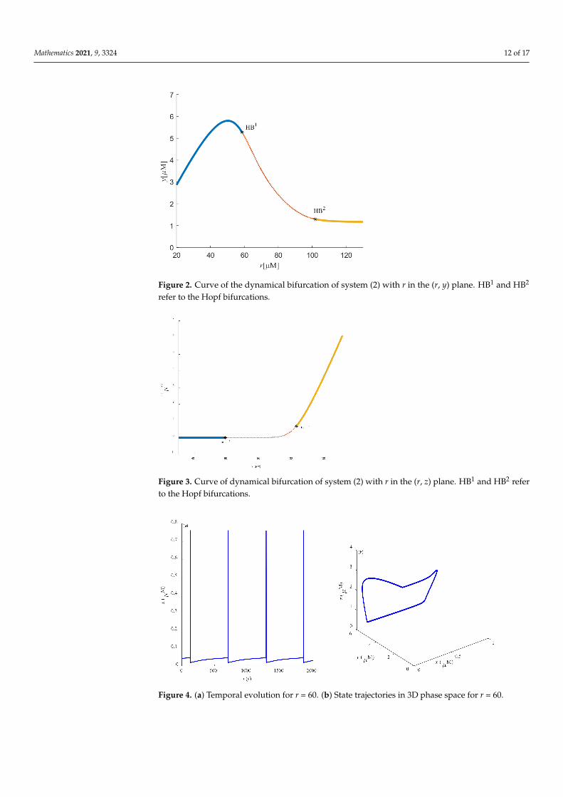
When the limit cycles pass through TR, the stability of the system limit cycles trans-forms further, and unstable limit cycles of the system turn into stable limit cycles. Torusbifurcation (TR) is a way to cause chaos in the system and is shown in the followingimages. Figures 2 and 3 represent the bifurcation diagram in the (r, y) and (r, z) planes,respectively. One can easily see that two Hopf bifurcation points appeared due to thevariation in parameter r.

Some dynamic behaviors of system (2) are schematically presented in Figures 4–10.Figures 4a–10a represent the temporal evolution for different values of parameter r.Figures 4b–10b correspond to different state trajectories in 3D phase space by varyingdifferent values of r. Among these, Figures 4–6, 8 and 9 represent the regular Ca2+ oscil-lations. Illustrations of chaos can be observed in Figures 7 and 10. These phenomena areabundant and need further study.

Mathematics 2021, 9, 3324 12 of 17

Figure 2. Curve of the dynamical bifurcation of system (2) with r in the (r, y) plane. HB1 and HB2

refer to the Hopf bifurcations.

Figure 3. Curve of dynamical bifurcation of system (2) with r in the (r, z) plane. HB1 and HB2 referto the Hopf bifurcations.

Figure 4. (a) Temporal evolution for r = 60. (b) State trajectories in 3D phase space for r = 60.

Mathematics 2021, 9, 3324 13 of 17

Figure 5. (a) Temporal evolution for r = 70. (b) State trajectories in 3D phase space for r = 70.

Figure 6. (a) Temporal evolution for r = 86. (b) State trajectories in 3D phase space for r = 86.

Figure 7. (a) Temporal evolution for r = 96. (b) State trajectories in 3D phase space for r = 96.

Mathematics 2021, 9, 3324 14 of 17

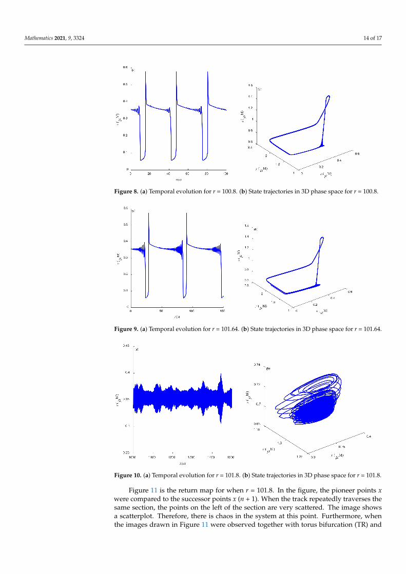
Figure 8. (a) Temporal evolution for r = 100.8. (b) State trajectories in 3D phase space for r = 100.8.

Figure 9. (a) Temporal evolution for r = 101.64. (b) State trajectories in 3D phase space for r = 101.64.

Figure 10. (a) Temporal evolution for r = 101.8. (b) State trajectories in 3D phase space for r = 101.8.

Figure 11 is the return map for when r = 101.8. In the figure, the pioneer points xwere compared to the successor points x (n + 1). When the track repeatedly traverses thesame section, the points on the left of the section are very scattered. The image showsa scatterplot. Therefore, there is chaos in the system at this point. Furthermore, whenthe images drawn in Figure 11 were observed together with torus bifurcation (TR) and

Mathematics 2021, 9, 3324 15 of 17

period doubling bifurcation (PD) in Figure 1 and the sequence diagram of time and phasediagram in Figure 10, we can see that the characteristics of system (2) displayed in theseimages were consistent and chaos was found in all of these diagrams, further validatingthe availability of the method.

Figure 11. Return map of Cacyt with r = 101.8.

Figure 12 investigates the Lyapunov exponential spectrum of system (2). Lyapunovexponent is a description of the stability of a dynamic system. When the Lyapunovexponent is greater than zero, it means chaos occurs in the system. For n-dimensionalcontinuous dynamical systems

.x = g (x), the system forms an n-dimensional sphere with x0

as the center and ‖δ x(x0,0) ‖ as the radius when t = 0. With the evolution of time, the spheredeforms into an n-dimensional ellipsoid at time t. Assume that the length of the half-axis inthe direction of the ith-axis of the ellipsoid is ‖δ xi (x0, t) ‖, then the ith-Lyapunov exponentof the system is

λi = limt→∞

1t

ln‖ δxi(x0, t) ‖‖ δx(x0, 0) ‖ .

Figure 12. Lyapunov index of system (2) with parameter r.

Solving the formula will give the Lyapunov exponent. In Figure 12, the yellow curvesrepresent LE1, the green curves represent LE2, and the blue curves represent LE3. The

Mathematics 2021, 9, 3324 16 of 17

Lyapunov exponent was more than 0 within a certain parameter range, indicating thepresence of chaos in system (2). For example, when r = 101.8, the corresponding Lyapunovexponents were LE1 = 0.1378, LE2 = −0.4361, and LE3 = −27.6405, respectively. LE1 > 0,so the system was in chaos at this point, which is consistent with Figure 1, Figure 10, andFigure 11.

5. Summary

In this study, the stability and bifurcation phenomena of a 3D Ca2+ oscillation modelwere investigated theoretically and simulated numerically. Oscillations of Ca2+ in the cy-tosol, endoplasmic reticulum, and mitochondria were studied using the total concentrationof Ca2+ in the cytosol, mitochondria, and endoplasmic reticulum as the bifurcation parame-ter. Two Hopf bifurcation points were obtained after varying the value of the parameter forinvestigation. There was a stable periodic solution near the supercritical Hopf bifurcationpoint. The Hopf bifurcation point was the source of oscillation.

After the theoretical analysis of the system, the correctness of the theoretical resultswas verified by the numerical method. During the numerical simulation, there were someinteresting oscillations. In addition to the usual simple oscillations, there were also someCa2+ oscillations of bursting. The peak values and periods of oscillations of differentbursting were also different, which may be related to bifurcation. Such findings providedideas for further research. Moreover, by exploring the bifurcation diagram, the Hopfbifurcation case calculated in this study well matched that of the image. Moreover, therewere also limit cycle LP and TR points. Where the system occurred, there was chaos at TR.This provided further insights into the dynamic behavior between the two points wherethe Hopf bifurcation occurs. In general, the total Ca2+ concentration greatly influences theformation and characteristics of Ca2+ oscillations in cells.

Some of the special phenomena found above need to be explored in more detail.Future works should select different models, explore different models, and conduct in-depth research. In addition, in many intracellular dynamic models, time delay has a certaineffect on the dynamic behavior of cells. However, the model established in this study didnot consider the effect of time delay. Therefore, in future works, the study of cell modelswith time delay is also worth considering.

Author Contributions: Conceptualization, Q.J.; methodology, X.Q.; software, X.Q.; validation, Q.J.;formal analysis, Q.J.; investigation, Q.J. and X.Q.; resources, Q.J. and X.Q.; data curation, X.Q.;writing—original draft preparation, X.Q.; writing—review and editing, Q.J. and X.Q.; visualization,X.Q.; supervision, Q.J.; project administration, Q.J.; funding acquisition, Q.J. All authors have readand agreed to the published version of the manuscript.

Funding: This work was supported by the Natural Science Foundation of China under GrantNos. 12062004, 11872084 and the Guangxi Natural Science Foundation under Grant No. GXNSFAA297240.

Institutional Review Board Statement: Not applicable.

Informed Consent Statement: Not applicable.

Data Availability Statement: All the data utilized in this article have been included, and the sourcesfrom where they were adopted were cited accordingly.

Conflicts of Interest: The authors declare no conflict of interest.

References1. Jaiswal, J.K. Calcium—How and why? J. Biosci. 2001, 26, 357–363. [CrossRef]2. Clapham, D.E. Calcium signaling. Cell 2007, 131, 1047–1058. [CrossRef] [PubMed]3. Leake, I. Microglial calcium activity in ischaemic brain injury. Nat. Rev. Neurol. 2021, 17, 2. [CrossRef]4. Bootman, M.D.; Collins, T.J.; Peppiatt, C.M.; Prothero, L.S.; Mackenzie, L.; Smet, P.D.; Travers, M.; Tovey, S.C.; Seo, J.T.;

Berridge, M.J.; et al. Calcium signalling—An overview. In Seminars in Cell & Developmental Biology; Academic Press: Cambridge,MA, USA, 2001; Volume 12, pp. 3–10.

5. Toyoshima, C.; Nomura, H. Structural changes in the calcium pump accompanying the dissociation of calcium. Nature 2002, 418,605–611. [CrossRef] [PubMed]

Mathematics 2021, 9, 3324 17 of 17

6. McAinsh, M.R.; Pittman, J.K. Shaping the calcium signature. New Phytol. 2009, 181, 275–294. [CrossRef]7. Blum, I.D.; Keles, M.F.; Baz, E.-S.; Han, E.; Park, K.; Luu, S.; Issa, H.; Brown, M.; Ho, M.C.W.; Tabuchi, M.; et al. Astroglial calcium

signaling encodes sleep need in Drosophila. Curr. Biol. 2021, 31, 150–162.e7. [CrossRef] [PubMed]8. Novikova, I.N.; Manole, A.; Zherebtsov, E.A.; Stavtsev, D.D.; Vukolova, M.N.; Dunaev, A.V.; Angelova, P.R.; Abramov, A.Y.

Adrenaline induces calcium signal in astrocytes and vasoconstriction via activation of monoamine oxidase. Free Radic. Biol. Med.2020, 159, 15–22. [CrossRef] [PubMed]

9. Lewis, K.J.; Frikha-Benayed, D.; Louie, J.; Stephen, S.; Spray, D.C.; Thi, M.M.; Seref-Ferlengez, Z.; Majeska, R.J.; Weinbaum, S.;Schaffler, M.B. Osteocyte calcium signals encode strain magnitude and loading frequency in vivo. Proc. Natl. Acad. Sci. USA 2017,114, 11775–11780. [CrossRef]

10. Siddiqui, M.H.; Al-Whaibi, M.H.; Basalah, M.O. Interactive effect of calcium and gibberellin on nickel tolerance in relation toantioxidant systems in Triticum aestivum L. Protoplasma 2011, 248, 503–511. [CrossRef] [PubMed]

11. Lautner, S.; Fromm, J. Calcium-dependent physiological processes in trees. Plant Biol. 2010, 12, 268–274. [CrossRef]12. Ahmad, P.; Sarwat, M.; Bhat, N.A.; Wani, M.R.; Kazi, A.G.; Tran, L.-S.P. Alleviation of cadmium toxicity in Brassica juncea L.

(Czern. & Coss.) by calcium application involves various physiological and biochemical strategies. PLoS ONE 2015, 10, e0114571.13. Shi, J.Q.; Wu, Z.X.; Song, L.R. Physiological and molecular responses to calcium supplementation in Microcystis aeruginosa

(Cyanobacteria). N. Z. J. Mar. Freshw. Res. 2013, 47, 51–61. [CrossRef]14. Endo, M. Calcium-induced calcium release in skeletal muscle. Physiol. Rev. 2009, 89, 1153–1176. [CrossRef] [PubMed]15. Carter, A.G.; Vogt, K.E.; Foster, K.A.; Regehr, W.G. Assessing the role of calcium-induced calcium release in short-term presynaptic

plasticity at excitatory central synapses. J. Neurosci. 2002, 22, 21–28. [CrossRef]16. Stern, M.D.; Cheng, H. Putting out the fire: What terminates calcium-induced calcium release in cardiac muscle. Cell Calcium

2004, 35, 591–601. [CrossRef]17. Wood, C.D.; Darszon, A.; Whitaker, M. Speract induces calcium oscillations in the sperm tail. J. Cell Biol. 2003, 161, 89–101.

[CrossRef] [PubMed]18. Wood, A.; Wing, M.G.; Benham, C.D. Specific induction of intracellular calcium oscillations by complement membrane attack on

oligodendroglia. J. Neurosci. 1993, 13, 3319–3332. [CrossRef] [PubMed]19. Borghans, J.A.M.; Dupont, G.; Goldbeter, A. Complex intracellular calcium oscillations A theoretical exploration of possible

mechanisms. Biophys. Chem. 1997, 66, 25–41. [CrossRef]20. Dupont, G.; Houart, G.; De Koninck, P. Sensitivity of CaM kinase II to the frequency of Ca2+ oscillations: A simple model. Cell

Calcium 2003, 34, 485–497. [CrossRef]21. Chay, T.R. Electrical bursting and luminal calcium oscillation in excitable cell models. Biol. Cybern. 1996, 75, 419–431. [CrossRef]22. Perc, M.; Marhl, M. Different types of bursting calcium oscillations in non-excitable cells. Chaos Solitons Fractals 2003, 18, 759–773.

[CrossRef]23. Shen, P.; Larter, R. Chaos in intracellular Ca2+ oscillations in a new model for non-excitable cells. Cell Calcium 1995, 17, 225–232.

[CrossRef]24. Marhl, M.; Haberichter, T.; Brumen, M.; Heinrich, R. Complex calcium oscillations and the role of mitochondria and cytosolic

proteins. BioSystems 2000, 57, 75–86. [CrossRef]25. Gellerich, F.N.; Gizatullina, Z.; Trumbeckaite, S.; Nguyen, H.P.; Pallaas, T.; Arandarcikaite, O.; Vielhaber, S.; Seppet, E.; Striggow, F.

The regulation of OXPHOS by extramitochondrial calcium. Biochim. Biophys. Acta (BBA)-Bioenerg. 2010, 1797, 1018–1027.[CrossRef]

26. Grubelnik, V.; Larsen, A.Z.; Kummer, U.; Olsen, L.F.; Marhl, M. Mitochondria regulate the amplitude of simple and complexcalcium oscillations. Biophys. Chem. 2001, 94, 59–74. [CrossRef]

27. Carr, J. Applications of Centre Manifold Theory; Springer Science & Business Media: Berlin/Heidelberg, Germany, 2012.28. Erhardt, A.H. Bifurcation analysis of a certain Hodgkin-Huxley model depending on multiple bifurcation parameters. Mathematics

2018, 6, 103. [CrossRef]29. Sun, M.; Li, Y.; Yao, W. A Dynamic Model of Cytosolic Calcium Concentration Oscillations in Mast Cells. Mathematics 2021,

9, 2322. [CrossRef]30. Zuo, H.; Ye, M. Bifurcation and Numerical Simulations of Ca2+ Oscillatory Behavior in Astrocytes. Front. Phys. 2020, 8, 258.

[CrossRef]31. Etter, D.M.; Kuncicky, D.C.; Hull, D.W. Introduction to MATLAB; Prentice Hall: Hoboken, NJ, USA, 2002.32. Venkataraman, P. Applied Optimization with MATLAB Programming; John Wiley & Sons: Hoboken, NJ, USA, 2009.