Bifurcation of a Coastal Current at an Escarpment

MAY 1999 969C A R N E V A L E E T A L .

q 1999 American Meteorological Society

Bifurcation of a Coastal Current at an Escarpment

GEORGE F. CARNEVALE

Scripps Institution of Oceanography, University of California, San Diego, La Jolla, California

STEFAN G. LLEWELLYN SMITH

Department of Applied Mathematics and Theoretical Physics, University of Cambridge, Cambridge, United Kingdom

FULVIO CRISCIANI AND ROBERTO PURINI

Istituto Talassografico-CNR, Trieste, Italy

ROBERTA SERRAVALL

Department of Mechanics and Aeronautics, University of Rome, La Sapienza, Rome, Italy

(Manuscript received 28 July 1997, in final form 16 June 1998)

ABSTRACT

The evolution of a coastal current as it encounters an escarpment depends strongly on whether the geometryof the coast and escarpment is right or left ‘‘handed,’’ independent of the direction of the coastal current.Handedness is defined such that right-handed means that when looking across the escarpment from the deep tothe shallow side, the coast is found on the right. The essential aspects of the difference in behavior of the currentin the two geometries are captured by a simple quasigeostrophic model of coastal flow over a step. An exactanalytic solution to the nonlinear stationary problem is obtained. This solution shows that, when a coastal currentcrosses an escarpment in the left-handed geometry, the speed of the current will increase independent of whetherthe flow is from shallow to deep or from deep to shallow. For the right-handed geometry, the speed of thecurrent decreases, also independent of the direction of the coastal flow. In the left (right)-handed geometry,there is associated to the coastal flow an inshore (offshore) current along the escarpment. These results areexplained in terms of linear wave theory and vortex dynamics. Numerical simulations are used to examine theevolution of the flow from the initial encounter to the establishment of a stationary flow. The relevance of thisresearch is discussed in light of recent results from laboratory experiments and oceanic observations.

1. Introduction

The presence of an escarpment, or step, may force acoastal current to bifurcate with one branch followingthe topographic contours of the step. As examples ofthis we can mention the Bering slope current (Kinderet al. 1986), the flow across the Adriatic Sea at theJabuka Pit (Poulain, manuscript submitted to J. Mar.Syst.), flow along the Iceland–Faeroe Ridge (Hansen andMeincke 1979), and the Kuroshio as it follows the con-tinental slope northeast of Taiwan (Hsueh et al. 1992;Stern and Austin 1995). In the ocean, many competingeffects may tend to obscure this phenomenon. Coastlineirregularity, complicated bottom topography, fluctua-

Corresponding author address: Dr. George F. Carnevale, ScrippsInstitution of Oceanography, University of California, La Jolla, CA92093-0225.E-mail: [email protected]

tions in the wind, baroclinic instabilities, and other ef-fects combine to make coastal current flow systems verycomplicated. Recent laboratory investigations havemodeled the bifurcation with homogeneous flow over asimple step (Spitz and Nof 1991; Stern and Austin1995). In these experiments, a wall jet is initiated fromrest and then propagates along the wall of the tank be-fore encountering a topographic step extending awayfrom the wall. Even these highly simplified model flowspresent some interesting surprises. For example, insteadof the expected simple bifurcation of the wall currentat the step, Stern and Austin (1995) found that the cur-rent was partially reflected at the step back toward thesource, with part continuing to follow the wall but withno flow along the slope. Spitz and Nof (1991) gaveexamples of simple coastal current bifurcations but insome cases observed strong eddy activity in the slopecurrent. In what follows, we will present results of an-alytical and numerical investigations based on the qua-

970 VOLUME 29J O U R N A L O F P H Y S I C A L O C E A N O G R A P H Y

FIG. 1. Schematic of the flow over a step problem in the (a) left-handed and (b) right-handed geometries. The coastline is indicatedby the solid lines. The open or inlet boundaries are indicated bydashed lines. The transition from deep to shallow fluid is indicatedby the gray region where we assume a smooth slope.

sigeostrophic model that, we hope, will elucidate var-ious aspects of this interesting problem.

The essential features of this problem are the presenceof the coast, the step, and the background rotation. Wewill assume a finite background rotation rate of the sys-tem in a counterclockwise sense (Northern Hemi-sphere). There are two basic configurations of interest.The geometry of these is shown in plan form in Fig. 1.The coastlines are indicated by the thick solid lines, andthe dashed lines indicate permeable or open boundaries.The topography changes from deep to shallow along thecoast, and the topographic slope is indicated by the areashaded gray. We call these geometries left-handed orright-handed depending on the orientation of the to-pography with the coast line. If we look in the directionof the gradient of the topography, that is from deep toshallow, and the coast is on the left (right), then werefer to the geometry as left-handed (right-handed) (inthe Northern Hemisphere). Another way to think of thisis to consider the triad of vectors formed by the normalto the coastline (pointing out from the ocean), the hor-izontal gradient of topography, and the ambient rotationvector in that order. We call the geometry right-handedif this triad is right-handed. We then imagine a currentflowing along the coast, coming initially from either thetop or the bottom of the diagrams, with its course in-tercepted by the topographic step. The presence of thestep may produce a bifurcation or even fully divert thecurrent. The dynamical problem also shows the possi-bility of the generation of eddies when the current firstencounters the slope. Due to the rotation, the flow inthe left-handed geometry (Fig. 1a) will be fundamen-tally different from that in the right-handed geometry(Fig. 1b).

One way to appreciate the difference between thedynamics of flows in the right- and left-handed geom-etries is to consider the propagation of topographicRossby waves in the system. We will consider the stepto be made of a smooth slope of finite extent from thedeep to shallow region. On this slope topographic Ross-by waves will exist that have a direct analogy to Rossby

waves on a b plane. The dispersion relation of Rossbywaves on the b plane in a flow under a rigid lid is

bkxv 5 2 , (1)k 2 2k 1 kx y

where the positive x direction corresponds to due east.Therefore, the group velocity is given by

b2 2c 5 (k 2 k , 2k k ). (2)g x y x y2 2 2(k 1 k )y x

Thus, waves that are relatively long in the x direction(i.e., |kx/ky| K 1) will have a westward component ofpropagation, while waves that are relatively short in thex direction (i.e., |kx/ky| k 1) will have an eastward com-ponent of propagation (cf. Pedlosky 1965). In quasi-geostrophic theory, the b effect is equivalent to the ef-fect of a bottom slope of magnitude f 0m/H0, where f 0

is the Coriolis parameter, m the slope of the bottom inthe y direction, and H0 the mean depth of the fluid.Confining the extent of the slope in the y direction willchange the dispersion relation somewhat (in particularthe ky values become discrete), but, nevertheless, thesimilarity with the dispersion relation (1) is sufficientto draw the same conclusion about propagation direc-tions. Thus considering Fig. 1, in both the left- and right-handed cases as drawn, the topographic waves long inx will propagate toward the left, that is, toward the coastin the left-handed geometry and away from the coastin the right-handed geometry. Thus a disturbance causedby the interaction of a coastal flow over the topographyshould be expected to propagate very differently in thetwo geometries. Although this is only a part of the pic-ture since the flows are nonlinear and flow structuresother than waves will be found to play an importantrole, this view of the wave dynamics provides an im-portant insight into the difference in the behavior of theflow in the two geometries.

The importance of the difference in the direction ofpropagation of the long topographic waves for the coast-al escarpment problem has been pointed out in severalprevious articles, particularly in regard to the shallow-water version of the problem (cf. Rhines 1969; Johnson1985; Gill et al. 1986; Willmott and Grimshaw 1991;Johnson and Davey 1990; Allen 1988, 1996; and Allenand Hsieh 1997). Many of the previous analytical stud-ies focused on linear wave propagation in shallow-watertheory. Although the propagation of topographic wavesis an important part of the evolution of the flow, non-linear effects can change the nature of the evolution andthe long-term state significantly compared to the linearpredictions. By using the quasigeostrophic model of thisproblem, we are able to present here a fully nonlinearsteady-state solution, which has not appeared previous-ly. This solution is very different from the correspond-ing solution obtained in linear shallow-water orquasigeostrophic theory as we will discuss below. In


addition, we will see how the transient evolution of theflow involves nonlinear coherent flow structures.

We begin, in the next section, by defining the stepproblem in the context of the quasigeostrophic modeland providing some analytic solutions for the steady-state case. Then in section 3 we will compare thesepredictions to the results from numerical simulations.The simulations are performed with a finite-differencemodel that follows the evolution of a coastal currentforced by inflow boundary conditions, from an initialstate of no motion. Finally, in the discussion section,we will attempt to provide some physical insight intothe differences for flow in the left-handed and right-handed geometries and also point out the connection tocertain oceanographic observations.

2. An analytic steady-state solution

The simplest model of rotating flow that captures theessential ingredients of the coastal step problem is thebarotropic quasigeostrophic model. The governingequation, which expresses the conservation of potentialvorticity, may be written as

D(v 1 h) 5 0, (3)

Dt

or more explicitly as

]v1 J(c, v 1 h) 5 0, (4)

]t

where c is the streamfunction, v 5 ¹2c is the relativevorticity, and J is the Jacobian. The topographic termh is given by

DHh 5 2 f , (5)

H0

where H is the height of fluid column above the topog-raphy with the mean given by H0. Thus,

hH 5 H 1 DH 5 H 1 2 . (6)0 01 2f

The sign convention for h is such that it is positivepositive over hills and negative over valleys.

The appropriate form of the equation for steady flowis then

J(c, ¹2c 1 h) 5 0. (7)

The solution to this equation is

¹2c 1 h 5 F(c) (8)

for some function F, which simply means that the con-tours of potential vorticity, ¹2c 1 h, coincide with thecontours of the streamfunction. The function F is, tosome degree, determined by the boundary conditions,as will be discussed below.

The streamfunction may be decomposed into an un-

perturbed coastal current C(x) and a topographic re-sponse w(x, y), where we are using the traditional co-ordinate system with x running from left to right and yfrom bottom to top in the figures. We will begin byfinding an analytic solution for the case where the coast-al current is defined by a boundary condition at y 52`, where we will assume w 5 0. Alternate formula-tions with the boundary conditions at y 5 1` will bediscussed later. Only the gradient of the topography isimportant for (3) and not the absolute depth, and it willbe convenient to take h(x, 2`) 5 0. Although it is notthe only possibility, consider first the case in which Fis defined to be the same function everywhere. Notingthat there is no explicit dependence on position in (8),we consider it in the limit of y → 2`. There we have

c [ C 1 w → C (9)2 2¹ c 1 h → ¹ C. (10)

Thus

Cxx(x) 5 F(C(x)). (11)

The form of the unperturbed coastal current C(x) thendetermines the function F. Also, we see at this pointthat, if we had set h(x, 2`) to a constant value otherthan zero, this would have just altered the definition ofF by a constant value.

The profile of coastal current that renders our problemmost amenable to analysis is exponential. Accordingly,we take

C(x) 5 C0e2lx. (12)

We will refer to l21 as the width of the current. Thisprofile is also convenient because, having no inflectionpoint in the vorticity, it is barotropically stable. Thevelocity V 5 2lC and vorticity v 5 l2C of the coastaljet are greatest in magnitude on the coast. This profileis only possible when the coast is modeled as a slipboundary. Such boundary conditions are often usedwhen the details of the coastal region cannot be resolvedand when it is reasonable to model the large-scale mo-tions as a flow slipping past the coast on a buffer zonethat effects that actual transition of the flow to the no-slip shore (cf. Pond and Pickard 1978; Pedlosky 1996).

The exponential profile implies that F is linear. FromEq. (11) we have

F(C) 5 l2C. (13)

Using this function F in the governing equation (8) forthe topographic response leads to

(¹2 2 l2)w 5 2h. (14)

Thus, we arrive at an inhomogeneous Helmholtz equa-tion for the response w. In addition to the vanishing ofw for y → 2`, we also demand that it vanish on thecoast (x 5 0) so that there is no flow through the coast.

It is worth emphasizing that the sum c 5 C 1 w isan exact solution of the fully nonlinear equation of mo-


FIG. 2. Contour plot of the topography-induced streamfunction wgiven by (18) and (22) for the particular form of topography givenin (23). The contour interval is 0.2|h0/l2|. The arrows indicate thedirection of the current represented by w. Gray shading representsthe region of the slope of width w. Here l21 5 0.5w.

tion (3). It is interesting that the topographic responsesatisfies a linear inhomogeneous equation. Hence, w isproportional to the topography, but can be of any am-plitude compared to the coastal jet.

The solution for w will be determined by a Greenfunction approach. The Green function for the Helm-holtz operator (¹2 2 l2) on an infinite plane is G(r, r9)5 2(1/2p)K0(|r 2 r9|), where r 5 (x, y) and K0 is themodified Bessel function of order 0. To meet the con-dition of no flow through the coastal boundary, one canadd to this free-space Green function another with itssingularity placed to the left of the coastline such thatthe combination vanishes when x 5 x9. Thus the half-plane Green function is

1G(r, r9) 5 2 [K (|r 2 r9|) 2 K (|r 2 r0|)], (15)0 02p

where r0 5 (2x9, y9). Then the formal solution to (14) is

w 5 2 dx9 dy9G(r, r9)h(y9), (16)EEwhere the minus sign arises since the forcing in (14) is2h. The form of the Green function used here makesit difficult to exploit the fact that h is independent of x.After performing the x9 integral in (16) and followinga tedious series of nonobvious transformations, a muchsimpler Green function with no dependence on x9 canbe obtained. Rather than pursue this route, we will pre-sent a much simpler derivation of the result.

To find a simpler representation of the Green function,we solve for the reduced Green function g(x, y 2 y9)directly by solving

(¹2 2 l2)g(x, y 2 y9) 5 d(y 2 y9), (17)

where d(y 2 y9) is the Dirac delta function (cf. Gel’fandand Shilov 1964). Once g is obtained, w will be ex-pressible as a one-dimensional integral:

`

w 5 2g∗h [ 2 g(x, y 2 y9)h(y9) dy9. (18)E2`

Note that we use an asterisk to represent convolution.To solve (17), we first Fourier transform in y, whichleads to

gxx 2 (l2 1 l2)g 5 1. (19)

The general solution to this equation is

1 2 2 1/2 2 2 1/22(l 1l ) x 1(l 1l ) xg 5 2 1 Ae 1 Be . (20)2 2l 1 l

Demanding that g remains bounded as x → ` and thatg(0, y 2 y9) 5 0, so that w will satisfy the appropriateboundary conditions, then leads to

2 2 1/22(l 1l ) xe 2 1g 5 , (21)

2 2[ ]l 1 l` 2ly |y |1 e

2 1/2g(x, y) 5 2 sin(lx[y 2 1] ) dy , (22)E 2pl y 2 11

The details of the calculation are presented in the ap-pendix. This approach was also taken by E. R. Johnson(1978, unpublished manuscript).

It is clear from (22) that the Green function for theproblem is symmetric in y, as might be expected. Inessence, the Green function does not contain informa-tion about the form of the topography. With this Greenfunction, the upstream boundary condition that we usedon the topography, h(x, 2`) 5 0, guarantees the van-ishing of w(x, 2`). This, of course, can be changed ifwe want the unperturbed current to flow in the oppositedirection, that is, if we have the inlet condition at y 51`. This change of boundary condition is simply ac-complished by adding a dynamically insignificant con-stant to h so that h(x, `) 5 0 and then we would havew(x, `) 5 0.

An example of the solution w(x, y) for the inlet con-ditions at y 5 2` is shown in Fig. 2. Here we havetaken a particular form of h given in terms of a stretchedcoordinate h by

h if h . 102 3h 5 h (3h 2 2h ) if 0 # h # 1 (23)0

0 if h , 0,

where h 5 (y 1 w/2)/w in which w is the width of the


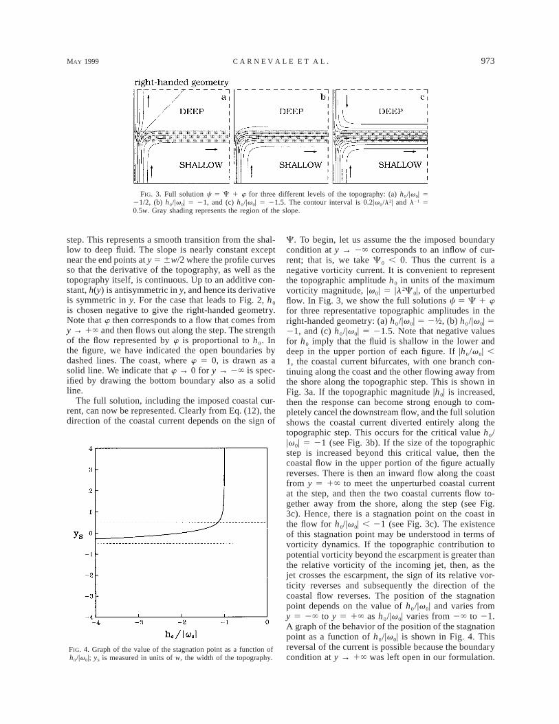
FIG. 3. Full solution c 5 C 1 w for three different levels of the topography: (a) h0/|v0| 521/2, (b) h0/|v0| 5 21, and (c) h0/|v0| 5 21.5. The contour interval is 0.2|v0/l2| and l21 50.5w. Gray shading represents the region of the slope.

FIG. 4. Graph of the value of the stagnation point as a function ofh0/|v0|; yS is measured in units of w, the width of the topography.

step. This represents a smooth transition from the shal-low to deep fluid. The slope is nearly constant exceptnear the end points at y 5 6w/2 where the profile curvesso that the derivative of the topography, as well as thetopography itself, is continuous. Up to an additive con-stant, h(y) is antisymmetric in y, and hence its derivativeis symmetric in y. For the case that leads to Fig. 2, h0

is chosen negative to give the right-handed geometry.Note that w then corresponds to a flow that comes fromy → 1` and then flows out along the step. The strengthof the flow represented by w is proportional to h0. Inthe figure, we have indicated the open boundaries bydashed lines. The coast, where w 5 0, is drawn as asolid line. We indicate that w → 0 for y → 2` is spec-ified by drawing the bottom boundary also as a solidline.

The full solution, including the imposed coastal cur-rent, can now be represented. Clearly from Eq. (12), thedirection of the coastal current depends on the sign of

C. To begin, let us assume the the imposed boundarycondition at y → 2` corresponds to an inflow of cur-rent; that is, we take C0 , 0. Thus the current is anegative vorticity current. It is convenient to representthe topographic amplitude h0 in units of the maximumvorticity magnitude, |v0| 5 |l2C0|, of the unperturbedflow. In Fig. 3, we show the full solutions c 5 C 1 wfor three representative topographic amplitudes in theright-handed geometry: (a) h0/|v0| 5 2½, (b) h0/|v0| 521, and (c) h0/|v0| 5 21.5. Note that negative valuesfor h0 imply that the fluid is shallow in the lower anddeep in the upper portion of each figure. If |h0/v0| ,1, the coastal current bifurcates, with one branch con-tinuing along the coast and the other flowing away fromthe shore along the topographic step. This is shown inFig. 3a. If the topographic magnitude |h0| is increased,then the response can become strong enough to com-pletely cancel the downstream flow, and the full solutionshows the coastal current diverted entirely along thetopographic step. This occurs for the critical value h0/|v0| 5 21 (see Fig. 3b). If the size of the topographicstep is increased beyond this critical value, then thecoastal flow in the upper portion of the figure actuallyreverses. There is then an inward flow along the coastfrom y 5 1` to meet the unperturbed coastal currentat the step, and then the two coastal currents flow to-gether away from the shore, along the step (see Fig.3c). Hence, there is a stagnation point on the coast inthe flow for h0/|v0| , 21 (see Fig. 3c). The existenceof this stagnation point may be understood in terms ofvorticity dynamics. If the topographic contribution topotential vorticity beyond the escarpment is greater thanthe relative vorticity of the incoming jet, then, as thejet crosses the escarpment, the sign of its relative vor-ticity reverses and subsequently the direction of thecoastal flow reverses. The position of the stagnationpoint depends on the value of h0/|v0| and varies fromy 5 2` to y 5 1` as h0/|v0| varies from 2` to 21.A graph of the behavior of the position of the stagnationpoint as a function of h0/|v0| is shown in Fig. 4. Thisreversal of the current is possible because the boundarycondition at y → 1` was left open in our formulation.


FIG. 5. Contour plot of the full solution c 5 C 1 w with outflowon the bottom boundary for the topography such that h0/|v0| 5 21/2. The contour interval is 0.1|v0/l2|. Gray shading represents theregion of the slope.

FIG. 6. Contour plot of the full solution c 5 C 1 w for the to-pography such that h0/|v0| 5 1/2. The contour interval is 0.1|v0/l2|.Gray shading represents the region of the slope.

By setting the relation F between streamfunction andpotential vorticity to be the same everywhere, we haveinduced a strong inflowing current from the downstreamboundary when h0 is sufficiently negative. If we wantto impose a ‘‘downstream’’ condition that does not allowsuch inflow, we would need to introduce different valuesof F in different regions as discussed below, and thenthe problem becomes analytically intractable.

The solutions discussed so far were constrained bythe requirement that we specify the coastal flow at y 52` as an inflow. If we relax this condition and changethe sign of C0, thus specifying an outflow at y 5 2`,then additional solutions are possible. For the right-handed geometry, the form of these solutions is alwaysas shown in Fig. 5, independent of the magnitude of h0.This is because the perturbation w (see Fig. 2) has aflow in the same direction as the unperturbed currentalong the coast. Thus we cannot reverse the directionof the coastal current by changing the magnitude of h0

in this case.Next we shall consider the solutions in the left-handed

geometry. The forms of these solutions can be obtaineddirectly from the solutions given above for the right-handed geometry by a simple symmetry transformation.From (7), we see that for every solution c with giventopography h, we have the corresponding solution de-fined by the transformation c(x, y) → 2c(x, y) and h(y)→ 2h(y). Thus, for example, this transformation appliedto the case shown in Fig. 5 for flow in the right-handedgeometry with outflow specified at y 5 2` producesthe result shown in Fig. 6 for flow in the left-handedgeometry with inflow specified at y 5 2`.

Similarly, all of the right-handed geometry solutionsshown in Fig. 3 have their counterparts in the left-hand-ed geometry as shown in Fig. 7. The solid line on thebottom of the diagrams now indicates the boundarywhere the outflow is the prescribed exponential func-tion.

The remarkable thing about the solutions for the left-handed geometry is that the flow along the step is alwaystoward the coast. The steady coastal current across thestep in the left-handed geometry does not bifurcate, butrather is joined by an inshore current flowing along thestep, which reinforces the coastal current—in the casein Figs. 7b,c the step current is the source for the entirecoastal current. Thus, as long as the relationship be-tween streamfunction and potential vorticity is set at thethe boundary at y → 2`, there is only one stationaryflow, and it has this feature of inflow along the step.

We can see how the handedness of the geometry de-termines the direction of the flow along the step in oursolution by examining the far field (x → `). The be-havior of (22) for large x may be found after makingthe change of variable s2 5 y 2 2 1. Then

` 2 1/22l(11s ) |y |1 sin(lxs) h∗ew 5 ds. (24)E 2 1/2pl s (1 1 s )0

Note that

sin(lxs)lim 5 pd(s), (25)

sx→`

where d( ) is the Dirac delta function (cf. Messiah 1961).Thus, in the limit x → `, we have


FIG. 7. Full solution c 5 C 1 w, with outflow specified at y → 2`, for three different levelsof the topography: (a) h0/|v0| 5 1/2, (b) h0/|v0| 5 1, and (c) h0/|v0| 5 1.5. The contour interval0.2|v0/l2|. Gray shading represents the region of the slope.

FIG. 8. Stationary streamfunction in the right-handed geometry for|h0/v0| 5 0.5 for (a) step-down configuration and (b) step-up config-uration. The contour interval is 0.1|h0/l2|. Gray shading representsthe position of the slope.

2l |y |h∗ew 5 , (26)

2l

where the factor of ½ arises from the fact that the in-tegral terminates at s 5 0. This is exactly the solutionto the one-dimensional problem,

wyy 2 l2w 1 h 5 0, (27)

which is what would be expected from Eq. (14) at largedistances x where the x dependence vanishes.

Since there is no x variation in the far field result(26), for large x the velocity is directed only along thestep and is given by

2l |y |eu 5 2 ∗h9(y). (28)

2l

The right-handed geometry (with the wall on the left)has h9(y) , 0, so the flow far from the coast will bedirected away from the shore. For the left-handed ge-ometry, h9(y) . 0, and the flow will be toward the coast.Furthermore, from Eq. (27), it follows that for large xand large |y| we have w 5 h/l2. Thus, the total massflux leaving the domain along the step is

1` h0u dy 5 2(w(1`) 2 w(2`)) 5 2 . (29)E 2l2`

Note that this is independent of the mass flux entering

the domain with the inlet coastal current. Any differencebetween the two is compensated by the flow throughthe top boundary (i.e., y 5 1`).

Up to this point, we have been displaying only so-lutions for the case with the unperturbed coastal flowspecified at y 5 2`. What happens if the unperturbedcoastal current is specified at y 5 1`? The result canbe deduced from the solutions given above and sym-metry considerations. Let us assume that the topogra-phy, save perhaps for an additive constant, is antisym-metric in y, which means that the gradient of the to-pography is symmetric in y. Consequently, if we havea solution to the stationary state equation (7) given byc 5 C(x) 1 w(x, y), then c 5 2C(x) 2 w(x, 2y) isalso a solution, as can be seen by substituting this formfor c in the Jacobian, J(c, ¹2c 1 h). Exploiting thesymmetry of ]h/]y and making the change of variablesy → 2y then shows that the Jacobian must vanish. Thus,for the given topography, the form of the streamfunc-tions will not change under coastal current reversal savefor this simple symmetry transformation. This is illus-trated for the right-handed geometry in Fig. 8. Note thatin Fig. 8b the inflow boundary condition is specified onthe top boundary as indicated by the solid line. In bothcases shown, with the coastal flow encountering eithera step up or step down, the flow along the step is directedoffshore. Similarly, if we consider the left-handed ge-ometry, we find that the topographic current is towardthe coast irrespective of whether the coastal flow en-counters a step up or step down. It is the handednessof the geometry that determines the direction of thecurrent on the step and not the direction of the coastalcurrent.

We must end this section with a note of caution. Thesolution obtained here is not unique. Even assuming thespecific exponential inflow boundary condition as wedid, there is still an element of ambiguity introduced bythe lack of explicit boundary conditions on the down-stream and offshore boundaries. For example, we couldspecify the downstream boundary with an inflow ve-locity profile rather different from that found in ouranalytic solution. This would necessitate introducing an-


other form for F in the region of that boundary. We canin general imagine the function F specified differentlyin different regions of the flow. The values of F in eachregion would be determined by the relation betweenstreamfunction and potential vorticity on the adjacentexternal boundaries through which streamlines pass.Boundaries between different regions of F in the interiorof the flow are acceptable as long as those boundariesare streamlines. In fact, wholly interior regions with anarbitrary specification of F would also be possible aslong as there is no exchange of fluid with such a regionand the surrounding flow. The appropriate choice ofboundary conditions will depend on the specific natureof the problem under consideration. Here the flows onthe originally unspecified boundaries are determined byour demand that F be the same function everywhere.Thus, we must expect that the analytic solution will bevalid everywhere only when all of the streamlines inthe flow intersect the boundary where we have specifiedthe relation between streamfunction and potential vor-ticity (i.e., in the cases for which |h0/v0| , 1).

3. Numerical simulations

We have performed a series of numerical simulationsof the quasigeostrophic flow over a step. The geometryfor the numerical simulations is the same as that con-sidered above with the step profile given by (23). Hereour main interest is to gain insight into the dynamicsof the interaction of the coastal flow with the step. Theboundary conditions, as described below, are designedto focus attention on the dynamics of the interactionrather than to reproduce our analytic solution.

We begin the simulations from a state of no motionand introduce a coastal flow at one boundary. The flowthrough this inlet boundary is smoothly increased duringa period of two advective time units to the steady stateexponential velocity profile given in (12). We define theadvective time unit as 1/v0, or equivalently 1/(lV0),where V0 is the maximum velocity and l21 is the widthof the coastal unperturbed steady current. The inletboundary is taken sufficiently far from the topographyso as to minimize the effects of the finite size compu-tational domain.

Since we are mainly concerned with understandingthe results of the interaction of our coastal current andthe topography, we have used a radiation boundary con-dition on the open ocean and the downstream bound-aries. This is the choice that best represents the dynam-ics of the interaction between the approaching coastalcurrent and the escarpment on a semi-infinite domain.These boundary conditions will minimize the effects ofthe geometry of the computational boundaries other thanthat of the coast. However, the downstream and offshoreboundary conditions of the simulation differ from theanalytical steady-state solution in cases that requirespecification of inflow on offshore and downstreamboundaries because the flow on the radiation boundaries

can only evolve due to the influence of the vorticityfield within the computational domain. For the radiationcondition we use the Orlanski (1976) algorithm. In thismethod the boundary conditions for c and v arechanged each time step according to an estimate of therate of change of these quantities near the boundaryfrom previous time steps.

For the coastal boundary, we use a slip boundarycondition. For the streamfunction this simply means thatwe impose that c is a fixed constant on the wall, whichimplies no normal flow. The presence of Laplacian dif-fusion in our code raises a complication, however. Un-fortunately this diffusion cannot be set equal to zero inthis finite difference code without losing numerical sta-bility. With finite viscosity, we will also need to specifythe vorticity at the slip wall. The typical stress-freeboundary conditions on a straight boundary would re-quire that we set v 5 0. This, however, is inappropriatefor the present problem for two reasons. One is that thecoastal current that we want to model has maximumvorticity at the wall. The second, and perhaps moreimportant reason, is that as a fluid particle moving alongthe boundary encounters the topography its relative vor-ticity must change by vortex stretching. Similar dilem-mas have been faced in other applications as discussedby Roache (1972). The remedy that seems best for thepresent problem is to take the values of v on the wallto be identical to those just off the wall. Thus as thenearby particles adjust to changes in topography, thesame adjustment is forced at the wall. Thus, we haveimposed ]v/]n 5 0 at the wall where n is the coordinatein the direction normal to the wall. This boundary con-dition is sometimes referred to as ‘‘superslip’’ (cf. Ped-losky 1996).

The time stepping in these simulations is Runge–Kut-ta third order, which is optimal for efficient memoryusage (Rai and Moin 1991) and permits a fairly largetime step. The size of the time step is adjusted aftereach step according to the conditions of the CFL cri-terion (cf. Peyret and Taylor 1983) permitting high ef-ficiency.

As a first example, we consider the case of the right-handed geometry with an inlet condition such that h0/|v0| 5 20.5. In this case, the analytic theory predictsthat in the steady state the coastal current bifurcates withone branch following the coast and the other flowingoutward along the step. We began by simulating theevolution of the flow from rest until a stationary statewas reached at Reynolds number 750 defined by Re 5V0l21/n. This stationary state was close to the theoret-ical prediction, but the results were improved somewhatby continuing the evolution at Reynolds number 2500.The result for this high Reynolds number, long-termevolution is shown in Fig. 9. In panel (a) we show thestreamfunction from the simulation (solid contours) su-perimposed on the theoretical streamfunction (dottedcontours). The resulting match is nearly perfect. Theone contour that does not match well is in a region of


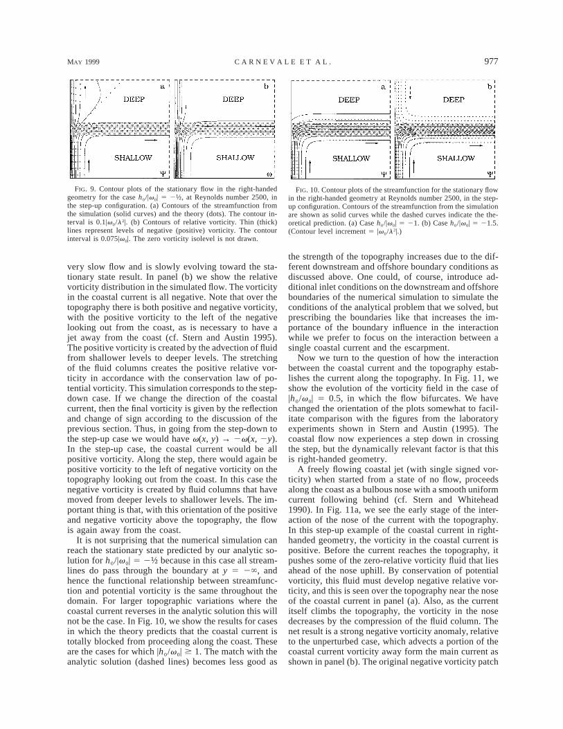
FIG. 9. Contour plots of the stationary flow in the right-handedgeometry for the case h0/|v0| 5 2½, at Reynolds number 2500, inthe step-up configuration. (a) Contours of the streamfunction fromthe simulation (solid curves) and the theory (dots). The contour in-terval is 0.1|v0/l2|. (b) Contours of relative vorticity. Thin (thick)lines represent levels of negative (positive) vorticity. The contourinterval is 0.075|v0|. The zero vorticity isolevel is not drawn.

FIG. 10. Contour plots of the streamfunction for the stationary flowin the right-handed geometry at Reynolds number 2500, in the step-up configuration. Contours of the streamfunction from the simulationare shown as solid curves while the dashed curves indicate the the-oretical prediction. (a) Case h0/|v0| 5 21. (b) Case h0/|v0| 5 21.5.(Contour level increment 5 |v0/l2|.)

very slow flow and is slowly evolving toward the sta-tionary state result. In panel (b) we show the relativevorticity distribution in the simulated flow. The vorticityin the coastal current is all negative. Note that over thetopography there is both positive and negative vorticity,with the positive vorticity to the left of the negativelooking out from the coast, as is necessary to have ajet away from the coast (cf. Stern and Austin 1995).The positive vorticity is created by the advection of fluidfrom shallower levels to deeper levels. The stretchingof the fluid columns creates the positive relative vor-ticity in accordance with the conservation law of po-tential vorticity. This simulation corresponds to the step-down case. If we change the direction of the coastalcurrent, then the final vorticity is given by the reflectionand change of sign according to the discussion of theprevious section. Thus, in going from the step-down tothe step-up case we would have v(x, y) → 2v(x, 2y).In the step-up case, the coastal current would be allpositive vorticity. Along the step, there would again bepositive vorticity to the left of negative vorticity on thetopography looking out from the coast. In this case thenegative vorticity is created by fluid columns that havemoved from deeper levels to shallower levels. The im-portant thing is that, with this orientation of the positiveand negative vorticity above the topography, the flowis again away from the coast.

It is not surprising that the numerical simulation canreach the stationary state predicted by our analytic so-lution for h0/|v0| 5 2½ because in this case all stream-lines do pass through the boundary at y 5 2`, andhence the functional relationship between streamfunc-tion and potential vorticity is the same throughout thedomain. For larger topographic variations where thecoastal current reverses in the analytic solution this willnot be the case. In Fig. 10, we show the results for casesin which the theory predicts that the coastal current istotally blocked from proceeding along the coast. Theseare the cases for which |h0/v0| $ 1. The match with theanalytic solution (dashed lines) becomes less good as

the strength of the topography increases due to the dif-ferent downstream and offshore boundary conditions asdiscussed above. One could, of course, introduce ad-ditional inlet conditions on the downstream and offshoreboundaries of the numerical simulation to simulate theconditions of the analytical problem that we solved, butprescribing the boundaries like that increases the im-portance of the boundary influence in the interactionwhile we prefer to focus on the interaction between asingle coastal current and the escarpment.

Now we turn to the question of how the interactionbetween the coastal current and the topography estab-lishes the current along the topography. In Fig. 11, weshow the evolution of the vorticity field in the case of|h0/v0| 5 0.5, in which the flow bifurcates. We havechanged the orientation of the plots somewhat to facil-itate comparison with the figures from the laboratoryexperiments shown in Stern and Austin (1995). Thecoastal flow now experiences a step down in crossingthe step, but the dynamically relevant factor is that thisis right-handed geometry.

A freely flowing coastal jet (with single signed vor-ticity) when started from a state of no flow, proceedsalong the coast as a bulbous nose with a smooth uniformcurrent following behind (cf. Stern and Whitehead1990). In Fig. 11a, we see the early stage of the inter-action of the nose of the current with the topography.In this step-up example of the coastal current in right-handed geometry, the vorticity in the coastal current ispositive. Before the current reaches the topography, itpushes some of the zero-relative vorticity fluid that liesahead of the nose uphill. By conservation of potentialvorticity, this fluid must develop negative relative vor-ticity, and this is seen over the topography near the noseof the coastal current in panel (a). Also, as the currentitself climbs the topography, the vorticity in the nosedecreases by the compression of the fluid column. Thenet result is a strong negative vorticity anomaly, relativeto the unperturbed case, which advects a portion of thecoastal current vorticity away form the main current asshown in panel (b). The original negative vorticity patch


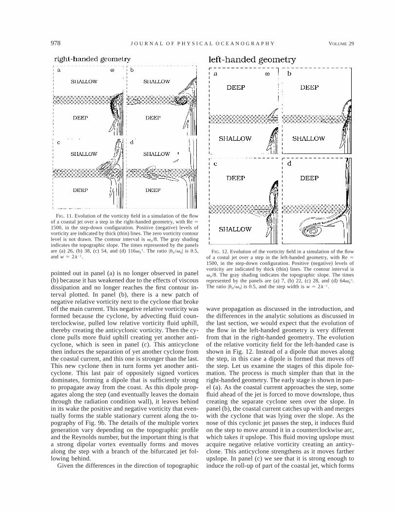
FIG. 11. Evolution of the vorticity field in a simulation of the flowof a coastal jet over a step in the right-handed geometry, with Re 51500, in the step-down configuration. Positive (negative) levels ofvorticity are indicated by thick (thin) lines. The zero vorticity contourlevel is not drawn. The contour interval is v0/8. The gray shadingindicates the topographic slope. The times represented by the panelsare (a) 26, (b) 38, (c) 54, and (d) . The ratio |h0/v0| is 0.5,21116v0

and w 5 2l21.FIG. 12. Evolution of the vorticity field in a simulation of the flow

of a costal jet over a step in the left-handed geometry, with Re 51500, in the step-down configuration. Positive (negative) levels ofvorticity are indicated by thick (thin) lines. The contour interval isv0/8. The gray shading indicates the topographic slope. The timesrepresented by the panels are (a) 7, (b) 22, (c) 28, and (d) .2164v0

The ratio |h0/v0| is 0.5, and the step width is w 5 2l21.

pointed out in panel (a) is no longer observed in panel(b) because it has weakened due to the effects of viscousdissipation and no longer reaches the first contour in-terval plotted. In panel (b), there is a new patch ofnegative relative vorticity next to the cyclone that brokeoff the main current. This negative relative vorticity wasformed because the cyclone, by advecting fluid coun-terclockwise, pulled low relative vorticity fluid uphill,thereby creating the anticyclonic vorticity. Then the cy-clone pulls more fluid uphill creating yet another anti-cyclone, which is seen in panel (c). This anticyclonethen induces the separation of yet another cyclone fromthe coastal current, and this one is stronger than the last.This new cyclone then in turn forms yet another anti-cyclone. This last pair of oppositely signed vorticesdominates, forming a dipole that is sufficiently strongto propagate away from the coast. As this dipole prop-agates along the step (and eventually leaves the domainthrough the radiation condition wall), it leaves behindin its wake the positive and negative vorticity that even-tually forms the stable stationary current along the to-pography of Fig. 9b. The details of the multiple vortexgeneration vary depending on the topographic profileand the Reynolds number, but the important thing is thata strong dipolar vortex eventually forms and movesalong the step with a branch of the bifurcated jet fol-lowing behind.

Given the differences in the direction of topographic

wave propagation as discussed in the introduction, andthe differences in the analytic solutions as discussed inthe last section, we would expect that the evolution ofthe flow in the left-handed geometry is very differentfrom that in the right-handed geometry. The evolutionof the relative vorticity field for the left-handed case isshown in Fig. 12. Instead of a dipole that moves alongthe step, in this case a dipole is formed that moves offthe step. Let us examine the stages of this dipole for-mation. The process is much simpler than that in theright-handed geometry. The early stage is shown in pan-el (a). As the coastal current approaches the step, somefluid ahead of the jet is forced to move downslope, thuscreating the separate cyclone seen over the slope. Inpanel (b), the coastal current catches up with and mergeswith the cyclone that was lying over the slope. As thenose of this cyclonic jet passes the step, it induces fluidon the step to move around it in a counterclockwise arc,which takes it upslope. This fluid moving upslope mustacquire negative relative vorticity creating an anticy-clone. This anticyclone strengthens as it moves fartherupslope. In panel (c) we see that it is strong enough toinduce the roll-up of part of the coastal jet, which forms


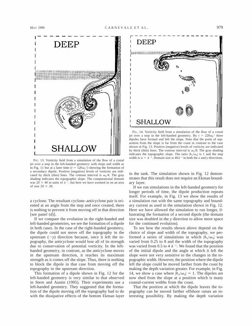
FIG. 13. Vorticity field from a simulation of the flow of a costaljet over a step in the left-handed geometry with slope and width asin Fig. 11 but at a later time (t 5 ) showing the formation of21120v0

a secondary dipole. Positive (negative) levels of vorticity are indi-cated by thick (thin) lines. The contour interval is v0/4. The grayshading indicates the topographic slope. The computational domainwas 20 3 40 in units of l21, but here we have zoomed in on an areaof size 20 3 28.

FIG. 14. Vorticity field from a simulation of the flow of a costaljet over a step in the left-handed geometry. By t 5 three21220v0

dipoles have formed and left the slope. Note that the point of sep-aration from the slope is far from the coast in contrast to the caseshown in Fig. 13. Positive (negative) levels of vorticity are indicatedby thick (thin) lines. The contour interval is v0/8. The gray shadingindicates the topographic slope. The ratio |h0/v0| is 1 and the stepwidth is w 5 l21. Domain size is 40l21 in both the x and y directions.

a cyclone. The resultant cyclone–anticyclone pair is ori-ented at an angle from the step and once created, thereis nothing to prevent it from moving off in that direction[see panel (d)].

If we compare the evolution in the right-handed andleft-handed geometries, we see the formation of a dipolein both cases. In the case of the right-handed geometry,the dipole could not move off the topography in theupstream (2y) direction because, once it left the to-pography, the anticyclone would lose all of its strengthdue to conservation of potential vorticity. In the left-handed geometry, in contrast, as the anticyclone movesin the upstream direction, it reaches its maximumstrength as it comes off the slope. Thus, there is nothingto block the dipole in that case from moving off thetopography in the upstream direction.

This formation of a dipole shown in Fig. 12 for theleft-handed geometry is very similar to that observedin Stern and Austin (1995). Their experiments use aleft-handed geometry. They suggested that the forma-tion of the dipole moving off the topography had to dowith the dissipative effects of the bottom Ekman layer

in the tank. The simulation shown in Fig. 12 demon-strates that this result does not require an Ekman bound-ary layer.

If we run simulations in the left-handed geometry forlonger periods of time, the dipole production repeatsitself. For example, in Fig. 13 we show the results ofa simulation run with the same topography and bound-ary current as used in the simulation shown in Fig. 12.Here we have allowed the simulation to run longer, il-lustrating the formation of a second dipole (the domainsize was doubled in the y direction to allow more spacefor the continued evolution).

To see how the results shown above depend on thechoice of slope and width of the topography, we per-formed a series of simulations in which |h0/v0| wasvaried from 0.25 to 8 and the width of the topographywas varied from 0.5 to 4 l21. We found that the positionof the initial dipole and the angle at which it left theslope were not very sensitive to the changes in the to-pographic width. However, the position where the dipoleleft the slope could be moved farther from the coast bymaking the depth variation greater. For example, in Fig.14, we show a case where |h0/v0| 5 1. The dipoles arenow shed from the slope at a position which is manycoastal-current widths from the coast.

That the position at which the dipole leaves the to-pography can be moved farther offshore raises an in-teresting possibility. By making the depth variation


FIG. 15. Vorticity and streamfunction fields from a simulation ofthe flow of a costal jet over a step in the left-handed geometry.Positive (negative) levels of vorticity are indicated by thick (thin)lines. The dashed lines indicate the streamlines connected to the sad-dle point as discussed in the text. The gray shading indicates thetopographic slope. The ratio |h0/v0| is 2, the step width is w 5 l21,and Re 5 750. The computational domain size in the x direction was10l21 and in the y direction it was 20l21. In the y direction, onlythe region of size 10l21 centered on the topography is shown. Thefields are (a) v at t 5 , (b) v at t 5 , (c) v at t 521 21100v 400v0 0

, and (d) c at t 5 . The contour intervals are 0.1v021 212400v 2400v0 0

for the vorticity and 0.5v0l22 for the streamfunction.

strong enough so that any dipole shedding would occuroutside of the computational domain should allow theestablishment of steady-state offshore flow, even in theleft-handed geometry. In Fig. 15, we provide an exampleof the formation of such a current. The topography issuch that |h0/v0| 5 2. This is sufficiently strong so thatthe dipole just begins to separate at the outer edge ofthe computational domain as is seen in Fig. 15a, whichcorresponds to t 5 . Shortly after the dipole be-21100v0

gins to separate, it passes through the radiation-condi-tion boundary. Over the topography, we are then leftwith an offshore current on which are superimposednegative relative vorticity fluctuations with horizontalscale similar to the width of the topography. These fluc-tuations are visible in Fig. 15b, which corresponds to t5 . On a longer timescale, the viscous timescale,21400v0

these fluctuations diffuse away to a certain extent. Bytime t 5 , a steady state has been established212400v0

(see Fig. 15c) in which some small-scale variation ofthe vorticity filed persists near the coast, but is notstrongly evident in the streamfunction (see Fig. 15d).We simulated this flow out to time t 5 to216400v0

confirm that it is indeed stationary and observed nofurther changes. The final streamfunction pattern is in-teresting. There is a saddle point in the field occurring

over the topography and just outside the main coastalcurrent. We have indicated the streamlines that connectto this saddle point by dashed lines. On the upstreamside of the topography (small y), the dashed streamlinedivides the coastal current into two parts. The part clos-est to the wall is that which passes the topography andcontinues along the coast. This is about 80% of the totalflow. The remainder follows the topography of the step,forming the main part of the offshore current. On thedownstream side, the dashed lines break the flow intothree parts. One part close to the wall is the current thatcontinued along the coast after passing the step. Nextto this is a region in which there is an inflow or backflowfrom the downstream boundary that turns around andjoins the outgoing coastal current. This back flow isformed when the nose of the propagating coastal currentpasses through the downstream boundary. Also in theregion farthest from the coast there is an inflow fromthe downstream boundary that joins the offshore currentalong the topography. This strengthens the offshore cur-rent by about 25%. None of these aspects of the sta-tionary flow can be captured by the analytic inviscidsolution presented above. Recall that in that solution theratio between potential vorticity and streamfunction isconstant throughout the domain, while in the flow shownin Fig. 15 that relationship is maintained only in thecoastal current, and there only approximately becauseof the effects of viscosity. In the region of the back flowfrom the downstream boundary, the flow is approxi-mately potential flow since there is a gradient of c butthe vorticity is essentially zero.

Thus, it would appear that, in this simulation with theboundary conditions determined by the Orlanski con-dition, it is possible to obtain a stationary offshore cur-rent along the topography even in the left-handed ge-ometry. The presence of the saddle point in the stream-function and some of the small-scale vorticity variationsnear the coast make this flow rather different from thestationary flow in the right-hand geometry. It may bethat stationary flows in the left-handed geometry areobtainable once the appropriate boundary conditions areapplied even in the inviscid problem as suggested bythe analysis in Spitz and Nof (1991) and Stern and Aus-tin (1995). On the other hand, it may be that, at leastwith the initialization of the flow as in our simulations,nonzero viscosity is necessary to obtain steady flows.The Reynolds number for the flow shown in Fig. 15 is750. We have compared this with a simulation at Reyn-olds number 375. In the latter case, the stationary flowappears similar to that in Fig. 15b, and there are sta-tionary small-scale vorticity variations all along the to-pography. It seems that the higher viscosity stabilizesthese variations. Perhaps they can exist in stationaryform only with finite viscosity. Also, the time it takesto reach stationarity varies with the Reynolds numberin a way that suggests viscosity is important in reachingthese stationary states. Increasing the Reynolds numberabove 750, we find that the flow along the topography


weakens and there is an inflow from the offshore bound-ary on the upstream side of the topography extendingover a large part of the boundary. This again suggeststhat the existence of the offshore current along the to-pography may be a result of viscous effects and wouldnot occur in a truly inviscid evolution on a semi-infinitedomain with the given initial conditions.

4. Discussion

In this section we will expand on some of the pointsraised above and consider the relevance of this work toactual coastal flows. Let us return first to the questionof the role of topographic wave propagation in the evo-lution of coastal flow across an escarpment. In the in-troduction we noted the analogy between the b-planeand topography problems. Indeed the effects of b anda constant slope are equivalent in quasigeostrophic the-ory. In this analogy, high (low) latitudes would corre-spond to shallow (deep) regions. Indeed we can speakof topographic west (east) as the directions in whichshallow water is on the right (left) for the local topo-graphic variation. Thus a western boundary would cor-respond to left-handed geometry and an eastern bound-ary to right-handed geometry in our nomenclature. Thatthe phase velocity of the Rossby waves is always west-ward immediately points to a major difference in thetwo geometries. The anisotropic dispersion relation forRossby waves leads to very different reflections at west-ern and eastern boundaries. As a result, as LeBlond andMysak (1978) point out, western (eastern) boundariescan be thought of as sources (sinks) for small-scale var-iability. This is in accord with our results, which showthat in the right-handed geometry the flow soon settlesinto a large-scale stationary flow along the ridge, whilein the left-handed geometry small-scale variations in thevorticity field are maintained over the topography nearthe coast. Another point to make is that westward andeastward flow on a b plane are very different in termsof the waves produced by a localized disturbance. Thisis clearly seen in Thompson and Flierl (1993) wherelarge-scale flow on a b plane over an isolated topo-graphic feature is examined. Eastward flow over theobstacle produces strong wave activity downstream,while this does not occur for westward flow. Also, wecan note that although stationary flow in either the west-ward or eastward direction is possible on the beta plane,only westward flow is predicted to be stable based onenergy and enstrophy considerations (cf. Bretherton andHaidvogel 1976; Salmon et al. 1976; Carnevale andFrederiksen 1987; Holloway 1986).

Pursuing the wave ideas further, we consider a modelin which we linearize about the state of no motion. Thusthe evolution equation 3 becomes

]v ]c ]h1 5 0. (30)

]t ]x ]y

In this model, we would imagine any evolving flow to

be composed of the free oscillations of this system. Thenthe stationary state would be achieved as all propagatingmodes radiate away leaving only the stationary (i.e.,zero frequency) modes. This type of analysis has beenused by several authors and yields many interesting re-sults (cf. Longuet-Higgins 1968; Johnson 1985; andWillmott and Grimshaw 1991). But from (30) it is clearthat the stationary modes must be such that c is inde-pendent of x for flow over the topography. However,such a stationary flow would be blocked by the coastand could not exist. This is evident in the solutions ofJohnson (1985) and Willmot and Grimshaw (1991),which clearly show strong differences for right- and left-handed geometries; but the purely linear model does notshow the kind of stationary currents exhibited above inthe fully nonlinear model. To some extent, we can avoidthis limitation of the linear model: if we realize that thecoastal region can act as a forcing for Eq. (30), then wecould add to this equation a forcing term on the right-hand side that is meant to account for the generation ofwaves due to the nonlinear interaction of the coastalcurrent and the topography. Streamlines correspondingto a current along the topography can then be closed inthe nonlinear coastal region. In such a model, we wouldexpect, given the example of b-plane flow, that the forc-ing will radiate long wavelength waves that will settledown into a stationary current along the step in the right-handed geometry but a small-scale localized wave fieldin the left-handed geometry. To test this concept, wehave performed simulations in which the flow within2l21 of the coast is governed by the full nonlinear evo-lution Eq. (3), while for flow beyond this strip, the evo-lution is governed by the linear dynamics of equation(30). The hybrid evolution in the left-handed case showsan early phase in which waves with wavelength in thex direction comparable to l21 appear over the entire stepslope. Gradually, the flow becomes limited to localized,growing, intense, small-scale variation in the vorticityshown in Fig. 16a. See Johnson and Davey (1990) fora purely linear treatment of this phenomenon. In con-trast, in the right-handed geometry, the early evolutionshows waves with somewhat longer wavelength and atongue of the coastal current extending along the step.This slowly establishes an offshore current along thecoast. In Fig. 16b we see the vorticity pattern of thiscurrent, which has reached a nearly steady state. Thus,even though the hybrid evolution cannot show the for-mation of the dipoles that are so dominating in the earlyevolution of the fully nonlinear simulations, the estab-lishment of the current in the right-hand case is verysimilar to that in the nonlinear case.

Beyond the linear analysis given above, some usefulinsight can perhaps be gained by from a vortex stretch-ing point of view as illustrated in the schematic shownin Fig. 17. In this figure we indicate the change in vor-ticity amplitude on crossing the step. For example, inpanel (a) we consider the situation in the left-handedgeometry for a current undergoing a step up. The an-


FIG. 16. Contour plots of relative vorticity in the hybrid simulationwith fully nonlinear dynamics in the coastal region and purely lineardynamics outside that region. The width of the coastal region is takenas 2l21 and the full domain size is 8l21 3 8l21. (a) Left-handedgeometry and (b) right-handed geometry. The dividing line betweenthe nonlinear and linear regions is indicated by the internal dashedline. The fields are shown at time . The ‘‘Reynolds number’’21700v0

V0/nl is set as 750 throughout the domain.

FIG. 17. Schematic showing the change in relative vorticity in thecoastal current flowing over a step. The magnitude of the relativevorticity in an area is indicated by the size of the corresponding circle.(a) Left-handed geometry and (b) right-handed geometry. The limitof the current is indicated by a single streamline (solid curve).

ticyclonic vorticity in the boundary current must in-crease in strength when passing over the step to con-serve potential vorticity. Since we are at a free-slipcoast, we can think of the advection of the vorticityalong the coast as a result of the flow field establishedby the vorticity in the coastal current and its ‘‘image’’in the wall. In other words, the streamfunction in theinterior in the presence of a wall can be obtained bycalculating the streamfunction due to the actual vorticityand an image vorticity obtained by spatial reflection inthe wall and a change of sign. The image vorticity alsoincreases in magnitude when the real vorticity does.Thus the current accelerates. Recalling that quasigeos-trophic flow is divergenceless, we see that the stream-lines of the coastal current must then draw closer to thecoast, that is the width of the current decreases. In theanalytic solution this is accompanied by an influx offluid along the step. If we reverse the direction of thecoastal current, we then have the step-down case, butthe results are the same. In that situation, the coastalcurrent has positive relative vorticity, which on crossingthe step will also strengthen; the flow again acceleratesdrawing the streamlines in toward the coast just as inthe step-up case. Again, changing the direction of thecurrent simply changes the sign of the vorticity, but theresult is the same: the oncoming flow in the left-handedgeometry is accelerated and its width decreases, whethergoing through a step-up or a step-down. In the right-handed case shown in panel (b), on crossing the stepthe negative vorticity is weakened by the step down.This decelerates the flow, pushing the streamline outand apparently also inducing an outward flow along thestep. Again changing the direction of the current simplychanges the sign of the vorticity, but the result is thesame: the oncoming flow in the right-handed geometryis decelerated and its width increases, whether goingthrough a step-up or a step-down. In the analytic so-

lution this is accompanied by an outflow of fluid alongthe step. Allen and Hsieh (1997) give an interestingdiscussion of this flow deceleration in a two-layer shal-low water model of flow past the Mendocino escarp-ment.

Another mode of investigating this problem has beenthrough laboratory experiment. We have already dis-cussed above the laboratory experiment of Stern andAustin (1995), which showed that, in the left-handedgeometry, a coastal current impinging on a topographicstep does not simply bifurcate but, rather, creates a di-pole which moves off the step. We were able to capturethis effect numerically as shown in Fig. 12. The sta-tionary analytic solutions that we have presented andthe arguments based on the direction of propagation oftopographic Rossby waves suggest a priori that thereshould be a difference in such an experiment for left-and right-handed geometries. Spitz and Nof (1991) pre-sent experiments on coastal flow over a step for bothright- and left-handed geometries. They consider a step-up flow in a right-handed geometry and a step-downflow in a left-handed geometry. Their laboratory set upinvolves a topographic step of infinite slope. The dis-continuity in the topography takes the depth from 3 to21 cm. Treating such a step is beyond the scope of thequasigeostrophic model. Nevertheless, we should makesome comments on the Spitz and Nof (1991) experi-ments. Results from those experiments are shown intheir Figs. 7 and 8. (Note that the figure captions forthose figures have been interchanged.) Their Fig. 7shows a step-up flow in a right-handed geometry andtheir Fig. 8 shows a step-down flow in a left-handedgeometry. Both flows are blocked by the step, but thereare differences in the right-handed and left-handed cas-es. In the right-handed case, the current flows out fromthe ‘‘coast’’ along the step and appears to become astationary flow. In the left-handed geometry, four casesare presented. In cases (a), (b), and (c), it appears thata stationary ‘‘offshore’’ current is established, althoughsomewhat broader and more irregular than in the right-


hand geometry case. Case (d) was somewhat peculiarsince there was an acceleration applied to the coastalcurrent. The response of the flow along the step was tobreak up into a train of eddies. Perhaps there is someindication here of an instability in the left-handed ge-ometry and/or perhaps there is some connection withthe variations along the topography that we saw in Fig.15. It would be interesting to study further these resultsby performing simulations with shallow-water equationswith the forcing and boundary conditions appropriateto the laboratory experiments, but that is beyond thescope of the present work.

We can now comment further on the oceanographicapplications mentioned in the introduction. Qualitative-ly, our results suggest that we should see more small-scale variability when a coastal current crosses an es-carpment at a coast in the case of left-handed geometriesthan in the case of right-handed geometries. The bifur-cation of the Kuroshio north of Taiwan (Hsueh et al.1992; Stern and Austin 1995) may be an example ofthis since it represents a case of a flow crossing a to-pographic step in a left-handed geometry, and, althoughit does tend to follow the shelf break in an offshoreflow, there is a strong degree of variability. The oceanalso provides some interesting examples of flow alonga step in which the topographic contours run from onecoast where the geometry of the step is right-handed tothe opposite coast where the geometry is left-handed.In this situation, the flow leaving the ‘‘right-handedboundary’’ provides the source for the inshore flow tothe ‘‘left-handed boundary,’’ and a circulation patternis established in the direction predicted by the stationaryquasigeostrophic theory. An example of such a currentpattern may be seen in the vicinity of the Iceland–FaeroeRidge. Hansen and Meincke (1979) show a bottom cur-rent pattern (see their Fig. 1) that does, to some extent,portray the bifurcations predicted by our quasigeo-strophic stationary flow model. If we consider the north-ern side of the ridge as a step and the shelf breaks aroundIceland and Faeroe island as coasts, then the flow patternthat Hansen and Meincke (1979; their Fig. 1) showagrees with the quasigeostrophic model predictions forthe direction of the stationary barotropic current. Theflow away from Iceland along the northern part of theridge represents flow offshore in a right-handed ge-ometry. The same flow then moves toward Faeroe Islandwhere it represents inshore flow in a left-handed ge-ometry. A similar analysis can be made for the flowalong the southern slope of the ridge. In each case, theflow is in the direction of the predictions for steady flowaccording to the quasigeostrophic model. Another ex-ample is provided by the flow in the Adriatic Sea wherethe typical current pattern has a northward coastal cur-rent along the eastern boundary and a southward returnflow along the western boundary. The Adriatic is shal-low in the north and deep in the south with a strongtransition occurring in the vicinity of the Jabuka Pit.This topographic feature bisects the Adriatic and is ori-

ented perpendicularly to both eastern and westernboundaries. Thus the geometry is right-handed on theeastern boundary and left-handed on the western bound-ary. The observed current across the middle of the Adri-atic is again in the direction predicted by the quasi-geostrophic steady-state flow. Finally, for the Beringslope current, we consider the schematic representationof current shown in Kinder et al. (1986, Fig. 5). We cansuggest that the slope current, where it reaches the Rus-sian coast, is the inshore flow predicted for steady left-handed geometries just as in Fig. 7c above, while thatsame current leaving the Aleutian chain, represents theoffshore flow in the right-handed geometry as in Fig.3c. (see also Kinder 1981; Kinder and Shumacher 1981).Our simple quasigeostrophic one-layer model cannotproduce accurate quantitative approximations to theflow in these real oceanic flows. However, it may pro-vide valuable guidance for further research with morecomplicated models on this question of coastal currentbifurcations.

To summarize our results, there are some essentialaspects of the coastal current interaction with an es-carpment that we can emphasize. We have seen that theresult of the interaction between the coastal current andthe topography is determined by whether the geometryis right- or left-handed rather than by the direction ofthe coastal current. It makes little difference to the formsand strengths of the eddies generated by the interactionor to the direction of the flow along the slope whetherthe coastal flow experiences a step-up or a step-downwhen passing the escarpment, whereas the handednessof the geometry is critical. Also, in accord with a simpleargument based on vortex tube stretching that we pre-sented, in the left-handed geometry, the coastal currentspeed increases after passing the escarpment, while itdecreases in the right-handed geometry, independent ofcoastal current direction. Further, the analytic stationarysolution has an inshore flow along the escarpment forthe left-handed geometry and an offshore flow for theright-handed geometry, again independent of the direc-tion of the coastal current. Finally, we have shown thatthe reflection of the coastal current in the form of adipolar jet back into the region upstream of the escarp-ment as observed by Stern and Austin (1995) occursonly in the left-handed geometry, whereas in the right-handed geometry the current either bifurcates with aportion flowing as a jet along the escarpment or, whenthe condition |h0/v0| . 1 is met, leaves the coast entirelyand follows the escarpment.

Acknowledgments. This research has been supportedin part by Office of Naval Research Grant N00014-96-1-0065. SGLS was funded by a Lindemann Trust Fel-lowship administered by the English Speaking Union.RP acknowledges support from CNR Short Term Fel-lowship and PRISMA2 grants. The numerical simula-tions were performed on IBM workstations at the Uni-versity of Rome and the University of San Diego, and


FIG. A1. Contour for performing the inverse Fourier transformneeded to arrive at Eq. (22).

on the C90 at the San Diego Super Computer Center.We thank Paolo Orlandi for providing the numericalsimulation code and also for his very helpful advice.We thank Susan Allen for providing us with a copy ofher thesis and a preprint of Allen and Hsieh (1997). Wealso thank GertJan van Heijst, Ted Johnson, Tom Kinder,Steve Ramp, and Melvin Stern for helpful suggestions.

APPENDIX

Inversion of the Fourier Transform

Here we present the details of the inversion of thecontour integral used to obtain Eq. (22). We begin with

1 2 2 1/22(l 1l ) xg 5 [e 2 1]. (A1)2 2l 1 l

The inverse transform is then`1 1 2 2 1/22(l 1l ) x ilyg(x, y) 5 [e 2 1]e dl. (A2)E 2 22p l 1 l

2`

We can perform this integral indirectly through the use ofcontour integration in the complex l plane (cf. Fig. A1).The integral that we need is the one on curve C1. Thereare branch cuts from 6il to 6` and no singularities exceptfor the branch points. The position of the branch cuts arepicked to ensure that (l2 1 l2)1/2 is positive and real alongC1. For positive y, Jordan’s lemma can be invoked if weclose the contour in the upper half-plane as shown in thefigure. Since there are no singularities within the closedcontour, the value of the integral on C1 is the same as thenegative of the combined values of the integrand on theother parts of the closed contour. Jordan’s lemma impliesthat the contribution on C2 and C6 will vanish if we takethe radii of those arcs to infinity. Also, the value of theintegral on C4 can be shown to vanish in the limit of theradius of that arc vanishing. This leaves the contributionsfrom C3 and C5. Except for the factor (l2 1 l2)1/2 theintegrand is the same on both sides of the branch cut. Toevaluate the (l2 1 l2)1/2, we can first write (l 6 il) 5 R6

exp(iu6) using polar representations about the branch

points at l 5 6il. Thus u2 is p/2 on both C3 and C5,while u1 is p/2 on C3 and 23p/2 on C5. Thus we have(l2 1 l2)1/2 5 6i R1R2 with the plus sign for C3. If weÏthen define l 5 iu on C3 and C5, we have R1 5 u 2 land R2 5 u 1 l. Keeping track of signs, we can integratealong C3 and C5 to obtain

` 2uy1 e2 2 1/2g 5 2 sin[x(u 2 l ) ] du. (A3)E 2 2p u 2 l

l

Changing variables by u 5 ly leads to Eq. (22).For negative y, in order to usefully apply Jordan’s

lemma, we must close the contour in the lower half-plane. By symmetry the answer must be the same withy replaced by |y|.

REFERENCES

Allen, S. E., 1988: Rossby adjustment over a slope. Ph.D. thesis,University of Cambridge, 205 pp., 1996: Rossby adjustment over a slope in a homogeneous fluid.J. Phys. Oceanogr., 26, 1646–1654., and W. W. Hsieh, 1997: How does the El Nino–generated coast-al current propagate past the Mendocino escarpment? J. Geo-phys. Res. [Oceans], 102, 24 977–24 985.

Bretherton, F. B., and D. B. Haidvogel, 1976: Two-dimensional tur-bulence above topography. J. Fluid Mech., 78, 129–154.

Carnevale, G. F., and J. S. Frederiksen, 1987: Nonlinear stability andstatistical mechanics of flow over topography. J. Fluid Mech.,175, 157–181.

Carslaw, H. S., 1950: An Introduction to the Theory of Fourier’sSeries and Integrals. Dover, 368 pp.

Gel’fand, I. M., and G. E. Shilov, 1964: Generalized Functions. Ac-ademic Press, 423 pp.

Gill, A. E., M. K. Davey, E. R. Johnson, and P. F. Linden, 1986:Rossby adjustment over a step. J. Mar. Res., 44, 713–738.

Hansen, B., and J. Meincke, 1979: Eddies and meanders in the Ice-land–Faroe Ridge area. Deep-Sea Res., Part A (OceanographicResearch Papers), 26, 1067–1082.

Holloway, G., 1986: Eddies, waves, circulation, and mixing: Statis-tical geofluid mechanics. Annu. Rev. Fluid Mech., 18, 91–147.

Hsueh, Y., J. Wang, and C.-S. Chern, 1992: The intrusion of theKuroshio across the continental shelf northeast of Taiwan. J.Geophys. Res., 97, 14 323–14 330.

Johnson, E. R., 1985: Topographic waves and the evolution of coastalcurrents. J. Fluid Mech., 160, 499–509., and M. K. Davey, 1990: Free-surface adjustment and topo-graphic waves in coastal currents. J. Fluid Mech., 219, 273–289.

Kinder, T. H., 1981: A perspective of physical oceanography in theBering Sea, 1979. The Eastern Bering Sea Shelf: Oceanographyand Resources, D. W. Hood and J. A. Calder, Eds., Universityof Washington Press, 5–13., and J. D. Shumacher, 1981: Circulation over the continentalshelf of the southeastern Bering Sea. The Eastern Bering SeaShelf: Oceanography and Resources, D. W. Hood and J. A. Cal-der, Eds., University of Washington Press, 53–75., D. C. Chapman, and J. A. Whitehead, 1986: Westward inten-sification of the mean circulation on the Bering Sea shelf. J.Phys. Oceanogr. 16, 1217–29.

LeBlond, P. H., and L. A. Mysak, 1978: Waves in the Ocean. Elsevier,602 pp.

Longuet-Higgins, M. S., 1968: Double Kelvin waves with continuousdepth profiles. J. Fluid Mech., 34, 49–80.

Messiah, A., 1961: Quantum Mechanics. John Wiley and Sons, 1136 pp.Orlanski, I., 1976: A simple boundary condition for unbounded hy-

perbolic flows. J. Comput. Phys., 21, 251–269.Pedlosky, J., 1965: A note on the western intensification of the ocean

circulation. J. Mar. Res., 23, 207–209.


, 1996: Ocean Circulation Theory. Springer-Verlag.Peyret, R., and T. D. Taylor, 1983: Computational Methods for Fluid

Flow. Springer-Verlag, 358 pp.Pond, S., and G. L. Pickard, 1978: Introductory Dynamic Ocean-

ography. Pergamon, 329 pp.Poulain, P.-M., 1997: Drifter observations of surface circulation in

the Adriatic Sea between December 1994 and March 1996. J.Mar. Syst., submitted.

Rai, M. M., and P. Moin, 1991: Direct simulations of turbulent flowusing finite-difference schemes. J. Comput. Phys., 96, 15–53.

Rhines, P. B., 1969: Slow oscillations in an ocean of varying depth:Part 1. Abrupt topography. J. Fluid Mech., 37, 161–205.

Roache, P. J., 1972: Computational Fluid Dynamics. Hermosa, 434pp.

Salmon, R., G. Holloway, and M. C. Hendershott, 1976: The equi-

librium statistical mechanics of simple quasi-geostrophic mod-els. J. Fluid Mech., 75, 691–703.

Spitz, Y. H., and D. Nof, 1991: Separation of boundary currents dueto bottom topography. Deep-Sea Res., 38, 1–20.

Stern, M. E., and J. A. Whitehead, 1990: Separation of a boundaryjet in a rotating fluid. J. Fluid Mech., 217, 41–69., and J. Austin, 1995: Entrainment of shelf water by a bifurcatingcontinental boundary current. J. Phys. Oceanogr., 25, 3118–3131.

Thompson, L., and G. R. Flierl, 1993: Barotropic flow over finiteisolated topography: Steady solutions on the beta-plane and theinitial value problem. J. Fluid Mech., 250, 553–586.

Willmott, A. J., and R. H. J. Grimshaw, 1991: The evolution of coastalcurrents over a wedge-shaped escarpment. Geophys. Astrophys.Fluid Dyn., 57, 19–48.

Bifurcation of a Coastal Current at an Escarpment

Documents

Transcript of Bifurcation of a Coastal Current at an Escarpment