Application of Bifurcation Analysis on Active Distribution Systems
Upload
khangminh22Category
view
0download
0
HAL Id: tel-02971622https://hal.archives-ouvertes.fr/tel-02971622
Submitted on 19 Oct 2020
HAL is a multi-disciplinary open accessarchive for the deposit and dissemination of sci-entific research documents, whether they are pub-lished or not. The documents may come fromteaching and research institutions in France orabroad, or from public or private research centers.
L’archive ouverte pluridisciplinaire HAL, estdestinée au dépôt et à la diffusion de documentsscientifiques de niveau recherche, publiés ou non,émanant des établissements d’enseignement et derecherche français ou étrangers, des laboratoirespublics ou privés.
Study of a high Reynolds number flow around a twodimensional airfoil at stall; an approach coupling a
RANS framework and bifurcation theoryDenis Busquet
To cite this version:Denis Busquet. Study of a high Reynolds number flow around a two dimensional airfoil at stall; anapproach coupling a RANS framework and bifurcation theory. Fluids mechanics [physics.class-ph].INSTITUT POLYTECHNIQUE DE PARIS, 2020. English. �tel-02971622�

626
NN
T:2
020I
PPA
X02
7
Study of a high Reynolds number flowaround a two dimensional airfoil at
stall; an approach coupling a RANSframework and bifurcation theory
Thèse de doctorat de l’Institut Polytechnique Parispréparée à l’École Polytechnique
École Doctorale de l’Institut Polytechnique de Paris (EDIPP)École doctorale n◦626
Spécialité de doctorat: Mécanique des fluides et des solides, acoustique
Thèse présentée et soutenue à Meudon, le 24 Juin 2020, par
Denis BUSQUET
Members of the jury :
Mr. Luc Pastur, Professor PresidentENSTA Paris, FranceMrs. Laurette Tuckerman, Research director ReviewerESPCI Paris, FranceMr. Esteban Ferrer, Professor ReviewerUniversidad Politécnica de Madrid, SpainMr. Anthony Gardner, Expert engineer ExaminerGerman Aerospace Lab (DLR), GermanyMr. Olivier Marquet, Research master ExaminerONERA, FranceMr. Francois Richez, Research master ExaminerONERA, FranceMr. Denis Sipp, Research director Thesis supervisorONERA, FranceMr. Matthew Juniper, Professor Thesis co-supervisorUniversity of Cambridge, United KingdomMr. Franck Hervy, Expert engineer GuestDGA, FranceMr. Christopher Hutchin, Expert engineer GuestDstl, United kingdom


Acknowledgements / RemerciementsUn an et neuf mois de plus que les trois années initialement prévues auront été néces-saires pour finaliser les résultats présentés dans ce manuscrit. Cependant, plus qu’autemps consacré, cette thèse doit son aboutissement aux conseils et au soutien des nom-breuses personnes rencontrées au cours de cette aventure ou connues de plus longuedate.
Je tiens à remercier la DGA et la Dstl qui ont financé ce projet et sans qui cetteaventure n’aurait pu débuter. Je remercie les membres du jury d’avoir accepté d’évaluermon travail. Je les remercie aussi pour les discussions de qualité que nous avons euesle jour de la soutenance. Toute ma gratitude va à Luc Pastur pour avoir accepté deprésider ce jury de thèse et d’avoir géré à merveille l’organisation de cette soutenancedans des conditions toutes particulières. Je remercie Laurette Tuckerman et EstebanFerrer d’avoir accepté de relire ce manuscrit, de leurs retours positifs et, surtout, detoutes leurs suggestions qui ouvrent de nombreuses perspectives à ce travail. Enfin,merci à Tony Gardner pour ses remarques éclairées sur la possibilité de valider expéri-mentalement les résultats théorico-numériques présentés dans ce mémoire.
J’ai la chance d’avoir eu pas moins de quatre encadrants pour superviser ce travail.Chacun par ses qualités scientifiques et personnelles m’a permis d’avancer dans ce pro-jet et de maintenir le cap. Denis, merci d’avoir dirigé ces travaux de la meilleure desfaçons qui soit. Tes explications, griffonnées dans le coin de feuilles déjà bien remplies,ont débloqué plusieurs situations et à plusieurs reprises, tu as su trouver les mots pourme remobiliser quand je stagnais. Matthew, first of all, je ne te remercierai jamaisassez de m’avoir accueilli un an à l’Université de Cambridge. Cela a été pour moi uneexpérience humaine et scientifique extraordinaire. Merci également d’avoir tant de foislu, écouté et corrigé mon anglais approximatif (sans oublier de te moquer gentimentde mon accent français !). Mes progrès en la matière te doivent beaucoup. Et, last butnot least, merci de m’avoir toujours encouragé à simplifier au maximum les problèmesavant de les étudier : le modèle de décrochage a vu le jour grâce à ce conseil précieux.Enfin, François et Olivier, merci d’avoir suivi l’avancée de mes travaux quasiment auquotidien même quand plusieurs centaines de kilomètres séparaient nos bureaux. Leduo très complémentaire que vous formez m’aura beaucoup appris. Olivier, tu n’asjamais transigé sur la qualité de mon travail, tant sur le fond que sur la forme et tonexigence m’aura poussé à donner le meilleur de moi-même. François, tu as su êtretoujours là pour me remotiver et m’encourager à voir le côté positif des choses (enparticulier après certaines réunions au cours desquelles le niveau d’exigence d’Olivieratteignait des sommets que je pensais inaccessibles !). Merci également de m’avoir trèssouvent aiguillé lorsqu’il a fallu que je plonge dans les limbes des lignes de codes quicomposent elsA.
Réaliser le travail de cette thèse dans deux laboratoires différents a été l’occasionde rencontrer un grand nombre de doctorants, stagiaires et permanents qui ont tousenrichi cette aventure. Merci beaucoup Samir de la très grande patience dont tu asfait preuve pour répondre à mes nombreuses sollicitations concernant l’outil de stabil-ité que tu as développé. Merci également à Edoardo et Nicolas, eux aussi utilisateurs

de cet outil, avec qui j’ai pu partager les difficultés techniques liées à ce script maisaussi appréhender tout son potentiel. Merci à Nick, Jos, Jack, Hans, José et Peter del’accueil que vous m’avez réservé à Cambridge et de m’avoir fait découvrir cette mag-nifique ville (et ses pubs !). Merci à Johan et Lucas d’avoir maintenu une constantebonne humeur dans le bureau que nous avons partagé à l’ONERA ainsi qu’à Arnoldpour les discussions sur le sport qui ont animé nos repas. Il est difficile de citer tout lemonde mais je tiens à remercier toutes les personnes que j’ai côtoyées au cours de mesannées à l’ONERA ou à Cambridge et que je n’ai pas mentionnées ici.
En entrant à l’ENS de Cachan, je n’envisageais pas de poursuivre mes études aprèsl’obtention de mon diplôme. Cependant, la qualité de l’enseignement reçu dans cetteécole et surtout les rencontres que j’y ai faites m’ont fait changer d’avis. Merci augroupe de Normaliens qui s’est lancé dans une thèse en même temps que moi et avecqui j’ai pu partager tous mes enthousiasmes et mes déboires de doctorant : Thomas,Valou, Bapt, Andrei, Arnaud C. et une mention particulière à Quentin M. qui m’aurainitié à l’optimisation multi-objectif et soufflé l’idée de l’algorithme NSGA-II. Merciaussi, Jules, Arnaud T. et Arthur, d’avoir suivi nos aventures de doctorants même sivous avez quitté le monde de la recherche.Je reste persuadé que pour mener à bien un tel projet il est nécessaire d’avoir une échap-patoire en dehors du laboratoire. Je l’ai trouvée au Paris Basket 15, club dans lequel j’aicommencé à jouer en même temps que je débutais ma thèse. J’y ai fait de nombreusesrencontres et vécu de très bons moments sur et en dehors du terrain. Merci Thibautde m’avoir accompagné dans cette nouvelle étape basketballistique. Merci Baki dem’avoir accepté comme colocataire à mon retour d’Angleterre. Et surtout, merci Dubpour tous tes conseils sur Illustrator qui m’ont permis de réaliser les schémas présentésdans ce manuscrit."Tu soutiens quand ?". Les dernières années de cette thèse ont été marquées par cettequestion posée un nombre incalculable de fois. Bien qu’assez irritante sur l’instant,elle m’a surtout permis de ne jamais oublier l’objectif final. Donc, à tous mes amisqui m’ont posé cette question : je vous ai maudit hier et je vous remercie du fond ducœur aujourd’hui. Au-delà de cet aspect anecdotique, merci de m’avoir soutenu pen-dant toutes ces années. Merci Caro, Raph et Hugo d’avoir amené une part de l’âmedu Sud-Ouest à Paris. Merci Antoine, Axel, Cyril et Quentin pour tous les WE deressourcement à Bordeaux et d’être là pour moi depuis (presque) toujours.
Finir cette thèse en même temps que je découvrais mon nouvel emploi aurait ététrès difficile sans le soutien de ma famille. Je ne pourrai jamais assez remercier mesparents pour leur confiance sans faille et leur aide logistique qui m’ont permis de meconsacrer à 100% à la finalisation de ce projet. Un grand merci également à Valentine,ma petite sœur, toujours là pour soutenir son grand frère. Si tu décides toi aussi defaire une thèse, j’espère que je saurai te rendre la pareille.
Enfin, Amanda, merci d’avoir été là pour moi pendant la partie la plus difficile dema thèse. Ta bonne humeur quotidienne, ton enthousiasme et ta capacité à toujourscroire en moi et en cette thèse m’ont permis de surmonter mes doutes mais aussi devivre des moments exceptionnels. Tack för att du alltid är där för mig.

Abstract / RésuméLe phénomène de décrochage est souvent décrit comme une chute soudaine de portancelorsque l’angle d’incidence augmente. Ce phénomène est préjudiciable aux avions etaux hélicoptères et limite leur enveloppe de vol. Plusieurs études numériques et ex-périmentales, particulièrement centrées sur le décrochage statique (i.e. pour des ailesfixes), ont révélé des phénomènes apparaissant proche de l’angle de décrochage : desoscillations basses fréquences et une hystérésis des coefficients aérodynamiques. Lepremier phénomène se traduit par une oscillation de la portance entre une valeur max-imale et une valeur minimale obtenues quand l’écoulement est respectivement attachéou détaché. Le nombre de Strouhal associé (St ∼ 0.02) est habituellement un ordrede grandeur plus faible que le nombre de Strouhal (St ∼ 0.2) du lâcher tourbillonnairequi apparaît pour de plus grandes incidences. Le second phénomène est caractérisépar l’existence de solutions moyennées en temps autour de l’angle de décrochage quidiffèrent selon que l’angle d’attaque est augmenté ou diminué.
L’objectif de cette thèse est d’avoir une meilleure compréhension de l’origine dudécrochage et de ces deux phénomènes grâce à des simulations numériques d’écoulementsturbulents modélisés par une approche RANS (Reynolds-Averaged Navier-Stokes). Unecombinaison de diverses approches numériques et théoriques (simulations instation-naires, continuation de solutions stationnaires, stabilité linéaire et analyse de bifur-cation) est développée et appliquée dans le cas du décrochage d’un profil 2D de paled’hélicoptère, le OA209, à bas nombre de Mach (M ∼ 0.2) et haut nombre de Reynolds(Re = 1.8× 10⁶).
Des solutions stationnaires sont calculées pour différents angles d’attaque en con-sidérant le modèle de turbulence de Spalart-Allmaras et en utilisant des méthodes decontinuation (continuation naüve et méthode du pseudo-arclength). Les résultats met-tent en évidence une branche supérieure (à haute portance), une branche inférieure (àbasse portance) et, entre les deux, une branche intermédiaire. Pour un même angled’attaque, des solutions coexistent proche de l’angle de décrochage sur chacune desbranches, ce qui est caractéristique d’un phénomène d’hystérésis. Des analyses de sta-bilité linéaire réalisées autour de ces états d’équilibres révèlent l’existence d’un modeinstable basse fréquence associé au décrochage. L’évolution des valeurs propres asso-ciées à ce mode le long des branches stationnaires nous permet d’établir une premièreversion du diagramme de bifurcation. Afin de le compléter, des calculs RANS instation-naires sont réalisés et des solutions stables sous forme de cycles limites basse fréquencesont identifiées sur une plage réduite d’angles d’attaque proches du décrochage. Cessolutions périodiques sont caractérisées par des valeurs de portance maximales et min-imales plus grandes et plus petites que celles des solutions stationnaires à haute etbasse portance associées, respectivement. Pour clarifier la formation et la dispari-tion de ces cycles limites basse fréquence quand l’angle d’attaque varie, un modèle àune équation reproduisant les caractéristiques linéaires du phénomène est proposé. Cemodèle non-linéaire doit également permettre une meilleure compréhension du scénariode bifurcation proche du décrochage. Il est calibré sur les états stationnaires calculéspar des méthodes de continuation couplées à un formalisme RANS. Le comportementlinéaire des états stationnaires, obtenus grâce à l’analyse de stabilité linéaire globale,

est également pris en compte dans le processus de calibration. Une étude du com-portement non-linéaire de ce modèle révèle un scenario possible qui pourrait conduireà l’apparition et à la disparition du cycle limite basse fréquence. Finalement, les casd’un OA209 à nombre de Reynolds Re = 0.5 × 10⁶ et d’un NACA0012 à nombre deReynolds Re = 1.0×10⁶ sont considérés pour valider la robustesse du scenario identifié.


Contents
1 Context of the study and state of the art 11.1 The stall phenomenon: origins and interest . . . . . . . . . . . . . . . . 1
1.1.1 A sudden change of flow topology . . . . . . . . . . . . . . . . . 11.1.2 Helicopter blades and dynamic stall . . . . . . . . . . . . . . . . 2
1.2 Stall mechanisms and laminar separation bubbles . . . . . . . . . . . . 51.2.1 Quick reminder of the boundary layer separation . . . . . . . . 51.2.2 Different mechanisms responsible for stall . . . . . . . . . . . . . 71.2.3 Laminar separation bubble . . . . . . . . . . . . . . . . . . . . . 11
1.3 Particular phenomena related to stall . . . . . . . . . . . . . . . . . . . 141.3.1 Static hysteresis . . . . . . . . . . . . . . . . . . . . . . . . . . . 141.3.2 Low frequency oscillations . . . . . . . . . . . . . . . . . . . . . 16
1.4 Numerical studies of stall and related phenomena . . . . . . . . . . . . 181.4.1 General matters . . . . . . . . . . . . . . . . . . . . . . . . . . . 191.4.2 RANS modeling of stall . . . . . . . . . . . . . . . . . . . . . . 201.4.3 Numerical studies of stall related phenomena . . . . . . . . . . . 21
1.5 Bifurcation theory . . . . . . . . . . . . . . . . . . . . . . . . . . . . . 221.6 Global linear stability analysis . . . . . . . . . . . . . . . . . . . . . . . 231.7 The OA209 airfoil . . . . . . . . . . . . . . . . . . . . . . . . . . . . . . 261.8 Objectives and outline . . . . . . . . . . . . . . . . . . . . . . . . . . . 27
2 Standard tools to study stall through RANS approximation 312.1 The RANS formalism . . . . . . . . . . . . . . . . . . . . . . . . . . . . 31
2.1.1 Compressible Navier–Stokes equations . . . . . . . . . . . . . . 312.1.2 The Reynolds Averaged Navier–Stokes formalism . . . . . . . . 332.1.3 Spalart–Allmaras turbulence model . . . . . . . . . . . . . . . . 362.1.4 Edwards–Chandra modification of the Spalart–Allmaras turbu-
lence model . . . . . . . . . . . . . . . . . . . . . . . . . . . . . 372.2 Numerics . . . . . . . . . . . . . . . . . . . . . . . . . . . . . . . . . . 38
2.2.1 elsA, a finite volume software . . . . . . . . . . . . . . . . . . . 382.2.2 Spatial discretisation . . . . . . . . . . . . . . . . . . . . . . . . 392.2.3 Temporal approach . . . . . . . . . . . . . . . . . . . . . . . . . 412.2.4 Residuals . . . . . . . . . . . . . . . . . . . . . . . . . . . . . . 44
3 The OA209 airfoil in stall configuration: a standard tools approach 453.1 Nondimensionalization, mesh and boundary conditions . . . . . . . . . 453.2 Steady solutions of the RANS equations coupled with the Spalart–Allmaras
model . . . . . . . . . . . . . . . . . . . . . . . . . . . . . . . . . . . . 483.2.1 General overview of the solutions . . . . . . . . . . . . . . . . . 483.2.2 Presentation of the polar curves . . . . . . . . . . . . . . . . . . 503.2.3 Convergence of the steady solutions . . . . . . . . . . . . . . . . 52

3.2.4 Discussion of the results obtained . . . . . . . . . . . . . . . . . 533.3 Unsteady RANS computations . . . . . . . . . . . . . . . . . . . . . . . 543.4 Conclusion . . . . . . . . . . . . . . . . . . . . . . . . . . . . . . . . . . 56
4 Continuation methods for computing steady RANS solutions 594.1 Principle of continuation methods . . . . . . . . . . . . . . . . . . . . . 60
4.1.1 Naive continuation method . . . . . . . . . . . . . . . . . . . . . 614.1.2 Pseudo-arclength method . . . . . . . . . . . . . . . . . . . . . 63
4.2 Numerical aspects . . . . . . . . . . . . . . . . . . . . . . . . . . . . . . 674.2.1 Derivative operators . . . . . . . . . . . . . . . . . . . . . . . . 674.2.2 Continuation methods . . . . . . . . . . . . . . . . . . . . . . . 68
4.3 Validation and comparison with local time stepping solutions . . . . . . 694.3.1 Naive continuation method . . . . . . . . . . . . . . . . . . . . . 694.3.2 Pseudo-arclength method . . . . . . . . . . . . . . . . . . . . . 734.3.3 Summary . . . . . . . . . . . . . . . . . . . . . . . . . . . . . . 75
5 The OA209 airfoil in stall configuration: linear stability analysis ofsteady RANS solutions 775.1 Steady RANS solutions of the flow around an OA209 airfoil . . . . . . 78
5.1.1 General overview of the solutions . . . . . . . . . . . . . . . . . 785.1.2 Solutions close to the stall angle . . . . . . . . . . . . . . . . . . 82
5.2 Linear global stability analysis of the steady RANS solutions . . . . . . 835.2.1 Formalism and tools . . . . . . . . . . . . . . . . . . . . . . . . 835.2.2 General overview of the stability results . . . . . . . . . . . . . . 845.2.3 Eigenspectra . . . . . . . . . . . . . . . . . . . . . . . . . . . . . 855.2.4 Structure of the mode and influence on the dynamics . . . . . . 875.2.5 Adjoint mode, wavemaker and local contribution of the flow . . 92
5.3 The complex behavior of the stall eigenmode along the polar curve . . . 975.3.1 From Hopf bifurcations to saddle-node bifurcations . . . . . . . 985.3.2 Evolution of the angular frequency and growth rate of the mode
along the curve of steady solutions . . . . . . . . . . . . . . . . 1005.4 Conclusion . . . . . . . . . . . . . . . . . . . . . . . . . . . . . . . . . . 101
6 Unsteady RANS simulations of the nonlinear dynamics 1036.1 Identification of limit cycles . . . . . . . . . . . . . . . . . . . . . . . . 104
6.1.1 A low frequency limit cycle close to stall . . . . . . . . . . . . . 1046.1.2 A high frequency limit cycle when the flow is massively separated 107
6.2 Tracking the limit cycles for other angles of attack . . . . . . . . . . . . 1106.3 Proposition of a stall scenario . . . . . . . . . . . . . . . . . . . . . . . 1116.4 Conclusion . . . . . . . . . . . . . . . . . . . . . . . . . . . . . . . . . . 116
7 A static stall model based on the linear analysis of RANS solutions 1177.1 Calibration of the one-equation static stall model . . . . . . . . . . . . 118
7.1.1 Equation considered . . . . . . . . . . . . . . . . . . . . . . . . 1187.1.2 Calibration of the steady states . . . . . . . . . . . . . . . . . . 1197.1.3 Calibration of the linear behavior . . . . . . . . . . . . . . . . . 1197.1.4 Comparison of the position of the particular points of the system 125
7.2 Nonlinear behavior of the static stall model . . . . . . . . . . . . . . . . 125
7.3 Comparison of the bifurcation scenario with the RANS approach . . . . 1287.3.1 Comparison of the range of existence of the limit cycles . . . . . 1287.3.2 Comparison of the time evolution of the lift coefficient . . . . . 1287.3.3 Phase diagrams comparison . . . . . . . . . . . . . . . . . . . . 1327.3.4 Conclusion on the calibrated model . . . . . . . . . . . . . . . . 136
7.4 Discussion of other possible scenarios . . . . . . . . . . . . . . . . . . . 1377.4.1 Approach and objectives . . . . . . . . . . . . . . . . . . . . . . 1377.4.2 Study of the nonlinear behavior in the case with hysteresis . . . 1387.4.3 Study of the nonlinear behavior in the case without hysteresis . 144
7.5 Conclusion . . . . . . . . . . . . . . . . . . . . . . . . . . . . . . . . . . 147
8 Discussion of the possible scenarios observed 1498.1 Influence of the Reynolds number on the stall of an OA209 airfoil . . . 150
8.1.1 Steady solutions . . . . . . . . . . . . . . . . . . . . . . . . . . . 1508.1.2 Linear stability analysis . . . . . . . . . . . . . . . . . . . . . . 1518.1.3 Unsteady RANS computations . . . . . . . . . . . . . . . . . . . 1528.1.4 Application of the one-equation static stall model to the case
without hysteresis . . . . . . . . . . . . . . . . . . . . . . . . . . 1548.1.5 Comparison of the cases at Re = 1.8× 10⁶ and Re = 0.5× 10⁶ . 156
8.2 Investigation of the stall for a NACA0012 airfoil . . . . . . . . . . . . . 1578.2.1 Literature review and motivations . . . . . . . . . . . . . . . . . 1578.2.2 Results with the Spalart–Allmaras model . . . . . . . . . . . . . 1618.2.3 Results with the Edwards–Chandra modification . . . . . . . . . 1658.2.4 Discussion of the case of the NACA0012 at Re = 1.0× 10⁶ . . . 168
8.3 Conclusion . . . . . . . . . . . . . . . . . . . . . . . . . . . . . . . . . . 169
9 Conclusion and perspectives 1719.1 Summary . . . . . . . . . . . . . . . . . . . . . . . . . . . . . . . . . . 1719.2 Conclusion . . . . . . . . . . . . . . . . . . . . . . . . . . . . . . . . . . 1749.3 Future work and perspectives . . . . . . . . . . . . . . . . . . . . . . . 174
A Definition of the aerodynamical forces and coefficients 177
B Schematized description of the continuation methods 181
C Continuation methods and (U)RANS computations in elsA 185C.1 Context . . . . . . . . . . . . . . . . . . . . . . . . . . . . . . . . . . . 185C.2 Proposed solution . . . . . . . . . . . . . . . . . . . . . . . . . . . . . . 186
D Validation of the linear stability with URANS computations 189D.1 Initialization of the unsteady RANS computations . . . . . . . . . . . . 189D.2 Application of the validation method to two solutions at α = 18.42◦ . . 190
E Design of the one-equation static stall model 195E.1 Modeling the steady solutions . . . . . . . . . . . . . . . . . . . . . . . 195E.2 Modelling the linear stability . . . . . . . . . . . . . . . . . . . . . . . . 196
E.2.1 Reminder . . . . . . . . . . . . . . . . . . . . . . . . . . . . . . 196E.2.2 Linear stability analysis of a damped harmonic oscillator . . . . 197E.2.3 Modification of the steady state . . . . . . . . . . . . . . . . . . 199

E.2.4 Modelling limit cycles . . . . . . . . . . . . . . . . . . . . . . . 200
F Non-dominated Sorted Genetic Algorithm 205F.1 Introduction . . . . . . . . . . . . . . . . . . . . . . . . . . . . . . . . . 205F.2 Steps and specific vocabulary . . . . . . . . . . . . . . . . . . . . . . . 206
F.2.1 Non-dominated sorting . . . . . . . . . . . . . . . . . . . . . . . 206F.2.2 Crowding distance . . . . . . . . . . . . . . . . . . . . . . . . . 207F.2.3 Parents selection . . . . . . . . . . . . . . . . . . . . . . . . . . 207F.2.4 Genetic modifications . . . . . . . . . . . . . . . . . . . . . . . . 207F.2.5 Candidates for next generation . . . . . . . . . . . . . . . . . . 208F.2.6 Summary . . . . . . . . . . . . . . . . . . . . . . . . . . . . . . 209
F.3 Application to a simple case . . . . . . . . . . . . . . . . . . . . . . . . 209F.3.1 Selection for the next generation . . . . . . . . . . . . . . . . . . 209F.3.2 Evolution of the Pareto front . . . . . . . . . . . . . . . . . . . 210
Bibliography 213

1
Chapter 1
Context of the study and state of theart
Contents1.1 The stall phenomenon: origins and interest . . . . . . . . . 1
1.1.1 A sudden change of flow topology . . . . . . . . . . . . . . . . 1
1.1.2 Helicopter blades and dynamic stall . . . . . . . . . . . . . . 2
1.2 Stall mechanisms and laminar separation bubbles . . . . . 5
1.2.1 Quick reminder of the boundary layer separation . . . . . . . 5
1.2.2 Different mechanisms responsible for stall . . . . . . . . . . . 7
1.2.3 Laminar separation bubble . . . . . . . . . . . . . . . . . . . 11
1.3 Particular phenomena related to stall . . . . . . . . . . . . 14
1.3.1 Static hysteresis . . . . . . . . . . . . . . . . . . . . . . . . . 14
1.3.2 Low frequency oscillations . . . . . . . . . . . . . . . . . . . . 16
1.4 Numerical studies of stall and related phenomena . . . . . 18
1.4.1 General matters . . . . . . . . . . . . . . . . . . . . . . . . . 19
1.4.2 RANS modeling of stall . . . . . . . . . . . . . . . . . . . . . 20
1.4.3 Numerical studies of stall related phenomena . . . . . . . . . 21
1.5 Bifurcation theory . . . . . . . . . . . . . . . . . . . . . . . . 22
1.6 Global linear stability analysis . . . . . . . . . . . . . . . . . 23
1.7 The OA209 airfoil . . . . . . . . . . . . . . . . . . . . . . . . 26
1.8 Objectives and outline . . . . . . . . . . . . . . . . . . . . . 27
1.1 The stall phenomenon: origins and interest
1.1.1 A sudden change of flow topology
An airfoil immersed in a fluid in motion is subject to a force generated by the circu-lation of the air around the profile. The intensity and direction of this force is drivenby several parameters such as the shape of the airfoil, its inclination, the flow speed

2 Chapter 1. Context of the study and state of the art
and the properties of the fluid. For instance, in the case of an airfoil designed forairplanes, whose objective is to generate lift, the shape and inclination are meant tocreate a depression on the suction side of the airfoil. At first, an increase of the angleof attack of the airfoil generates a linear increase of the lift. This linear increase lastsuntil a critical angle of attack αc, which depends on the geometry of the airfoil and theflow conditions, is reached. Before this particular angle, the boundary layer is attachedon most of the suction side while, afterwards, a massive separation of the flow occurs.These two states of the flow are illustrated in Figure (1.1) that presents the flow arounda NACA 64010 at Reynolds number Re = 0.5× 10⁴ for (a) α = 5.00◦, when the flow ismostly attached and (b) α = 10.00◦, when the flow is mostly separated (the photos arefrom the ONERA database, taken by Henri Werle). This change of topology, respon-sible for a large variation of the circulation around the airfoil, is what is called stall.Stall can occur more or less suddenly but is always accompanied by a breakdown of theaerodynamic performance: decrease of the lift, decrease of the pitching moment andincrease of the drag. The angle of attack for which it occurs is called the stall angleand, for given flow conditions, depends on the shape of the airfoil. Consequently, itis of interest for industrialists to correctly model this phenomenon and to take it intoaccount in the design process to ensure the best aerodynamic performance.
(a) (b)
Figure 1.1: Visualization of the flow around an airfoil with two differentinclinations. (a) Before stall (α < αc), the flow is mostly attached. (b)After stall (α > αc), the flow is massively separated. (from the ONERA
database, taken by Henri Werle).
Stall is encountered in many aeronautical applications such as airplane wings, heli-copter blades, turbines, etc. Thus, the importance of understanding this phenomenonand the various cases in which it is encountered explains the large number of papersdedicated to this subject. The work presented in this manuscript is related to heli-copter blades and emphasis will be put on the impact of stall in this particular case.The introduction of this problematic is also the perfect opportunity to introduce dy-namic stall. The above description of stall was from a static point of view. However,dynamical phenomena can be coupled to stall, which increases the level of complexity.
1.1.2 Helicopter blades and dynamic stall
Let us consider a helicopter in forward speed, whose blades are anticlockwise rotating,seen from above. Let us introduce the local coordinates of the blade (x, y) where x

1.1. The stall phenomenon: origins and interest 3
Rotor
spin
Flight
directionx
y
xy
x
y
x
y
x
yx
y
Total relative velocity of the flow
Relative velocity of the flow due to
the forward speed of the helicopter
Relative velocity of the flow due to
the rotational speed of the blade
Area of retreating blades Area of advancing blades
Figure 1.2: Top view of a helicopter in forward advance. Influence ofthe rotational speed of the blade and the forward speed of the helicopterin the total relative velocity of the flow around the blade. Helicopter
schema from [74].
is the direction of the blade and y the perpendicular direction (such as illustrated inFigure (1.2)). It appears that during one rotation, a blade faces different aerodynamicconditions. Indeed, the relative velocity of the flow is the sum of the forward speedof the helicopter and the rotational speed of the blade. In the reference frame of theblade, the first one evolves during the rotation and the second one is constant duringthe rotation (always along the y axis). It results that, on the right side of the heli-copter, the blade speed and the y component of the forward speed are in the samedirection and the blade is said to be advancing (pink area in Figure (1.2)) while onthe left side of the helicopter, the blade speed and the y component of the forwardspeed are in opposite directions and the blade is said to be retreating (violet area inFigure (1.2)). Consequently, for the advancing blades, the aerodynamic conditions arebased on the sum of the two speeds while for the retreating blades, they are based onthe difference between the two speeds. This difference of speed is illustrated in Figure(1.2) for two extrema cases in which the blades are perpendicular to the direction ofadvance of the helicopter. For these particular configurations, the speed is maximumfor the advancing blade and can be close to the speed of sound at the extremity ofthe blade (Mach number M ≈ 1) while the velocity is minimum for the retreating

4 Chapter 1. Context of the study and state of the art
blade and can reach very low values (Mach number M ≈ 0.15). Between these extremapositions, the relative speed of the flow sinusoidally evolves based on the evolution ofthe y component of the forward speed. Considering a blade with a fixed inclination,this differences of relative flow speed would generate a lift value evolving during therotation of the blade. Schematically, the lift would be larger for the blade in advancingconfiguration (pink area in Figure (1.2)) than in retreating configuration (violet areain Figure (1.2)), which would generate a rolling moment of the helicopter. To ensure alateral equilibrium of the helicopter, the solution is to allow the blade to rotate aroundthe x axis: this is the blade flapping. Thus, during one revolution, when the relativespeed of the flow increases, the lift force generated lifts up the blade and reduces itsangle of attack while, when the relative speed of the flow decreases, the reduction of thelift force makes the blade naturally fall back, increasing its angle of attack. In the end,during one revolution, the blade sinusoidally oscillates around a mean angle of attack(as demonstrated by McCroskey and Fisher [101]), the maximum angle of attack beingobserved for retreating blades while the minimum one for advancing blades.
The retreating blade configuration is very opportune for stall to occur with its verylow speed and high angle of attack. However, due to its periodicity, this phenomenonis called dynamic stall in contrast to the static stall described in section 1.1.1. Thedifferences between the two kinds of stall are illustrated in Figure (1.3) that presentsthe evolution of the lift coefficient as a function of the angle of attack in the case ofstatic and dynamic stalls for an OA209 airfoil at the Reynolds number Re = 1.8× 10⁶.The evolution of the lift coefficient in the dynamic case exhibits three main differencescompared to the evolution of the lift coefficient in the static case:
- By increasing the angle of attack of the blade, one can observe that the maximumlift coefficient reached is larger in the dynamic case than the one reached in thestatic case. This is due to inertias effects caused by the movement of the airfoil.
- By decreasing the angle of attack from the maximum angle of attack, an increaseof the lift coefficient is observed, which delays stall. This is due to the appearanceof vortices at the leading edge. The evacuation of this vortices at the trailing edgecauses a sudden massive flow separation, which leads to stall and an abrupt dropof lift.
- For the same inclination of the airfoil, two different flow topologies are identified,depending on whether the position was reached by increasing or decreasing theangle of attack. In the part of the curve of high lift coefficient values, obtained byincreasing the angle of attack, the flow is almost fully attached while, in the partof the curve with low lift coefficient values, obtained by decreasing the angle ofattack, the flow is massively separated because of the evacuation of the vorticesgenerated at the leading edge.
This cyclic switch between a stalled and unstalled state causes aeroelastic con-straints on the structure that are very damaging for the blade. The solution to preventthe appearance of such constraints is to limit the maximum angle of attack in order toavoid stall. The direct implication is the limitation of the forward speed or maximumthrust of the helicopter that are directly responsible for the inclination of the bladeduring the revolution. This being said, one easily understands the interest of studying

1.2. Stall mechanisms and laminar separation bubbles 5
stall in this particular case as it directly impacts the performance of the helicopter andits flight envelope.
α(° )
CL
0 5 10 150
0.5
1
1.5
Figure 1.3: Evolution of the lift coefficient as a function of the angleattack for an OA209 airfoil at Re = 1.8 × 10⁶ in the case of static stall(full line) and dynamic stall at the frequency of oscillation f = 3.5Hz
(dashed line) from Pailhas et al. [121].
Dynamic stall appears to be more complex than static stall. However, Piziali [128]demonstrated that although the dynamic stall curve can be more or less close to thestatic stall curve, the dynamic stall angle is driven by the static stall angle in any case.Consequently, an improvement of the static stall characteristics would lead to an im-provement in the dynamic stall properties. That is why, an approach to study the stallproblematic in helicopters is to consider a static stall configuration with aerodynamicconditions corresponding to the critical case of a retreating blade. This method, whichneglects the dynamic effects, is the one chosen in this manuscript.
1.2 Stall mechanisms and laminar separation bubbles
1.2.1 Quick reminder of the boundary layer separation
Subsection 1.1.1 explained how stall is characterized by a massive flow separation. Be-fore explaining this phenomenon more in detail, it appears necessary to provide a quickreminder on the mechanism leading to a separation of the boundary layer. Prandtl,more than one century ago, was the first to address this problematic of boundary layerseparation. Nowadays, the phenomenon is clearly understood and attributed to theaction of the adverse pressure gradient.
Let us consider the flow passing over the suction side of an airfoil, as represented inFigure (1.4) (adapted from the book of Chassaing [28]), which describes the evolution

6 Chapter 1. Context of the study and state of the art
of the boundary layer and velocity profiles along the airfoil. The flow is, first, acceler-ated due to the increase of thickness of the airfoil. In the mean time, to ensure energyconservation, the static pressure decreases and, consequently, the pressure gradient isnegative: ∂P
∂x< 0 (x being the direction of the streamwise velocity of the flow). The
gradient is said to be favorable. In contrast, after the point of maximum thickness isreached, the airfoil starts shrinking causing a decrease of the velocity and an increaseof the pressure leading to a positive pressure gradient : ∂P
∂x> 0. The gradient is said to
be adverse. These notions of favorable and adverse pressure gradient are key to under-standing boundary layer separation. By definition, the speed in the boundary layer isnon constant in the direction perpendicular to the wall: the no slip-condition imposes azero speed at the surface of the wall, while the edge of the boundary layer tends to thefree stream mean velocity as illustrated in all the velocity profiles depicted in Figure(1.4). The velocity profile B presents the evolution of the speed in the boundary layerwithout the effects due to pressure gradient. A favorable pressure gradient helps tocounter the decelerating effects of the fluid’s viscosity, resulting in a faster transitionto the free stream mean velocity and a slow evolution of the boundary layer thickness(velocity profile A). On the contrary, an adverse pressure gradient (APG) acts withthe fluid’s viscosity to slow down the flow, resulting in a slower transition to the freestream mean velocity and a faster evolution of the boundary layer thickness (velocityprofile C). In the worst case scenario, a strong enough pressure gradient can even besufficient to reverse the direction of the flow in the boundary layer (velocity profile E).The inflection point beyond which the flow starts reversing is known as the separationpoint (velocity profile D). Note that by increasing the angle of attack of the airfoil,the APG becomes stronger leading to an earlier separation of the flow. Also, moregenerally, any parameter affecting the pressure distribution will have an impact on theseparation of the boundary layer.
V P
SE
PA
RA
TIO
N
V
P
dv
dxdv
dx
dv
dx
dp
dx
dp
dxdp
dx
= 0
= 0
0
0 0
0
ACCELERATION DECELERATION
BOUNDARY
LAYER
Discontinuity
SurfaceRecirculation
zone
A
BC
D
E
Figure 1.4: Schematized visualization of a boundary layer on the suc-tion side of an airfoil and associated evolution of the velocity and pres-
sure. Adapted from the book of Chassaing [28].
The separation of the boundary layer plays a key role in the stall phenomenon.However, this separation is not always as simple as just described. Indeed, for almost

1.2. Stall mechanisms and laminar separation bubbles 7
a century, several stall mechanisms have been identified. The next section is dedicatedto the description of these mechanisms.
1.2.2 Different mechanisms responsible for stall
The mechanisms responsible for stall have been a topic of research for almost a centurywith the will of gaining understanding on this touchy subject. Almost simultaneously,Millikan and Klein in 1933 [109] and Jones in 1933 [79] and in 1934 [80] clearly identifiedthe role of the boundary layer (and to some extent, the role of the Reynolds number,the turbulence level in the farfield and the shape of the airfoil) in the mechanismsleading to stall. Millikan and Klein performed several experiments in wind tunnels byvarying the turbulence level of the inflow. They observed that, for a given airfoil at aparticular Reynolds number, the sooner the transition to a turbulent boundary layer(directly related to a higher turbulence level of the inflow), the higher the maximum liftcoefficient. Jones, in his papers, described a series of experiments performed in windtunnels and in inflight airplanes with several airfoils and wings. The results revealedthree different mechanisms leading to stall. Each one exhibits a particular evolution ofthe flow topology, which is associated with a specific evolution of the lift coefficient asthe angle of attack of the airfoils varies. These three types of stall were later named anddescribed more in details by McCullough and Gault in 1951 [102]. Those different typesof stall are illustrated in Figure 1.5, which presents a schematized vision of the differentmechanisms from the book of Torenbeek [164]. For each type of stall, the evolutionof the lift coefficient as a function of the angle of attack is presented on the right andfour different states are indicated on it (marked A, B, C and D). The middle picturespresents a schematized vision of the flow at these states and, on the left, the evolu-tion of the pressure coefficient on the suction side of the airfoil for these different states.
• Trailing edge stall: this type of stall, depicted in Figure (1.5)(a) occurs mostlyfor airfoils with a thickness/chord ratio of 15% and above. At low angles of attack(state A), the flow is perfectly attached on the airfoil. The pressure coefficient ex-hibits a small negative peak at the leading edge and, afterwards, a small increase untilthe trailing edge, resulting in a small positive adverse pressure gradient. As the an-gle of attack increases, the leading edge pressure coefficient peak increases, as well asthe APG, causing the turbulent boundary layer to separate close to the trailing edge(state B). Although the flow separates, the lift coefficient still linearly increases untilit reaches the maximum lift value (state C). For this state, the leading edge peak ofpressure coefficient and the APG are even larger resulting in a displacement of theseparation point towards the leading edge (at approximately 50% of the chord). After-wards, the separation point keeps moving upstream and the lift coefficient smoothlydecreases (state D). The evolution of the pressure coefficient is very characteristic ofa fully detached flow : a small peak at the leading edge followed by a flattened formon the remainder of the airfoil. To summarize, this type of stall is characterized by aseparation of the flow starting from the trailing edge, and propagating upstream. Itresults in a smooth evolution of the lift coefficient.
• Leading edge stall: this type of stall, depicted in Figure (1.5)(b) occurs mostlyfor airfoils with a thickness/chord ratio between 9% and 15%. At low angles of attack

8 Chapter 1. Context of the study and state of the art
A
C
D
B
cp
( - )
0
+1
x/c
A
BS
CS
DS
A
C
DB
A
C
D
B
cl
c m ( - ).25
α
A
C
DB
A
C
D B
cl
c m ( - ).25
α
DS
C
SB
B
SB
A
A
C
SB
D
B
cp
( - )
0
+1
x/c
A
CD
B
A
CD
B
cl
c m ( - ).25
α
DS
C
LB
B
LB
ASB
A
C
D
B
cp
( - )
0
+1
x/c
(b)
(c)
(a)
Figure 1.5: Representative types of airfoil stall adapted from the bookof Torenbeek [164]. (a) Trailing edge stall. (b) Leading edge stall. (c)Thin airfoil stall. For each stall mechanism, the suction side pressuredistribution, the evolution of the boundary layer and the evolution ofthe lift coefficient are represented. Note that the drawings are schemasand not meant to be exactly at scale. On the schemas of the flow aroundthe airfoils: S = separation point, SB = small separation bubble, LB
= long separation bubble.
(state A), the flow is perfectly attached on the airfoil. The pressure coefficient exhibitsa small leading edge negative peak and a slow increase until the trailing edge. It re-sults in a small positive adverse pressure gradient, which, as a matter of comparison,

1.2. Stall mechanisms and laminar separation bubbles 9
is larger than for airfoils exhibiting a trailing edge stall mechanism, particularly onthe first half of the airfoil. As the angle of attack increases, the leading edge peak ofpressure coefficient becomes even stronger, as well as the adverse pressure gradient. Itleads to a separation of the laminar boundary layer close to the leading edge (stateB), which triggers transition of the boundary layer. Once the boundary layer becomesturbulent, its kinetic energy becomes strong enough to counter the APG and ensure thereattachment of the boundary layer. The result is a small laminar separation bubble(LSB) located close to the leading edge of the airfoil. This bubble is characterized bya very small plate of pressure coefficient located just after the leading edge peak. In-creasing further the angle of attack, the leading edge pressure coefficient peak and theadverse pressure gradient become even higher, which triggers the laminar separationeven earlier and causes the displacement of the laminar separation bubble towards theleading edge (state C). From states A to C, the laminar recirculation bubble is smallenough (≈ 1% of the chord) to affect only locally the pressure distribution and ensurethat it does not alter the circulation. Moreover, the inclination of the airfoil generatesa local overspeed of the flow at the leading edge resulting in an increase of the liftcoefficient. However, at some point, the LSB reaches a zone of sharp airfoil curvatureand the turbulent boundary layer fails to reattach leading the flow to become massivelyseparated. The small laminar separation bubble is said to burst. It is characterized bya collapsing of the leading edge pressure coefficient peak followed by a flattened distri-bution of pressure coefficient on the remainder of the suction side. The consequenceof such a pressure distribution is an abrupt drop of lift coefficient (state D) at stall.To summarize, leading edge stall is characterized by the appearance of a small laminarseparation bubble that bursts causing a sudden drop of lift.
• Thin airfoil stall: this type of stall, depicted in Figure (1.5)(c) occurs mostly forairfoils with a thickness/chord ratio below 9%. Due to the extremely small thickness ofthe airfoil concerned by this mechanism, the adverse pressure gradient is small enoughto force the laminar boundary layer to separate and create a small laminar separationbubble located close to the leading edge even at very low angles of attack (state A). Asthe angle of attack increases, the reattachment point of the laminar separation bubblemoves downstream, towards the trailing edge generating a longer separation bubble(state B). The maximum lift coefficient (state C) is reached when the flow reattachesjust before the trailing edge. The separation bubble has the same length as the airfoil.Further increasing the angle of attack, the flow no longer reattaches, which causes amassive separation of the flow from the trailing edge (state D). It is characterizedby a smooth drop of lift coefficient. One can also observe another increase of the liftcoefficient after stall occurred: it is due to vortices appearing in the wake (state notrepresented).
As a complement to the previous description of stall mechanisms, a few additionalpoints (which can be observed in Figure (1.5)) are worth mentioning. Higher maximumlift values can be obtained for the trailing edge and leading edge types of stall than forthe thin airfoil type of stall. The after stall values of lift coefficient are the largest forthe trailing edge stall, for which the decrease is very small. The after stall values of thelift coefficient are almost similar for the leading edge stall and for the thin airfoil stalltype although the first stall mechanism reached a high maximum value. Consequently,

10 Chapter 1. Context of the study and state of the art
the leading edge type of stall is the one with the largest drop of lift.
Thin-airfoilstall
Trailing edge stall
Leading-edge stall
Combined leading-edgeand trailing edge stall
4
56
789
106
4
56
789
107
3
2
1.5
3
2
1.5
.4 .8 1.2 1.6 2.0 2.4 2.8 3.2 3.60Upper-surface ordinate at 0.0125 chord, percent chord
Re
yn
old
s n
um
be
r
Figure 1.6: Identification of regions of existence of the different stallmechanisms in the Reynolds number/relative airfoil thickness plan.
Adapted from Gault [58].
Nevertheless, these three types of stall are not meant to be an absolute truth regard-ing the classification of airfoils: combinations of two types of stall can be encounteredas McCullough and Gault mention at the end of their paper [102]. Several experimen-tal studies (such Bonnet and Gleyzes [18] at ONERA) confirmed how the trailing edgeand leading edge types of stall can be combined into a fourth stall mechanism. Forexample, the laminar separation bubble located at the leading edge can increase thesize of the turbulent boundary layer, facilitating its separation at the trailing edge.Yet, the trailing edge separation of the turbulent boundary layer modifies the circula-tion around the airfoil and, consequently, the pressure distribution on the suction sidewhich can affect the characteristics of the laminar separation bubble. A few years afterthe paper in collaboration with McCullough, Gault dedicated a paper to this fourthtype of stall [58]. He tried to find a relation between the Reynolds number, the airfoilnose geometry and the type of stall. He easily identified three zones, each driven byone of the pure stall mechanisms described in Figure (1.5). But, between the leadingedge stall and the trailing edge stall zones, two more zones appeared: one in whichleading edge stall and a coupled leading edge/trailing edge stall can occur and onein which trailing edge stall and a coupled leading edge/trailing edge stall can occur.These zones are pictured in Figure (1.6) in the Reynolds number/relative airfoil thick-ness plan. According to Gault, the combined type of stall is a transitional type, whichmay or may not occur depending on the flow condition. In the end, this classification is

1.2. Stall mechanisms and laminar separation bubbles 11
not always obvious and the boundaries between the different stall types are extremelythin. However, most of the authors dealing with stall refer to it in order to describethe phenomena they observed.
Finally, it was shown how the appearance (or not) and the disappearance of the lam-inar separation bubble drives the stall mechanism. Next subsection will put emphasison this complex phenomenon and the different hypotheses regarding the mechanismsthat might lead to its formation and disappearance.
1.2.3 Laminar separation bubble
1.2.3.1 General mechanism of the LSB
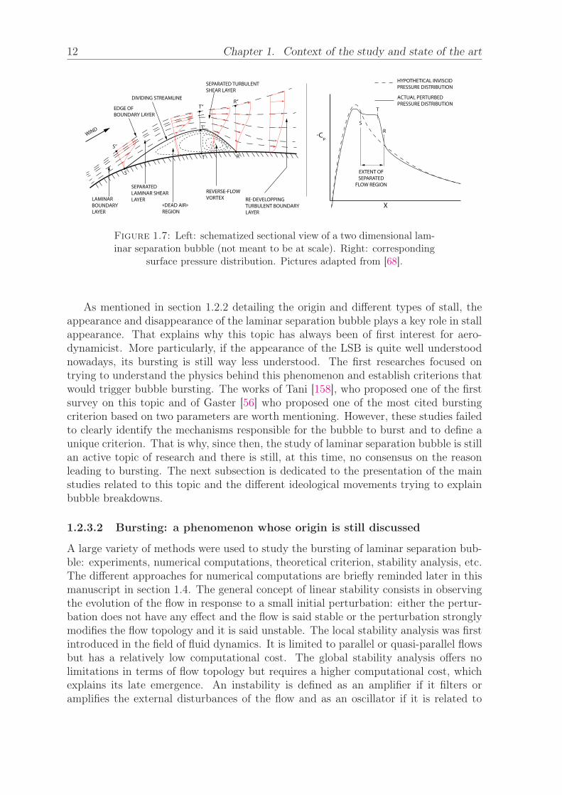
A laminar separation bubble is formed when the adverse pressure gradient in the lam-inar boundary layer is strong enough to cause flow separation (see section 1.2.1). Thenewly formed separated shear layer undergoes a transition from a laminar to a turbu-lent state. When the kinetic energy generated by the turbulent mixing is strong enoughto counter the adverse pressure gradient, the shear layer reattaches into a turbulentboundary layer. This process of separation and reattachment creates a zone, under theshear layer, called a laminar separation bubble. This zone is characterized by "dead-air" that extends from the separation point to the transition point and a reverse flowvortex at the rear of the bubble, between the transition and the reattachment points.This phenomenon is schematized in Figure (1.7), adapted from Horton [68] that ex-hibits the boundary layer formed at the curved surface of an airfoil leading edge. Thelaminar boundary layer separates at the line noted SS ′′, generating a curve ST ′R thatseparates the LSB from the shear layer. Transition occurs at the line TT ′T ′′ dividingthe shear layer into two zones: the laminar shear layer upstream this line and the tur-bulent shear layer downstream from this line. Finally, the flow reattaches at the lineRR′′ resulting in a fully attached turbulent boundary layer. This laminar separationbubble can be identified by a plateau on the pressure distribution as was shown inFigure (1.5), which describes the leading edge and thin airfoil stall mechanisms. Moreprecisely, this plateau is identified between the separation point S and the transitionpoint T and a sudden drop of pressure between the transition point T and the reat-tachment point R, as shown in Figure (1.7), which exhibits the pressure distributioncoefficient with and without LSB from Horton [68]. Owen and Klanfer [119] notedthat mostly two types of bubbles could exist: short LSB and long LSB. The secondones are at least one order of magnitude longer than the first ones. Gaster [56] notedthat the laminar parts of the shear layers are similar for short or long bubbles andalways correspond to the dead air region of the LSB. By contrast, the turbulent partof the shear layer extends as the velocity of the flow decreases. He also observed thata high frequency phenomenon is associated with the short bubble, while high and lowfrequency phenomena coexist at the same time for long LSB. Hatman and Wan [65]studied the mechanisms of the types of bubbles more in details and confirmed that thetransition is similar in both cases. They also provided more insight on the structure ofthe bubbles: the two types of bubbles reattach after the transition occurred but, in thecase of the long bubble, this reattachment is immediately followed by a new separationresulting, in the end, in a longer bubble.
12 Chapter 1. Context of the study and state of the art
-Cp
X
S
R
T
EXTENT OF
SEPARATED
FLOW REGION
HYPOTHETICAL INVISCID
PRESSURE DISTRIBUTION
ACTUAL PERTURBED
PRESSURE DISTRIBUTION
LAMINAR
BOUNDARY
LAYER
SEPARATED
LAMINAR SHEAR
LAYER
«DEAD AIR»
REGION
REVERSE-FLOW
VORTEX RE-DEVELOPPING
TURBULENT BOUNDARY
LAYER
EDGE OF
BOUNDARY LAYER
DIVIDING STREAMLINE
SEPARATED TURBULENT
SHEAR LAYER
S
S’’
R
R’’
T
T’’
T’
WIND
Figure 1.7: Left: schematized sectional view of a two dimensional lam-inar separation bubble (not meant to be at scale). Right: corresponding
surface pressure distribution. Pictures adapted from [68].
As mentioned in section 1.2.2 detailing the origin and different types of stall, theappearance and disappearance of the laminar separation bubble plays a key role in stallappearance. That explains why this topic has always been of first interest for aero-dynamicist. More particularly, if the appearance of the LSB is quite well understoodnowadays, its bursting is still way less understood. The first researches focused ontrying to understand the physics behind this phenomenon and establish criterions thatwould trigger bubble bursting. The works of Tani [158], who proposed one of the firstsurvey on this topic and of Gaster [56] who proposed one of the most cited burstingcriterion based on two parameters are worth mentioning. However, these studies failedto clearly identify the mechanisms responsible for the bubble to burst and to define aunique criterion. That is why, since then, the study of laminar separation bubble is stillan active topic of research and there is still, at this time, no consensus on the reasonleading to bursting. The next subsection is dedicated to the presentation of the mainstudies related to this topic and the different ideological movements trying to explainbubble breakdowns.
1.2.3.2 Bursting: a phenomenon whose origin is still discussed
A large variety of methods were used to study the bursting of laminar separation bub-ble: experiments, numerical computations, theoretical criterion, stability analysis, etc.The different approaches for numerical computations are briefly reminded later in thismanuscript in section 1.4. The general concept of linear stability consists in observingthe evolution of the flow in response to a small initial perturbation: either the pertur-bation does not have any effect and the flow is said stable or the perturbation stronglymodifies the flow topology and it is said unstable. The local stability analysis was firstintroduced in the field of fluid dynamics. It is limited to parallel or quasi-parallel flowsbut has a relatively low computational cost. The global stability analysis offers nolimitations in terms of flow topology but requires a higher computational cost, whichexplains its late emergence. An instability is defined as an amplifier if it filters oramplifies the external disturbances of the flow and as an oscillator if it is related to

1.2. Stall mechanisms and laminar separation bubbles 13
the flow own dynamics and do not need any external force to be triggered. The stabil-ity analysis is discussed more in detail in section 1.6 and the global stability analysisframework is defined in section 5.2.1.
The bursting of laminar separation bubble, that eventually leads to a drop of theaerodynamic performance was originally defined by Gaster [56] as the switch from ashort laminar separation bubble to a long separation bubble due to a small variation ofthe flow conditions. Actually, for finite dimensional shapes (such as airfoil), the reat-tachment of the flow can actually never occur and it results in a fully separated flow.Many criteria have been proposed and discussed to predict bubbles breakup as well asassociated phenomena such as the onset of unsteadiness or the three-dimensionalizationof the originally two dimensional LSB. But, none of the existing criteria have foundgeneral acceptance so far [43] and the mechanisms responsible for these phenomenahave started to become clearer only recently. After a lot of experimental and numeri-cal studies (mostly carried out on flat plates), two types of instabilities of the LSB areidentified: amplifier and oscillator.
The amplifier behavior of the LSB was discovered before the oscillator behavior[62] [44]. Indeed, at first, this mechanism was investigated mostly experimentally and,even in very careful experiments, the external disturbances amplitude level, thoughvery small, may be high enough to influence the dynamic of the flow. This amplifiercharacter is also identified in numerical studies by imposing an external forcing in theshape of waves. It is usually considered to account for the onset of two dimensionalunsteadiness. However, it failed to explain all the phenomena at stake (such as thethree-dimensionalization of the flow). Several papers suggested that those phenomenahad an other origin: absolute instabilities [167]. However, they could not prove it withthe tools available at the time and it was not before the drastic improvements of globalstability analysis [160] [150] that another type of behavior was proposed. In 2000,Theofilis et al. [162] were the first ones to properly apply the global stability analysisframework to a separation bubble formed on a flat plate. Two absolute instabilitieswere discovered: a two dimensional K-H instability and a three dimensional stationaryinstability. The first one was due to the amplifier behavior of the LSB while the otherone was the result of the own dynamic of the flow revealing that the LSB also had anoscillator behavior. Since then, many studies legitimately tried to determine which oneoccurs first and which one is preponderant in certain flow conditions. Rodriguez et al.[139] demonstrated that for flat-plate LSBs, the primary instability is the steady three-dimensionalisation of the bubble rather than the two-dimensional vortex shedding.
In the end, major improvements have been made on the understanding of laminarseparation bubble since the first studies. However, although two mechanisms leadingto change of flow topology have been identified, several points remain unclear. Atthis point, no one can systematically predict which mechanism will be dominating thephysics of the flow. Consequently, it remains impossible to model and anticipate how aconfiguration exhibiting a LSB will behave. Also, the link between those behaviors andLSB bursting is not directly established and fail to explain, for instance, the switch fromshort to long LSB. As a consequence, the global comprehension of laminar separationbubble remains insufficient to completely explain and predict stall. Moreover, the

14 Chapter 1. Context of the study and state of the art
literature shows the appearance of complex phenomena that seem to be related to thebehavior of LSB close to stall such as static hysteresis and low frequency oscillations.Several studies have been conducted on those phenomena but similarly to LSB andstall, their exact origin and behavior remain unclear.
1.3 Particular phenomena related to stallIn this section, we intend to present two phenomena that sometime appear aroundstatic stall and that seem to be strongly related to the existence and behavior oflaminar separation bubble.
1.3.1 Static hysteresis
-0.4
0
0.4
0.8
1.2
1.6
28.020.012.04.0-12.0-20.0
α, DEGREES
CL
-0.4
0
0.4
0.8
1.2
1.6
28.020.012.04.0-12.0-20.0
α, DEGREES
CL
(a) (b)
Figure 1.8: Evolution of the lift coefficient for: (a) a Miley M06-13-128airfoil (adapted from Pohlen et al. [129]) and (b) a Lissaman 7769 airfoil(adapted from Mueller et al. [114]) at Reynolds number Re = 150000.
The black arrows indicate the evolution of the angle of attack.
A very particular phenomenon associated with stall is the capacity of the flow to"remember" its past history and for given aerodynamic conditions have different behav-ior depending on the previous state of the flow. This phenomenon is called hysteresis.Dynamic hysteresis (which is illustrated by the dashed line in Figure (1.3)) is an ex-ample of this particular capacity of the flow as the lift values are different whetherthe angle of attack is increased of decreased. This case of hysteresis has been studiedextensively as it is of first interest in the design of helicopters (see for instance theliterature review of McCroskey [100]). However, a more reduced number of researchesfocused on the hysteresis appearing in the static stall process. The first mention ofthis phenomenon can be attributed to Schmitz [146] in his study of model of airplanewings. A classic example of static hysteresis is presented in Figure (1.8), which exhibitsthe evolution of the lift coefficient as a function of the angle of attack from (a) Pohlenet al. [129] and (b) Mueller et al. [114] for two different airfoils (respectively Miley

1.3. Particular phenomena related to stall 15
M06-13-128 and Lissaman 7769) at Reynolds number Re = 150000. The black arrowsindicate the evolution of the angle of attack. One can observe that depending if theangle of attack is increased or decreased, different states (i.e. flow topology, lift anddrag coefficients, ...) are obtained. The main difference between the two curves comesfrom the fact that Figure (a) illustrates an anticlockwise hysteresis (in which the high-est lift value is obtained for a decreasing angle of attack) while Figure (b) illustrates aclockwise hysteresis (in which the highest lift value is obtained for an increasing angleof attack). Note that in general, most of the studies exhibit a clockwise hysteresis. Inthis manuscript, except if the contrary is explicitly mentioned, hysteresis will refer toclockwise hysteresis. Mueller [113] suggested that this phenomenon is strongly relatedto laminar separation bubbles, laminar to turbulent transition and flow separation onairfoils. According to him, this would be an explanation to the inconsistency of ap-pearance of hysteresis (i.e. different results for a same airfoil and Reynolds numberreported by different authors) and the difficulty to catch it. Indeed, it was proven that achange in the freestream turbulence intensity, acoustic perturbation or Reynolds num-ber affects the appearance of static hysteresis and the size of the hysteresis loop [94].These parameters are also well known to be driving the laminar to turbulent transitionand LSB formation. The influence of the freestream turbulence level on hysteresis waslater quantified by Hoffman [67] on a NACA0015 at Reynolds number Re = 250000. Heproved that an increase of the freestream turbulence level tends to reduce the hystere-sis size. Different influences of the Reynolds number on the hysteresis were reported:for instance, Marchman et al. [93] and Mueller et al. [113] observed that the size ofhysteresis reduces with an increasing Reynolds number, while Mizoguchi et al. [111]and Selig et al. [147] observed the opposite for different airfoils. The aspect ratio ofthe wing seems also to play a key role in the formation of a hysteresis loop as provenby Marchman et al. [94] or Mizoguchi et al. [111]. Assuming that laminar separationbubbles are strongly related to hysteresis as suggested by many authors, the fact thatthe aspect ratio has an influence on the hysteresis is consistent with the results on LSBthat shows how a three dimensionnalization of the LSB is possible. The first attemptto link the behavior of the aerodynamic coefficients to the flow topology was by Yanget al. [169] who, extending the work of Hu et al. [71], studied a GA(W)-1 airfoil atReynolds number Re = 160000. They identified a hysteresis loop and found that forincreasing angles of attack, the flow is mostly attached and exhibits a laminar separa-tion bubble located at the leading edge, which causes stall when it bursts. On the otherhand, for decreasing angles of attack, the flow is first massively separated and coupledto strong vortices and turbulent structures that periodically shed in the wake. Withthe decrease of the angle of attack, the flow tries to reattach but the strong reversingflow from the trailing edge prevents it at the stall angle identified for increasing anglesof attack. In the end, reattachment occurs for an angle of attack much lower than thefirst stall angle identified, resulting in a hysteresis loop. All the aforementioned studiesobserved this phenomenon for relatively low Reynolds numbers (Re < 600000). How-ever, a few recent papers mention hysteresis at relatively high Reynods numbers. Forinstance, Broeren et al. [26], who observed it on a CRM65 semispan wing at Reynoldsnumber Re = 1.6× 10⁶ or Hristov and Ansell [70], who observed a hysteretic behaviorof the aerodynamical coefficients for a NACA0012 at Reynolds number Re = 1.0×10⁶.
In the end, this complex phenomenon appeared to be strongly related to the airfoil

16 Chapter 1. Context of the study and state of the art
shape, the Reynolds number and the quality of the flow (i.e. freestream turbulencelevel, acoustic noise,...) rendering its study very complicated. Although the exactcauses of this phenomenon are not understood at the moment, three phenomena seem tobe preponderant in its appearance: laminar to turbulent transition, laminar separationbubbles and unsteadiness occurring when the flow is separated.
1.3.2 Low frequency oscillations
The phenomenon known as low frequency oscillations (LFO) has been identified sincealmost a century as Jones [79] reported violent fluctuations of lift and drag occurringaround the angle of maximum lift at very low frequencies. However, it was only halfa century later that studies dedicated to this phenomenon were conducted. Zamanet al. [172], studying the effects of acoustic excitation on flow over an airfoil at lowReynolds number, detected a periodic wake flow structure oscillating at a Strouhalnumber based on the sine of the chord (St = f ·c·sin(α)
U∞ ) an order of magnitude lowerthan the usual bluff body vortex shedding. The name of the phenomenon comes fromthe comparison of Strouhal numbers. In an attempt to study this phenomenon morein depth, Zaman et al. [173] dedicated an experimental study to this phenomenonand identified its main features. Three airfoils, exhibiting different stall mechanismsbased on McCullough and Gault classification [102], were tested at low Reynolds num-ber (0.15 × 10⁴ < Re < 3.0 × 10⁵). The first noticeable result is that with a cleanwind tunnel, they failed to reproduce the results observed in [172]. They had to in-crease the intensity of the free-stream turbulence or to trip transition to observe theselow frequency oscillations. Then, they proved that this phenomenon has an hydro-dynamic origin, ruling out the possibility that it is due to a standing acoustic wave,a structural resonance or a blower instability. Based on this study the main featuresof this phenomenon were observed or conjectured. (a) No matter the Reynolds num-ber investigated, the Strouhal number based on the sine of the chord remains almostconstant St ≈ 0.02 and an order of magnitude lower than the usual bluff body vortexshedding St ≈ 0.2 identified in several studies including the famous paper of Rohsko[142]. (b) Large amplitude oscillations (50% of lift coefficient variation). (c) The airfoilstall type (as defined by McCullough and Gault [102]) influences the appearance ofthis phenomenon contrary to the vortex shedding unsteadiness that is independent ofthe airfoil type. Broeren et al. [24] compared twelve different shapes of airfoils andobserved that LFO were inexistant for trailing edge and leading edge stalls but couldbe identified for thin airfoil stall. However, the largest amplitude oscillations were ob-served for airfoils exhibiting coupled thin airfoil and trailing edge stall mechanisms. (d)Zaman et al. suggested that LFO could not coexist with the hysteresis phenomenon.Broeren et al. [24] argued the same in their study of twelve different types of airfoil.(e) They pointed out the leading edge as the origin of the phenomenon and observedthat the flow fluctuations are intense on the suction side of the airfoil but rapidly decaydownstream. (f) Although observed at relatively low Reynolds numbers, they arguedthat there is no reason for this phenomenon to disappear at higher Reynolds number.Bragg et al. [20] [19] confirmed this hypothesis by observing this phenomenon up toRe = 1.4 × 10⁶. They also identified that the Strouhal number of the unsteadinessslightly increases with the Reynolds number and significantly increases with the angleof attack. (g) This is a two dimensional phenomenon as confirmed by Broeren et al.

1.3. Particular phenomena related to stall 17
[25] who focused on the three dimensional phenomena occurring around stall. Theylinked the type of stall to the appearance of either LFO (thin airfoil stall or coupledthin airfoil/trailing edge stall) or stall cells [170] (trailing edge or leading edge stall).(h) They suggested that this phenomenon is linked to a transitional state and cannotappear for a laminar or fully turbulent state, which, according to them, is an explana-tion of why it is so sensitive to freestream conditions.
3603303002702402001801501209060300
0.9
1.0
0.8
0.7
0.6
0.5
0.4
0.3
0.2
0.1
0.0
x/c
Phase, φ (deg)
ReattachmentRegime
SeparationRegime
Separation bubbleRegime
Boundary-LayerSeparation Point
Leading-Edge BubbleSeparation Point
Leading-Edge Bubble Reattachment Point
Separated Boundary Layer
Attached Boundary Layer
Laminar Separation Bubble
Figure 1.9: Evolution of separation and reattachment points on thesuction side of the airfoil for one oscillation of low frequency oscillation.
Adapted from the paper of Broeren et al. [23].
After all these studies on the general features, and thanks to the improvements ofmeasurement techniques, many studies focused on the mechanism ocuring during theselarge amplitude low frequency oscillations. Broeren et al. [22] [23] identified that anoscillation can be decomposed into three regimes that are presented in Figure (1.9)(adapted from the work of Broeren [23]) showing the evolution of separation and reat-tachment points on the airfoil as a function of the phase over a period. The first regime(reattachment regime) extends from Φ = 0◦ to Φ = 165◦. It starts from a flow in afully separated state with a separation point located almost at the leading edge (∼ 10%of the chord). As the phase evolves, the separation point starts to move towards thetrailing edge, reducing the size of the separated boundary layer. The second phase(separation bubble regime) occurs from Φ = 165◦ to Φ = 255◦. It is characterized bythe appearance and expansion of a laminar separation bubble at the leading edge ofthe airfoil. In the mean time, the separation point kept moving towards the trailing

18 Chapter 1. Context of the study and state of the art
edge, reaching a maximum at Φ = 225◦ and reversed direction, moving upstream. Thethird regime (separation regime), occurring from Φ = 255◦ to Φ = 360◦, starts whenthe separation point of the boundary layer moving towards the leading edge and thereattachment point of the laminar separation bubble moving towards the trailing edgecollide, creating a massively separated flow. In the end, it results in an evolution ofthe flow over a period that switches from a stalled state (fully separated flow) to anunstalled state (mostly attached flow). Note that this scenario is a combination oftrailing edge and thin airfoil stall mechanisms combination that is known to be theone with the highest amplitude. For the airfoils exhibiting thin airfoil stall mecha-nism only, the switch between stalled and unstalled states is only generated by theexpansion, bursting and shrinkage of the laminar separation bubble. Although veryinteresting, these observations do not provide insight on the mechanism that lead theflow to reattach and the laminar separation bubble to form and expand again. A lot ofthe aforementioned studies suggested that this phenomenon is linked to the shear layerflapping and the low frequency unsteadiness identified for laminar separation bubbles(see subsection 1.2.3.2). Several studies on iced airfoils conducted by Ansell and Bragg[5] [6] [7] confirmed this theory as they identified a low frequency shear layer flappingdominating the upstream portion of the airfoil and a low frequency oscillation of theglobal circulation. However, no link could be made between these two phenomena. Thefirst attempt to precisely explain how the flow separates and reattaches was providedby Tanaka [157] who, extending the work of Rinoie and Takemura [138], noted thatwhen the flow becomes massively separated, a large vortex is generated at the leadingedge. This vortex tends to bend the shear layer towards the airfoil surface, introducingthe freestream into the separated boundary layer and tending to make the flow reat-tach. Finally, very recently, Hristov and Ansell [70] proved that the statement made byZaman et al. [173] and Broeren et al. [24] about the coexistence of hysteresis and lowfrequency oscillations might be wrong: they observed, for a NACA0012, a hysteresisloop and a low frequency phenomenon coexisting. However, the results presented morein details in Hristov PhD [69], one shall note that the amplitude of the oscillationsseems to be less large than the ones reported in most of the studies.
In the end, this complex phenomenon, similarly to hysteresis, is strongly related tothe airfoil shape and aerodynamic conditions, which both affect the airfoil stall type,as well as the existence and behavior of laminar separation bubbles. Despite the afore-mentioned studies on the subject, its origin and the mechanisms responsible for theonset of this unsteady phenomenon could not be clearly identified.
1.4 Numerical studies of stall and related phenomenaStall and associated phenomena were described in the previous sections. It is now legit-imate to wonder how numerics can help to gain an understanding of all these complexmechanisms. This is the point of this section.
Numerical simulations of complex flows are of first interest as it might offer thepossibility of studying a flow without setting up an experiment. In the particular caseof stall, assuming a perfect modeling of the flow, it could help predict the angle of attack

1.4. Numerical studies of stall and related phenomena 19
at which it might occur. However, this area is still a work in progress as complicatedmechanisms are very time and resources costly to be exactly reproduced numerically.On the other hand, alternative methods, developed to reduce the computational timeand cost, are not mature enough and fail to be reliable in all flow configurations. In theend, fluid dynamicists have to choose between computational cost and precision. Inthis section, we intend to present the different methods to numerically reproduce thebehavior of a fluid, the reasonable possibilities that can be used in the case of staticstall and, finally, how hysteresis and low frequency oscillations are treated numericallyin the literature.
1.4.1 General matters
The Navier–Stokes equations (see equations 2.1 in chapter 2) are partial differentialequations that drive the motion of a fluid, including the turbulent ones. Direct Nu-merical Simulation (DNS) consists in numerically solving these equations for all thescales of the flow. However, it faces a major drawback: in order to catch the wholephysics of the flow, all the structures, even the smallest, have to be carefully resolved.Yet, Kolmogorov showed that the size of these smallest structures diminishes as theReynolds number increases, leading to an increase of the mesh size. Based on spaceand time integration consideration, it is commonly said that the computational timefor DNS is driven by the factor Re3. In view of the nature of the flow studied inthe industry, which are almost all high Reynolds number flows, this method is onlymarginally used. An alternative method to reduce the computational cost is to filterthe smallest structures and to resolve only the largest ones. However, in order to taketheir effect into account, the smallest scales, usually associated with the turbulent ones,are modeled using a subgrid-scale model. This method is named Large Eddy Simula-tion (LES): its computational cost is reduces compared to DNS but remains quite high.Another approach is to consider a time averaged solution and model the effects of thesmall fluctuations of the flow. This is the Reynolds Averaged Navier–Stokes (RANS)approach. The influence of the fluctuations is taken into account using a turbulencemodel. This method is the most commonly encountered in the industry because ofits reduced computational time. The main drawback of modeling a part of the flow isthat the models used are usually case dependent: they might be very effective in oneprecise configuration but irrelevant in the other. Moreover, turbulence models showsome limitations as they successfully predict bypass transition but fail to reproduce anatural transition. An alternative to improve the modeling of natural transition is theuse of a so called transition model in addition to a turbulence model. However, thesemodels are difficult to calibrate and significantly increase the difficulty of the computa-tion. All these reasons explain why turbulence and transition models are still an activetopic of research. Finally, hybrid methods also exist: they consist in applying one of theaforementioned method in one zone of the flow and another in another zone of the flow.
A large number of numerical studies related to stall can be found in the literature.There is no consensus on a particular method to be used in this configuration andthe choice is always a trade-off between precision and computational time. In thecase of stall occurring at low Reynolds number, DNS can be considered. For instance,Rodriguez et al. [140] studied the flow over a NACA0012 at Re = 5 × 10⁴. The LES

20 Chapter 1. Context of the study and state of the art
approach is also well adapted to this type of flow as demonstrated by Almutairi andAlqadi on the same flow [2] or even at slightly higher Reynolds number Re = 1.3× 10⁵
by Almutairi et al. [3]. Finally, higher Reynolds number flows are resolved usinga RANS approach as in the work of Mittal and Saxena [110] who studied the flowaround a NACA 0012 at Re = 1.0× 10⁶ or a hybrid approach as in the work of Richezet al. [135] who investigated the flow around an OA209 airfoil at Re = 1.0 × 10⁶.The present work is dedicated to the study of stall at high Reynolds number with aRANS approach. As a consequence, in the remainder of the section, emphasis is puton the studies related to stall through this approach and, particularly, on the capacityof turbulence models to correctly identify and predict stall as well as static hysteresisand low frequency oscillations. However, an abundant literature, not detailed in thepresent manuscript, exists on numerical studies of stall at low Reynolds number.
1.4.2 RANS modeling of stall
One of the most studied engineering application of stall at high Reynolds number inthe literature is rotating helicopter blades. This explains why most of the studies ofstall through a RANS approach focuses on dynamic stall. Most of them comparesseveral turbulence models to experimental data, trying to identify a turbulence modelthat would correctly predict stall. Srinivasan et al. [154] compared some of the mostcommonly used and simplest turbulence models at this time (algebraic turbulence mod-els and one-equation transport turbulence models). In the end, they concluded thatalthough most of the turbulence models investigated successfully caught the global dy-namics of the flow, they all failed to correctly predict it. Some are better to modelseparated flows and other to model attached flows, but none catch all the complexityof the different flow topologies existing during the stall process. However, they notedthat the one-equation turbulence models provided better results than the algebraicones. Later, Ekaterinaris et al. [48] extended the comparison to several transport tur-bulence models (Spalart–Allmaras [151], Baldwin-Barth [9], k− ε [81], k−ω [168] andmodified versions of the k − ω model, BSL and SST by Menter [107]). The conclusionis mostly similar to the one of Srinivasan et al.: none of the investigated turbulencemodels correctly predicted stall due to their limited range of application. However,they argued that the k − ω SST turbulence model was the one providing the betterresults (an illustration of the limitation of the turbulence models is shown in Figure(3.6) in chapter 3). Finally, they noticed that, in the case of the flow is not tripped atthe leading edge, the laminar to turbulent transition plays a key role in the mechanismsoccurring at stall (as for example the formation of a laminar separation bubble). Bynature, the turbulence models, which consider a fully turbulent flow, fail to model thisregion of the flow. Indeed, a turbulent flow is less sensitive to adverse pressure gradientthat could lead to separation than a laminar flow. Consequently, the fact that the flowis already turbulent at the leading edge overestimate the capacity of the flow to remainattach delaying or even preventing a separation that is necessary to the appearanceof a laminar separation bubble. However, Ekaterinaris et al. claimed that even themost basic transition model, which considers a laminar part of the boundary layer,drastically improved the results. The conclusion of the RANS approach on modelingdynamic stall (correctly reproduce it but poorly predict it no matter the turbulencemodel) was also demonstrated in several papers for static stall [144] [137]. Finally, it is

1.4. Numerical studies of stall and related phenomena 21
worth noticing the work of Gleize et al. [61] on static stall (further extended by Szyd-lowski et al. [156] and Richter et al. [137] on dynamic stall). They demonstrated theeffect of the mesh refinement for different turbulence models, exhibiting an extremelyslow mesh convergence and a large dispersion of the results. It indicates that numericalstudies have to be carefully conducted and that the results have to be conscientiouslyverified. Indeed, coarse meshes might give results that seem in better agreement withexperiments than the ones obtained with refined mesh. However, in such a case, thisis a bias that might lead to wrong interpretation of the results.
1.4.3 Numerical studies of stall related phenomena
Although hysteresis was attributed in the literature to laminar to turbulent transitionof the boundary layer and to laminar separation bubbles, hysteresis was surprinsinglyobserved in some numerical studies performed with fully RANS computations. Mit-tal and Saxena [110] computed the flow around a NACA0012 at Reynolds numberRe = 1.0 × 10⁶ with the Baldwin-Lomax turbulence model. The unsteady RANScomputations were carried out for several angles of attack and the time-averaged val-ues of the aerodynamic coefficients were considered. They observed a static hysteresisof the aerodynamic coefficients in fair agreement with the experiments of Thibert etal. [163]. By comparing the flow visualisation at a same angle of attack, they alsoobserved stronger unsteadiness for low lift flow than for high lift flow. Richez et al.[133] computed steady solutions of a flow around an OA209 airfoil at Reynolds numberRe = 1.8×10⁶ with a k−ω turbulence model (Kok’s version with SST correction fromMenter) and observed a hysteresis of steady solutions around the stall angle. One shallnote that this hysteresis is slightly different from the ones previously described. Indeed,in experiments or in the computation performed by Mittal, the values of aerodynamiccoefficients plotted are time-averaged values deduced from unsteady solutions contraryto Richez et al. who presented values obtained from steady solutions. A similar hys-teresis of the steady solutions was also observed by Wales et al. [166] on a NACA0012airfoil at Reynolds number Re = 1.85 × 10⁶ and higher with the Edwards–Chandramodification of the Spalart–Allmaras turbulence model.
According to the author’s knowledge, there is only one paper mentioning the ap-pearance of low frequency oscillations with URANS computations. Iorio et al. [76]observed it on a NACA0012 airfoil at Reynolds number Re = 6.0 × 10⁶ and with theSpalart–Allmaras turbulent model. However, several numerical studies conducted atlower Reynolds number with LES approach provides interesting insight on the mecha-nisms of LFO at low Reynolds number. For more details, one can refer for instance tothe works of Eljack et al. [49] and the references therein.
In the end, note that although RANS and URANS computations suffer some lim-itation in correctly predicting stall, more often overestimating the stall angle, theysuccessfully identify stall but also static hysteresis and low frequency oscillations. More-over, contrary to DNS or LES, the RANS approach offers the possibility to computesteady solutions. This specific feature makes it the perfect candidate to be coupled tobifurcation theory for which steady solutions are a first requirement.

22 Chapter 1. Context of the study and state of the art
1.5 Bifurcation theoryBifurcation theory was introduced in the XV II th century by Newton in his study ofthe motion of the earth around the sun. Since then, several breakthroughs (one cancite for instance Poincaré in the XIX th century and Lorenz in the 1960’s) made thistheory dedicated to the study of dynamical system very popular in a lot of very differ-ent fields: physics, biology, electronics, chemistry, engineering, etc. The main objectiveof this theory is to identify the dependency of the system on some parameters: how dothey affect the steady states of the system, their linear stability or even the appearanceof limit cycles? Every time a qualitative change occurs in the dynamics of the system,it is said that the system faces a bifurcation and the parameter values for which it hap-pens are named the bifurcation points. Finding the bifurcation points of a system is offirst interest in order to identify the different behaviors of the system and eventuallydefining a functioning range or finding the parameters triggering the onset of a specificmechanism.
One has surely noticed that in the description of stall phenomenon made so far,the evolution of the aerodynamic coefficients or of the flow topology has always beenconsidered has a function of the angle of attack. In our attempt to study stall phe-nomenon, it would be extremely useful to identify particular values of α correspondingto sudden changes in the flow around the airfoil: instability, onset of oscillations, hys-teresis, etc. To do so, bifurcation theory will be considered with the angle of attackas a parameter. Several types of bifurcations will be encountered in this manuscript,such as saddle-node bifurcations of steady states and limit cycles, Hopf bifurcationsand homoclinic bifurcations as well as the notions of attractors and repellers. One canfind a detailed description of these notions in the abundant literature on this topic andfor instance to the books of Strogatz [155] or Gilmore [60].
Bifurcation theory was applied to fluid dynamics to understand the physics of flowin many configurations. An extensive review of bifurcation theory applied to Navier–Stokes equations and the discoveries resulting from this formalism can be found inthe review of Dijkstra et al. [41]. As examples, one can mention several papers whoaddressed the different behaviors of flows by varying the Reynolds number: Barkleyet al. [11] on a circular cylinder, Nagata [115] on a plane Couette flow, Mamun andTuckerman [92] on a spherical Couette flow, Fabre et al. [51] on a sphere and a flatdisk, Meliga et al. [105] on a flat disk or Cui et al. [34] who, based on the polar curvesobtained by Mueller [113] on a Lissaman 7769, identified the bifurcation leading to theformation of hysteresis. Moreover, several studies are directly related to the study ofstall considering the angle of attack as the bifurcation parameter. Dimitriadis and Li[42] adressed the question of stall flutter, identifying different flow behavior as the angleof attack varies. Wales and Gaitonde [166] studied static stall on a NACA0012 at highReynolds number and partially established the bifurcation diagram by computing thesteady solutions using continuation methods identifying a hysteresis of steady solutionsand two saddle-node bifurcations.
As stated by Tuckerman and Barkley [165], any CFD code is sufficient to performa bifurcation analysis of a flow. Indeed, a stable state (steady or limit cycle) can be

1.6. Global linear stability analysis 23
reached after a long enough time and by gradually shifting a control parameter, one canobserve when the flow changes and identify the bifurcation points. However, it suffersseveral limitations: the impossibility to reach unstable steady states, the difficulty toidentify specific phenomena such as unstable limit cycles, and, particularly, it mightbe extremely time costly to wait for stabilization or destabilization of certain states.To overcome these difficulties, several specific tools, dedicated to bifurcation theorywere developed. For instance, continuation methods, linear stability analysis, Floquetstability analysis or nonlinear stability analysis, respectively used for the computationof steady states, the study of their stability, the study of limit cycles stability andthe determination of bifurcation criticality. Note that the implementation of all thesemethods in the RANS framework is not an easy task.
1.6 Global linear stability analysisLinear stability analysis is a very powerful tool in the bifurcation theory framework.It was proven to be very useful in the study of laminar separation bubble (as detailedin subsection 1.2.3.2) and, coupled with a RANS approach, it is expected to providevery interesting insights on stall, static hysteresis and LFO. In this section we intendto detail the global stability analysis principles (briefly detailed in subsection 1.2.3.2)as well as its application to turbulent flows modeled with a RANS approach.
The concept of instabilities in fluid mechanics has been existing for over a hundredyears and the most famous examples are probably the Kelvin-Helmotz instability andthe Benard-von Karman vortex street. The concept of linear stability analysis, de-veloped to study those instabilities, is very commonly used in the field of dynamicalsystems. It consists in determining how a small perturbation of the initial conditionaffects a system: does it or does it not change its actual state? If, after a long time,the perturbation has not affected the system, it is said stable, otherwise the system issaid unstable. Considering the flow as a system, such an analysis applied to the fieldof fluid dynamics shall help to have a better understanding of the onset of unsteadyphenomena. At first, the local stability analysis was considered due to its reduced com-putational time (see for example the works of Batchelor and Gill [12] or Crighton andGaster [31]). This approach considers that the flow does not vary in the streamwisedirection and a crosswise profile completely describe the flow topology. This way, onlythe cross-stream direction of the flow is to be considered and discretized. However, italso limits its domain of application to parallel and quasiparallel flows, which wave-length of the unsteady phenomena is short compared to the typical streamwise scaleof the flow. Studying the propagation of the local instabilities, Huerre and Monkewitz[72] classified them into two categories: absolutely unstable or convectively unstable.For absolute unstable flows, the perturbation remains located at its origin and only ex-pands upstream and downstream without moving while for convective unstable flows,the perturbation is convected far away from the source while expanding. With theincrease of computational power, a new approach was recently considered: the globalstability analysis (also referred as Bi-Global or Tri-Global stability in some paper forrespectively two and three dimensional flows). This approach has been widely usedin the field of fluid dynamics (see for instance the literature reviews of Theofilis [160][161], Sipp et al. [150] or Chomaz [29]) as it can be used for any flow configuration

24 Chapter 1. Context of the study and state of the art
contrary to the local stability analysis. However, the computational cost is obviouslyhigher. A mathematical description of this theory is given in section 5.2.1. Huerre andMonkewitz [72] also adressed the question of comparing local and global approaches.They argued that an absolute local instability is a necessary condition for the existenceof a global instability. Another very commonly used classification associated with lin-ear stability analysis is the distinction between oscillators and amplifiers. A flow issaid to act as an oscillator if it imposes its own dynamic at a very particular frequency,independent of the external noise. This type of instability is associated with an un-stable global mode (defined by Drazin [45] as a state variable in which the dynamicof the system is driven by coherent oscillations). A flow is said to act as an amplifierif the external disturbances coming from upstream are filtered or amplified when con-vected downstream. This type of instability is associated with a global stable modewhich requires other techniques to be identified (see for instance the work of Cossu [30]).
Although being in constant development with the increase of the computationalcapacities, global stability analysis still suffers computational limitations to study com-plex three dimensional configurations. The mathematical framework presented in sec-tion 5.2.1 is perfectly usable for three dimensional flows and several studies, which havesuccessfully performed global stability analysis of three-dimensional configurations, ex-ist in the literature (see for instance Tezuka and Suzuki [159] Bagheri et al. [8] or morerecently Paladini [122]). However, results found in the literature demonstrated thatall the phenomena that we intend to study can be identified with a two dimensionalstudy. Consequently, in order to reduce the computational cost, the choice is made tostudy the global stability of a two dimensional flow.
One of the main question related to the linear stability analysis is: around whichflow the equations should be linearized? Stability of dynamical systems considers thesteady state of the system as base flow around which the equations are linearized. Thisapproach is mathematically more accurate. However, in the case of the Navier–Stokesequations, experiments and Direct Numerical Simulation do not permit to considersuch a base flow. In these cases, mean flows (i.e. time averaged solutions) are usuallyconsidered, which raises a lot of questions in the field of stability analysis applied tofluid mechanics. Several studies showed surprisingly good results with global stabilityanalysis of mean flows (for instance Barkley [10] or Piot et al. [127]) and extendedstudies were dedicated to the identification of conditions for the use of mean flows (forinstance Sipp and Lebedev [149] or Beneddine et al. [15]). The case of linear stabilityanalysis applied to RANS flows is a bit different but raises the same kind of questions.Indeed, it is possible to compute steady RANS solutions around which perform linearstability analysis. However, because of the inherent properties of the RANS approxi-mation, a steady solution of the RANS equations is not necessarily a steady solution ofthe Navier–Stokes equations as it is already a time averaged solution. If the theoreticalframework and rigorous validation for the use of linear stability analysis coupled withRANS approach has not been established, several studies exhibited very good resultsfor various configurations such as the buffet (which has been one of the most studiedtopic with for instance the works of Crouch et al. [32] [33], Sartor et al. [145], Iorio etal. [75], Paladini et al. [123],...) or the deep cavity flow by Mettot et al. [108]. Finally,the work of Iorio et al. [76] is worth mentioning: their main objective was the global

1.6. Global linear stability analysis 25
stability analysis of a turbulent flow around a complex multielements airfoil but, in avalidation step of the method, they presented very interesting insights on the stabilityanalysis of a turbulent flow around a NACA0012 at low Mach number M = 0.15 andReynolds number Re = 6.0 × 10⁶ with the Spalart–Allmaras turbulence model. Theanalysis revealed an unstable global mode (illustrated in Figure (1.10)) which associ-ated frequency is very low. The existence of such an unsteadiness was confirmed withunsteady RANS computations with an excellent agreement between the frequencies.
Figure 1.10: Structure of the unstable global mode found for the flowaround a NACA0012 at low Mach number M = 0.15 and Reynolds num-ber Re = 6.0 × 10⁶ with the Spalart–Allmaras turbulence model. (a)Streamwise velocity component (b) Turbulent component. From the pa-
per of Iorio et al. [76].
If the global stability analysis allows the user to identify the type of instabilitygoverning the flow, the most sensitive regions of the flow are a very useful informationto obtain and several methods were developed for this purpose. The adjoint modeis the easiest information to obtain from a linear global stability analysis. For eachglobal mode (also called direct mode), a corresponding eigenvalue, which real partcorresponds to the growth rate and imaginary part to the angular frequency of the in-stability, is found. It is also possible to determine a so-called associated adjoint mode(the mathematical formalism of the adjoint mode is introduced in section 5.2.5.1). Thephysical meaning of the adjoint mode is the designation of the zones where an externalforcing will be the most effective to amplify or damp the instability of the associateddirect mode [148]: the most receptive regions of the flow. Consequently, it is of firstinterest when intending to control the instability mechanism. Emphasis were also puton finding the regions of the flow that affect the most the eigenvalue (i.e. the temporalproperties of the instability). With that goal in mind, Huerre and Monkewitz [72]proposed the concept of wavemaker, which was extended by Giannetti and Luchini [59]who proposed a formalism that nowadays meet consensus in the community. In thesame spirit, Paladini et al. [123], extending the work of Marquet and Lesshaft [95],proposed an alternative tool based on the decomposition of the linear operator instead(by opposition to the approach of Giannetti and Luchini [59] who considered a pertur-bation of the linear operator). The method, called eigenvalue contribution, providesa density function which real (respectively imaginary) part shows the influence of the

26 Chapter 1. Context of the study and state of the art
flow on the growth rate (respectively angular frequency). The contribution of the flowcan be either positive or negative contrary to the wavemaker function which is definedas a norm. Furthermore, it is proven in the PhD of Paladini [122] that from the eigen-value contribution, it is possible to determine the wavemaker function highlighting thelink between the two approaches. These two tools are mathematically introduced insubsection 5.2.5.1.
1.7 The OA209 airfoilThe previous sections introduced the problematic of stall, its link with helicopter per-formance and the limitations of our comprehension of this phenomenon as well as statichysteresis and LFO. The different methods that can be used to model this phenomenonwere also introduced, as well as bifurcation theory and linear stability analysis widelyused in the field of fluid dynamics nowadays. In our attempt to apply those tools tothe specific case of stall, a particular helicopter blade airfoil is used: the OA209. Thissection intends to present the results that can be found in the literature on this airfoilin the aerodynamic conditions considered (i.e. a retreating blade configuration at Machnumber M = 0.16 and Reynolds number Re = 1.8× 10⁶).
The OA209 is a helicopter blade airfoil that was designed in the 70’s at ONERA.This airfoil is still in service on several helicopters. As explained in section 1.1.2, dy-namic stall plays a key role in helicopters performance. This explained why so manystudies were carried out on this topic at ONERA. For many of them, the OA209 airfoilwas used, which gives us a lot of information about the flow topology, the aerodynamicperformance and the phenomena occurring. Although the aim was to study dynamicstall, many studies address the question of static stall as it is very helpful to understandthe complex dynamical phenomena. At first, an experimental database was formed byPailhas [121] et al. and widely extended by Le Pape et al. a few years later [125].Several Reynolds numbers were investigated (Re = 0.5 × 10⁶, Re = 1.0 × 10⁶ andRe = 1.8 × 10⁶). It appeared that a diminution of the Reynolds number leads to adiminution of the stall angle and the maximum lift coefficient. Also, the two lowestvalues revealed the appearance of a laminar separation bubble at the leading edge.They noted that the higher the Reynolds number, the lower the size of the recircu-lation bubble (which is in agreement with the observations of O’Meara and Mueller[118]). According to them, this diminution of the size with the increase of the Reynoldsnumber is the reason why this LSB is not identified at Re = 1.8 × 10⁶ as they sug-gested that the pressure probes refinement might be too large to identify a tiny LSB(< 1% of the chord) in that case. They also noted that a very classic laminar to tur-bulent transition is associated with this LSB. Richez et al. [134] performed a hybridRANS/LES computation at Re = 1.8×10⁶ on a prior stall configuration and confirmedthe appearance of a laminar separation bubble at the leading edge (although they sug-gested that its size is overestimated in their computation). Several numerical studieson a post-stall configuration at Re = 1.0 × 10⁶ [136] [135] and Re = 1.8 × 10⁶ [136]revealed the appearance of vortex shedding occurring at St ≈ 0.2 when the flow is fullydetached. In terms of modeling, two points are worth noticing. First, Jain et al. [78]demonstrated that the fully turbulent RANS approach constantly overestimates the

1.8. Objectives and outline 27
stall angle and the Spalart–Allmaras turbulence model appears to be even worse thanthe k − ω model (note that the overprediction was already noticed by Richter et al.[137] for the Spalart–Allmaras model). Second, Kaufman et al. [85] noted on a flow atRe = 1.0× 10⁶ that, with the Spalart–Allmaras model, only a trailing edge separationappeared, characteristic of a trailing edge stall, contrary to experiments that exhibit acoupled leading edge/trailing edge stall. Finally, Richez et al. [133] computed steadyRANS solutions with the k − ω turbulence model and identified a static hysteresis ofsteady solutions around stall. Figure (1.11) illustrates this hysteresis by showing theevolution of the lift coefficient of steady solutions as a function of the angle of attackclose to stall angle: for several values of α, a high lift solution coexists with a lowlift solution. Note that this hysteresis is different from the one illustrated in Figure(1.8): this one is a hysteresis of steady solutions while the other one is a hysteresis oftime-averaged unsteady solutions.
α(° )
CL
17.4 17.6 17.8 18
1
1.2
1.4
1.6
0.8
Figure 1.11: Evolution of the lift coefficient as a function of the angleof attack. Obtained from steady RANS computations with the k −ω turbulence model for an OA209 at M = 0.16 and Re = 1.8 × 10⁶.Identification of a static hysteresis of steady solutions close to stall angle.
Adapted from Richez et al. [133].
1.8 Objectives and outlineThe aim of the present study is to provide more insight into stall phenomenon in anattempt to improve helicopters’ performance. By opposition to static stall (encoun-tered in the case of airplanes for instance), the blades of a helicopter face dynamic stall,which is caused by inertia effects generated by the variation of theirs angles of attackduring one rotation. It is shown in the literature that the dynamic stall characteristicsof an airfoil are driven by its static stall properties [128]. In the present work, the choiceis made to neglect the dynamic effects of stall and to focus on static stall, which alsoremains not well understood. The aerodynamic conditions corresponding to the case of

28 Chapter 1. Context of the study and state of the art
a retreating blade perpendicular to the helicopter fuselage are used for the static com-putations because they correspond to the most critical configuration regarding stall. Itis characterized by a low Mach number and high Reynolds number flow, which raisesthe question of the numerical approach to be considered in this work. Because of thehigh Reynolds number, the choice of a RANS approach is made in order to be able tocompute several solutions at a reasonable computational cost and in a realistic time.The turbulence model chosen is the Spalart–Allmaras model and no transition modelis used, which is well known to provide decent results in the case of static stall [121],although not as good as the k − ω model coupled with a transition model for instance[48]. Two main reasons motivated this choice: the relative simplicity of the turbulencemodel (one equation), which facilitates the implementation part and the fact that lowfrequency oscillations and static hysteresis can be identified with this turbulence model[166] [76], which allows us to gain an understanding of those phenomena even with thissimple modeling.Moreover, the present work also intends to take advantage of the capacity of the RANSformalism to compute steady solutions, which are a prerequisite to perform a studythrough bifurcation theory. Although the first steps of a bifurcation scenario aroundstall were proposed in several papers, a complete bifurcation diagram was never drawn.One can refer to Wales et al. [166] who computed steady solutions around stall usingcontinuation methods and study their linear stability but did not focus on the bifurca-tions occurring or to Iorio et al. [76] who identified a low frequency stable mode closeto stall but only focused on the study of high lift solutions and did not track the modeall along the curve. In the present work, it is intended to go further with the followingstrategy: (i) couple continuation methods to the RANS formalism (ii) conduct a morecareful linear global stability analysis of the steady solutions (iii) perform unsteadyRANS computations to investigate the nonlinear behavior of the flow and (iv) createa one-equation stall model to gain an understanding of the nonlinear phenomena thatcannot be identified with the standard unsteady RANS computations. With such anapproach, we intend to answer several questions: does an unstable mode responsiblefor stall exist? How does this mode evolve along the polar curve as the angle of attackvaries? What are the most sensitive regions of the flow at stall? How may the lowfrequency oscillations and hysteresis, which are mentioned in several studies in the lit-erature, be linked to the behavior of this mode? Can we explain why these phenomenasometimes appear at stall and sometimes not? And, can we draw a bifurcation diagramthat would logically link all these phenomena?
To answer these questions, the particular case of a two dimensional OA209 airfoilin retreating blade configuration (i.e. M = 0.16 and Re = 1.8 × 10⁶) is considered atfirst. The RANS approach coupled with the Spalart–Allmaras turbulence model [151]is retained to perform this study of this high Reynolds number flow. Chapter 2 is ded-icated to the presentation of the numerical tools used: RANS formalism, turbulencemodel, numerical schemes and definition of residuals.Chapter 3 is dedicated to confirm that stall, static hysteresis and low frequency oscil-lations, which were all identified for different flow configurations, airfoils or turbulencemodel, can be observed with the Spalart–Allmaras turbulence model in the configu-ration studied by varying the angle of attack from α = 12.00◦ and α = 22.00◦. Thestandard time stepping methods implemented in the CFD solver elsA [27] is used. A

1.8. Objectives and outline 29
local time stepping approach is used to compute steady solution: the results obtainedwith the Spalart–Allmaras model are similar to the ones found in the literature. More-over, it is proven that the static hysteresis identified in this configuration with thek−ω turbulence model by Richez et al. [133] is also caught with the Spalart–Allmarasturbulence model. Similarly to Iorio et al. [76] on a NACA0012 at Re = 6.0× 10⁶, anunsteady RANS computations with the Spalart–Allmaras turbulence model reveal alow frequency oscillation for one particular angle of attack in the high lift configurationclose to stall. Finally, this chapter is also the opportunity to highlight the limitationsof time steppers to study stall.Once it has been proven that stall, static hysteresis and low frequency oscillations canbe found in this configuration with the Spalart–Allmaras turbulence model, the mainquestion is to know if it is possible, similarly to the work of Wales and Gatonde [166] ona NACA0012, to identify a branch of unstable steady solutions, unaccessible with thelocal time stepping approach, which would link the two branches of respectively highlift steady solutions and low lift steady solutions. To answer this question, continuationmethods are necessary. These methods will also allow us to override the convergenceproblems of time steppers close to stall angle. Chapter 4 introduces the formalism oftwo continuation methods (the naive continuation method and the pseudo arclengthmethod [86]) and their implementation in association with the CFD solver elsA [27].These methods are applied to the flow configuration mentioned by considering the an-gle of attack α as the parameter of the study. The results, presented in the first part ofchapter 5, show that it is possible to identify a branch of steady solutions that link thetwo already computed upper and lower branches, similarly to the results of Wales et al.[166]. The stability analysis of each steady solution in the range of 12.00◦ < α < 22.00◦
is investigated. The second part of chapter 5 is dedicated to the presentation of thetwo unstable modes encountered: a stall mode (similar to the one identified by Iorioet al. [76]) and a vortex shedding mode. Their associated adjoint modes and differentsensitivity analysis [91] [123] are also presented. In the last part of chapter 5, theevolution of the stall mode along the polar curve is presented and several bifurcationsare identified.Chapter 6 is dedicated to the identification and tracking of unsteadiness and limit cy-cles with URANS simulations: a large low frequency limit cycle is encountered aroundstall and a vortex shedding unsteadiness is identified for high angles of attack, both ingood agreement with the results of the linear stability analysis. A first proposition ofbifurcation scenario taking limit cycles into account is made but the lack of informationavailable with this method is highlighted.It was mentioned in section 1.5 that studying the bifurcations of a system with timesteppers is possible but quite limited [165]. Ideally in order to complete the informa-tion obtained in chapter 6, it would be interesting to develop a tool able to track limitcycles [39]. However, in order to avoid the development of a supplementary tool aone-equation stall model is used. This nonlinear model, presented in chapter 7 is basedand calibrated on the evolution of the steady states and their linear behavior describedin chapter 5. The study of the nonlinear behavior of this models is supposed to replacethe tracking of the limit cycles identified with URANS computations and provide usadditional information. This approach is a considerable gain of time and computa-tional ressource as specific softwares and plugin, such as Matcont [39], already existto study in detail the bifurcations of simple systems such as this one. Based on this

30 Chapter 1. Context of the study and state of the art
one-equation model, a plausible complete bifurcation scenario involving saddle-nodebifurcations, subcritical Hopf bifurcations and Homoclinic bifurcations that would linkstall, low frequency oscillations and hysteresis is proposed. Another advantage of thisapproach is the possibility to study slightly different cases at a very low computationalcost by varying the constants of the model, which allowed us to propose alternativebifurcation scenarios.Finally, in chapter 8, a different Reynolds number and a different airfoil are inves-tigated to verify if the bifurcation scenario observed can be encountered in differentconfigurations.

31
Chapter 2
Standard tools to study stall throughRANS approximation
Contents2.1 The RANS formalism . . . . . . . . . . . . . . . . . . . . . . 31
2.1.1 Compressible Navier–Stokes equations . . . . . . . . . . . . . 31
2.1.2 The Reynolds Averaged Navier–Stokes formalism . . . . . . . 33
2.1.3 Spalart–Allmaras turbulence model . . . . . . . . . . . . . . . 36
2.1.4 Edwards–Chandra modification of the Spalart–Allmaras tur-bulence model . . . . . . . . . . . . . . . . . . . . . . . . . . . 37
2.2 Numerics . . . . . . . . . . . . . . . . . . . . . . . . . . . . . 38
2.2.1 elsA, a finite volume software . . . . . . . . . . . . . . . . . . 38
2.2.2 Spatial discretisation . . . . . . . . . . . . . . . . . . . . . . . 39
2.2.3 Temporal approach . . . . . . . . . . . . . . . . . . . . . . . . 41
2.2.4 Residuals . . . . . . . . . . . . . . . . . . . . . . . . . . . . . 44
The principle advantages and drawbacks of the RANS approach have been discussed inthe introduction. In this chapter we intend to introduce the mathematical formalismof the approach as much as the Spalart–Allmaras turbulence model. The solver andthe numerical schemes used to perform time marching computations are introduced forsteady and unsteady computations.
2.1 The RANS formalism
2.1.1 Compressible Navier–Stokes equations
In continuum mechanics theory, which implies that the smallest scale of the flow islarger than the molecular scale, the Navier–Stokes equations are believed to describethe physics of all fluid flows including the turbulent ones. They were introduced inthe mid XIXth century by the mathematician Henry Navier and the physicist GeorgeGabriel Stokes. In the case of a compressible, viscous and heat conductor flow and by

32 Chapter 2. Standard tools to study stall through RANS approximation
neglecting the effects of the gravity, the local form of these equations can be written asshown in equations (2.1) in cartesian coordinates using the Einstein notation. Theseequations describe respectively the mass conservation, the momentum equation andthe energy conservation.
⎧⎪⎪⎪⎪⎪⎪⎪⎨⎪⎪⎪⎪⎪⎪⎪⎩
∂ρ
∂t+
∂
∂xj
(ρuj) = 0
∂
∂t(ρui) +
∂
∂xj
(ρuiuj) = − ∂p
∂xi
+∂τij∂xj
i = 1, 2, 3
∂
∂t(ρE) +
∂
∂xj
[(ρE + p)uj] =∂
∂xj
(τijui)− ∂qj∂xj
(2.1)
where t is the time variable and xi the ith spatial coordinate. The variables ρ designatethe density, ui the ith component of the flow speed, p the static pressure, τij a componentof the the stress tensor , qi the ith component of the heat flux and E the total energy.To close this system, the expression of some variables needs to be set.
2.1.1.1 Energy
The total energy E is defined as the sum of the internal energy e and the kinetic energyper mass unit.
E = e+1
2uiui (2.2)
2.1.1.2 Ideal gas law
In the case where the fluid can be considered as an ideal gas, the ideal gas law linksthe pressure p with the density ρ in equation (2.3) where T designates the temperatureof the fluid, r the ratio of the universal gas constant R = 8.3145J.mol−1.K−1 to themolar mass M of the flow considered (r = M
R).
p = ρrT (2.3)
This law also links the pressure p to the internal energy e in equation (2.4) whereγ is the ratio of isobaric to isochoric heat capacities (γ = Cp
Cv). For a diatomic gas,
γ = 1.4.
p = ρ(γ − 1)e (2.4)
2.1.1.3 Stress tensor
The hypothesis of a Newtonian fluid is made to express the stress tensor τ . It meansthat the tensor is linked to the strain tensor (depending on the velocity derivatives

2.1. The RANS formalism 33
with respect to the position) through a viscosity tensor that does not depend on thestress state and velocity of the field. In the case of an isotropic fluid, this viscositytensor can be reduced to two real coefficients. It leads to equation (2.5) where μ andλ are the coefficients of the viscosity tensor.
τij = λ∂uk
∂xk
(δij) + μ
(∂ui
∂xj
+∂uj
∂xi
)(2.5)
The Stokes hypothesis is considered verified and a link between the two coefficientscan be made : λ+ 2
3μ = 0.
τij = −2
3μ∂uk
∂xk
(δij) + μ
(∂ui
∂xj
+∂uj
∂xi
)(2.6)
Finally, the coefficient μ can be deduced from the Sutherland’s law. It links theviscosity to the temperature only, respecting the Newtonian fluid hypothesis.
μ(T ) = μ0
(T
T0
) 32 T + 110.4
T0 + 110.4(2.7)
where T0 = 273.16K and μ0 = 1.711× 10⁻⁵kg.m−1.s−1 for air.
2.1.1.4 Heat flux
Fourier’s law links the heat flux to the temperature gradient as shown in equation (2.8).
qi = −κ∂T
∂xi
(2.8)
where κ is set by using the definition of the Prandtl number (equal to Pr = 0.72 for air),which is a dimensionless number characterizing the ratio between the viscous diffusionrate and the thermal diffusion rate. It leads to equation (2.9) where μ and Cp havealready been defined.
κ =μCp
Pr(2.9)
2.1.2 The Reynolds Averaged Navier–Stokes formalism
At high Reynolds number, the use of Direct Numerical Simulations (DNS) to solvethe Navier–Stokes equations (2.1) is extremely costly, which makes this method almostimpossible, particularly for industrial problems. One alternative is the Reynolds Av-erage Navier–Stokes (RANS) approach, which consists in modeling the lowest scalesof the turbulence with a so called turbulence model. This section is dedicated to thedecomposition of the Navier–Stokes equations (presented in (2.1)) into the ReynoldsAveraged Navier–Stokes equations. The average operator as defined first by Reynolds

34 Chapter 2. Standard tools to study stall through RANS approximation
[132] is introduced, as well as the decomposition applied to the Navier–Stokes equa-tions. The reader can refer to the book of Gatski and Bonnet for more details aboutthis formalism [57].
2.1.2.1 Average operator
The RANS approach considers turbulence as a random phenomenon that can be studiedfrom a statistical point of view. The main hypothesis of this approach is that eachvariable f of the flow can be decomposed into a mean part 〈f〉 and a fluctuating partf ′.
f = 〈f〉+ f ′ (2.10)
where 〈f〉 is the ensemble average of the variable f , which corresponds to the meanvalue of the variables fk after a number N of independent realizations in the sameconditions.
〈f〉 = 1
N
N∑k=1
fk (2.11)
To be formally exact, one should consider N → ∞. However, such a limit con-siderably complexifies the mathematical framework besides being not realistic, as inpractice, a finite number of experiments would have to be considered. This operatorfollows Reynolds properties (a being a scalar and ψ a time or space variable) :
〈f ′〉 = 0 〈f + g〉 = 〈f〉+ 〈g〉 〈a.f〉 = a.〈f〉〈〈f〉〉 = 〈f〉 〈fg〉 = 〈f〉〈g〉+ 〈f ′g′〉 〈∂f
∂ψ〉 = ∂〈f〉
∂ψ
〈〈f〉g〉 = 〈f〉〈g〉
2.1.2.2 Averaged equations
Equation (2.10) was introduced by Reynolds for turbulent incompressible flows. How-ever, in order to simplify the notations for the case of compressible flows, the Favreaverage [53] [54] is introduced :
f = f + f ′′ with f =ρf
ρ(2.12)
By applying this decomposition to the system (2.1), it becomes:

2.1. The RANS formalism 35
⎧⎪⎪⎪⎪⎪⎪⎪⎪⎪⎪⎪⎪⎪⎪⎪⎪⎪⎪⎪⎪⎪⎪⎪⎨⎪⎪⎪⎪⎪⎪⎪⎪⎪⎪⎪⎪⎪⎪⎪⎪⎪⎪⎪⎪⎪⎪⎪⎩
∂ρ
∂t+
∂
∂xj
(ρui) =0
∂ρui
∂t+
∂
∂xj
(ρuiuj + pδij − τ ∗ij) =− ∂
∂xj
(ρ˜u′′i u
′′j )
+∂
∂xj
(τ ij − τij)
∂
∂t(ρE) +
∂
∂xj
(ρEuj + puj − τ ∗ijui + q∗j ) =− ∂
∂xj
((ρe′′ + p)u′′j )
− ∂
∂xj
(ρ˜u′′i u
′′j ui) +
∂
∂xj
(τiju′′i ) +
∂
∂xj
(τ ijui − τ ∗ijui)
+∂
∂xj
(1
2ρu′′
i u′′i u
′′j
)− ∂
∂xj
(qj − q∗j )
(2.13)
with:
ρE = ρe+1
2ρuiui +
1
2ρ ˜u′′
i u′′i
τ ∗ij = −2
3μ(T )
∂uk
∂xk
δij + μ(T )
(∂ui
∂xj
+∂uj
∂xi
)
q∗i = −κ(T )∂T
∂xi
(2.14)
(2.15)
(2.16)
In order to simplify the set of equations (2.13), two hypotheses are made : theinfluence of viscosity fluctuations in the viscous stress tensor is neglected as well as theeffects of the fluctuations of the density [112]. It leads to the following set of equations:⎧⎪⎪⎪⎪⎪⎪⎪⎪⎨
⎪⎪⎪⎪⎪⎪⎪⎪⎩
∂ρ
∂t+
∂
∂xj
(ρui) = 0
∂ρui
∂t+
∂
∂xj
(ρuiuj + pδij − τ ∗ij) = −∂τRij∂xj
∂
∂t(ρE) +
∂
∂xj
(ρEuj + puj − τ ∗ijui + q∗j ) = −∂qRtj∂xj
− ∂
∂xj
(τRij ui)
(2.17)
where τRij is the Reynolds stress tensor and qtiR the viscous heat flux defined by:
τRij = −ρ˜u′′i u
′′j
qtiR = (ρe′′ + p)u′′
j
(2.18)
(2.19)
Note that at this stage, this system has more unknowns than equations: closureequations are required to solve system (2.17). The simplest closure equations are firstorder models. The concept is to add a set of equations that links the two turbulent

36 Chapter 2. Standard tools to study stall through RANS approximation
variables τRij and qtiR to the mean values of the flow instead of computing them with
costly transport equations. The first order Boussinesq approximation is chosen in ourcase for the Reynolds stress tensor:
τRij = μt
(∂ui
∂xj
+∂uj
∂xi
− 2
3
∂uk
∂xk
δij
)− 2
3ρkδij (2.20)
where k is the kinetic energy of the viscous fluctuations, such as: k = 12
˜u′′i u
′′i . For the
turbulent heat flux, a Reynolds analogy is used:
qtj = −κt∂T
∂xi
(2.21)
where κt is defined using the Prandtl number:
κt = −μtCp
Prt(2.22)
Finally, the variable μt is the only unknown that remains to be defined in this setof equations. The point of turbulence models is to provide additional equations todefine this quantity. Two types of turbulence models exist: algebraic turbulence modeland transport equations turbulence model. In this PhD thesis, the Spalart–Allmarasmodel, which is a one equation transport turbulence model, is used. The next sectionis dedicated to its description.
2.1.3 Spalart–Allmaras turbulence model
This turbulence model, designed especially for aeronautic application, is based on asingle transport equation for the kinetic eddy turbulent viscosity and was created bySpalart and Allmaras [151] and adapted to compressible flows by Deck [38]. Theequation is built empirically, using dimensional analysis and studying four differentflows to add more complexity to the model. It starts with simple free shear flowsfrom which the simplest version of the model is designed based on the general form:Convection = Production − Dissipation + Diffusion. Correction terms were added toobtain a logarithmic velocity profile in the near wall region at high Reynolds number.Then, additional corrections were made to correctly describe the buffer layer and vis-cous sublayer at low Reynolds number. Finally, some terms were provided to trip theboundary layer transition and trigger turbulence. Equation (2.23) presents the finalform of the model in the compressible case.
⎧⎪⎪⎪⎪⎪⎪⎪⎪⎨⎪⎪⎪⎪⎪⎪⎪⎪⎩
μt = ρνfv1
D(ρν)
Dt= Cb1(1− ft2)Sρν +
Cb2
σ
∂ρν
∂xj
∂ν
∂xj
− (Cw1fw − Cb1
κ2ft2)ρ
ν2
d2− ∂
∂xj
[1
σ(μ+ ρν)
∂ν
∂xj
] (2.23)

2.1. The RANS formalism 37
where the terms used are described as follow (d being the distance to the wall) :
fv1 =χ3
χ3 + C3v1
ft2 = Ct3eCt4χ2
χ =ρν
μ
S = ||−→rot−→U ||+ ν
κ2d2fv2 fv2 = 1− χ
1 + χfv1
fw = g
(1 + C6
w3
g6 + C6w3
)g = r + Cw2(r
6 − r) r =ν
Sκ2d2
with the recommended values for the constants :
Cb1 = 0.1355 Cb2 = 0.622 σ =2
3κ = 0.41
Cw1 =Cb1
κ2+
(1 + Cb2)
σ= 0.3 Cw2 = 2 Cv1 = 7.1 Ct1 = 1
Ct2 = 2 Ct3 = 1.1 Ct4 = 2
This model offers a good balance between simplicity and efficiency. Its one equa-tion form leads to reduced computational time and it was proven to be very robust.However, it shows some limits in complex configurations.
2.1.4 Edwards–Chandra modification of the Spalart–Allmarasturbulence model
The modification of the Spalart–Allmaras turbulence model proposed by Edwards andChandra [46] was originally made to solve convergence issues close to the leading edgestagnation point. The singular behavior of the source term S in the near-wall regionand the implicit formulation of the equation on the ν variable (see equation (2.23)) arethe main reason of such convergence issues. The modification consists in redefining thesource term S and the parameter r as presented in equations (2.24) to (2.26). Also,the ft2 term is ignored.
S = S12
[1
χ+ fv1
](2.24)
with
S =
(∂ui
∂xj
+∂uj
∂xi
)∂ui
∂xj
− 2
3
(∂uk
∂xk
)2
r =tanh
(ν
S2κ2d2
)tanh(1.0)
(2.25)
(2.26)

38 Chapter 2. Standard tools to study stall through RANS approximation
2.2 Numerics
2.2.1 elsA, a finite volume software
There are several possibilities to resolve numerically partial derivative equations (PDE):finite volume method, finite element methods, finite difference, ... The CFD solver usedat ONERA, elsA [27], is based on the finite volume method. Contrary to the finitedifference method, based on an approximation of the derivative, the finite volume andelement methods are based on approximations of integrals. The finite volume methoduses the strong form of the equations whereas the finite element method uses the weakform of the equations. Using the Green-Ostrogadski theorem, the integral form ofequations (2.1) and (2.23) can be written under the generic integral form presented inequation (2.27).
d
dt
∫Ω(t)
qdΩ +
∮∂Ω(t)
[F c + Fd] · n(t)dΣ =
∫∂Ω(t)
T dΩ (2.27)
where Ω(t) is the computation domain, ∂Ω(t) the boundary of outer normal n(t), F c
and Fd the convective and diffusive fluxes respectively, T designates the source termsand q = [ρ, ρu, ρv, ρw, ρE, ρν] the solution of the compressible Navier–Stokes equationsin the RANS framework coupled with the Spalart–Allmaras turbulence model. Theapproximation of a fixed and unalterable domain is also set. The point of the finitevolume method is to obtain an approximated solution of the equation (2.27) by using amesh made of several separated finite volumes, which once reunited correspond to thewhole domain. The equation is solved in each domain (cell) Ωcell of volume V (Ωcell)and of boundary surface (resp. line) Σi defined such as :
V (Ωcell) =
∫Ωcell
dΩ and ∂Ωcell =N∑i=1
Σi
where N corresponds to the number of adjacent cells. The structural solver of theCFD code elsA is used in this PhD thesis. Consequently, for the remainder of thesection, the cells will be considered to be hexahedra. Each surface Σi has a normal nand the outer norm of the cell is defined such as NΣi
=∫ΣindΣ. In the case of the
cell-centered formulation, considered in elsA, the values of the variables of q the fluxesand the source terms are constant in each cell and are defined such as:⎧⎪⎪⎪⎪⎪⎪⎪⎨
⎪⎪⎪⎪⎪⎪⎪⎩
qcell =1
V (Ω)
∫Ωcell
qdΩ
F Σi=
∮Σi
[F c + Fd] · ndΣ
T cell =1
V (Ω)
∫∂Ωcell
T dΩ
(2.28)
(2.29)
(2.30)
Finally, equation (2.27) becomes (2.31) for a cell :

2.2. Numerics 39
V (Ω)d
dtqcell = −Rcell with Rcell =
N∑i=1
F Σi− V (Ω)T cell (2.31)
R being the local residual of the cell. The method presented offers several advan-tages and drawbacks briefly introduced here. The finite volume method in itself offersthe advantage of being completely independent of the mesh. However, the attributesof the mesh are of first importance in the correct evaluation of the fluxes. The cell-centered method offers the advantage of a good precision on the results as the volumeused in the integral correspond exactly to the volume of the mesh. However, it requiresan interpolation to apply the boundary condition. A key step in the success of thismethod is the method of computation of the fluxes. Several methods exist and in thenext subsection, the ones used in our case are introduced.
2.2.2 Spatial discretisation
In order to simplify the indexation, the numerical schemes are presented in this sectionfor the case of a one dimensional mesh pictured on figure (2.1). The center of thereference cell i is at a position xi. The boundaries of the cell are at positions xi−1/2
and xi+1/2 (corresponding to the position of the nodes).The index i+1/2 is used to referto any quantity at the boundary in xi+1/2.
Vi
Vi-1
Vi+1
qi
qi+1
qi-1
xi+1
xi
xi-1
xi+1/2
xi-1/2
Figure 2.1: Cell-centered discretization in a one dimensional case.
2.2.2.1 Convective fluxes for conservative variables
The convective fluxes of the conservative equations (2.1) are discretized using theAUSM+(P) scheme [47], a modified version of the AUSM+ scheme. The name ofthe original scheme stands for Advection Upstream Splitting Method, which, practi-cally, means that the flux is considered to have two physically distinct parts: convectiveand pressure fluxes. Several modification were introduced to improve the robustnessand the accuracy of the model as much as the applicability domain (speed-regimes,phases,...). The AUSM+(P) ensures a good precision for all flow speeds (from super-sonic to low Mach number configurations). However, in our configuration of low Mach

40 Chapter 2. Standard tools to study stall through RANS approximation
number, the capture of shock properties is useless and so a modified version of origi-nal AUSM+(P) scheme, from [99], is used in order to reduce the computational time.Finally, the expression of the flux at the boundary xi+1/2 is defined in equation (2.32).
F ci+1/2 =
1
2U1(W
Li+1/2 +WR
i+1/2)−1
2|Udis|(WR
i+1/2 −W Li+1/2) + P (2.32)
where exponents R and L refers to the interpolating values on the right and on the left ofthe boundary respectively, U1 is the flow speed at the interface, W is a state vector suchas W = (ρ, ρu, ρv, ρw, ρE+p), the pressure term P is defined by P = (0, (p
L+pR)2
, 0, 0, 0)and Udis, introduced as a local flow speed, characterizes the numerical dissipation actingon the velocity components. These quantities are defined by :⎧⎪⎪⎪⎪⎪⎪⎪⎪⎪⎪⎨
⎪⎪⎪⎪⎪⎪⎪⎪⎪⎪⎩
U1 =1
2(uL + uR)− c2(p
R − pL)
Udis = max
(1
2|uL + uR|, c1
)
W Li+1/2 = W i +
1
6[2(W i+1 −W i) + (W i −W i−1)]
WRi+1/2 = W i+1 − 1
6[2(W i+1 −W i) + (W i+2 −W i+1)]
The term c2(pR − pL) in the expression of U1 is a stabilization term introduced to
improve the velocity/pressure coupling in the low mach number regions. c1 and c2 aretwo constant values set to c1 = c2 = 0.04 in order to minimize dissipation and ensurestability as recommended in the PhD Thesis of Mary [98] (which also contains a preciseanalysis of the behavior of this numerical scheme). The expressions of the left and rightinterpolated values are defined by using the reconstruction scheme MUSCL developedby Van Leer [90] (standing for Monotonic Upstream Schemes for Conservation Laws),in the case of a partially non-centered third order scheme.
2.2.2.2 Convective fluxes for turbulent variables
In order to discretize the fluxes appearing in the turbulent equation (2.23), the noncen-tered Roe scheme is used [141]. This scheme is based on a linearisation of the Riemannproblem. The expression of the flux at the boundary xi+1/2 is defined in equation(2.33):
F ci+1/2 =
1
2
[F c(qLi+1/2) + F c(qR
i+1/2)− |ARoe|(qLi+1/2 + qR
i+1/2)]
(2.33)
Where ARoe is the diagonalisable Jacobian matrix such that |ARoe| = M |λi|IM−1,λi designating the eigenvalues of ARoe and M the transformation matrix. However,too low eigenvalues could lead to nonentropic solutions. To prevent such a behavior,Harten and Hyman [64] proposed a modification of the scheme such as the entropyissue is fixed.

2.2. Numerics 41
2.2.2.3 Diffusive fluxes
The diffusive fluxes are by definition easier to compute. The same cell-centered schemebased on a five points stencil is used for the conservative and turbulent equations. Inthe case of the one dimensional formalism introduced in Figure (2.1), it leads to:
F di+1/2 =
1
2(F d
i+1 + F di )
F di−1/2 =
1
2(F d
i + F di−1)
(2.34)
The gradients required to compute the source terms are estimated at cell centersusing the Ostrogradski formula:
∂F d
∂xk
∣∣∣∣i
≈ 1
V (Ω)
∫∫∫Ωi
∂F d
∂xk
dΩi =1
V (Ω)
∫∫Σi
F dndΣi (2.35)
2.2.3 Temporal approach
2.2.3.1 Schemes
Two approaches can be considered for the numerical time integration of the Navier–Stokes equations : explicit or implicit methods. The first one calculates the solutionat an iteration n + 1 from the state at iteration n. It results an easy formulation andimplementation and a reduced computational cost. However, the explicit methods re-quires small time steps Δt in order to ensure the stability of the scheme. The implicitmethod is more complex as it requires to solve a system in which the current state atiteration n and the expected solution at iteration n + 1 are coupled. It results in amuch more difficult implementation and a higher computational cost. However, thisscheme is unconditionally stable, which leads to the possibility to use higher time stepsthan the explicit method.
In the case of the explicit method, the time step Δt is chosen by using the Courant-Friedrich-Lewy condition (CFL) defining in equation (2.36). It links the size of meshΔx to the time step Δt via V the the modulus of the mean velocity in the cell, c thelocal sound speed in the cell and some fluid parameters already defined. The CFLcondition, defined in these terms, takes into account the convective and dissipativeparts of the flow (two terms in the min operator) and only the most critical is used todetermine the step time Δt. The CFL parameter is also introduced: it is a coefficientthat must satisfy CFL〈1 in the case of an explicit scheme.
Δt ≤ CFL ×min
⎡⎣ Δx
V + c,
ρ(Δx)2
2γ(
μ
Pr +μt
Prt
)⎤⎦ (2.36)
With such a condition on the explicit schemes, one can obviously notice that smallcells will lead to small time steps. Yet, to correctly model the physics of the boundary

42 Chapter 2. Standard tools to study stall through RANS approximation
layer with a RANS approach, very small cells are required. This observation leads usto consider an implicit approach.
The computation of steady solutions (RANS) is performed by considering an un-steady computation with a local time stepping approach. It means that, as the historyof the solution is not of interest, different time step Δt are used for each cell, directlydetermined from the CFL condition. It means that small time steps are used in smallcells and larger time steps are used in larger cells. It allows the destruction of unsteadi-ness that could lead to oscillatory phenomena and a reduced computational time. Wechoose CFL = 30 to scale the local time step Δt in our RANS computations.
In the case of unsteady computations (URANS), the history of the flow is requiredand consequently the method of local time stepping is useless. Note that in that case,the choice of an explicit scheme would have been even more critical as the choice ofthe time step Δt is global and scaled on the smallest cell of the mesh. In the case ofan implicit scheme, we just ensure that the time step is small enough compared to thefrequency of the physical phenomena we intend to observe.
Finally, two different implicit schemes are chosen for the steady and unsteady cases.First, a backward Euler scheme (first order scheme presented in equation (2.37) ob-tained from equation (2.31)) is used for steady computations.
qn+1cell − qn
cell
ΔtV (Ω) = −Rn+1
cell (2.37)
Second, a Gear scheme (second order scheme presented in equation 2.38 obtainedfrom equation (2.31)) is used for unsteady computations .
3qn+1cell − 4qn
cell + qn−1cell
2ΔtV (Ω) = −Rn+1
cell (2.38)
In both cases, we intend to find the solution qn+1 at iteration n+1 corresponding toa time (n+1)·Δt (local or global depending on the type of computation) by consideringqn and qn−1 known. The residual Rn+1
cell is defined as the some of the all the fluxes andproduction terms of the cell (see equation (2.31)). In both cases, it leads to a systemof the form :
G(qn+1) = 0 (2.39)
where qn+1 is a vector of dimension Nvariables ×Nx ×Ny ×Nz
2.2.3.2 Resolution of the non linear problem
Steady case
To resolve equation (2.37), the residual Rn+1cell is first linearized in equation (2.40).
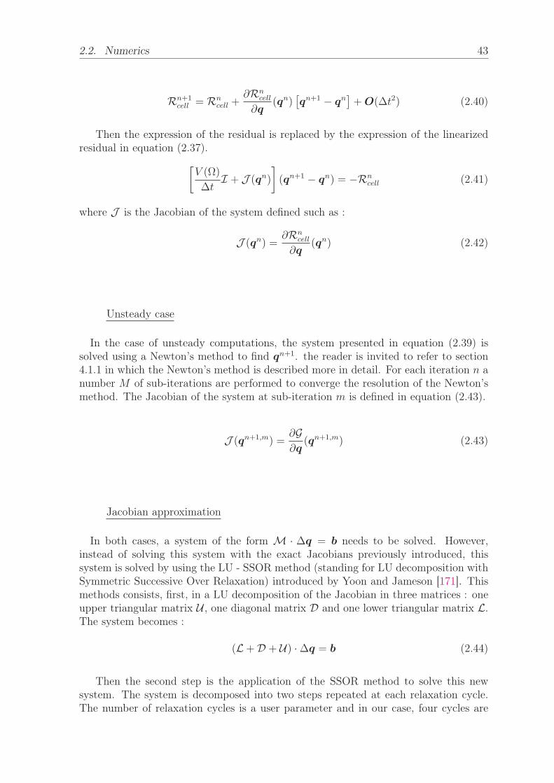
2.2. Numerics 43
Rn+1cell = Rn
cell +∂Rn
cell
∂q(qn)
[qn+1 − qn
]+O(Δt2) (2.40)
Then the expression of the residual is replaced by the expression of the linearizedresidual in equation (2.37).[
V (Ω)
ΔtI + J (qn)
](qn+1 − qn) = −Rn
cell (2.41)
where J is the Jacobian of the system defined such as :
J (qn) =∂Rn
cell
∂q(qn) (2.42)
Unsteady case
In the case of unsteady computations, the system presented in equation (2.39) issolved using a Newton’s method to find qn+1. the reader is invited to refer to section4.1.1 in which the Newton’s method is described more in detail. For each iteration n anumber M of sub-iterations are performed to converge the resolution of the Newton’smethod. The Jacobian of the system at sub-iteration m is defined in equation (2.43).
J (qn+1,m) =∂G∂q
(qn+1,m) (2.43)
Jacobian approximation
In both cases, a system of the form M · Δq = b needs to be solved. However,instead of solving this system with the exact Jacobians previously introduced, thissystem is solved by using the LU - SSOR method (standing for LU decomposition withSymmetric Successive Over Relaxation) introduced by Yoon and Jameson [171]. Thismethods consists, first, in a LU decomposition of the Jacobian in three matrices : oneupper triangular matrix U , one diagonal matrix D and one lower triangular matrix L.The system becomes :
(L+D + U) ·Δq = b (2.44)
Then the second step is the application of the SSOR method to solve this newsystem. The system is decomposed into two steps repeated at each relaxation cycle.The number of relaxation cycles is a user parameter and in our case, four cycles are

44 Chapter 2. Standard tools to study stall through RANS approximation
considered in the steady case and two in the unsteady case. By introducing the numberof the cycle p, the final system to be solved is :
{(L+D) ·Δqp+1/2 = b− U ·Δqp
(D + U) ·Δqp+1 = b− U ·Δqp+1/2
(2.45)
(2.46)
2.2.4 Residuals
Depending on the type of computation, elsA can provide several types of residual,which are introduced in the present subsection.
2.2.4.1 Explicit residual
The explicit residual, is based on the definition of the residual of the cell as the sumof all the fluxes and production terms of the cell introduced in equation (2.31). Ascalar value of the residual for each variable qi of the solution vector q is obtained byconsidering the square root of the mean value of the squared local residual value Ri
cell
weighted by the volume of the cell V (Ω) as shown in equation (2.47).
Resn+1explicit(qi) =
√√√√ 1
N
N∑k=1
(Ricell
V (Ω)
)2
(2.47)
2.2.4.2 Implicit residual
The explicit expression of the residual might struggle to correctly estimate the realconvergence of the computation when an implicit method with large time steps areused. An alternative definition of the residual based on the solution increment insteadof an evaluation of the right hand side is considered and leads to equation (2.48). Thisis the type of residual used to analyze convergence in our unsteady computations.
Resn+1implicit(qi) =
√√√√ 1
N
N∑k=1
(qi,n+1cell − qi,ncell
Δt
)2
(2.48)
2.2.4.3 Explicit/implicit residual
A third option, coupling both approaches is also possible. This explicit/implicit ver-sion, available for RANS computations with a transport equations turbulent model,consists in using the explicit definition of the residual for the conservative equationsand the implicit definition of the residual for the turbulent equations. This way, theapplication of limiters on the turbulence variables, which is possible only with the im-plicit computation, can be taken into account. This is the type of residual used toanalyze convergence in our steady computations.

45
Chapter 3
The OA209 airfoil in stallconfiguration: a standard toolsapproach
Contents3.1 Nondimensionalization, mesh and boundary conditions . . 45
3.2 Steady solutions of the RANS equations coupled with theSpalart–Allmaras model . . . . . . . . . . . . . . . . . . . . 48
3.2.1 General overview of the solutions . . . . . . . . . . . . . . . . 48
3.2.2 Presentation of the polar curves . . . . . . . . . . . . . . . . . 50
3.2.3 Convergence of the steady solutions . . . . . . . . . . . . . . 52
3.2.4 Discussion of the results obtained . . . . . . . . . . . . . . . . 53
3.3 Unsteady RANS computations . . . . . . . . . . . . . . . . 54
3.4 Conclusion . . . . . . . . . . . . . . . . . . . . . . . . . . . . . 56
In this chapter, we intend to apply the methods and tools described in chapter 2 (i.e.a time stepping approach in the RANS formalism coupled with the Spalart–Allmarasturbulence model). The particular case of a two dimensional OA209 airfoil at Re =1.8 × 10⁶ and M = 0.16, corresponding to a retreating helicopter blade configuration,is investigated. The objective is to identify a stall mechanism by varying the angleof attack of the airfoil. First, the airfoil, the mesh and the boundary conditions areintroduced. Then, the results of the steady and unsteady computations are presentedand analyzed. Finally, the limitations of this approach are discussed.
3.1 Nondimensionalization, mesh and boundary con-ditions
For the aforementioned aerodynamic conditions, we intend to solve the Navier–Stokesequations (2.13) coupled with the Spalart–Allmaras turbulence model (2.23). Thissystem is written in the form dq
dt= R(q) where the vector solution q has the following

46 Chapter 3. The OA209 airfoil in stall configuration: a standard tools approach
variables q = (ρ, ρu, ρv, ρE, ρν)T . Where ρ is the density, u the streamwise velocityin the horizontal axis (x0), v the cross-stream velocity in the vertical axis (y0), E theinternal energy and ν the turbulent variable (the axes x0 and y0 are introduced inFigure (3.1) and detailed below). All the quantities are made non-dimensional withrespect to the chord c and the speed of sound A = 340m · s−1 and are presented asunitless in this manuscript except if explicitly mentioned.
x
y
x0
y0
α
α
(a) (b)
(c)
Figure 3.1: Visualization of the mesh around a two dimensional OA209airfoil. (a) Whole domain with boundary conditions A and B. (b) Zoomin close to the airfoil with boundary condition C. (c) Zoom in close to
the trailing edge, highlighting the sharp angle.
Figure (3.1) shows three views of the mesh used : (a) exhibits the whole domain(of approximately twenty times the chord length on each direction), (b) shows a zoomin close to the airfoil and (c) presents a zoom in close to the trailing edge. Particularattention has been paid to the refinement close to the airfoil (as shown in Figure(3.1)(b)) in order to correctly capture the physics of the boundary layer. Also, aneffort has been made to try to ensure as much as possible the local perpendicularitybetween the lines starting from the airfoil and the boundary C. In the end, this mesh ismade of 144352 cells. Also, looking at the bottom right picture of Figure (3.1), one canobserve how the trailing edge has a sharp angle. Such a geometry is not representativeof the real geometry but this approximation of a zero thickness of the trailing edge ismade in order to simplify the remainder of the study. Finally, the airfoil reference frame(x0,y0) is also defined in Figure (3.1) as well as the flow reference frame (x,y). Thissecond reference frame is introduced to model the inclination of the airfoil. Indeed, weintend to compute solutions for a large range of angles of attack (12.00◦ < α < 22.00◦)and, instead of rotating the airfoil and generating a new mesh for each value of α,

3.2. Steady solutions of the RANS equations coupled with the Spalart–Allmarasmodel 47
the inclination of the airfoil is modeled through the boundary conditions. On theboundary condition A, a compressible inlet condition is set, such that the flow speedis u∞ = U∞x. This leads to the following flow quantities on A in the airfoil referenceframe (x0,y0):
q∞ =
⎛⎜⎜⎜⎜⎝
ρ∞U∞ cos(α)U∞ sin(α)
E∞ν∞
⎞⎟⎟⎟⎟⎠ (3.1)
where ρ∞ = 1 (deduced from the Reynolds number and Sutherland’s law (2.7) beforebeing non-dimensionalized to be equal to one), U∞ = 0.16 (non-dimensionalized byA such that U∞ = M∞), E∞ is deduced from the equations of the total energy (2.2)and the ideal gas law (2.4) (non-dimensionalized by the square of the speed of soundA2) and ν∞ = 3ν∞, based on the recommendation from Spalart and Rumsey [152] andnon-dimensionalized by ρ∞, A∞ and the chord. In the end, the boundary condition Ais driven by the angle of attack α and can be written q∞ = f(α). On the boundarycondition B, a compressible outlet condition is set and an adiabatic wall conditionis imposed on boundary condition C. One shall note that the computations are per-formed in the airfoil reference frame (x0,y0) but all the results are presented in theflow reference frame (x,y).
In order to identify the capacity of the mesh to capture the physics of the bound-ary layer, one can evaluate the number of cells in the viscous sublayer by using thedimensionless parameter y+ defined in equation (3.2) where y is the height of the firstcell, τw the wall shear stress, ρ the density and ν the viscosity.
y+ =yuτ
νwhere uτ =
√τwρ
(3.2)
The evolution of the y+ value around the airfoil is plotted as a function of thepercentage of the chord on the pressure side (dashed line) and the suction side (solidside) for four angles of attack (α = 12.00◦, α = 16.00◦, α = 18.00◦ and α = 22.00◦) inFigure (3.2).
Note that the condition y+ < 1 is always validated on the suction side permittingan accurate computation of the viscous sublayer. The values on the pressure side areslightly higher but remain correct (y+ < 2.5) as the characterization of the pressureside is not as critical as the suction side.

48 Chapter 3. The OA209 airfoil in stall configuration: a standard tools approach
y+
0 0.5 1
0.5
1
1.5
% of chord % of chord0 0.5 1
0.5
1
1.5
2
% of chord
y+
0 0.5 1
0.5
1
1.5
2
% of chord0 0.5 1
0.5
1
1.5
2
2.5
(a) (b)
(c) (d)
Pressure side
Suction side
Pressure side
Suction side
Pressure side
Suction side
Pressure side
Suction side
Figure 3.2: Evolution of the y+ value as a function of the percentageof the chord for the flow around a OA209 airfoil at Re = 1.8 × 10⁶
and M = 0.16. (a) α = 12.00◦. (b) α = 16.00◦. (c) α = 18.00◦. (d)α = 22.00◦.
3.2 Steady solutions of the RANS equations coupledwith the Spalart–Allmaras model
3.2.1 General overview of the solutions
Figure (3.3) shows the ρu field (left) and the ρν field (right) for different angles ofattack. In each picture, the limit of the recirculation bubble, if existing, is plotted ina black line. For each case, the position of the corresponding angle of attack is indi-cated with a red dot on the middle picture showing the evolution of the lift coefficientas a function of the angle of attack. This curve is presented and discussed more indetails in Figure (3.4). The first angle of attack investigated in pictures (a) and (b) isα = 12.00◦. For this value of α, the flow is fully attached and there is no recirculationbubble. The wake is relatively thin and the level of turbulence in it is extremely low.The second case, α = 16.00◦, depicted in pictures (c) and (d), exhibits the appearanceof a tiny recirculation bubble at the trailing edge. The thickness of the wake, the levelof turbulence as well as the lift coefficient increase with the angle of attack. The nextconfiguration, α = 17.50◦, presented on pictures (e) and (f) corresponds to a maximum
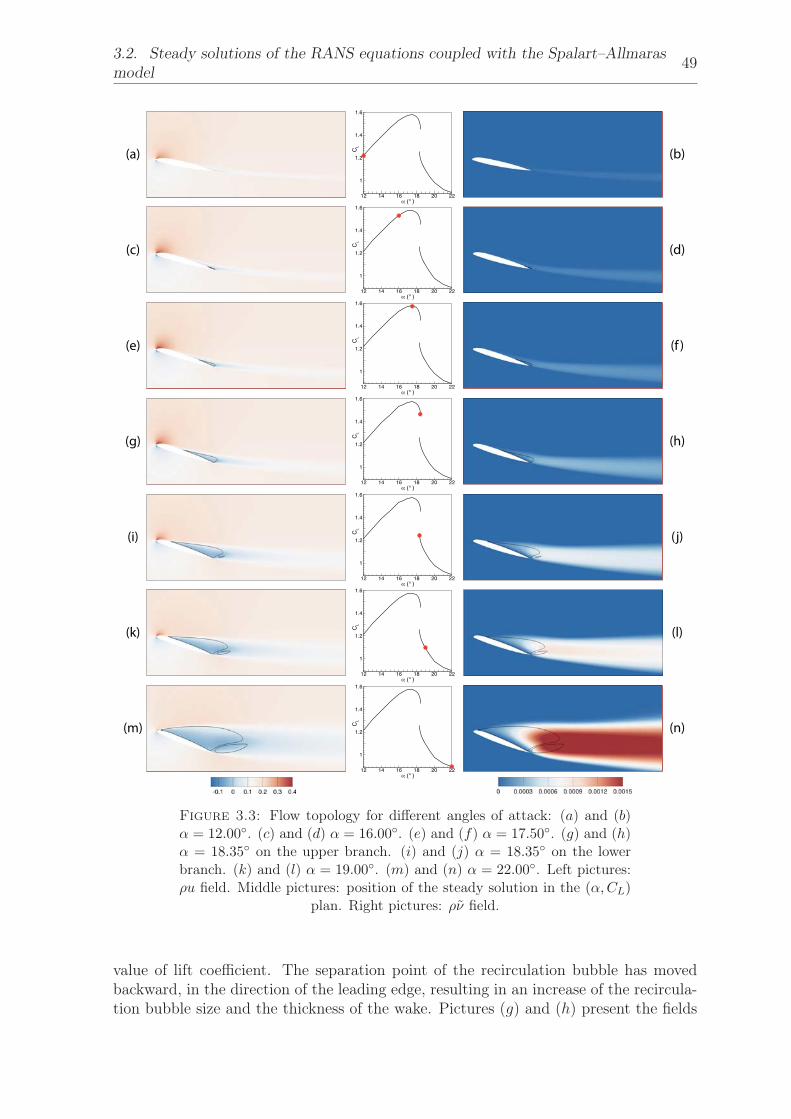
3.2. Steady solutions of the RANS equations coupled with the Spalart–Allmarasmodel 49
α (° )
CL
12 14 16 18 20 22
1
1.2
1.4
1.6
α (° )
CL
12 14 16 18 20 22
1
1.2
1.4
1.6
α (° )
CL
12 14 16 18 20 22
1
1.2
1.4
1.6
α (° )
CL
12 14 16 18 20 22
1
1.2
1.4
1.6
α (° )
CL
12 14 16 18 20 22
1
1.2
1.4
1.6
α (° )
CL
12 14 16 18 20 22
1
1.2
1.4
1.6
α (° )
CL
12 14 16 18 20 22
1
1.2
1.4
1.6
(a) (b)
(c) (d)
(e) (f )
(g) (h)
(i) (j)
(k) (l)
(m) (n)
Figure 3.3: Flow topology for different angles of attack: (a) and (b)α = 12.00◦. (c) and (d) α = 16.00◦. (e) and (f) α = 17.50◦. (g) and (h)α = 18.35◦ on the upper branch. (i) and (j) α = 18.35◦ on the lowerbranch. (k) and (l) α = 19.00◦. (m) and (n) α = 22.00◦. Left pictures:ρu field. Middle pictures: position of the steady solution in the (α,CL)
plan. Right pictures: ρν field.
value of lift coefficient. The separation point of the recirculation bubble has movedbackward, in the direction of the leading edge, resulting in an increase of the recircula-tion bubble size and the thickness of the wake. Pictures (g) and (h) present the fields

50 Chapter 3. The OA209 airfoil in stall configuration: a standard tools approach
for α = 18.35◦ just before a sudden drop of lift. The separation point kept moving to-wards the leading edge and the recirculation bubble size as well as the thickness of thewake increased. The same angle of attack α = 18.35◦ is presented in pictures (i) and(j) but the flow topology is completely different : the flow is now massively separated,resulting in a much bigger recirculation bubble and wake thickness as well as a largerturbulence level in the wake. Also, a second small recirculation bubble appears at thetrailing edge. The coexistence of these steady solutions was introduced in chapter 1and was expected considering the work of Richez et al. [133]. A new interpretation,enlightened by the continuation method approach, is presented in detail afterwards insubsection 5.1.2. Then, the case α = 19.00◦ is presented in pictures (k) and (l). Theevolution of the recirculation bubble and the wake is similar to the one observed sofar. Moreover, the small recirculation zone at the trailing edge also grows and, bydoing so, pushes the reattachment point of the large recirculation bubble towards theleading edge. Finally, the highest angle of attack investigated, α = 22.00◦, is presentedin pictures (m) and (n). The flow is now massively separated from almost the leadingedge and the modelled turbulence level is high. In the end, the evolution of the flowtopology is characteristic of a trailing edge stall as the separation point moves towardthe leading edge as the angle of attack is increased. This result is in good agreementwith the prediction of Kaufman et al. who noticed that computations performed witha fully turbulent Spalart–Allmaras model caught the trailing edge separation but omit-ted the laminar separation bubble at the leading edge suggesting a trailing edge stallmechanism instead of a coupled leading edge/trailing edge stall.
From all these solutions, it is possible to extract some aerodynamic coefficients thatcan be plotted as a function of the angle of attack and provide a quantitative evolutionof the flow. These coefficients are defined in appendix A.
3.2.2 Presentation of the polar curves
Figure (3.4) shows the evolution of the lift coefficient (a) and (b), the drag coefficient (c)and (d) and the pitching moment coefficient (e) and (f). The three left pictures (a), (c)and (e) show the evolution of the coefficients for 12.00◦ < α < 22.00◦ while the middlepictures (b), (d) and (f) exhibit a zoom in for the area 18.28◦ < α < 18.43◦. One canfirst observe in pictures (a), (c) and (e), a linear increase of the lift, drag and pitchingmoment coefficients for the lowest values of angles of attack (from 12.00◦ to 17.50◦
approximately). Then stall occurs, characterized by a sudden drop of lift and pitchingmoment coefficients and a sudden increase of the drag coefficient. Finally, the lift andpitching moment coefficients keep decreasing more slowly after stall occurs while thedrag coefficient keeps increasing. One can observe a discontinuity of the evolution of thethree aerodynamic coefficients computed from the steady solutions. This discontinuityoccurs precisely at stall. Based on this discontinuity, two different branches of the curveare defined: the upper branch that corresponds to steady solutions between α = 12.00◦
until stall and the lower branch that corresponds to steady solutions between stall andα = 22.00◦. The name of the branches is based on the value of the lift coefficient thatis generally larger for the upper branch than for the lower branch. Moreover, a veryinteresting phenomenon is observed close to stall (presented in pictures (b), (d) and

3.2. Steady solutions of the RANS equations coupled with the Spalart–Allmarasmodel 51
α(° )
CL
12 14 16 18 20 220.9
1
1.1
1.2
1.3
1.4
1.5
1.6
α(° )
CM
12 14 16 18 20 22
-0.8
-0.6
-0.4
-0.2
0
α(° )
CD
12 14 16 18 20 22
0.1
0.2
α(° )
CM
18.3 18.35 18.4
-0.3
-0.2
-0.1
0
α(° )
CL
18.3 18.35 18.4
1.2
1.3
1.4
1.5
α(° )
CD
18.3 18.35 18.4
0.06
0.08
0.1
0.12
(b)
(d)
(f )
(a)
(c)
(e)
Upper branch
Lower branch
Upper branch
Lower branch
Upper branch
Lower branch
(h)
(g)
h
g
h
g
h
g
Figure 3.4: Evolution of several flow topology related values of steadysolutions as a function of the angle of incidence. (a) and (b) Evolutionof the lift coefficient. (c) and (d) Evolution of the drag coefficient. (e)and (f) Evolution of the pitching moment coefficient. (g) and (h) Flowvisualisation of the ρu field for α = 18.35◦ on the upper branch (g) and
the lower branch (h).
(f)), at the discontinuity: the two branches overlap for 18.30◦ < α < 18.41◦ for allthe aerodynamic coefficients. It means that, for this range of angles of attack, twodifferent steady solutions coexist for each value of α. This is illustrated in pictures (g)and (h), which show the flow for the ρu variable for α = 18.35◦ on the upper and lowerbranches. The associated aerodynamic coefficients associated with these two solutionsare marked in pictures (b), (d) and (f). The numerical procedure to identify sucha phenomenon is based on the initialization of the RANS computations: to computethe upper (respectively lower) branch, one shall first compute a steady solution for anangle of attack α lower (respectively higher) than the angles of attack for which twosteady solutions coexist. Then a steady solution is computed for α+Δα (respectivelyα−Δα) and so on until the end of the branch is reached. It is considered done when,for a small enough increment Δα, the computation for α+Δα gives a steady solution

52 Chapter 3. The OA209 airfoil in stall configuration: a standard tools approach
on the other branch. This means that, by numerically increasing the angle of attack(upper branch) or by numerically decreasing it (lower branch) different solutions arereached, which is typical of a hysteresis phenomenon.
3.2.3 Convergence of the steady solutions
Itérations
Exp
licit re
sidu
al :
ρu
0 500000 1E+06
10-8
10-4
10012.0018.0018.39 upper branch18.31 lower branch19.0022.00
Itérations
Impl
icit re
sidu
al :
ρν
0 500000 1E+06
10-16
10-12
10-8
10-4 12.0018.0018.39 upper branch18.31 lower branch19.0022.00
Itérations
Exp
licit re
sidu
al :
ρu
0 50000 100000 150000
10-4
100 12.0018.0018.39 upper branch18.31 lower branch19.0022.00
Itérations
Impl
icit re
sidu
al :
ρν
0 50000 100000 150000
10-8
10-4
12.0018.0018.39 upper branch18.31 lower branch19.0022.00
(a) (b)
(c) (d)
˜˜
Figure 3.5: Evolution of the residual for the variables ρu (explicit)and ρν (implicit) for six different values of α on a log scale. (a) and (b):evolution for 106 iterations. (c) and (d) evolution for the beginning of
the computation.
Figure (3.5) presents the evolution of the explicit residual of the variable ρu andthe implicit residual of the variable ρν on a log scale for several angles of attack. Asa reminder, for the local time stepping computations, the residual type used is theexplicit/implicit type, which means the explicit residuals is considered for the con-servative variables, while the implicit residual is considered for the turbulent variable(more details on the residual types are available in section 2.2.4 of chapter 2). Theprocedure is the following: 500000 iterations are considered for every angle of attack. Ifthe computation is not converged, the computation is restarted from where it stoppedand 500000 more iterations are performed, and so on until convergence of the com-putation. The two upper pictures present the evolution of the residuals for the first106 iterations while the lower ones present a zoom on the first iterations to highlight

3.2. Steady solutions of the RANS equations coupled with the Spalart–Allmarasmodel 53
a particular phenomenon. First, one can observe how the residual decreases and reacha plateau for all the angle of attack (of approximately 10−12 for the conservative vari-able and 10−16 for the turbulent variable). Even for the blue (α = 18.31◦) and black(α = 18.39◦) curves, although it is not represented in Figure (3.5). Such an evolutionof the residual is characteristic of well converged computations. Second, note how theconvergence is much slower close to stall (α = 18.31◦ and α = 18.39◦) and requiresmany more iterations to converge. On the contrary, for the lowest angle of attack, theconvergence is extremely fast and the 500000 iterations considered were not required.Finally, on the lower branch, one can observe how the residual oscillates at the begin-ning of the computation. The amplitude of these oscillations is high as the angle ofattack increases.
3.2.4 Discussion of the results obtained
α(° )
CL
12 14 16 18 20 22
1
1.2
1.4
Figure 3.6: Comparison of the evolution of the lift coefficient as afunction of the angle attack for a two dimensional OA209 airfoil at Re =1.8× 10⁶. Red curve: experimentally (from Le Pape et al. [125]). Bluecurve: numerically from steady RANS solutions with the k − ω model(from Richez et al. [133]). Black curve: numerically from steady RANSsolutions with the Spalart–Allmaras model (from the present study).
The results obtained are compared with those in the literature. The stall angle,as well as the maximum lift coefficients are overestimated with the Spalart–Allmarasmodel (as illustrated in Figure 3.6), compared to the RANS computations with a k−ωmodel and with the experiment. The same phenomenon was observed by Richter et al.[137] and Jain et al. [78]. The inability of the Spalart–Allmaras turbulence model toidentify the leading edge LSB was also noted, as suggested by Kaufman et al. [85] whoargued that computations performed with the Spalart–Allmaras suggested a trailingedge stall mechanism instead of the coupled leading edge/trailing edge stall mecha-nism identified in the experiments. However, it was demonstrated that an hysteresisof steady solutions existed around stall, similarly to what was found by Richez et al.with the k − ω turbulence model.

54 Chapter 3. The OA209 airfoil in stall configuration: a standard tools approach
3.3 Unsteady RANS computationsThe steady RANS computations with the Spalart–Allmaras model proved to be ableto identify stall although the stall angle was overestimated. Moreover, hysteresis of thesteady solutions was identified in the region of sudden drop of lift. These results arein good agreement with the literature and particularly with the paper of Richez et al.[133]. We are now interested in investigating the unsteady behavior of the flow in thestall region. To do so, unsteady RANS computations are performed for several anglesof attack close to stall. These computations are initialized with the steady RANS so-lutions previously presented. For the angles of attack at which two steady solutionscoexist, two different computations are performed, each one initialized with a differentsteady solution.
t
CL
0 2000 4000
1.1
1.2
1.3
1.4
1.5
t
CL
4200 4400 4600
1.1
1.2
1.3
1.4
1.5
(a) (b)
Figure 3.7: Time evolution of the lift coefficient for α = 18.41◦. Resultsfrom an unsteady RANS computation initialized with the steady solutionat the same angle of attack on the upper branch. (a) Full curve. (b) Zoom
in on a period.
Figure (3.7) presents the evolution of the lift coefficient as a function of the time forthe computation initialized with α = 18.41◦ on the upper branch (extrema of the upperbranch): an oscillatory phenomenon appears. Picture (a) shows the evolution of the liftcoefficient over several periods while picture (b) zooms in on one period of oscillation.The unsteadiness observed highlights a large variation of lift coefficient: 1.54 < CL <1.06 approximately that rapidly converges to a limit cycle. As a comparison, the twosteady solutions at this particular angle of attack have values of CL = 1.29 on thelower branch and CL = 1.54 on the upper branch. This large amplitude lift coefficientvariation occurs at a very low frequency: f = 0.00217. The associated Strouhal numberbased on the chord length weighted by the sine of the angle of attack is computed usingequation (3.3):
St =ω · c · sin(α)2π · U∞
(3.3)
It is equal to St = 0.00429. This value, two orders of magnitude lower than theusual vortex shedding frequency St = 0.2, is similar to the Strouhal number of the low

3.3. Unsteady RANS computations 55
frequency oscillations (LFO) presented in chapter 1. The alternation between high liftcoefficient values and low lift coefficient values is also characteristic of LFO. The zoomover a period, presented in picture (b) of Figure (3.7), highlights the non-symmetryof the lift coefficient evolution during one oscillation. Considering an oscillation start-ing from a low lift coefficient value, an almost linear increase occurs in the first half,until the maximum lift coefficient value is reached. Afterwards, the lift coefficientslowly reduces before suddenly dropping just before the end of the period. Finally, it isworth noticing that this unsteadiness was found only for this particular angle of attackand only when the computation was initialized from the steady solution on the upperbranch.
Figure (3.8) presents snapshots of the flow at different times over a period. Leftpictures depict the ρu field on which the recirculation bubble is plotted in black line.The pictures in the middle shows the evolution of the lift coefficient as a function ofthe time over a period (corresponding to picture (b) of Figure (3.7)). The red dotindicates the instantaneous value of the lift coefficient at the corresponding time. Thepictures on the right present the turbulent variable field, ρν, on which, the instanta-neous recirculation region is delimited with a black line. The period starts from a lowlift solution (pictures (a) and (b)): the flow is massively separated on the suction sideof the airfoil, which gives birth to a large recirculation bubble. A smaller bubble alsoexists at the trailing edge of the airfoil. Also, the value of ρν is very high in all thewake, which is wide in this case. This state is similar to the fully separated steadyflows identified for high angles of attack (picture (k),(l), (m) and (n) of Figure (3.3)).Then, the lift coefficient evolves almost linearly ((c), (d), (e) and (f)) until it reaches amaximum value over the period (pictures (g) and (h)). In the meantime the separationpoint moves toward the trailing edge and the size of the recirculation bubble drasticallydecreases, as does the value of ρν and the thickness of the wake. In the second half ofthe period, the lift coefficient starts decreasing linearly (with a smaller slope than inthe first half-period) (pictures (i) and (j)). At the end of the period, there is a suddenbreak of the slope and an abrupt drop of lift is observed (pictures (k) and (l)). Thispoint seems to correspond to the appearance of the second smaller recirculation bubbleat the trailing edge. This sudden decrease of the lift coefficient is associated with adrastic increase of the recirculation bubble size and by an increase of the turbulenceeddy viscosity. Note that the smaller recirculation bubble appearing close to the trail-ing edge has a recirculation direction opposite to the main recirculation region.
Although low frequency oscillations have always been linked to laminar recircula-tion bubble at the leading edge, it seems that this fully turbulent unsteady RANScomputation with the Spalart–Allmaras model captures LFO without the formation ofa laminar separation bubble at the trailing edge. All the characteristics of the phe-nomenon are identified: low Strouhal number (St ≈ 0.02) compared to the Strouhalnumber of a bluff body vortex shedding, high amplitude oscillations and a switch be-tween stalled and unstalled states. One shall note that for the angles of attack higherthan stall angle tested, (α < 19◦) no vortex shedding was identified.

56 Chapter 3. The OA209 airfoil in stall configuration: a standard tools approach
Time
CL
4200 4400 4600
1.1
1.2
1.3
1.4
1.5
Time
CL
4200 4400 4600
1.1
1.2
1.3
1.4
1.5
Time
CL
4200 4400 4600
1.1
1.2
1.3
1.4
1.5
Time
CL
4200 4400 4600
1.1
1.2
1.3
1.4
1.5
Time
CL
4200 4400 4600
1.1
1.2
1.3
1.4
1.5
Time
CL
4200 4400 4600
1.1
1.2
1.3
1.4
1.5
(a) (b)
(c) (d)
(e) (f )
(g) (h)
(i) (j)
(k) (l)
Figure 3.8: Flow visualisation over a period for six times t such ast ∈ [0;T ] and α = 18.41◦. Left : ρu field. Right : ρν field. Middle :evolution of the lift coefficient over a period. Red dot : position of the
visualized flow on the polar curve.
3.4 ConclusionThe study of an OA209 airfoil in a retreating helicopter blade configuration (Re =1.8 × 10⁶ and M = 0.16) with a RANS approach coupled with the Spalart–Allmarasmodel was carried out. The standard local time stepping method was used to com-pute steady solutions. The polar curve of these solutions shows a sudden drop of liftsignifying stall. However, the limitations of this approach are also highlighted as theangle of attack is overestimated compared to the experiment and even compared to thetwo equations k − ω turbulence model. These observations are in agreement with thedifficulties in predicting stall addressed for example by Ekaterinaris and Menter [48].

3.4. Conclusion 57
Moreover, careful computations performed close to stall reveal that several solutionscan coexist for the same angle of attack in this area. This result was also observed withRANS computations performed with the k − ω turbulence model for the same airfoilin the same aerodynamic conditions by Richez et al. [133]. The extremely low conver-gence rate observed close to stall made this study quite long. Finally, unsteady RANScomputations revealed the appearance of low frequency oscillations for one particularangle of attack.
Although the RANS approach, particularly with the use of the Spalart–Allmarasmodel, fails to predict stall qualitatively, one can observe that it successfully capturesstall and associated phenomena widely described in the literature: hysteresis of steadysolutions and LFO. This study intends to shed light on the appearance and coupling ofthese three phenomena. The first step of our work is based on the results presented byWales et al. [166] that demonstrated on a NACA0012 that upper and lower branchescan be linked revealing two saddle-node bifurcations located at the end of each branch.He also demonstrated that this middle branch, which links the two saddle-node bifur-cations, cannot be computed with the standard methods introduced in chapter 2 andused in this chapter. Consequently, the next chapter introduces alternative methodsthat offer the possibility to compute a middle branch in our case and, also, allows usto compute faster solutions close to stall.


59
Chapter 4
Continuation methods for computingsteady RANS solutions
Contents4.1 Principle of continuation methods . . . . . . . . . . . . . . 60
4.1.1 Naive continuation method . . . . . . . . . . . . . . . . . . . 61
4.1.2 Pseudo-arclength method . . . . . . . . . . . . . . . . . . . . 63
4.2 Numerical aspects . . . . . . . . . . . . . . . . . . . . . . . . 67
4.2.1 Derivative operators . . . . . . . . . . . . . . . . . . . . . . . 67
4.2.2 Continuation methods . . . . . . . . . . . . . . . . . . . . . . 68
4.3 Validation and comparison with local time stepping solutions 69
4.3.1 Naive continuation method . . . . . . . . . . . . . . . . . . . 69
4.3.2 Pseudo-arclength method . . . . . . . . . . . . . . . . . . . . 73
4.3.3 Summary . . . . . . . . . . . . . . . . . . . . . . . . . . . . . 75
In this chapter, continuation methods are introduced to compute steady solutions ofthe Reynolds Averaged Navier Stokes (RANS) equations when varying the angle ofattack of the wing section. The naive continuation method is first introduced. It isbased on the resolution of the nonlinear equations with the Newton’s method, thisiterative algorithm being initialized with a known solution obtained for another valueof the angle of attack. Compared to the more classical local time-stepping approach,it drastically reduces the number of iterations and thus the computational time toachieve convergence. This is particularly true for angles of attack close to stall, wherethe local time-stepping method is very slow, as shown in chapter 3. Although this naivecontinuation method allows us to compute a branch of steady solutions in a limitedcomputational time, it does not allow us to go through turning points in a branch ofsteady solutions. To bypass the saddle-node bifurcation occurring at the turning point,the pseudo-arclength method is then introduced, thus allowing to compute the branchof unstable solutions connecting the upper (high-lift) and lower (low-lift) branches ofsolutions identified in chapter 3.

60 Chapter 4. Continuation methods for computing steady RANS solutions
The chapter is organized as follows. The theoretical framework for the two continu-ation methods is first introduced. The numerical implementation is then detailed, witha particular attention on the method used to compute the Jacobian matrix. Finally,the two continuation methods are validated at low angles of attack trying to find asolution for α = 12.20◦ from a solution at α = 12.00◦.
4.1 Principle of continuation methodsWe are interested in solving the compressible Reynolds–Averaged Navier–Stokes equa-tions (defined by (2.17) in chapter 2) with a turbulence model and appropriate bound-ary conditions. In the present case, the Spalart–Allmaras turbulence model, definedin (2.23), is chosen. The flow variable q = (ρ, ρu, ρv, ρE, ρν)T satisfies these govern-ing equations, which, after spatial discretization with a finite volume method, can beformally written:
dq(α)
dt= R(q(α), α) , (4.1)
where R is the discrete residual vector. At the ith cell of the mesh, the discrete flowvariable is qi = (ρ, ρu, ρv, ρE, ρν)Ti and the residual is denoted Ri. The latter includesthe definition of the boundary conditions. So, if the ith cells belongs to the inlet of thecomputational domain, the residual is modified so as to take into account the inflowboundary conditions such as defined by equation (3.1) in chapter 3. As a reminder,the velocity components are defined by:
ui = U∞ cos(α) , vi = U∞ sin(α) (4.2)
This explains the explicit dependence of the residual on the angle of attack in (4.1).A steady solution of these equations, also called the base flow hereafter, satisfies :
R(Q(α), α) = 0 (4.3)
The objective of any continuation method is to compute a branch of steady solutionsQ(α) for a varying parameter, such as the angle of attack, in a range of extreme valuesαmin ≤ α ≤ αmax. The computation of an unknown solution Q(α1) at the angle ofincidence α1 relies on the knowledge of the solution Q(α0) at another angle of incidenceα0. Once it is determined, the solution Q(α2) can be obtained from Q(α1) and so on.This iterative process is generally divided in two steps. The predictor step computesa first guess Q(α) for an angle of incidence α close to α1. In the following, the symbol ·is used for guess solution. The corrector step aims at computing the solution Q(α1),starting from the predicted solution Q(α). Distinction between different continuationmethods comes from the exact definition of the predictor and corrector steps. In thefollowing, the predictor and corrector steps are detailed first for the naive continuationmethod, and then for the pseudo-arclength method.

4.1. Principle of continuation methods 61
4.1.1 Naive continuation method
A schematic view of this continuation method is proposed in Figure (4.1)(a). The flowsolution Q being a multi-dimensional variable, we use the lift coefficient CL (definedin appendix A) to represent its evolution as a function of the angle of incidence. Thebranch of steady solutions is depicted with the solid curve, while the crosses on thatcurve are the solutions that we are interested to compute for discrete values of theangles of attack.
CL
α
(α0,CL(α0))
(α1,CL(α0))
(α1,CL(α1))
(a)
(α2,CL(α2))
(α3,CL(α3))
α
Predictor
Corrector
FAILURE
(b)
Predictor
Corrector(α0,CL(α0))
(α0,CL(α1))
Figure 4.1: (a) Schematic view of the naive continuation method,where the lift coefficient CL is used to represent the flow solution Q,as a function of the angle of attack α. Starting from a known steadysolution Q0 at α0, computation of steady solutions on the branch arecontinued in a two-steps process. (1) Predictor step (solid arrows) and(2) Corrector step (dashed lines). (b) Example of the naive continuation
method failing to bypass a turning point.
At each step j of the naive continuation method, the angle of incidence is a fixedparameter. To compute the solution at a fixed αj, the solution already computed atαj−1 is used as a guess value. The predictor step is thus rather trivial and is writtenα = αj−1 and Q(α) = Q(αj−1).
Obviously, this guess solution does not satisfy the governing equation (4.3). Thecorrector step allows us to compute that solution from the guess value, as depicted inFigure (4.1)(a). The Newton’s method, also known as the Newton–Raphson method,is here used. It was first proposed by Isaac Newton [117] and simplified by JosephRaphson [131]. Since then, a lot of scientists have studied and improved this approachmeant to find the roots of a function. As a consequence, this method is nowadays verycommon and described in many books and papers (see for instance Kelley [87]).

62 Chapter 4. Continuation methods for computing steady RANS solutions
In the remainder of the subsection, in order to simplify the notations, Qj will referto Q(αj). At the jth iteration of the continuation method, the solution Qk+1
j+1 for the(k + 1)th iteration of the Newton algorithm is decomposed as:
Qk+1j+1 = Qk
j+1 + δQ. (4.4)
Injecting this solution into (4.3) and linearizing gives that the variation δQ is solu-tion of the following linear system:
J(Qkj+1, αj+1)δQ = R(Qk
j+1, αj+1) (4.5)
Where J(Qkj+1, αj+1) is the Jacobian of the nonlinear residual R defined as :
J(Qkj+1, αj+1) =
∂R
∂Q
∣∣∣∣(Qk
j+1,αj+1)
(4.6)
For the first Newton’s iteration (k = 0), the initial solution is chosen as the guessvalue, i.e. Q0
j+1 = Q(αj). The solution is said to be converged when:
R(Qkj+1, αj+1)
TR(Qkj+1, αj+1) < ε , (4.7)
Where ε is a small user-defined parameter. The convergence of the Newton methodis quadratic when the guess solution is close to the desired solution, but it may divergeotherwise.
In term of computational cost, the most expensive part of this algorithm is the reso-lution of the linear system (4.5). More specifically, at each step of the Newton method,the Jacobian matrix is first assembled and then LU factorized, so as to eventuallysolve the linear system by successive lower and upper triangular resolution. A slightlymodified version of this Newton’s method, usually named quasi-Newton’s method (see[87]), has been implemented to improve the computational time efficiency. Instead ofre-assembling the Jacobian matrix at every steps, the Jacobian matrix J (qk
j+1, αj+1)computed at step k may be reused at steps l ≤ k. This deteriorates the convergencespeed of the Newton’s method but improve the computational-time efficiency of thelinear system. The overall computational and storage cost is thus drastically reduced.The exact procedure is explained more in details in subsection 4.2.2.
A specific case where the naive continuation method fails to converge towards asolution is depicted in Figure (4.1)(b). Close to a turning point of the steady branch,the Newton’s method used in the corrector step fails to converge towards a steadysolution. Indeed, for values over the angle of attack beyond the turning point, thereexist no steady solutions in the vicinity of the guess solution at a fixed angle of incidence.To bypass such turning points, the angle of attack should be varied during the correctorstep, as in the pseudo-arclength method that is introduced in the next paragraph.

4.1. Principle of continuation methods 63
4.1.2 Pseudo-arclength method
Instead of considering the angle of attack to parametrize the branch of steady solutions,the arclength s of this curve is introduced to parametrize these solutions and the angleof attack, that now both depend on the arclength as (Q(s), α(s)). The governingequations are thus rewritten:
R(Q(s), α(s)) = 0 (4.8)N(Q(s), α(s), s) = 0 (4.9)
Where the second (scalar) equation is introduced to account for the supplementaryunknown α(s). The continuation of the branch beyond a turning point is illustratedin Figure (4.2)(a). At the (j +1)th iteration of the continuation method, we look for asolution (Q(sj+1), α(sj+1)) that satisfies the above equations. In the predictor step ofthe algorithm, a guess solution, denoted (Q(sj+1), α(sj+1)), is searched in the directiontangent to the branch of steady solutions at the previous values of the arc length sjas illustrated in Figure (4.2)(b). Assuming that the tangent vector tj = (tQj , t
αj )
T isknown, the guess solution is thus given by:
Q(sj+1) = Q(sj) + Δs tQj (4.10)α(sj+1) = α(sj) + Δs tαj (4.11)
Where Δs is the pseudo-arclength step. Note that this scalar is an approximationof the arc-length between (Q(sj), α(sj)) and (Q(sj+1), α(sj+1)), hence the name of thepseudo-arclength method as illustrated in Figure (4.2)(b).
Several strategies, for instance discussed in the book of Govaerts [63], exist tocompute the solutions in the corrector step of the algorithm. They depend on theadditional constraint N (4.9) introduced to solve the steady solution in (4.8). TheKeller’s method [86] used in the present work, is illustrated in Figure (4.2)(b). Thesolution (Q(sj+1), α(sj+1)) is looked for in the hyperplane perpendicular to the tangentdirection tj at point (Q(sj+1), α(sj+1)). The Newton’s method is then used to find thesolution of this augmented system composed of equations (4.8) and (4.9).
Details on the computation of the tangent vectors used in the predictor step, andthe resolution of the nonlinear system in the corrector step are given in the two nextsubsections.
4.1.2.1 Tangent vector and predictor step
The coordinates of the tangent vector tj = (tQj , tαj )
T at the point (Q(sj), α(sj)) of thebranch are obtained by differentiating the equation (4.8) with respect to the curvilinearabscissa s, yielding:

64 Chapter 4. Continuation methods for computing steady RANS solutions
α
Tangent t0
Δs
(α(s0),CL(s0))
(b)
^
(α(s1),CL(s1))
(α(s1),CL(s1))^
α
(a)
CL
(α(s0),CL(s0)) ^
(α(s1),CL(s1))^
(α(s1),CL(s1))
(α(s2),CL(s2))
(α(s3),CL(s3))
^
(α(s2),CL(s2))^
^
(α(s3),CL(s3))^
Predictor
Corrector
Figure 4.2: (a) Schematic view of the pseudo-arclength method, wherethe lift coefficient CL is used to represent the flow solution Q, as a func-tion of the angle of attack α. Starting from a known steady solutionQ(s0) at α0(s0), computation of steady solutions on the branch are con-tinued in a two-steps process. (1) Predictor step (solid arrows) and(2) Corrector step (dashed lines). (b) Schematic view of the pseudo-arclength method focusing on one iteration: visualisation of the tangentt0, approximation of the arc-length ΔS along the tangent and search of
a solution perpendicular to the tangent during the corrector step.
J(Qj, αj)∂Q
∂s
∣∣∣∣sj
+ v(Qj, αj)dαj
ds= 0 (4.12)
Where Qj and αj refers to respectively Q(sj) and α(sj) in order to simplify thenotation and where the vector v(Qj, αj) is defined as:
v(Qj, αj) =∂R
∂α
∣∣∣∣sj
. (4.13)
In the present case, this is the linearization of the boundary condition (4.2) at theinlet of the computational domain. After identifying the coordinates of the tangentvector in the above equation, we obtain:
J (Qj, αj) tQj + tαj v(Qj, αj) = 0 (4.14)
The two coordinates of the tangent vector cannot be determined from this single

4.1. Principle of continuation methods 65
equation. To close up the system, the folllwing normalization of this tangent vectorwith respect to the Euclidean norm is imposed [86] [40]:
(tαj )2 + (tQj )
T tQj = 1 (4.15)
This choice for the normalization of the tangent vector ensures that Δs remainsan approximation of the arc-length. The computation of the tangent coordinates isobtained by solving equations (4.14) and (4.15). To that aim, we first introduce thevector wj, solution of:
J (Qj, αj) wj = −v(Qj, αj) . (4.16)
Note that the components of the tangent vector are related by this vector as tQj =tαj wj. Introducing that relation into (4.15), one obtains:
(tαj )2(1 +wT
j wj
)= 1 (4.17)
The tangent vector is thus defined as:
tαj = hj1√
1 +wTj wj
, tQj = tαj wj (4.18)
Where the parameter hj = ±1 is used to specify the orientation of the tangentvector at the jth iteration. To ensure that the solution at iteration j + 1 is searchedin the correct direction, it is required to preserve the orientation of the tangent vectorfrom iteration j−1 to iteration j of the continuation method, which is done by furtherimposing that:
tαj−1tαj + (tQj−1)
T (tQj ) > 0 (4.19)
Inserting the definitions (4.18) into the above inequality yields:
hj(tαj−1 + (tQj−1)
Twj) > 0 (4.20)
The choice of h is particularly important when by passing the turning point wherethe orientation of the tangent changes. If not set correctly, it might end up beingtrapped in the iterations and indefinitely compute solutions j (before the saddle-node)and j + 1 (after the saddle-node) alternatively.
Once the tangent vector is properly defined, the guess solution given by the predictorstep is finally:

66 Chapter 4. Continuation methods for computing steady RANS solutions
Q(sj+1) = Q(sj) + Δs tαj wj (4.21)α(sj+1) = α(sj) + Δs tαj (4.22)
Where the scalar tαj is defined by (4.18) and wj is solution of (4.16).
4.1.2.2 Corrector step
In the Keller’s method, the additional equation (4.9), introduced to ensure that thenumber of equations is equal to the number of unknown, should reflect that the solutionis sought in the hyperplane perpendicular to the tangent vector tj at point (Qj, αj).The orthogonality relation is written :
N (Qj+1, αj+1, sj+1) = (tQj )T (Qj+1 − Q(sj+1)) + tαj (αj+1 − α(sj+1)) = 0 (4.23)
The corrector step then consists in solving the system of equations (4.8) and (4.9)with the additional equation given by (4.23). Applying the Newton’s method to thissystem of nonlinear equations, the flow solution and angle of attack are decomposedas:
Qk+1j+1 = Qk
j+1 + δQ (4.24)
αk+1j+1 = αk
j+1 + δα (4.25)
Where the variations of the flow solution δQ and angle of attack δα are solutionsof :
(J(Qk
j+1, αkj+1) v(Qk
j+1, αkj+1)
(tQj )T tαj
)(δQδα
)= −
⎛⎝ R(Qk
j+1, αkj+1)
N(Qkj+1, α
kj+1, sj+1)
⎞⎠ (4.26)
Note that, in the left-hand side operator, the tangent vector tj is independentof the Newton’s iteration k. Only the derivative operators (i.e. the Jacobian matrixJ(Qk
j+1, αkj+1) and the vector v(Qk
j+1, αkj+1)) depend on the Newton’s iteration k. There
exists alternative strategy where the tangent vector is updated in course of the Newtonalgorithm (see for instance [63]). Finally, this iterative algorithm is initialized with theguess solution given by the predictor step, i.e.:
Q0
j+1 = Q(sj+1) , α0j+1 = α(sj+1) (4.27)
The algorithm is converged at the kth iteration if the residual satisfies:

4.2. Numerical aspects 67
RT (Qkj+1, α
kj+1)R(Qk
j+1, αkj+1) < ε (4.28)
N(Qkj+1, α
kj+1, sj+1) being equal to 0 as explicited in equation (4.23).
4.2 Numerical aspectsOnce the formalism of the two continuation methods used is defined, a few numericalaspects of the numerical resolution are discussed.
4.2.1 Derivative operators
The main challenge of continuation methods is the computation of the derivative oper-ators (i.e the Jacobian matrix J and the vector V) appearing during the linearizationof the governing equations. Several approaches can be considered and the first stepis to chose the linearization method : it can either be continuous or discrete. In thecontinuous method, the considered equations are first linearized and then discretizedwhereas in the discrete method the equations are first discretized and then linearized.Drawbacks and advantages of these two methods are extensively discussed by Peter [77].Unexhaustively, it can be said that the discrete method is conceptually simpler as thederivative operators can be built from the discrete residual of the equations whereasthe continuous framework requires to derivate complicated equations (particularly inthe RANS framework). However, the continuous approach has, most of the time, lessmemory requirements and is easier to implement. In both methods, an analyticalcomputation of the derivative operators is possible but complex. Indeed, in the par-ticular case of the RANS approach, the turbulent equations and boundary conditionsinvolved might be complex to linearize. Moreover, such an approach implies a newformulation for each turbulence model, boundary condition or spatial scheme variationand is consequently not adapted to comparisons. The computation of the derivativeoperators by finite difference is an interesting alternative to the analytical approach.It consists in approximating the derivatives using differential quotients as described inequations (4.29) and (4.30) that respectively present the evaluation of a component ofthe Jacobian with a forward finite difference and a central finite difference.
∂Ri
∂Qj
∣∣∣∣(Q,α)
=Ri(Q+ δQjQ
j, α)−Ri(Q, α)
δQj
(4.29)
∂Ri
∂Qj
∣∣∣∣(Q,α)
=Ri(Q+ δQjQ
j, α)−Ri(Q− δQjQj, α)
2δQj
(4.30)
In these equations, (Q, α) is the point at which the derivative is evaluated, R isthe discrete residual of the system of equations R, δQj is a small perturbation of thejth component of Q and Qj is a vector for which the jth component of the vector isequal to one and null everywhere else. This method offers many advantages. First,with such a formulation, the derivative operators can be expressed with the residuals

68 Chapter 4. Continuation methods for computing steady RANS solutions
of the solver, which is a classic output available in all of them. By doing so, all thecomplexity of the equations (turbulence model, boundary conditions, spatial schemes,...) is not directly treated but taken into account in the residual. Second, the deriva-tive operators can be computed without interfering with the solver, just using it as ablack box and post-processing the residuals in output with an independent tool. Third,once the tool computing the derivative operators has been built, changing a boundarycondition, the turbulence model or a numerical scheme do not require any additionalimplementation that makes this method very convenient for testing multiple turbulencemodels. However, the main drawback remains that the derivative operators obtainedwith this method are not exact. Indeed, the method in itself is an approximation ofthe derivatives, consequently, some errors will necessarily be introduced during thecomputation. The final error is very sensitive to the choice of the small perturbationimposed (δqj in the example presented in equations (4.29) and (4.30)). This pertur-bation must be small enough to ensure the validity of the method (neglecting highorder terms in the Taylor expansion) but not too small to avoid rounding errors. In itsstudy on Jacobian-free Newton-Krylov methods, Knoll describes this choice as muchof an art as a science [88]. Following the recommendations of Knoll, Mettot [108]and Beneddine [14] suggested that δqj should be chosen such as : δqj = εm(|qj| + 1)with qj the local value of the jth variable. The value of εm is chosen with respect tothe machine precision. H-B. An [4] showed that to minimize this error, one should setεm ≈ 10−8 for a forward finite difference and εm ≈ 5×10⁻⁶ for a central finite difference.
In our case, the solver used is the finite volume compressible code elsA [27]. A toolthat perturbates the flow, collects the residuals and performs the finite difference wascreated at ONERA by C. Mettot and S. Beneddine (former PhD students). C. Mettotinitiated the work and validated it on a deep-cavity case [108]. S. Beneddine improvedthe tool adding, among others, an automatization of the procedures regarding config-urations and parallelization of the perturbation [14]. More details on the perturbationstrategy (stencil, parallelization, additional rules on the choice of δqj, ...) are providedin the previously mentioned references.
4.2.2 Continuation methods
Once the derivative operators are computed, all the difficulty remaining is to solve asystem of the shape A · x = b at each iteration of the corrector step. The resolutionof this system is performed using PETSc [1] in combination with the direct LU solverMUMPS (MUltifrontal Massively Parallel sparse direct Solver) [120]. The computa-tion and LU decomposition of the matrix are the most time consuming steps of theprocess. To limit the time of the continuation methods, an alternative approach, basedon the quasi-Newton’s method concept described in subsection 4.1.1, is considered.The matrices are not computed and LU decomposed at each iteration but every miterations. m is determined by the convergence rate: the Jacobian is recomputed andLU decomposed when the convergence rate becomes too small. It leads to a drasticallyreduced computational time even if the number of iterations increased due to the nonoptimal descent at each iteration.

4.3. Validation and comparison with local time stepping solutions 69
The convergence of these methods is very sensitive to the initial guess. Practicallyspeaking, the parameter step between two solutions (Δα = α1 −α0 in the method andΔs = s1− s0 in the pseudo-arclength method) must be carefully chosen. The topologyof the solution Q0 must be close to the topology of the searched solution Q1. As anindication, on parts of the polar curve where the flow topology does not change veryfast as the angle of attack varies (far away from stall), the steps of the naive continua-tion method can be chosen Δα = 0.2◦. However, close to stall angle, these steps mustbe reduced, as a small variation of α implies a larger variation of flow topology. Figure(4.1)(b) summarizes why the naive continuation method fails to bypass a saddle-nodebifurcation. However, based on this same figure and assuming a scenario similar tothe one described in chapter 3 (with an upper and a lower branches overlapping), onecould imagine that the naive continuation method could converge to a lower solution(not represented on the picture). It is actually impossible, as the topology of the initialsolution Q0 on the upper branch is too different from the expected solution Q1 on thelower branch. The pseudo-arclength method offers the possibility of bigger steps onthe linear parts. Indeed, the tangent predictor is known to offer a better convergencethan the trivial predictor. More visually, the initial guess Q1 will be evaluated withthe tangent and consequently will be closer to the sought solution. However, the stallarea still remains critical, and particularly the saddle-node bifurcations around whichthe direction of the tangent drastically changes for small variations of angle of attack.
In practice, the naive continuation method is to be used as much as possible. In-deed, in the pseudo arclengh method, by adding one line and on column to the Jacobianmatrix, the sparsity of the matrix is deteriorated. It leads to either memory issues oran increased allocation time when using PETSc. Consequently, except when it is ab-solutely required, the naive continuation method is to be preferred.
A simplified view of the different steps of the two continuation methods is presentedin Appendix B. Figures (B.1) to (B.3) show three schemas that include the differenttools and software used, the interfaces between them and the data exchanged.
4.3 Validation and comparison with local time step-ping solutions
The objective is here to validate the implementation of the continuation methods. Todo so, time marching computations with local time stepping approach are comparedwith the results obtained with the continuation methods. Theoretically, the differ-ent methods should give the same solution. However, it is demonstrated that somedifferences appear due to the implementation of the turbulence model in the solverelsA.
4.3.1 Naive continuation method
First, the method is applied at an angle of attack α = 12.00◦ and initialized with asolution converged for the same angle of attack with a local time stepping approach.The convergence of the conservative variable ρ and the turbulent variable is depicted

70 Chapter 4. Continuation methods for computing steady RANS solutions
in Figure (4.3) presenting the evolution of the explicit residual. The other conservativevariables follow the same convergence rate as the variable ρ and are not depicted onthe picture. Each dot corresponds to a resolution of the system (4.5). The Jacobianmatrix is not computed and factorized at each iteration to reduce the computationaltime. However, it is computed every ten iterations (diamonds in Figure (4.3)) in orderto accelerate the convergence as explained in section 4.2.2. Indeed, one can observe anexponential decrease of the convergence speed after each computation of the Jacobian.
Iterations
Res
idua
l
0 10 20 30 40
10-15
10-9
10-3
Conservative variableTurbulent variable
Figure 4.3: Evolution of the explicit residual for the conservative vari-able ρ and the turbulent variable ν for α = 12◦ initialized with a so-lution from a local time stepping computation (with naive continuation
method).
The residual of the conservative variable drastically increases at the first iterationand then slowly decreases to more or less the same level of convergence as originallywhereas the residual of the turbulent variable directly decreases to values several orderof magnitude lower than the original one. One can observe that the original value of theresidual of the turbulent variable, which corresponds to the solution computed with thelocal time stepping approach, is quite high. This high value is due to the implementa-tion of several cutoffs in the Spalart–Allmaras turbulent model equations in elsA thatare included to ensure the numerical convergence. These cutoffs are applied to the finalvalue of the turbulent viscosity and to intermediate quantities computed in the processof determining the final value of the turbulent variable, such as the production term.However, these cutoffs never appear in the turbulence model equation from which theexplicit residual is evaluated. This implies that the solver tries to converge to an exactsolution of the equation without cutoffs but, at each step, the cutoffs (if triggered)

4.3. Validation and comparison with local time stepping solutions 71
prevent the solver to reach this exact solution by directly modifying the quantitiescomputed. This is the reason why the explicit residual remains high. Nevertheless, theoriginal solution, obtained with a local time stepping approach was considered con-verged based on the implicit residual1. Indeed, in elsA user guides, it is recommendedto consider an explicit residual for conservative variables and an implicit residual forturbulent variables to evaluate the convergence of RANS computations (more detailsare provided in section 2.2.4 of chapter 2 about the differences between the two typesof residuals). On the other hand, continuation methods use the explicit residual ofthe equations to converge to a solution. The intermediate quantities of the turbulencemodel are never computed and no cutoffs are applied to it, neither to the final valueof ρν. Consequently, in the end, continuation methods converge to an exact solutionof the turbulent equation such as formulated in the solver. These differences betweenthe local time stepping approach and the continuation methods approach explain theevolution of the residual curve depicted in Figure (4.3). The original values of theresidual, corresponding to the local time stepping solution, was just explained. Then,at the first iteration, the turbulent variable is more converged from a mathematicalpoint of view and the equilibrium state found with the cutoffs applied on the turbulentvariable is broken. That explains the sudden peak of residual for all the conservativevariables. Then, all the variables converge to the exact solutions of the equations im-plemented in the solver and reaches explicit residual values of 10−12 for the turbulentvariables and 10−17 for the turbulent variable. To evaluate the difference between thesolutions, the local relative error between the solutions obtained with the local timestepping approach and the naive continuation method is depicted in the left pictureof Figure (4.4). One can observe that the main difference appears on the turbulentvariable, on the wake with an error that reaches approximately 15%. The error on thetwo other conservative variables investigated (the density ρ and the streamwise speedρu) is also located in the wake but is less high : 0.15% for the first one and 3% for thesecond one. It seems normal to observe the maximum error on the turbulent variableas this is the one directly affected by the cutoffs.
In order to validate the theory whereby differences between the solutions are dueto cutoffs, one more local time stepping computation is performed at α = 12.00◦. Thedifference with the original time stepping computation is that the cutoff on the turbu-lent viscosity is removed. An ideal case would have been to also remove the cutoffs onthe intermediate quantities computed during the resolution of the turbulent equation.However, it would require a direct modification of the solver code as there is no userparameter provided to control those cutoffs, contrary to the cutoff on the turbulentvariable. In the end, removing the main cutoff on the turbulent viscosity should im-prove the convergence of the explicit residual of the turbulent variable although notbeing the perfect comparison configuration. Two cases are investigated and comparedwith the naive continuation method approach :
- Case 1 (reference case, described in chapter 3): local time stepping computationperformed with all the internal cutoffs active and with a cutoff on the minimumvalue of ρν.
1The implicit residual evaluates the differences of solutions between the step n and the step n− 1:the computation is considered converged from an implicit point of view when the solution stopsevolving.

72 Chapter 4. Continuation methods for computing steady RANS solutions
- Case 2 (validation case to identify the influence of one cutoff on the solution):local time stepping computation performed with all the internal cutoffs activebut without cutoff on the minimum value of ρν.
The solution obtained in the second case exhibits an explicit residual for the tur-bulent equation of approximately ∼ 10−6 whereas it was ∼ 10−2 for the case 1. Thelocal relative error between the solution obtained in case 1 and the solution obtainedwith the naive continuation method is presented in Figures (4.4)(a), (b) and (c), nextto the error between the solution obtained in case 2 and the solution obtained withthe naive continuation method in Figures (4.4)(d), (e) and (f). The tendency is verysimilar : the maximum error is obtained for the turbulent variable ρν (c) and (f).However, one can observe that, as expected, the error is smaller when comparing thesolution obtained with the naive continuation method to the solution obtained in case2 ((d), (e) and (f)) than comparing it to the solution obtained case 1 ((a), (b) and (c)): a diminution from approximately 15% for case 1 (c) to approximately 6% for case2 (f). This reduction of the error of almost 10% on the turbulent variable tends toprove that removing cutoffs provide solutions closer to the ones obtained with the naivecontinuation method. Moreover, it implies that the difference of solutions between thetwo approaches is due to the presence of several cutoffs applied during the local timestepping computation that cannot be set in the naive continuation method. However,the error in the second case is still not null as some cutoffs remain active. In the end,from a pure mathematical point of view, the naive continuation method provides abetter resolution of the turbulent equation as the explicit residual is extremely lowerwhile from a numerical and physical point of view, removing some recommended cut-offs might raise some questions as discussed in appendix C.
(c)
(b)
(a)
(f )
(e)
(d)
Figure 4.4: Local relative error in % between the solution obtainedwith the naive continuation method and solutions obtained with localtime stepping approach (α = 12.00◦) for three variables ρ (a) and (d),ρu (b) and (e) and ν (c) and (f). (a), (b) and (c) : with cutoffs on theturbulent variable. (d), (e) and (f) : without cutoffs on the turbulent
variable.
The second step of validation of the naive continuation method is to compute asolution for an angle of incidence slightly higher (α = 12.20◦) from the solution at

4.3. Validation and comparison with local time stepping solutions 73
α = 12.00◦. The evolution of the explicit residual of the conservative variable ρ andthe turbulent variable ν is depicted in Figure (4.5). Once again, each dot correspondsto a resolution of the system (4.5) and, although not essential, the Jacobian matrix iscomputed and factorized every five iterations to accelerate the convergence (diamondsymbols on the curves).
Finally, when computing a steady solution with the naive continuation method froma solution obtained with a local time stepping approach at the same angle of attack,a diminution of the residual of 14 orders of magnitude is observed on all the variables.The residuals reach levels of 10−12 for the conservative variables and 10−17 for theturbulent variable. When computing a steady solution with the naive continuationmethod from a solution obtained with the naive continuation method at a differentangle of attack, a diminution of 7 orders of magnitude is observed on the conservativevariables and 6 orders of magnitude on the turbulent variable. The residuals reachlevels of 10−12 for the conservative variables and 10−17 for the turbulent variable. Suchan evolution of residuals indicates that the naive continuation method is validated forour configuration.
Iterations
Res
idua
l
0 5 10 15
10-14
10-12
10-10
10-8
10-6
10-4
Conservative variableTurbulent variable
Figure 4.5: Evolution of the explicit residual for the conservative vari-able ρ and the turbulent variable ν for α = 12.20◦ initialized with a
solution for α = 12.00◦ (with naive continuation method).
4.3.2 Pseudo-arclength method
The naive continuation method was tested by computing a solution for α = 12.20◦ fromthe solution at α = 12.00◦. However, in the case of the pseudo-arclength, the control
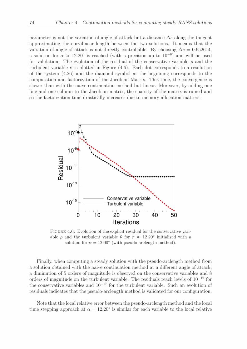
74 Chapter 4. Continuation methods for computing steady RANS solutions
parameter is not the variation of angle of attack but a distance Δs along the tangentapproximating the curvilinear length between the two solutions. It means that thevariation of angle of attack is not directly controllable. By choosing Δs = 0.652614,a solution for α ≈ 12.20◦ is reached (with a precision up to 10−6) and will be usedfor validation. The evolution of the residual of the conservative variable ρ and theturbulent variable ν is plotted in Figure (4.6). Each dot corresponds to a resolutionof the system (4.26) and the diamond symbol at the beginning corresponds to thecomputation and factorization of the Jacobian Matrix. This time, the convergence isslower than with the naive continuation method but linear. Moreover, by adding oneline and one column to the Jacobian matrix, the sparsity of the matrix is ruined andso the factorization time drastically increases due to memory allocation matters.
Iterations
Res
idua
l
0 10 20 30 40 50
10-15
10-13
10-11
10-9
10-7
Conservative variableTurbulent variable
Figure 4.6: Evolution of the explicit residual for the conservative vari-able ρ and the turbulent variable ν for α ≈ 12.20◦ initialized with a
solution for α = 12.00◦ (with pseudo-arclength method).
Finally, when computing a steady solution with the pseudo-arclength method froma solution obtained with the naive continuation method at a different angle of attack,a diminution of 5 orders of magnitude is observed on the conservative variables and 8orders of magnitude on the turbulent variable. The residuals reach levels of 10−12 forthe conservative variables and 10−17 for the turbulent variable. Such an evolution ofresiduals indicates that the pseudo-arclength method is validated for our configuration.
Note that the local relative error between the pseudo-arclength method and the localtime stepping approach at α = 12.20◦ is similar for each variable to the local relative

4.3. Validation and comparison with local time stepping solutions 75
error depicted in the comparison of the naive continuation method and the local timestepping approach at α = 12.00◦ and the reasons of such an error are similar.
4.3.3 Summary
Table 4.1 shows the values of the lift and drag coefficients obtained for steady solutionscomputed at α = 12.20◦ with four different methods: a local time stepping approachwith the recommended cutoffs on the turbulent variable active, a local time steppingapproach with no cutoffs on the turbulent variable (but still some inner cutoffs ac-tive during the computation of the turbulent variable), a naive continuation methodapproach and a pseudo-arclength approach. First, one can observe how the naive con-tinuation method and the pseudo-arclength give similar results. Second, by comparingthe results obtained with the two continuation methods with the result obtained withthe local time stepping approach with all the recommended cutoffs on the turbulentvariable active, one can observe a slight difference of lift and drag coefficients. However,the difference between the two steady solutions (already presented in the left picturesof Figure (4.4)) results in an extremely small error on the aerodynamic coefficients(< 1%). Nevertheless, by removing the cutoffs on the turbulent variable, this error onthe aerodynamic coefficients decreases by 4 orders of magnitude.
Method CL CD
Local time stepping with recommended cutoff 1.237283 0.013172Local time stepping without cutoff 1.247874 0.012333
Naive continuation method 1.247872 0.012332Pseudo-arclength 1.247872 0.012332
Table 4.1: Comparison of the aerodynamic coefficients CL and CD forα = 12.20◦ regarding the computational method used.


77
Chapter 5
The OA209 airfoil in stallconfiguration: linear stability analysisof steady RANS solutions
Contents5.1 Steady RANS solutions of the flow around an OA209 airfoil 78
5.1.1 General overview of the solutions . . . . . . . . . . . . . . . . 78
5.1.2 Solutions close to the stall angle . . . . . . . . . . . . . . . . 82
5.2 Linear global stability analysis of the steady RANS solutions 83
5.2.1 Formalism and tools . . . . . . . . . . . . . . . . . . . . . . . 83
5.2.2 General overview of the stability results . . . . . . . . . . . . 84
5.2.3 Eigenspectra . . . . . . . . . . . . . . . . . . . . . . . . . . . 85
5.2.4 Structure of the mode and influence on the dynamics . . . . . 87
5.2.5 Adjoint mode, wavemaker and local contribution of the flow . 92
5.3 The complex behavior of the stall eigenmode along thepolar curve . . . . . . . . . . . . . . . . . . . . . . . . . . . . 97
5.3.1 From Hopf bifurcations to saddle-node bifurcations . . . . . . 98
5.3.2 Evolution of the angular frequency and growth rate of themode along the curve of steady solutions . . . . . . . . . . . . 100
5.4 Conclusion . . . . . . . . . . . . . . . . . . . . . . . . . . . . . 101
The turbulent flow around a two dimensional OA 209 airfoil in a retreating blade con-figuration (M = 0.16 and Re = 1.8 × 10⁶) is considered. This configuration is similarto that studied in chapter 3 and the mesh used is the same as the one introduced insection 3.1. The study is still performed in the RANS formalism (see chapter 2 for moredetails) with the Spalart–Allmaras turbulence model [151] (also described in chapter2) under the assumption of a fully turbulent flow (i.e. no transition model). However,in this chapter, the steady solutions of the Navier–Stokes equations are obtained fordifferent angles of attack (from α = 12.00◦ to α = 22.00◦) with continuation methods: naive continuation and pseudo arc-length methods (which are introduced in detail

78 Chapter 5. The OA209 airfoil in stall configuration: linear stability analysis ofsteady RANS solutions
in chapter 4) instead of time stepping methods presented in chapter 2 and applied onthis configuration in chapter 3. Such an approach should allow us to reach solutionsthat are unaccessible with local time stepping approach and reduces the total compu-tational time. More precisely, a branch of steady solutions linking the upper and lowerbranches identified in chapter 3 is sought, similarly to the work of Wales and Gaitonde[166].
Next, a stability analysis is performed for each steady solution obtained for differentvalues of α. First, the formalism of the stability analysis is introduced. Then, the twounstable modes observed are introduced : one is a low frequency mode appearing closeto stall and the other is a classic bluff-body vortex shedding mode, which appearsfor higher values of angles of attack and oscillates at a higher frequency. Finally, thecomplex behavior of the low frequency mode along the steady solution is describedclose to stall.
5.1 Steady RANS solutions of the flow around anOA209 airfoil
5.1.1 General overview of the solutions
The vector Q = (ρ, ρu, ρv, ρE, ρν)T is introduced as the steady solution of the Navier–Stokes equations R(Q) = 0. The conservative variables are : the density ρ, thestreamwise velocity along the horizontal axis (x) u, the cross-stream velocity along thevertical axis (y) v and the internal energy E. The vector is completed by the turbulentvariable ν of the Spalart–Allmaras model.
Figure (5.1) shows the ρu field (left) and the ρν field (right) for different angles ofattack. On each picture, the limit of the recirculation bubble, if it exists, is plottedin black. For each case, the position of the corresponding angle of attack is indicatedwith a red dot in the middle picture showing the evolution of the lift coefficient asa function of the angle of attack. This curve is presented and discussed in more de-tail in Figure (5.2). The first angle of attack investigated in pictures (a) and (b) isα = 12.00◦. For this value of α, the flow is fully attached and there is no recirculationbubble. The wake is relatively thin and the level of turbulence in it is extremely low.The second case, α = 16.00◦, depicted in pictures (c) and (d), exhibits the appearanceof a tiny recirculation bubble on the trailing edge. The thickness of the wake, the levelof turbulence as well as the lift coefficient increase with the angle of attack. The nextconfiguration, α = 17.50◦, presented in pictures (e) and (f), corresponds to a maxi-mum value of lift coefficient. The separation point of the recirculation bubble movesbackward, in the direction of the leading edge, resulting in an increase of the recircula-tion bubble size and the thickness of the wake. Pictures (g) and (h) present the fieldsfor α = 18.45◦ just before a sudden drop of lift. The separation point keeps movingtowards the leading edge and the recirculation bubble size as well as the thickness ofthe wake increases. The same angle of attack α = 18.45◦ is presented in pictures (i) and(j) but the flow topology is completely different : the flow is now massively separated,resulting in a much bigger recirculation bubble and wake thickness as well as a larger

5.1. Steady RANS solutions of the flow around an OA209 airfoil 79
α (°)
CL
12 14 16 18 20 22
1
1.2
1.4
1.6
α (°)
CL
12 14 16 18 20 22
1
1.2
1.4
1.6
α (°)
CL
12 14 16 18 20 22
1
1.2
1.4
1.6
α (°)
CL
12 14 16 18 20 22
1
1.2
1.4
1.6
α (°)
CL
12 14 16 18 20 22
1
1.2
1.4
1.6
α (°)
CL
12 14 16 18 20 22
1
1.2
1.4
1.6
α (°)
CL
12 14 16 18 20 22
1
1.2
1.4
1.6
(a) (b)
(c) (d)
(e) (f )
(g) (h)
(i) (j)
(k) (l)
(m) (n)
Figure 5.1: Flow topology for different angles of attack: (a) and (b):α = 12.00◦. (c) and (d): α = 16.00◦. (e) and (f): α = 17.50◦. (g) and(h): α = 18.45◦ on the upper branch. (i) and (j): α = 18.45◦ on thelower branch. (k) and (l): α = 19.00◦. (m) and (n): α = 22.00◦. Leftpictures: ρu field. Middle pictures: position of the steady solution in the
(α,CL) plane. Right pictures: ρν field.
turbulence level in the wake. Also, a second small recirculation bubble appears at thetrailing edge. The coexistence of these solutions was introduced in chapter 3 and anew interpretation, made possible with the use of continuation methods, is presented

80 Chapter 5. The OA209 airfoil in stall configuration: linear stability analysis ofsteady RANS solutions
in detail afterwards in subsection 5.1.2. Then, the case α = 19.00◦ is presented inpictures (k) and (l). The evolution of the recirculation bubble and the wake is similarto the one observed so far. Moreover, the small recirculation at the trailing edge alsogrows and, by doing so, pushes the reattachment point of the large recirculation bubbletowards the leading edge. Finally, the highest angle of attack investigated, α = 22.00◦,is presented in pictures (m) and (n). The flow is now massively separated from almostthe leading edge and the turbulence level is high.
From all these solutions, it is possible to extract several interesting variables thatcan be plotted as a function of the angle of attack and provide a quantitative evolu-tion of the flow. Figure (5.2) shows the evolution of the lift coefficient (a), the dragcoefficient (b), the pitching moment coefficient (c) and the evolution of the separationand reattachment points (respectively in full and dashed black lines) to evaluate therecirculation bubble position (d). The curves showing the evolution of the aerodynamiccoefficient (introduced in appendix A) were presented in chapter 3 for steady solutionscomputed with a local time stepping approach: a discontinuity and the coexistence ofseveral solutions for the same angle of attack was identified. This area is indicatedon the curves (a), (b), (c) and (d) by a grey area. In the present case, which exhibitssolutions obtained with continuation methods, the major difference comes from thecontinuity of all the quantities plotted as a function of the angle of attack, highlightingthe fact that steady solutions that could not be found with a local time stepping ap-proach exist and were successfully identified with the pseudo-arclength method. Apartfrom this difference, the remaining portions of the different curves are similar. One canfirst observe a linear increase of the lift, drag and pitching moment coefficients for thelowest values of angles of attack (from α = 12.00◦ to α = 17.50◦ approximately). Then,stall occurs, characterized by a sudden drop of lift and pitching moment coefficientsand a sudden increase of the drag coefficient. Finally, the lift and pitching momentcoefficients keep decreasing more slowly after stall occurred while the drag coefficientkeeps increasing. As mentioned in the description of Figure (5.1), the separation pointmoves from the trailing to the leading edge as the angle of attack increases. The exactposition of this point is plotted as a function of the angle of attack with a full blackline in picture (d). The position is defined as a fraction of the chord of the airfoil x
c: 1
corresponds to the trailing edge and 0 corresponds to the leading edge. For the lowestangles of attack investigated (α < 13.00◦), the flow is entirely attached. Then, a flowseparation appears at the trailing edge, initiating a recirculation bubble, and slowlymoves towards the leading edge, expanding the size of this recirculation bubble, whichgrows faster as the angle of attack is getting closer to the stall area. Before the stallarea, the flow never reattaches on the airfoil. However, just before the drop of lift, theflow starts reattaching on the airfoil. The evolution of the position of the reattachmentpoint is plotted with a dashed black line in picture (d). Similarly to the separationpoint, the reattachment point is also moving towards the leading edge. Note that as thereattachment point moves backward, the size of the second small recirculation bubbleidentified in Figure (5.1) increases.
To summarize, the phenomena revealed by this analysis are similar to those de-scribed in chapter 3, which validates the use of continuation methods in this configu-ration. A more detailed comparison of the steady solutions obtained with continuation

5.1. Steady RANS solutions of the flow around an OA209 airfoil 81
% o
f cho
rd
12 14 16 18 20
20
40
60
80
100
α (°)22
SEPARATED
α (°)
CM
12 14 16 18 20 22
-0.8
-0.4
0
α (°)
CD
12 14 16 18 20
0.1
0.2
22α (°)
CL
12 14 16 18 20 22
1
1.2
1.4
1.6
(a)
(c)
(b)
(d)
Figure 5.2: Evolution of several quantities related to the flow topologyof steady solutions as a function of the angle of incidence. (a) Evolutionof the lift coefficient. (b) Evolution of the drag coefficient. (c) Evolutionof the pitching moment coefficient. (d) Evolution of the separation (fullblack line) and reattachment points (dashed black line) and identification
of the separated flow area (hatched region).
methods and with a local time stepping approach is presented in appendix C. The stallmechanism identified is a trailing edge stall characterized by a separation point movingfrom the trailing edge to the leading edge as the angle of attack increases. The ques-tion of the validity of such a stall type for these particular airfoil and configuration isaddressed in section 3.2.4. A second small recirculation bubble at the trailing edge forhigh angles of attack is also identified. The coexistence of several solutions for the sameangle of attack is highlighted close to the stall angle similarly to what was observed inchapter 3. However, with the data previously available, stall was associated with anabrupt change of flow topology from the so called upper branch (of high lift) to theso called lower branch (of low lift). With this new approach, it appears that there isactually no discontinuity from one branch to the other as highlighted by the evolutionof the aerodynamic coefficients as well the evolution of the recirculation bubble. The

82 Chapter 5. The OA209 airfoil in stall configuration: linear stability analysis ofsteady RANS solutions
branch that links the upper and lower branches, is named the middle branch. Thisbranch was unaccessible with the classic local time stepping approach but the pseudoarclength method made it possible and, in the end, a result similar to the one of Walesand Gaitonde [166] on a NACA0012 at high Reynolds number is obtained. The nextsection is dedicated to a more detailed description of this zone of coexisting solutions.
5.1.2 Solutions close to the stall angle
CL
18.4 18.45 18.51.2
1.3
1.4
1.5
α(°)
b
d
c
(c)
(d)
(b)
a)
(a)
Figure 5.3: Visualisation of three steady solutions coexisting for a sameangle of attack (α = 18.45◦). (a) Lift coefficient polar curve zoomedin close to stall. The black vertical line refers to the angle of attackconsidered. The three different solutions existing for this angle of attackare marked by a letter, which refers to a picture on the right. (b) Upperbranch solution. (c) Middle branch solution. (d) lower branch solution.
Now that the continuity of the steady solutions have been demonstrated, it is inter-esting to focus on the stall area where several solutions coexist. Figure (5.3) shows, onthe left, the evolution of the lift coefficient in this area. One can observe how the upperbranch, of high lift values, ends in with a saddle-node point (marked by the furthestright black dot). This point also marks the first extremity of the middle branch. Theother extremity of the middle branch corresponds to the second saddle-node bifurca-tion that ends the lower branch (marked by the furthest black dot). In chapter 3, thisstall area is characterized by two steady solutions coexisting for a same angle of attack.With the identification of the middle branch, we acknowledge that there are actuallythree solutions coexisting for each angle of attack in this area. The three pictures onthe right of Figure (5.3) illustrate the topologies of these three different steady solutionsfor the particular value α = 18.45◦ (marked by a vertical line on the polar curve). Eachflow topology is referenced on the polar curve by the corresponding letter : picture (b)corresponds to the high lift solution on the upper branch, picture (c) corresponds tothe solution on the middle branch and picture (d) corresponds to the low lift solutionon the lower branch. One can observe three different flow topologies for each solution

5.2. Linear global stability analysis of the steady RANS solutions 83
: (b) exhibits a medium size recirculation bubble, (c) a larger recirculation bubble and(d) and even larger one coupled with the appearance of a second smaller recirculationbubble at the trailing edge.
5.2 Linear global stability analysis of the steady RANSsolutions
The steady solutions for several angles of attack between α = 12.00◦ and α = 22.00◦
have been computed with continuation methods. Such a range of values allowed us toidentify stall and static hysteresis and a perfect continuity of the steady solutions evenat stall. The objective is to perform a linear stability analysis of each steady solutionin order to see if self-sustained global instabilities can be found for particular anglesof attack. Particularly, the identification of a mechanism that could be directly linkedto stall will be carefully investigated. First, the formalism of the linear global stabilityanalysis is introduced: particularly, it is shown how this linear study can be written asan eigenvalue problem where the eigenvalue characterizes the temporal behavior of theinstability and the eigenmode corresponds to the spatial structure of the instability.Afterwards, the results obtained for the linear stability analysis of the steady solutionscomputed in section 5.1 are presented. Several tools, used to identify the regions ofthe flow that could be at the origin of the mechanisms identified, are also introduced.
5.2.1 Formalism and tools
The governing equations of the system are the compressible Navier–Stokes equations(defined by (2.17) in chapter 2) closed with a turbulence model in the RANS framework.In the present case, the Spalart–Allmaras turbulence model, defined in (2.23), is chosen.The flow variable q = (ρ, ρu, ρv, ρE, ρν)T satisfies these governing equations, which,after spatial discretization with a finite volume method, can be formally written:
dq
dt= R(q) (5.1)
where the vector q refers to variables of the system : q = (ρ, ρu, ρv, ρE, ρν)T . A firstassumption is made on the form of the solution of the Navier–Stokes equations : theycan be written as the sum of a steady solution Q and time dependent perturbation q′
of small amplitude ε :
q = Q+ εq′ (5.2)
where Q satisfies :
R(Q) = 0 (5.3)
By replacing decomposition (5.2) into (5.3) and linearizing the equations, the systemcan be written as :

84 Chapter 5. The OA209 airfoil in stall configuration: linear stability analysis ofsteady RANS solutions
dq′
dt= J (Q)q′ (5.4)
where J (Q) is the Jacobian of the system R evaluated at Q. Details about thecomputation of this matrix is given in section 4.2.1 of chapter 4. Moreover, the timedependent perturbations are sought under the form of normal modes:
q′ = qeλt (5.5)
where q designates the spatial behavior of the mode and λ = σ + iω its temporalbehavior (σ its growth rate and ω its angular frequency). A base flow Q is consideredasymptotically stable if the perturbation tends to zero for large times, which meansσ < 0 for all modes found. Otherwise, if σ > 0, a mode is considered asymptoticallyunstable. The base flow is considered unstable if at least one mode is unstable .Finally, equation (5.4) can be written as an eigenvalue problem where (λ, q) is theeigenvalue/eigenvector combination which verifies:
J (Q)q = λq (5.6)
where q = (ρ, ρu, ρv, ρE, ρν)T .
The computation of the eigenspectrum is performed using Krylov methods with ashiff-and-invert strategy [143] available in the open source library ARPACK [130]. Thedirect parallel LU solver MUMPS [120] is used as linear solver. As already mentionedin section 4.2.2, the LU factorization is costly and has high memory requirements.However, in our two dimensional case this is not a limitation. The tools used in thepresent work to compute the Jacobian matrix and the eigenvalue/eigenvector combi-nation have been validated first by Mettot et al. [108] in the case of a two dimensionaldeep cavity with several turbulence models and numerical schemes and used in severalstudies afterwards (see for instance Beneddine et al. [13], Bonne et al. [17] or Paladiniet al. [123]).
5.2.2 General overview of the stability results
Figure (5.4) exhibits the evolution of the lift coefficient as a function of the angle ofattack already presented in Figure (5.2). The dashed portions of the curve correspondto the solutions for which an unstable eigenvalue is found (i.e. an eigenvalue λ witha positive growth rate σ). One can observe two very distinct zones with an unstablemode : a first one close to the stall area (α ≈ 18.45◦) and a second one for high anglesof attack (α > 20.50◦) when the flow is completely detached. It appears that, foreach area, it is possible to identify a coherent evolution of the eigenvalue and a similarstructure of the eigenmodes for the different angles of attack. However, the angularfrequency ω (imaginary part of the eigenvalue λ) and the structure of the modes aredrastically different between the two zones. From this point, the mode identified closeto the stall angle will be designated as the stall mode. The other one, appearing whenthe flow is massively separated, is actually a bluff body vortex shedding mode as will

5.2. Linear global stability analysis of the steady RANS solutions 85
be shown in the rest of this chapter.
CL
12 16 20
1
1.2
1.4
1.6
α(°)
Stall
mode
Vortex
shedding
mode
Figure 5.4: Lift coefficient curve and associated linear stability state.The angles of attack for which the linear stability analysis of the steadysolutions reveals an unstable mode are plotted with a dashed black line.Otherwise, a full black line is used. Two different zones of interest areidentified : one close to stall and one for high angles of attack, for which
the flow is massively separated.
5.2.3 Eigenspectra
Figure (5.5) shows the unstable eigenvalues identified for a particular angle of attack ineach area : (a) presents the results obtained for α = 18.49◦ on the upper branch (closeto stall) and (b) presents the results obtained for α = 21.00◦ on the lower branch (whenthe flow is massively separated). The modes are marked by red dots in the complexplane (σ, ω). Note that there are actually two red dots in each figure : one correspondsto the actual mode and the other to its complex conjugate of similar growth rate andopposite angular frequency. The grey areas highlight the zones where the modes areunstable (σ > 0) and note that the red dots are in these areas.
The main difference between the two pairs of eigenvalues comes from the order ofmagnitude of their angular frequency ω : for the unstable mode identified close to stallfor α = 18.49◦, ω = 0.0086 (picture (a)) while for the unstable mode identified athigher angles of attack for α = 21.00◦, ω = 0.515 (picture (b)). This means that thefrequency of the phenomenon identified close to stall is two orders of magnitude lowerthan the bluff body vortex shedding phenomenon. A more common way to quantifyunsteady phenomena occurring around airfoils is to consider the Strouhal number baseon the chord length weighted by the sine of the angle of attack :

86 Chapter 5. The OA209 airfoil in stall configuration: linear stability analysis ofsteady RANS solutions
σ
ω
-0.02 -0.01 0 0.01-0.02
-0.01
0
0.01
0.02
σ
ω
-0.02 -0.01 0 0.01-1
-0.5
0
0.5
1
(a) (b)
Figure 5.5: Visualisation of two eigenspectra for two different angles ofattack. (a) Stall mode for α = 18.49◦ on the upper branch, just beforestall. (b) Vortex-shedding mode for α = 21.00◦ on the lower branch,when the flow is massively separated. For each spectrum, the leading
mode and its associated complex conjugate are represented.
St =ω · c · sin(α)2π · U∞
(5.7)
With ω the angular frequency, c the chord of the airfoil, α the angle of attack andU∞ the far field velocity in the x direction (U∞ = 0.16 in our case). The correspondingvalues of Strouhal number are summarized in Table 5.1. The vortex shedding modehas a very classic Strouhal number St ≈ 0.2, similar to what is usually found in the lit-erature (see for instance [142]). The Strouhal number of the stall mode, St = 0.00271,is two orders of magnitude lower than the Strouhal number of the bluff body vortexshedding mode, which echoes the value found for low frequency oscillations, which ap-pear close to stall (detailed in section 1.3.2).
Mode α (◦) σ ω StStall 18.49 6.56× 10⁻⁴ 8.60× 10⁻³ 0.0027
Vortex shedding 21.00 6.2× 10⁻³ 5.73× 10⁻¹ 0.20
Table 5.1: Components of the eigenvalues for two different types ofmode : stall (α = 18.49◦)and vortex shedding (α = 22.00◦ modes.Growth rate σ, angular frequency ω and associated Strouhal numberSt scaled on the chord length weighted by the sine of the angle of attack.

5.2. Linear global stability analysis of the steady RANS solutions 87
5.2.4 Structure of the mode and influence on the dynamics
Very different orders of magnitude are identified between the angular frequencies of thetwo pairs of eigenvalues. It is now interesting to examine the respective structures ofthe associated eigenmodes. First, the structures of the modes are introduced and thenthe influence on their respective baseflows is presented.
5.2.4.1 Eigenmodes
Figure (5.6) presents the real part of the eigenmodes. Pictures (a) and (c) describethe stall mode (α = 18.49◦) and pictures (b) and (d) present the vortex shedding mode(α = 21.00◦). The upper ones correspond to the streamwise velocity ρu componentof the modes and the lower ones to the turbulent variable ρν. On each picture, therecirculation bubble obtained from the associated steady solution is represented by ablack line.
(a) (b)
(c) (d)
Figure 5.6: Visualisation of the structure of the eigenmodes. (a) Realpart of the ρu field of the stall eigenmode (α = 18.49◦). (c) Real partof the ρν field of the stall eigenmode (α = 18.49◦). (b) Real part of theρu field of the vortex-shedding eigenmode (α = 21.00◦). (d) Real part
of the ρν field of the vortex-shedding eigenmode (α = 21.00◦).
The spatial pattern of the streamwise velocity ρu of the stall mode, presented inFigure (5.6)(a), shows a large pulsating structure starting on the suction edge of theairfoil just before the separation point of the steady solution. The structure extendsuntil the end of the recirculation bubble of the steady solution. The turbulent variableρν exhibits similar pulsating structures but also exists in the wake of the steady solu-tion, downstream from the recirculation region (picture (c)). The amplitude reaches itspeak in the upper part of the wake, close to the recirculation region. The shape of thismode is very similar to the one observed around a NACA 0012 at Reynolds numberRe = 6.0× 10⁶ and Mach number M = 0.15 by Iorio [76] presented in Figure 1.10.
The spatial pattern of the streamwise velocity shown in Figure (5.6)(b) is typical ofa vortex-shedding eigenmode: two rows of large structure patterns which oscillate out

88 Chapter 5. The OA209 airfoil in stall configuration: linear stability analysis ofsteady RANS solutions
of phase in the streamwise direction and located in the wake of the flow. The struc-tures reach their largest amplitude downstream from the recirculation region of thesteady solution and slowly vanish in the far field. The turbulent variable ρν depictedin Figure (5.6)(d) shows the same kind of structures in the streamwise direction andlocated downstream from the airfoil although more affected by the wake of the steadysolution, whose boundaries are clearly visible on this component.
5.2.4.2 Superimposition of the eigenmodes and the steady solutions
Once the structures of the eigenmodes are well known and understood, it is interestingto observe how these modes could affect the steady solution. A first order approxi-mation of the unsteady solution of the Navier–Stokes equations can be obtained bysumming the steady solution Q and the small time dependent perturbation q′ (see sec-tion 5.2.1 for more details). Equation (5.8) details the expression of the approximatedsolution with ε a small amplitude perturbation, q the eigenmode, σ the growth rate ofthe mode and ω the angular frequency of the mode.
qapprox = Q+ 2εeσt[qr cos(ωt)− qi sin(ωt)] (5.8)
Many of those variables are known from the stability analysis. However, the ampli-tude of the perturbation ε remains unknown. The exact determination of this variablein our approach is complicated and would require time-consumming computations. In-deed, as demonstrated by Sipp and Lebedev [149] in the case of the flow past a cylinderat low Reynolds number, an equation for the amplitude might be obtained by originallyconsidering a higher order of approximation of the Navier–Stokes equations: such asq = Q + εq′ + ε2q′′ + .... The resolution of this amplitude equation would give us theparameter ε. Then, it would be necessary to wait for the phenomenon to slowly be am-plified based on the exponential evolution of the growth rate eσt until the phenomenonwould become significant. However, even in that case, the solution computed wouldstill be a first order approximation and it would require to investigate the amplitudesof higher order perturbations to obtain the exact solution. In order to avoid such acomplexity, we just set an arbitrary amplitude A such that A = 2εeσt. We set thevalue of A to ensure that significant changes of the base flow can be observed. Such anapproach, although quantitatively approximate, provides a useful qualitative overviewof the global dynamics of the instabilities and of how the modes affect the baseflow.The values of A used in our cases are referenced in Table 5.2.
Stall mode Vortex Shedding modeA 10 20
Table 5.2: Values of the amplitude chosen to compute the approximateunsteady solution qapprox.
Figure (5.7) presents the approximated solution qapprox over a period T = 2πω
(withω the angular frequency of the mode) for the stall mode at α = 18.49◦. One can

5.2. Linear global stability analysis of the steady RANS solutions 89
t
CL
0 200 400 600
1.3
1.4
1.5
1.6
1.7
t
CL
0 200 400 600
1.3
1.4
1.5
1.6
1.7
t
CL
0 200 400 600
1.3
1.4
1.5
1.6
1.7
t
CL
0 200 400 600
1.3
1.4
1.5
1.6
1.7
t
CL
0 200 400 600
1.3
1.4
1.5
1.6
1.7
t
CL
0 200 400 600
1.3
1.4
1.5
1.6
1.7
(a) (b)
(c) (d)
(e) (f )
(g) (h)
(i) (j)
(k) (l)
Figure 5.7: Visualisation of the effect of the stall eigenmode on thesteady solution for α = 18.49◦ for an arbitrary amplitude B = 10. Leftpictures: ρu field. Middle pictures: position of the solution in the (t, CL)plane. Right pictures: ρν field. Six different times are considered over aperiod T . (a) and (b): t = 0. (c) and (d): t = T
6 . (e) and (f): t = T3 .
(g) and (h): t = T2 . (i) and (j): t = 2T
3 . (k) and (l): t = 5T6 .
observe the perfect sinusoidal form of the evolution of the lift coefficient over a period.The solution at t = 0 (pictures (a) and (b)) corresponds to a minimum of lift valueover the period. It exhibits two recirculation bubbles: a large one on the suction sideof the airfoil and a smaller one located at the trailing edge. The wake is wide andthe turbulent level in it is high. The solution at t = T
6(pictures (c) and (d)), which
corresponds to an increase of lift value, presents a displacement of the separation pointtowards the trailing edge resulting in a smaller recirculation bubble on the suctionside of the airfoil. The smaller recirculation bubble located at the trailing edge of the

90 Chapter 5. The OA209 airfoil in stall configuration: linear stability analysis ofsteady RANS solutions
airfoil no longer exists and the wake is thinner with a lower turbulence level in it. Theseparation point keeps moving towards the trailing edge as the lift coefficient increasesas shown in the solution at t = T
3(pictures (e) and (f)). One can observe a region
of higher speed in the streamwise direction just above the recirculation bubble and aregion of negative ν in the upper part of the wake, which is even thiner than previously.The solutions at t = T
2(pictures (g) and (h)) correspond to a maximum of lift value
over the period. The topology of the flow is very similar to that observed at t = T2: no
visible differences in the size of the recirculation bubble or the thickness of the wake.The main difference comes from an even higher speed above the recirculation bubbleand even smaller values of ν. Afterwards, for t = 2T
3(pictures (i) and (j)) the lift
value starts decreasing. It is characterized on the flow topology by a displacement ofthe separation point towards the leading edge resulting in an increase of the recircula-tion bubble size and of the thickness of the airfoil. One can also observe that the twosolutions at t = T
3and t = 2T
3exhibit similar lift coefficient values but very different
topologies (this difference is also observed between the solutions at t = T6
and t = 5T6
depicted in pictures (k) and (l)). Indeed, the second one exhibits a larger recirculationzone on the suction side of the airfoil and also a second recirculation bubble located atthe trailing edge with a thicker wake. More generally, one can observe that the stallmode, whose structure is located just above the recirculation bubble, tends to affectthe size of this recirculation bubble. Therefore, the approximated solution pulsatesbetween a high lift state with a tiny recirculation bubble located at the trailing edgeand a low lift state with a very large recirculation bubble on almost all the suction sideof the airfoil : stalled and unstalled position are alternatively encountered.
A similar approach is used for the vortex shedding mode and depicted in Figure(5.8). The solution at t = 0 (pictures (a) and (b)) corresponds to a maximum of lift overthe period. It exhibits two rows of a pattern, which oscillates out of phase (similarlyto the structure of the vortex shedding eigenmode). This pattern is identified at anytime over the period, and the differences between the flow topologies can be identifiedby looking at the recirculation bubbles. Three different ones exist at t = 0: a large onelocated on the suction side of the airfoil, a tiny one at the trailing edge (under the largeone) and a third one in upstream in the wake. At t = T
6(pictures (c) and (d)), the
large one is convected upstream, going over the tiny one that slightly increases while theone already in the wake is convected even more upstream. These displacements of therecirculation bubbles are characterized by a drop of lift. The same tendency is observedat t = T
3(pictures (e) and (f)) with two shrinking bubbles convected upstream in the
wake and one becoming bigger at the trailing edge of the airfoil. At t = T2
(pictures (g)and (h)), corresponding to a minimum value of lift over the period, the most upstreamrecirculation bubble has vanished while the one at the trailing edge is bigger and a newone, of approximately the same size, is appearing above the airfoil. Afterwards, thelift coefficient is increasing again (pictures (i) and (j) corresponding to t = 2T
3) as the
recirculation bubble above the airfoil becomes a large recirculation bubble covering thewhole suction side of the airfoil. The other one, located at the trailing edge, is pushedupstream by the size increase of the large one. The same tendency is observed for thelast time depicted t = 5T
6at which the recirculation bubble on the suction side of the
airfoil is even larger while the other one is convected even more upstream. Afterwards,the same behavior is repeated from t = 0 with the appearance of a tiny recirculation

5.2. Linear global stability analysis of the steady RANS solutions 91
CL
0 2 4 6 8 10 12
0.84
0.88
0.92
0.96
CL
0 2 4 6 8 10 12
0.84
0.88
0.92
0.96
t
t
CL
0 2 4 6 8 10 12
0.84
0.88
0.92
0.96
t
CL
0 2 4 6 8 10 12
0.84
0.88
0.92
0.96
t
CL
0 2 4 6 8 10 12
0.84
0.88
0.92
0.96
t
CL
0 2 4 6 8 10 12
0.84
0.88
0.92
0.96
t
(a) (b)
(c) (d)
(e) (f )
(g) (h)
(i) (j)
(k) (l)
Figure 5.8: Visualisation of the effect of the vortex-shedding eigenmodeon the steady solution for α = 21.00◦ for an arbitrary amplitude B = 20.Left pictures: ρu field. Middle pictures: position of the solution in the(t, CL) plane. Right pictures: ρν field. Six different times are consideredover a period T . (a) and (b): t = 0. (c) and (d): t = T
6 . (e) and (f):t = T
3 . (g) and (h): t = T2 . (i) and (j): t = 2T
3 . (k) and (l): t = 5T6 .
bubble under the large one and so on. More generally, one can observe recirculationbubbles convected upstream one after the other: the large one on the suction side ofthe airfoil and the smaller one located at the trailing edge of the airfoil. It resultsin two out of phase rows of an oscillating pattern, which generate an oscillating wakesimilar to a Von Karman street [83] [84].

92 Chapter 5. The OA209 airfoil in stall configuration: linear stability analysis ofsteady RANS solutions
5.2.5 Adjoint mode, wavemaker and local contribution of theflow
The global stability analysis of the steady solutions revealed the appearance of linearlyunstable mechanisms for some values of α. However, although this method gives goodinsight into the structure, frequency and linear growth of the instability, it does notprovide any information about the region of the flow where the instability develops.The concept of wavemaker was introduced by Huerre and Monkewitz [73] to locate thisregion. They defined it as the region where instability waves are intrinsically generatedin globally unstable flows. Extending the work of Hill [66], Giannetti and Luchini [59]proposed an alternative approach to define the concept of wavemaker. Their approachrelies on the concept of structural sensitivity, which characterizes the effects of local-ized changes of the flow operator on the eigenvalues. This led to the most commonlyaccepted definition of the wavemaker: the region of maximum structural sensitivity.Hill [66] and Giannetti and Luchini [59] all used it in the case of the flow behind acylinder, in order to identify the regions where a control cylinder be the most effective.Since then, this approach has been used in many studies to identify the regions of theflow where the self-sustained mechanism induces the largest eigenvalue variation (seefor instance [96] [106] or [123]). Note that the definitions introduced by Huerre andMonkewitz [73] and Giannetti and Luchini [59] are for different frameworks: respec-tively local and global stability analysis frameworks. However, Juniper and Pier [82]proved that the definition of Giannetti and Luchini [59] can be extended in the caseof local stability analysis with decent results as long as a weakly nonparallel flow isconsidered. In the spirit of the wavemaker, Paladini et al. [123] proposed an alternativeapproach based on the decomposition instead of a variation of the linear operator. Inan attempt to identify the regions of the flow which contribute the most to the growthrate and the frequency respectively Marquet and Lesshafft [95] proposed a proportionalmodification of the operator, still based on the concept of sensitivity, which is furtherdescribed and used in the work of Paladini et al. [123]1. This approach, named localcontribution, offers the advantage of identifying if the regions of the flow contributepositively or negatively to the linear growth rate and angular frequency of the eigen-value.
In this subsection, we intend to apply the sensitivity tools developed by Gianettiand Luchini [59] and Paladini et al. [123] in order to identify the most sensitive regionsof the flow. First, the notion of adjoint mode, which is used in all the aforementionedtools, is introduced. Then, the results obtained with the wavemaker are presented and,finally, the local contribution of the flow to the growth rate and angular frequency isshown.
5.2.5.1 Definition of the adjoint mode
As a reminder, λ is the eigenvalue of the Jacobian matrix J (Q) and q its eigenvector,designated as the direct global mode of the steady solution Q, which are linked through
1A link with the wavemaker function of Giannetti and Luchini [59] as well as a detailed comparisonof the two approaches in the case the flow behind a cylinder can be found in the PhD of Paladini [122]
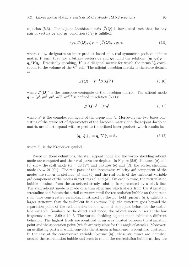
5.2. Linear global stability analysis of the steady RANS solutions 93
equation (5.6). The adjoint Jacobian matrix J (Q) is introduced such that, for anypair of vectors q1 and q2, condition (5.9) is fulfilled:
〈q1,J (Q)q2〉V = 〈J (Q)q1, q2〉V (5.9)
where 〈·, ·〉V designates an inner product based on a real symmetric positive definitematrix V such that two arbitrary vectors q1 and q2 fulfill the relation: 〈q1, q2〉V =q1
∗V q2. Practically speaking, V is a diagonal matrix for which the terms Vk corre-spond to the volume of the kth cell. The adjoint Jacobian matrix is therefore definedas:
J (Q) = V −1J (Q)∗V (5.10)
where J (Q)∗ is the transpose conjugate of the Jacobian matrix. The adjoint modeq† = (ρ†, ρu†, ρv†, ρE†, ρν†)T is defined in relation (5.11):
J (Q)q† = λ∗q† (5.11)
where λ∗ is the complex conjugate of the eigenvalue λ. Moreover, the two bases con-sisting of the entire set of eigenvectors of the Jacobian matrix and the adjoint Jacobianmatrix are bi-orthogonal with respect to the defined inner product, which results in:
〈q†i , qj〉V = q†∗
i V qj = δij (5.12)
where δij is the Kronecker symbol.
Based on these definitions, the stall adjoint mode and the vortex shedding adjointmode are computed and their real parts are depicted in Figure (5.9). Pictures (a) and(c) show the stall mode (α = 18.49◦) and pictures (b) and (d), the vortex sheddingmode (α = 21.00◦). The real parts of the streamwise velocity ρu† component of themodes are shown in pictures (a) and (b) and the real parts of the turbulent variableρν† component of the modes in pictures (c) and (d). On each picture, the recirculationbubble obtained from the associated steady solution is represented by a black line.The stall adjoint mode is made of a thin structure which starts from the stagnationstreamline and follows the airfoil curvature until the recirculation bubble on the suctionside. The conservative variables, illustrated by the ρu† field (picture (a)), exhibits alarger structure than the turbulent field (picture (c)): the structure goes beyond theseparation point of the recirculation bubble while it stops just before for the turbu-lent variable. Similarly to the direct stall mode, the adjoint mode pulses at the lowfrequency ω = −8.60 × 10⁻³. The vortex shedding adjoint mode exhibits a differentbehavior. The highest levels are identified in an area located between the stagnationpoint and the separation point (which are very close for this angle of attack). Moreover,an oscillating pattern, which convects the structures backward, is identified upstream.In the case of the conservative variable (picture (b)), these structures are identifiedaround the recirculation bubble and seem to round the recirculation bubble as they are

94 Chapter 5. The OA209 airfoil in stall configuration: linear stability analysis ofsteady RANS solutions
(a) (b)
(c) (d)
Figure 5.9: Visualisation of the structure of the adjoint modes. (a)Real part of the ρu† field of the stall adjoint mode (α = 18.49◦). (c) Realpart of the ρν† field of the stall adjoint mode (α = 18.49◦). (b) Real partof the ρu† field of the vortex-shedding eigenmode (α = 21.00◦). (d) Real
part of the ρν† field of the vortex-shedding eigenmode (α = 21.00◦).
convected backward. In the end, similarly to the direct modes, the stall adjoint modeis located close to the airfoil while the vortex shedding adjoint mode is propagated inthe freestream.
5.2.5.2 The wavemaker function in the global stability framework
Chomaz [29] noticed for the Ginzburg-Landau equation that the wavemaker can beidentified as the overlapping region between the direct and adjoint modes. This ap-proach was extended to open flows by Giannetti and Luchini [59]. The implementationof this concept in this case is to consider a perturbation of the Jacobian matrix byanother matrix δJ . The form of the matrix is considered such that the perturbationonly affects the kth cell of the mesh, which results in a diagonal block matrix with alldiagonal blocks equal to zero except the one corresponding to the kth cell. In the end,it is shown that, for each cell, the wavemaker function can be written as the productof the p-Euclidian norm of the direct and the adjoint mode:
Wak =||qk|| · ||q†k|| (5.13)
This function quantifies how the eigenvalue responds to a localized forcing of agiven perturbation in the form of an internal forcing. Physically, in this definition, thedirect mode (which propagates downstream from the wavemaker region) indicates theregion of the flow where the perturbation has a significant amplitude and the adjointmode (which propagates upstream) indicates the most receptive region of the flow toa forcing. Consequently, with this definition of the wavemaker, the most sensitive re-gions of the flow are those which simultaneously have a perturbation with a significantamplitude and a significant receptivity to perturbations. Furthermore, according to

5.2. Linear global stability analysis of the steady RANS solutions 95
Giannetti and Luchini, the regions where eigenvalue changes are the strongest alsocorrespond to the regions where the self-sustained dynamics of the flow starts.
(a) (b)
Figure 5.10: Visualisation of the structure of the wavemakers Wa. (a)Based on the direct and adjoint stall modes for α = 18.49◦. (b) Based
on the direct and adjoint vortex shedding modes for α = 21.00◦.
This function is plotted for the two modes in Figure (5.10): picture (a) exhibitsthe result for the stall mode at α = 18.49◦ while picture (b) exhibits the result forthe vortex shedding mode at α = 21.00◦. The structure of the wavemaker for thestall mode stretches from the stagnation point to just before the separation point byfollowing the shape of the airfoil. It seems to be driven by the turbulent variable of theadjoint mode as they exhibit very similar structures as can be observed by comparingFigures (5.9)(c) and (5.10)(a). The structure of the wavemaker for the vortex sheddingmode stretches from the stagnation point to the separation point. The correspondingarea is smaller than the one of the stall mode as the separation point is closer to theleading edge but the intensity in it is higher, particularly close to the separation point.
5.2.5.3 Local contributions of the eigenvalues
The concept of local contribution, introduced by Paladini et al. [123], is also inves-tigated. The aim of this approach is to evaluate how each region contributes to theglobal dynamics of the flow and more particularly to the growth rate and the frequencyof the eigenmode. For the kth cell of the mesh, the density function dk is defined inequation (5.14):
dk =λ(q∗kq
†k) (5.14)
The local contribution of the flow to the growth rate is defined as the real part ofthe density dk: (dk) and the local contribution of the flow to the angular frequencyis defined by the imaginary part of the quantity dk: �(dk). Note that the growth rateσ and the angular frequency ω are linked to the density dk by equations (5.15) and(5.16):
σ =Nc∑k=1
((dk)Vk)
ω =Nc∑k=1
(�(dk)Vk)
(5.15)
(5.16)

96 Chapter 5. The OA209 airfoil in stall configuration: linear stability analysis ofsteady RANS solutions
(a) (b)
Figure 5.11: Visualisation of the sensitivity of the eigenvalue for thestall mode at α = 18.49◦. (a) Influence on the growth rate ((dk)). (b)
Influence on the angular frequency (�(dk)).
Figure (5.11) presents the real and imaginary parts of the density dk for the stallmode: picture (a) exhibits (dk) and picture (b) �(dk). The regions pointed out, cor-responding to the the leading edge and the separation point, are similar to the regionsindicated by the wavemaker function in Figure (5.10)(a) although not exactly the same.The contribution to the growth rate (Figure (5.11)(a)) is only positive, which seems toindicate that there is no region of the flow which stabilizes the dynamics. Particularly,the leading edge region is mainly responsible for the positive value of the growth ratewhile the separation point has a lesser impact on the growth rate. The contributionto the angular frequency (Figure (5.11)(b)) is mostly located on the suction side of theairfoil between the point of maximum thickness of the airfoil and the separation pointwith a high peak just before the separation point. The contribution is mostly posi-tive as only a very small area of relatively low intensity is identified at the leading edge.
(a) (b)
(c) (d)
Figure 5.12: Visualisation of the sensitivity of the eigenvalue for thevortex shedding mode at α = 21.00◦. (a) and (c): influence of the growthrate ((dk)). (b) and (d): influence of the angular frequency (�(dk)).
The case of the vortex shedding mode is depicted in Figure (5.12). Two differentlevels of zoom and saturation are depicted: pictures (a) and (b) show a global view

5.3. The complex behavior of the stall eigenmode along the polar curve 97
of the airfoil with a low saturation level while pictures (c) and (d) exhibit a zoom inclose to the leading edge with a higher saturation level. Pictures (a) and (c) show thecontribution of the flow to the growth rate (dk) while pictures (b) and (d) presentthe contribution of the flow to the angular frequency �(dk). Two main zones of inter-est are identified: one close to the leading edge and the other downstream from therecirculation bubbles. The highest levels are identified close to the leading edge (andpresented in pictures (c) and (d)). One can note that the contributing regions aremore spread for the vortex shedding mode than for the stall mode, which, based onequations (5.15) and (5.16) explains the difference of maximum value of the densities(particularly visible by comparing (dk) for the two modes). Contrary to the stallmode, the regions of the flow differently contribute to the growth (picture (a) and (c)).Particularly, the thin region located at the leading edge between the stagnation pointand the separation point has the highest intensity and a positive contribution whilethe regions of negative contribution are more spread and with a much lower intensity.The imaginary part of the density �(dk) also reveals a spread region of low intensitylocated downstream from the two recirculation bubbles and a more condensed regionof higher intensity. The first region positively contributes to the angular frequency andstrongly recalls the contribution to the angular frequency observed by Paladini et al.in the case of a flow around a cylinder [123]. The second region, on the other hand,strongly recalls the stall mode as can be observed by comparing Figures (5.11)(b) and(5.12)(d): a region at the leading edge with a negative contribution and a region at theseparation point with a positive contribution.
5.2.5.4 Conclusion on the sensitivity analysis of the flow
In the end, the two sensitivity tools (wavemaker Wa and local contribution to theeigenvalue dk) used to identify the zones at the origin of the dynamics observed pro-vide mostly similar results. Although a contributing region located downstream fromthe recirculation bubbles is identified only for the vortex shedding mode, the othercontributing regions are similar for the two modes: the leading edge and the sepa-ration point. This observation raises some questions regarding the results obtained.Indeed, this region is precisely the one which the RANS approach (and particularly theSpalart–Allmaras model) fails to precisely predict. The main reason for this failure isthe fully turbulent approach which prevent the development of a laminar to turbulenttransition and possibly of a laminar separation bubble. The use of another turbulencemodel, possibly coupled to a transition model, would be an interesting path to inves-tigate in future work in order to consolidate those results.
5.3 The complex behavior of the stall eigenmode alongthe polar curve
The stall eigenmode was described for the particular angle of attack α = 18.49◦. Actu-ally, this mode is unstable for other values of α as was shown in Figure (5.4) and canbe tracked along the curve of steady solutions around stall angle even when the modeis stable. Moreover, it appears that, while the structure of the eigenmode is similar

98 Chapter 5. The OA209 airfoil in stall configuration: linear stability analysis ofsteady RANS solutions
for each angle of attack at which it exists, the eigenvalues present a complex behavioralong the curve of steady solutions.
5.3.1 From Hopf bifurcations to saddle-node bifurcations
In this subsection, we intend to describe the complex behavior of the eigenvalues alongthe steady solution curve. An easy way to identify the evolution of this pair of eigen-values is to plot them for different values of α on the same graph. This is the point ofFigure (5.13). The union of pictures (a) and (b) to respectively (c) and (d) correspondsto the entire polar curve and the associated entire superimposed spectra.
Starting with pictures (a) and (b), the stall mode and its complex conjugate arefirst identified for α = 12.00◦ (not represented on the polar curve in picture (a)). Atthis angle of attack the mode is stable (σ ≈ −0.017) and unsteady (ω ≈ 0.024). Thebehavior of the eigenvalue remains almost similar until α ≈ 18.35◦. After this angleof attack, by increasing the curvilinear abscissa, the stall mode becomes less and lessstable and, in the mean time, its angular frequency decreases. Then, at some pointon the upper branch, the stall mode becomes unstable (marked on the polar curve bya switch from full blue line to dashed blue line). Although the mode is now unsta-ble, its angular frequency keeps following the same evolution so that, at some point,it reaches the axis ω = 0. During the whole process, from α = 12.00◦, the complexconjugate mode follows the exact same behavior in mirror symmetry with respect tothe axis ω = 0. This means that the the two unsteady modes merge into a doublesteady eigenvalue. Then, this double eigenvalue splits into two steady eigenvalue. Thisstate corresponds to the pair of eigenvalues plotted with empty red dots and markedby the dashed red lines on the polar curve (tiny area at the end of the upper branch).Afterwards, one unstable eigenvalue tends to become even more unstable (its value ofσ increases) while the other unstable eigenvalue is stabilized. The green dashed lineand the green empty dots correspond to the state where an unstable steady eigenvaluecoexist with a stable steady eigenvalue. The two extrema steady eigenvalues corre-spond to the last point of the middle branch plotted in dashed green line in picture(a). The second part of the polar curve is described in pictures (c) and (d). Notethat the behavior is similar to one depicted in pictures (a) and (b) but backward. Themain difference is that the arc described by the eigenvalues seems to be shifted to theright for the lower branch, which corresponds to a larger range of existence of unstableunsteady modes (blue dashed lines) on the lower branch than on the upper branch.In the end, the stall mode is unstable for a range of angles of attack which seem tocorrespond to the values for which stall occurs and becomes steady at the very end ofthe upper and lower branches and on all the middle branch.
To summarize this behavior and introduce the bifurcations that can be deduced, aschematic representation is proposed in Figure (5.14). The left picture is a schematizedrepresentation of the hysteretic region of the polar curve. The curve is split into sevendifferent areas marked by a different color code and an associated number. Two zonesare labelled 1 and plotted with full blue lines, two others are labelled 2 and plottedwith dashed blue, two others are labelled 3 and plotted with red dashed and the lastone is labelled 4 and plotted with green dashed line. This color code is similar to that

5.3. The complex behavior of the stall eigenmode along the polar curve 99
s
α(°)
CL
18.4 18.44 18.481.2
1.3
1.4
1.5
σ
ω
-0.02 0 0.02
-0.02
0
0.02
s
α(°)
CL
18.4 18.44 18.481.2
1.3
1.4
1.5
σ
ω
-0.02 0 0.02
-0.02
0
0.02
(a) (b)
(c) (d)
Figure 5.13: (a) and (c): lift coefficient polar curves zoomed in closeto stall. The colored parts of the curves highlight the angles of attackfor which the spectrum is represented. (b) and (d): superimposition ofall the eigenspectra of all the angles of attack considered in the complexplane (σ, ω). The arrows associated with the letter s in (a) and (c)indicate the direction of a positive curvilinear abscissa. The arrows in(b) and (d) indicate the evolution of the eigenvalue while moving alongthe curve of steady solutions with an increasing curvilinear abscissa. Thecolor code matches between the left and right pictures. Full blue line orfull blue circle: two unsteady stable modes. Dashed blue line or emptyblue circle : two unsteady unstable modes. Dashed red line or emptyred circle : two steady unstable modes. Dashed green line or greencircle : one unstable steady mode (empty circle) and one stable steadymode (full circle). (a) and (b): from α = 12.00◦ to α = 18.46◦ on themiddle branch. (c) and (d): from α = 18.46◦ on the middle branch to
α = 18.80◦.
used in Figure (5.13) and is related to the behavior of the eigenvalues in this area. De-limiters are present between the areas and refer to particular states of the eigenvalues :

100 Chapter 5. The OA209 airfoil in stall configuration: linear stability analysis ofsteady RANS solutions
CL
α
ω
σ
ω
σ
ω
σ
ω
σ
ω
σ
ω
σ
ω
σ
H
D
SN
SN
D
H
12
3
4
3
21
1
2
3 4
H
D SN
(a) (b)
Figure 5.14: Schematic scenario of the evolution of the behaviour ofthe stall mode. (a) Schematic polar curve. (b) Schematic position ofthe eigenmodes in the complex plane (σ, ω). The color code is similarto the one described in Figure (5.13). Full blue line or full blue circle:two unsteady stable modes. Dashed blue line or empty blue circle : twounsteady unstable modes. Dashed red line or empty red circle : twosteady unstable modes. Dashed green line or empty green circle : one
unstable steady mode and one stable steady mode.
H corresponds to a Hopf bifurcation, D corresponds to a state for which there are twoidentical real eigenvalues and SN corresponds to a Saddle Node bifurcation. Picture(b) shows seven diagrams corresponding to the schematized positions of the eigenvaluesin the complex plane (σ, ω) for the states 1, 2, 3, 4, H, D and SN. The grey parts ofthe diagrams correspond to the area where the eigenvalues are unstable.
5.3.2 Evolution of the angular frequency and growth rate ofthe mode along the curve of steady solutions
The positions of the particular states H, D and SN cannot be exactly determined.However, it is possible to have quite an accurate approximation of their positions byinterpolating the behavior of the eigenvalues between the solutions computed. Theresults are presented in Figure (5.15), which depicts the evolution of the angular fre-quency ω (a) and the growth rate σ (b) as a function of the angle of incidence. Thecolor code as well as the number referred to the formalism introduced in Figures (5.13)and (5.14). The arrows correspond to a positive evolution of the curvilinear abscissa.A linear evolution of the angular frequency and growth rate is considered between thesolutions computed and produces decent results. From these evolutions the positionsof the particular points H, D and SN are deduced and summarized in Table 5.3.
Observing the evolution of the angular frequency and the growth rate as a functionof the angle of attack it is worth noticing how those quantities drastically evolve closeto the ends of branches. The angular frequency, depicted in Figure (5.15)(a), slightlyvaries in most of the curve and is even almost constant in domain 1 of the upper

5.4. Conclusion 101
α(°)
ω
18.4 18.5-0.04
0
0.04
DD
18.4 18.5
-0.01
0
0.01
0.02
α(°)
σ SN SN
H H
1
343
2
1
1
1
1
223
3
1
2
4
4
(a) (b)
Figure 5.15: Evolution of the angular frequency ω and the growth rateσ of the eigenmode as a function of the angle of attack. The color code issimilar to the one described in Figure (5.13). Full blue line: two unsteadystable modes. Dashed blue line: two unsteady unstable modes. Dashedred: two steady unstable modes. Dashed green line: one unstable steady
mode and one stable steady mode.
brunch. However, at the end of domain 2, on each branch, the angular frequencysuddenly tends to 0. The growth rate, depicted in Figure (5.15), evolves linearly indomains 1 and 2 and slightly changes in the middle of domain 4. However, close to theextremities of branches in domains 3 and 4, when the modes are steady, their growthrate suddenly varies. This behavior indicates that, close to the extremities of branches,the eigenvalues are very sensitive to a small change of angle of attack (i.e. of boundarycondition).
Upper branch Lower branchα (◦) CL α (◦) CL
H 18.4867 1.466 18.4527 1.2153D 18.4919 1.4496 18.3846 1.277SN 18.49203 1.4467 18.38423 1.2826
Table 5.3: Approximate coordinates of the bifurcation points : Hopfbifurcation H, two identical eigenvalues D and saddle-node bifurcation
SN in the (α,CL) plane.
5.4 ConclusionThis chapter demonstrates the capacity of continuation methods to capture phenom-ena similar to that observed in chapter 3. The pseudo-arclength methods reveals theexistence of a middle branch of steady solutions linking the upper and lower branches.

102 Chapter 5. The OA209 airfoil in stall configuration: linear stability analysis ofsteady RANS solutions
It results in a range of angles of attack for which three different steady solutions coex-ist simultaneously. In that sense, the flow around an OA209 airfoil in retreating bladeconfiguration (Re = 1.8 × 10⁶ and M = 0.16) computed with the Spalart–Allmarasturbulence model in the RANS framework behaves similarly to a NACA0012 in severalhigh Reynolds flow configurations described by Wales et al. [166]. The global linearstability analysis performed on each steady solution for 12.00◦ < α < 22.00◦ revealedtwo different instability mechanisms. The first one appears close to stall and is thereforenamed the stall mode, while the second one appears in the post-stall configuration whenthe flow is massively separated. This second mode is actually a vortex shedding modecharacterized by its classic features: a Strouhal number based on the frontal projectedarea St ≈ 0.2 and large structures located in the trailing edge convected downstream.The Strouhal number of the stall mode appears to be two orders of magnitude lowerthan the vortex shedding mode: St = 0.0027. It consists of a large structure locatedabove the recirculation bubble on the suction side of the airfoil, which tends to makethe recirculation bubble pulsate from tiny to large, generating large variations of liftcoefficient. These two features strongly echo the low frequency oscillation phenomenondescribed in section 1.3.2 and identified with URANS computations in chapter 3. Onecan note that this mode is very similar to the one observed by Iorio et al. [76] for aNACA0012 at higher Reynolds number. By tracking the evolution of the stall modealong the polar curve, a complex evolution of this mode is found. This motion impliesHopf and saddle-node bifurcation and switches between steady and unsteady states.If the saddle-node bifurcations were expected based on the evolution of the steadysolutions, the linear stability analysis confirms it with the identification of a steadyeigenvalue switching between stable and unstable at these exact positions. This provesthat the hysteretic behavior of the polar curve is definitely linked to the behavior ofthe stall mode.
Finally, the linear global stability analysis is not sufficient to explain several phe-nomenon. Indeed, although the stall mode presented in this chapter exhibits featuresvery similar to those of the low frequency oscillations presented in chapter 3, it remainsunclear why these low frequency oscillations were observed only for a particular valueof α while the stall mode appears to be unstable for several angles of attack. Further-more, there are no explanations on how and when the flow suddenly jumps from onebranch to the other. In order to gain an understanding of those two points and basedon the discoveries made in this chapter, a more complete study based on unsteadyRANS computations is carried out.

103
Chapter 6
Unsteady RANS simulations of thenonlinear dynamics
Contents6.1 Identification of limit cycles . . . . . . . . . . . . . . . . . . 104
6.1.1 A low frequency limit cycle close to stall . . . . . . . . . . . . 104
6.1.2 A high frequency limit cycle when the flow is massively sep-arated . . . . . . . . . . . . . . . . . . . . . . . . . . . . . . . 107
6.2 Tracking the limit cycles for other angles of attack . . . . 110
6.3 Proposition of a stall scenario . . . . . . . . . . . . . . . . . 111
6.4 Conclusion . . . . . . . . . . . . . . . . . . . . . . . . . . . . . 116
The linear stability analysis of the steady solutions revealed two different unstablemodes, one appearing close to stall and the other appearing for high angles of attack.The first one, named stall mode, exists where a hysteresis of the steady solutions isidentified. This combination generates a complex evolution of this mode along thesteady solution polar curve. The second unstable mode, appearing when the flow ismassively separated, is actually a vortex shedding mode. In this chapter, we intendto observe how the linear instabilities identified with the stability analysis grow intime. In particular, the features of the stall mode are very similar to the ones of thelow frequency oscillations detailed in 1.3.2. However, although this mode appearedto be unstable for several values of angles of attack, a limit cycle very similar to lowfrequency oscillations was identified in chapter 3 only for one particular value of α.A more detailed analysis of this limit cycle is carried out in this chapter to addressthis question. In the continuity of this problematic, the stable state reached by thelinearly unstable steady solutions when they do not converge to this large limit cycle isinvestigated. Particularly, it is interesting to understand in which conditions the flowjumps from one branch to the other.
First, the two limit cycles associated with the two global mechanisms identifiedwith the linear stability analysis are introduced for a particular angle of attack. Then,their range of existence is presented. Finally, a first attempt of bifurcation scenarioimplying limit cycles is presented and the limitations of the approach are discussed.

104 Chapter 6. Unsteady RANS simulations of the nonlinear dynamics
A reminder about the initialization of unsteady RANScomputationsIn this chapter, the results of several unsteady RANS computations are presented. Theinitialization of these computations may vary depending on the purpose of the compu-tation and, the different methods are briefly summarized. When trying to determinethe temporal solution q(α) for a particular angle of attack α, the initialization methoddepends on the linear stability analysis of the steady solution Q(α) computed at thesame angle of attack α.
- If the steady solution Q(α) computed at the angle of attack α is stable, then theunsteady computation performed to determine q(α) is initialized with the steadysolution Q(α + δα) computed at α + δα
- If the steady solution Q(α) computed at the angle of attack α is unstable, thenthe unsteady computation performed to determine q(α) is initialized with thesteady solution Q(α) computed at α
Another initialization method is used in this chapter when the objective is to tracka stable limit cycle (i.e. when a temporal solution q(α) appears to be a limit cycleand we intend to verify if the temporal solution q(α + δα) also exhibits a limit cycle).In such a case, the evolution of the lift coefficient is plotted as a function of timefor q(α) and a solution corresponding to a peak of lift (maximum or minimum) isused to initialize the unsteady computation performed to determine q(α + δα). Thisinitialization process is presented in more detail in appendix D, which also introducesa quantitative comparison of the results of the linear stability analysis with unsteadyRANS computations.
6.1 Identification of limit cycles
6.1.1 A low frequency limit cycle close to stall
An unsteady RANS computation is performed for α = 18.49◦. The results are presentedin Figure (6.1), which shows the evolution of the lift coefficient as a function of time.The lift values of the steady solutions on the upper and lower branches are marked bythe dashed lines in Figure (6.1). The simulation is initialized with the high lift steadysolution (upper branch), which is, according to the linear stability analysis, unstable.This unstable behaviour is confirmed by the unsteady RANS computation as the liftcoefficient quickly departs from the constant value CL = 1.459, which characterizes thehigh lift solution (upper dashed line in Figure (6.1)). Instead of converging towards asteady value, the lift coefficient oscillates between maximal and minimal values that arelarger and smaller than the steady coefficients. This demonstrates the existence of astable limit cycle, characterized by a low-frequency oscillation of frequency f = 0.0021and of corresponding Strouhal number based on chord length weighted by the sine ofthe angle of attack St = 0.00416, which surrounds the three steady solutions from theupper, middle and lower branches that coexist at this angle of attack. The temporalbehavior of the limit cycle can be compared with the unstable mode found with thelinear stability analysis of the steady solution: f = 0.00137 and St = 0.00271. Note

6.1. Identification of limit cycles 105
that, similarly to the results of unsteady RANS computations introduced in chapter 5,this limit cycle is established only for this very particular angle of attack. However, it isalso encountered when initializing the unsteady computation from the middle branch,which was not available in chapter 3 (this case is not represented in Figure (6.1).
t
CL
0 1000 2000 3000 40001
1.1
1.2
1.3
1.4
1.5
1.6
Figure 6.1: Full black line : time evolution of the lift coefficient forα = 18.49◦. Results from an unsteady RANS computation initializedwith the steady solution on the upper branch at α = 18.49◦ (unstablesolution in the sense of the linear stability analysis). Dashed lines : valueof the lift coefficient of the steady solution on the upper (high lift) and
lower branch (low lift).
Figure (6.2) presents the structure of the flow at different times over a period T ofoscillation. The pictures on the left depict the ρu field on which the recirculation bub-ble is plotted in black line. The pictures in the middle shows the evolution of the liftcoefficient as a function of time over a period (zoomed from Figure (6.1)). The red dotindicates the instantaneous value of the lift coefficient at the corresponding time. Thepictures on the right present the turbulent variable field, ν, on which, the instantaneousrecirculation region is delimited with a black line. First, note that when zoomed, theevolution of the lift coefficient is not symmetric over a period (the two half-periods aredifferent). Second, a smaller recirculation bubble located downstream from the largerone appears when the flow is massively separated. However, it seems that this secondrecirculation bubble only exists in the second half-period. Indeed, when comparing twosolutions of same lift value but from different half period (for example the first one (a)and (b) with the last one (o) and (p) or the second one (c) and (d) with the penultimateone (m) and (n)), the solutions of the first half-period only exhibit a large recirculationbubble on the suction side of the airfoil, while the ones of the second half-period exhibitlarger recirculation bubbles on the suction side of the airfoil plus a smaller recirculationbubble located at the trailing edge of the airfoil. In more detail, it starts from a low lift

106 Chapter 6. Unsteady RANS simulations of the nonlinear dynamics
t
CL
1400 1600 1800
1.1
1.2
1.3
1.4
1.5
t
CL
1400 1600 1800
1.1
1.2
1.3
1.4
1.5
t
CL
1400 1600 1800
1.1
1.2
1.3
1.4
1.5
t
CL
1400 1600 1800
1.1
1.2
1.3
1.4
1.5
t
CL
1400 1600 1800
1.1
1.2
1.3
1.4
1.5
t
CL
1400 1600 1800
1.1
1.2
1.3
1.4
1.5
t
CL
1400 1600 1800
1.1
1.2
1.3
1.4
1.5
t
CL
1400 1600 1800
1.1
1.2
1.3
1.4
1.5
(a) (b)
(c) (d)
(e) (f )
(g) (h)
(i) (j)
(k) (l)
(m) (n)
(o) (p)
Figure 6.2: Flow visualisation over a period for eight different times tsuch as t ∈ [0;T ]. Left : ρu field and α = 18.49◦. Right : ν field. Middle: evolution of the lift coefficient over a period. Red dot: position of the
visualized flow in the lift coefficient the polar curve.
solution (pictures (a) and (b)): the flow is massively separated on the suction side ofthe airfoil, which gives birth to a large recirculation bubble. Also, the value of ν is very

6.1. Identification of limit cycles 107
high in all the wake that is wide in that case. Then, the lift coefficient evolves almostlinearly until it reaches a maximum value over the period (pictures (g) and (h)). Inthe meantime the separation point moves toward the trailing edge and the size of therecirculation bubble drastically decreases, as well as the value of ν and the thickness ofthe wake. In the second half of the period, the lift coefficient starts decreasing linearly(with a smaller slope than in the first half-period) (pictures (i) and (j)). At the endof the period, there is a sudden break of the slope and an abrupt drop of lift is ob-served (pictures (k) and (l)). This point seems to correspond to the appearance of thesecond smaller recirculation bubble at the trailing edge. This sudden decrease of thelift coefficient is associated with a drastic increase of the recirculation bubble size andwith an increase of the turbulence eddy viscosity. Note that the smaller recirculationbubble appearing close to the trailing edge has a recirculation direction opposite tothe main recirculation region. Finally, the minimum lift coefficient value over the pe-riod is reached when the two recirculation bubbles are the largest (pictures (o) and (p)).
To summarize, this unsteady phenomenon is characterized by a large recirculationbubble located on the suction side of the airfoil. This structure pulsates over theperiod as it alternates between two extrema states : one of low lift, in which theflow is massively separated, the recirculation bubble is big and the wake quite wideand, another, in which the flow is only separated on the half chord, the recirculationbubble very small and the wake very thin. It seems that the appearance of a secondrecirculation bubble at the bottom of the main one tends to accelerate the lift variationover a period. The evolution of the flow depicted in Figure (6.2) is very similar tothe approximated solution computed in section 5.2.4.2 and depicted in Figure (5.7).Indeed, this approximated solution computed from the base flow and the eigenmodealso showed a flow that switched between a stalled and an unstalled state. However,the evolution of the lift coefficient was a perfectly sinusoidal while the one depictedin Figure (6.1) exhibits a oscillatory behavior with several subharmonics due to thenonlinear effects taken into account in the URANS computations. Also, this switchbetween stalled and unstalled state combined to the low frequency computed tend toconfirm that this mechanism correspond to a low frequency oscillation phenomenondescribed in section 1.3.2.
6.1.2 A high frequency limit cycle when the flow is massivelyseparated
An unsteady RANS computation performed for α = 22.00◦ and initialized with the un-stable steady solution at α = 22.00◦ reveals a high frequency limit cycle. At this angleof attack, the steady solution exhibits a flow mostly separated with a large recirculationbubble and the linear stability analysis revealed an unstable mode with a frequency off = 0.0827 and an associated Strouhal number based on the chord length weighted bythe sine of the angle of attack St = 0.1935. This mode was found to be unstable fromα = 20.00◦ and was presented for α = 21.00◦ in section 5.2.3 of chapter 5. This unsta-ble mode was identified as a very classic bluff body vortex shedding mode because ofits very typical value of Strouhal number St ≈ 0.2 and because of the structure of themode made of two rows of patterns in the streamwise direction that oscillate in phaseopposition. The evolution of the lift coefficient as a function of time is presented in

108 Chapter 6. Unsteady RANS simulations of the nonlinear dynamics
figure 6.3. The lift coefficient value at the time t = 0 corresponds to the value of lift ofthe steady solution. One can observe that, from the steady solution, the lift coefficientstarts oscillating and, as the time increases, the amplitude of the oscillations, as wellas the mean value, increases. Finally, a stable state is reached when the lift coefficientoscillates between the two extrema of a limit cycle that extends from CL ≈ 1.1 toCL ≈ 1.3. The mean frequency of this limit cycle is f = 0.0877 and the associatedStrouhal number based on the chord length weighted by the sine of the angle of attackis St = 0.205. This value is in good agreement with the Strouhal number of the unsta-ble mode found with the linear stability analysis for α = 22.00◦. One can also noticethat the time-averaged value of the lift coefficient in the limit cycle significantly defersfrom the lift value of the steady solution. Indeed, the mean lift coefficient value in thelimit cycle is CL ≈ 1.2 while the lift coefficient associated with the steady solution isCL ≈ 0.9.
t
CL
0 200 400 6000.9
1
1.1
1.2
1.3
Figure 6.3: Time evolution of the lift coefficient for α = 22.00◦. Resultsfrom an unsteady RANS computation initialized with the steady solution
(linearly unstable solution)
The structure of the this unsteady phenomenon is presented in Figure (6.4) whichshows snapshots of the ρu field and the ν field at different times over a period. The toppictures ((a) and (b)) of the figure correspond to the maximum lift coefficient solution.It exhibits a large recirculation bubble on almost all the suction side of the airfoil andtwo tiny recirculation bubbles : one located at the trailing edge and one in the wake.On can also observe a very classic Von Karman vortex street. A vortex, with a highlevel of turbulence is identified at the trailing edge, just upstream the larger recircu-lation bubble. Afterwards, the larger recirculation is shrinking and moving upstreamforming a new vortex located higher than the first on. The two vortices are convectedupstream (pictures (c), (d), (e) and (f)). The turbulence level in the second vortexbecomes higher as it moves upstream. In the meantime, the tiny recirculation bubble

6.1. Identification of limit cycles 109
t
CL
590 595 6001.1
1.15
1.2
1.25
t
CL
590 595 6001.1
1.15
1.2
1.25
t
CL
590 595 6001.1
1.15
1.2
1.25
t
CL
590 595 6001.1
1.15
1.2
1.25
(a) (b)
(c) (d)
(e) (f )
(g) (h)
(i) (j)
(k) (l)
(m) (n)
(o) (p)
t
CL
590 595 6001.1
1.15
1.2
1.25
t
CL
590 595 6001.1
1.15
1.2
1.25
t
CL
590 595 6001.1
1.15
1.2
1.25
t
CL
590 595 6001.1
1.15
1.2
1.25
Figure 6.4: Flow visualisation over a period for six times t such ast ∈ [0;T ] and α = 22.00◦. Left : ρu field. Right : ν field. Middle :evolution of the lift coefficient over a period. Red dot : position of the
visualized flow on the polar curve.
at the trailing edge becomes bigger and a second recirculation bubble appears again onthe suction side of the airfoil (pictures (g), (h), (i) and (j)). The lowest lift value over

110 Chapter 6. Unsteady RANS simulations of the nonlinear dynamics
the period is reached when the size of the recirculation bubble located at the trailingedge reaches a maximum (pictures (i) and (j)). Afterwards, the lift starts increasingagain as another vortex starts being formed again at the trailing edge (pictures (k) and(l)). The turbulence level in it is getting higher as it is getting extracted from recircu-lation bubble and while the turbulence level of the other vortices decreases (pictures(m), (n), (o), (p)). Finally, the state of maximum lift is reached again. To summarize,vortices are created alternatively each half-period from the bottom and from the topof the recirculation bubble. These vortices are convected upstream and slowly vanishafter reaching a maximum value of turbulence level. Such a formation of vortices isvery typical of a bluff-body vortex shedding behavior. Similarly to the low frequencyoscillations associated with the stall mode, the behavior observed in Figure (6.4) isvery close to that approximated in section 5.2.4.2 and depicted in Figure (5.8).
6.2 Tracking the limit cycles for other angles of attackThe case of limit cycles developing from unstable steady solutions has been inves-tigated. It revealed two different limit cycles, which were introduced for particularangles of attack (α = 18.49◦ for the low frequency oscillations and α = 22.00◦ forthe vortex shedding mechanism). If the limit cycle associated with the vortex shed-ding mechanism was identified from several steady solutions, the limit cycle associatedwith the low frequency oscillations could only be identified from steady solutions atα = 18.49◦. However, it is still possible that this limit cycle exists for different angles ofattack but could not be reached from other steady solutions. In order to verify whetheror not this is the case for the limit cycle identified close to stall, a continuation of thislimit cycle is performed. As briefly mentioned in section 1.5, dedicated continuationmethods exist in bifurcation theory for limit cycles tracking. However, in order toavoid the development of an additional tools, the range of existence of this limit cyclewas investigated by performing Unsteady RANS computations with the appropriateinitialization (detailed at the beginning of the present chapter).
The results found when tracking the limit cycles are presented in Figure (6.5). Pic-ture (a) exhibits the whole polar curve with the two limit cycles identified while picure(b) presents a zoom in close to stall. The limit cycle associated with the vortex shed-ding mechanism is depicted in Figure (6.5)(a) mostly for comparison matters. Oneshall note that for this limit cycle, the tracking approach did not provide additionalinformation compared to the unsteady computations initialized with steady solutions.Indeed, this limit cycle could be identified only for angles of attack corresponding tounstable steady solutions. This seems to indicate that the Hopf bifurcation, occurringwhen the vortex shedding mode becomes unstable, is supercritical. On the contrary,the low frequency limit cycle is identified for several values of α with this approachwhereas it could be identified only from steady solutions for one particular angle ofattack. It appears to exist for a range of approximately Δα = 0.045◦, as illustratedin Figure (6.5)(b), in which it always surrounds the steady solutions existing (threein the hysteresis area, one otherwise). It characterizes one of the main feature of thislimit cycle compared to the vortex shedding one: a very large amplitude (ΔCL ≈ 0.45by comparison to ΔCL ≈ 0.2 for the vortex shedding limit cycle). For this reason,

6.3. Proposition of a stall scenario 111
α(° )
CL
18.4 18.45 18.51
1.2
1.4
1.6
α(° )
CL
12 14 16 18 20 22
1
1.2
1.4
1.6
(a) (b)
Figure 6.5: Superimposition of the polar curve made of steady so-lutions (black lines for stable solutions and dashed lines for unstablesolutions from chapter 5) and extreme values of stable limit cycles (redlines). The limit cycles are represented with the highest and lowest val-ues of the lift coefficient reached over a period for each angle of attack.The highest red line corresponds to the values of lift coefficient encoun-tered at the top peak of the time oscillations and the lowest red line tothe values of lift coefficient at the bottom peak of the time oscillations.(a) All the polar curve with two limit cycles. (b) Zoom in close to stall
with one limit cycle only.
the limit cycle associated with low frequency oscillations is sometimes referred to asthe large limit cycle in the remainder of the manuscript. Another feature of this limitcycle is the variation of the number and the state of the steady solutions coexistingwith this limit cycle. In particular, in the hysteretic region, this limit cycle coexistwith a varying number of stable and unstable steady states while when it bypasses thehysteretic region it coexists with only one stable steady solutions on the lower branch.This raises several questions such as: when several stable states coexist, which one ispreferentially reached and based on which condition? Why do some unstable steadystates fail to reach this limit cycle while other succeed? Why do the limit cycle vanishfor the particular angles of attack identified?
6.3 Proposition of a stall scenarioThe tracking of the limit cycles raised some questions, all related to the low frequencylimit cycle appearing close to stall. In this section, we intend to focus on the phe-nomenon occuring in this region, in an attempt to answer the aforementioned ques-tions. The retained approach is to perform additional unsteady RANS computationsin this particular area and observe how the initial conditions affect the results. Sevenregions of interest, depicted in Figure (6.6)(a), are defined based on the number of

112 Chapter 6. Unsteady RANS simulations of the nonlinear dynamics
α(° )
CL
18.4 18.45 18.51
1.2
1.4
1.6
α(° )
CL
18.4 18.45 18.51
1.2
1.4
1.6
1 6 75432
(a) (b)
Figure 6.6: (a) Visualisation of the seven regions of interest identi-fied close to stall. Each region exhibits a different number of coexistingsolution or a different linear behaviour of the steady solutions. (b) solu-tions used to initialize the unsteady computations. One angle of attack(marked by a vertical black line) is chosen in each region between 2 and 5.Crosses indicate the solutions used as initializer. Blue crosses correspondto steady solutions from the upper branch. Red crosses correspond tosteady solutions from the middle branch. Black crosses correspond tosteady solutions from the lower branch. Green crosses correspond to so-lutions from an extrema value of large limit cycle detected for a different
angle of attack.
steady solutions, their linear stability and the existence or not of a limit cycle. Theyare characterized by the following properties:
- 1: one stable steady solution on the upper branch (furthest left grey region inFigure (6.6))(a)
- 2: one stable steady solution on the upper branch and two unstable steady solu-tions on the middle and lower branches (red region in Figure (6.6))(a)
- 3: two stable steady solution on the upper and lower branches and an unstablesteady solution on the middle branch (blue region in Figure (6.6))(a)
- 4: two stable steady solution on the upper and lower branches and an unstablesteady solution on the middle branch and a large limit cycle (violet region inFigure (6.6))(a)
- 5: one stable steady solution on the lower branch and two unstable steady solu-tions on the middle and upper branches and a large limit cycle (green region inFigure (6.6))(a)
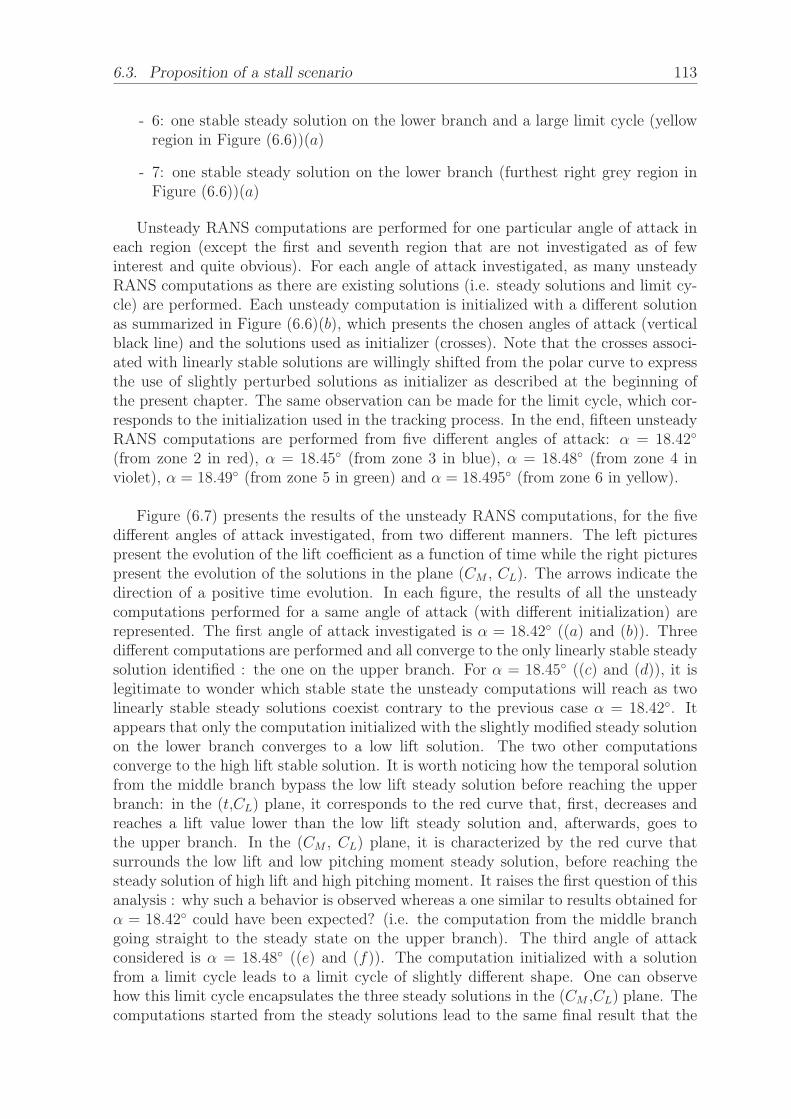
6.3. Proposition of a stall scenario 113
- 6: one stable steady solution on the lower branch and a large limit cycle (yellowregion in Figure (6.6))(a)
- 7: one stable steady solution on the lower branch (furthest right grey region inFigure (6.6))(a)
Unsteady RANS computations are performed for one particular angle of attack ineach region (except the first and seventh region that are not investigated as of fewinterest and quite obvious). For each angle of attack investigated, as many unsteadyRANS computations as there are existing solutions (i.e. steady solutions and limit cy-cle) are performed. Each unsteady computation is initialized with a different solutionas summarized in Figure (6.6)(b), which presents the chosen angles of attack (verticalblack line) and the solutions used as initializer (crosses). Note that the crosses associ-ated with linearly stable solutions are willingly shifted from the polar curve to expressthe use of slightly perturbed solutions as initializer as described at the beginning ofthe present chapter. The same observation can be made for the limit cycle, which cor-responds to the initialization used in the tracking process. In the end, fifteen unsteadyRANS computations are performed from five different angles of attack: α = 18.42◦
(from zone 2 in red), α = 18.45◦ (from zone 3 in blue), α = 18.48◦ (from zone 4 inviolet), α = 18.49◦ (from zone 5 in green) and α = 18.495◦ (from zone 6 in yellow).
Figure (6.7) presents the results of the unsteady RANS computations, for the fivedifferent angles of attack investigated, from two different manners. The left picturespresent the evolution of the lift coefficient as a function of time while the right picturespresent the evolution of the solutions in the plane (CM , CL). The arrows indicate thedirection of a positive time evolution. In each figure, the results of all the unsteadycomputations performed for a same angle of attack (with different initialization) arerepresented. The first angle of attack investigated is α = 18.42◦ ((a) and (b)). Threedifferent computations are performed and all converge to the only linearly stable steadysolution identified : the one on the upper branch. For α = 18.45◦ ((c) and (d)), it islegitimate to wonder which stable state the unsteady computations will reach as twolinearly stable steady solutions coexist contrary to the previous case α = 18.42◦. Itappears that only the computation initialized with the slightly modified steady solutionon the lower branch converges to a low lift solution. The two other computationsconverge to the high lift stable solution. It is worth noticing how the temporal solutionfrom the middle branch bypass the low lift steady solution before reaching the upperbranch: in the (t,CL) plane, it corresponds to the red curve that, first, decreases andreaches a lift value lower than the low lift steady solution and, afterwards, goes tothe upper branch. In the (CM , CL) plane, it is characterized by the red curve thatsurrounds the low lift and low pitching moment steady solution, before reaching thesteady solution of high lift and high pitching moment. It raises the first question of thisanalysis : why such a behavior is observed whereas a one similar to results obtained forα = 18.42◦ could have been expected? (i.e. the computation from the middle branchgoing straight to the steady state on the upper branch). The third angle of attackconsidered is α = 18.48◦ ((e) and (f)). The computation initialized with a solutionfrom a limit cycle leads to a limit cycle of slightly different shape. One can observehow this limit cycle encapsulates the three steady solutions in the (CM ,CL) plane. Thecomputations started from the steady solutions lead to the same final result that the

114 Chapter 6. Unsteady RANS simulations of the nonlinear dynamics
ω
σ
L
ω
σ
U
ω
σ
L
ω
σ
M
ω
σ
U
ω
σ
L
ω
σ
M
ω
σ
U
ω
σ
L
ω
σ
M
ω
σ
U
ω
σ
L
ω
σ
M
ω
σ
U
ω
σ
L
ω
σ
M
α = 18.42° :
α = 18.45° :
α = 18.48° :
α = 18.49° :
α = 18.495° : (j)
(h)
(f )
(d)
(b)
(i)
(g)
(e)
(c)
(a)
Figure 6.7: Temporal solutions represented in two different planes(t,CL) (left pictures) and (CM ,CL) (right pictures, also often called phaseportrait) for different initial conditions and angles of attack. (a) and (b):α = 18.42◦. (c) and (d): α = 18.45◦. (e) and (f): α = 18.48◦. (g) and(h): α = 18.49◦. (i) and (j): α = 18.495◦. For each angle of attack,the color of the curve refers to the color of the cross in Figure (6.6)(b),marking the solution used to initialize the unsteady computation indi-cated. The linear behavior of the steady solutions is recalled next to the
temporal solutions, as well as the angles of attack.

6.3. Proposition of a stall scenario 115
computation for α = 18.45◦ although the temporal solution from the middle branch(red curve) does not bypass the low lift low pitching moment solution, but goes straightto the high lift steady solution similarly to the case α = 18.42◦. The case α = 18.49◦
((f) and (g)) presents three computations: two from linearly unstable steady solutions(upper and middle branch), which reach the large limit cycle by oscillating around thethree steady solution for several periods and one from the slightly perturbed linearlystable steady solution on the lower branch, which returns to its stable steady state.Finally, the last angle of attack investigated is α = 18.495◦ ((i) and (j)) for which twotime-stepping computations are performed: one from a limit cycle and one from a lowlift solution. They respectively converge to a limit cycle and to a linearly stable steadysolution on the lower branch.
A few observations can be made from all these unsteady computations. First, theresults are qualitatively in perfect agreement with the linear stability analysis (one canrefer to appendix D for more details on the comparison between linear stability analysisand Unsteady RANS computations):
- The steady solutions for which a stable unsteady mode was found, are attractorsaround which the temporal solutions oscillate before converging towards it.
- The steady solutions for which an unstable unsteady mode was found, are re-pellers around which the oscillations of the temporal solution grow in time1.
- The steady solutions for which an unstable steady mode was found (mostly onthe middle branch) are repellers for which the temporal solutions directly divergefrom this solution without oscillating around it
Second, one can observe several noticeable features:
- Among all the time-stepping computations performed, the only ones that reach asteady low lift state are the ones initialized with a low lift steady solution. Neitherthe computations initialized with steady solutions from the upper and middlebranches nor the ones initialized with solutions from the limit cycle reach a lowlift steady state. In other words, all the time-stepping computations initializedwith linearly unstable steady solutions converge either to a high lift solution orto a large amplitude limit cycle.
- The results of the time-stepping computations initialized with steady solutionsfrom the middle branch are also quite interesting. These steady solutions arelinearly unstable and temporal solutions diverge from them towards a stablestate. It seems that as long as a linearly stable steady solution exists on theupper branch, the computations converge to this state (α = 18.42◦, α = 18.45◦
and α = 18.48◦) while, when the steady solutions on the upper branch becomeunstable, the time computations initialized from the middle branch reaches thestable limit cycle. Also, it is legitimate to wonder why the computations started
1It is not obvious for the computation initialized with the high lift unstable steady solution forα = 18.49◦ ((g) and (h)). However, two explanations can be proposed. First, the angular frequency ofthe stall mode associated with this steady solution is very low and, consequently, the oscillations aretoo slow to develop. Second, there is not a perfect match between the Unsteady RANS computationsand the linear stability analysis and the initialization would actually correspond to a steady solutionin the region labelled 3 in Figure 5.14 of chapter 5.

116 Chapter 6. Unsteady RANS simulations of the nonlinear dynamics
from the middle branch sometimes reach the steady state after surrounding thesolution on the lower branch (for example α = 18.45◦) and sometimes not (forexample α = 18.42◦ and α = 18.48◦)
6.4 ConclusionAlthough several differences between the time stepping methods in elsA and the con-tinuation methods were highlighted in chapter 4, the method detailed in appendix Cwas proven to successfully reconcile the results from the two approaches. Indeed, inthe present chapter, a very good agreement was shown between the linear behavior ofsteady solutions and the growth in time of the instabilities identified (also illustrated inappendix D). The two unstable modes identified appeared to develop into limit cyclesfor several values of angles of attack. In particular, the large limit cycle is identifiedfor several angles of attack at which very different steady states exist. A detailed in-vestigation is carried out in the stall area. Although the perfect agreement betweenthe linear stability analysis and unsteady RANS computations is again highlighted,this investigation seems to raise more questions than answers: why does the limit cyclesuddenly vanish for particular angles of attack? Why is there no consistency in theway the time-stepping computations starting from the middle branch reaches a stablestate? Why is it impossible to reach the limit cycle from steady solutions apart fromangles of attack at which an unstable steady solution exist on the upper branch? Whyis it impossible to reach a low lift steady state from any unstable steady state? Apossible answer to several of those questions could be the existence of unstable limitcycles, which cannot be detected with the approach considered in this chapter. Theobjective of the next chapter is to investigate this possibility and try to obtain a morecomplete bifurcation scenario.

117
Chapter 7
A static stall model based on thelinear analysis of RANS solutions
Contents7.1 Calibration of the one-equation static stall model . . . . . 118
7.1.1 Equation considered . . . . . . . . . . . . . . . . . . . . . . . 118
7.1.2 Calibration of the steady states . . . . . . . . . . . . . . . . . 119
7.1.3 Calibration of the linear behavior . . . . . . . . . . . . . . . . 119
7.1.4 Comparison of the position of the particular points of thesystem . . . . . . . . . . . . . . . . . . . . . . . . . . . . . . . 125
7.2 Nonlinear behavior of the static stall model . . . . . . . . 125
7.3 Comparison of the bifurcation scenario with the RANSapproach . . . . . . . . . . . . . . . . . . . . . . . . . . . . . . 128
7.3.1 Comparison of the range of existence of the limit cycles . . . 128
7.3.2 Comparison of the time evolution of the lift coefficient . . . . 128
7.3.3 Phase diagrams comparison . . . . . . . . . . . . . . . . . . . 132
7.3.4 Conclusion on the calibrated model . . . . . . . . . . . . . . . 136
7.4 Discussion of other possible scenarios . . . . . . . . . . . . 137
7.4.1 Approach and objectives . . . . . . . . . . . . . . . . . . . . . 137
7.4.2 Study of the nonlinear behavior in the case with hysteresis . . 138
7.4.3 Study of the nonlinear behavior in the case without hysteresis 144
7.5 Conclusion . . . . . . . . . . . . . . . . . . . . . . . . . . . . . 147
The linear stability analysis of the steady solutions revealed a complex scenario closeto stall (chapter 5). This scenario was confirmed by studying the nonlinear behavior ofthe flow with unsteady RANS computations, which also revealed a low frequency limitcycle of large amplitude. However, several points, detailed at the end of chapter 6,remain unclear. For instance, the appearance and disappearance of the limit cycle orthe impossibility to reach a low lift steady state from an unstable steady solution aretwo phenomena that cannot be explained with the available data. One of the possible

118 Chapter 7. A static stall model based on the linear analysis of RANS solutions
reason could be the existence of unstable limit cycles. Indeed, one of the limitation oftracking limit cycle with time steppers is the impossibility to identify unstable limitcycles. Specific tools exist in bifurcation theory to track these unstable limit cycles.However, their development in the RANS framework is not trivial and would be timeconsuming. Instead an alternative approach is considered: a one-equation nonlinearmodel, named static stall model is created. This model reproducing the linear behav-ior observed with the stability analysis is created and calibrated based on the steadyRANS solutions and their linear behavior. Then, by studying the nonlinear behavior ofthis model, it is expected to gain an understanding of the nonlinear mechanisms thatcould not be identified with unsteady RANS computations. The philosophy leading tothe considered form of the one-equation model is detailed in appendix E. Note that, thefinal form of the model is similar to a particular case of the more general Pernarowski’smodel [126] used in biophysics to study pancreatic beta cells. More details can be foundin the works of De Vries [35] and Fallah [52] in which curves very similar to the onesintroduced in this chapter can be encountered. In the end, the development of such amodel should allow us to have a better understanding of the nonlinear mechanisms ata reduced computational cost.
The first part of the chapter is dedicated to the calibration of the static stall model.Then, the nonlinear behavior of the calibrated model is studied and a bifurcationscenario is proposed. Finally, other possible scenarios are discussed.
7.1 Calibration of the one-equation static stall model
7.1.1 Equation considered
The equation of the model to be calibrated is presented in equation (7.1). The generalform of the equation remains the same as that introduced in equation (E.16) but theparameters B and C becomes higher order polynomials.
d2CL
dt2+ p1(CL) · dCL
dt+ c · (Δα + p2(CL)) = 0 (7.1)
where :
- p1(CL) =N1∑i=0
bi · C iL, with N1 the order of the polynomial p1(CL)
- p2(CL) =N2∑i=1
ai · C iL, with N2 the order of the polynomial p2(CL)
- Δα = α− αs, with αs an arbitrary defined stall angle
- CL = cl − cls , with cls the lift value associated to αS
Considering the decomposition CL = CL0 + C ′L, we obtain the equations at order
zero (ε0) and one (ε1).

7.1. Calibration of the one-equation static stall model 119
ε0 : Δα + p2(CL) = 0 (7.2)
ε1 :d2C ′
L
dt2+ p1(CL0) ·
dC ′L
dt+ c · ( dp2
dCL
(CL0)) · C ′L = 0 (7.3)
By similarity with the case of the damped harmonic oscillator presented in subsec-tion E.2.2, we define:
B = p1(CL0) (7.4)
C = c · dp2dCL
(CL0) (7.5)
Δ = B2 − 4 · C (7.6)
7.1.2 Calibration of the steady states
The first step is to arbitrary define a stall point (αs, cls), then we choose N points(αi,CL0i
) to fit and we solve the system (7.7) to find the N coefficients of the polynomialp2(x). ⎡
⎢⎣CL01
C2L01
. . . CNL01...
......
CL0NC2
L0N. . . CN
L0N
⎤⎥⎦ ·
⎡⎢⎣
a1...aN
⎤⎥⎦ =
⎡⎢⎣
−Δα1...
−ΔαN
⎤⎥⎦ (7.7)
A good fit is obtained with a 4th order polynomial and consequently no higher or-ders are investigated. The result of the calibration is presented in Figure (7.1).
7.1.3 Calibration of the linear behavior
7.1.3.1 Link between linear stability of RANS solutions and model param-eters
In the spirit of what was done for the simplest version of the one-equation model (seeappendix E), the parameters B and Δ are used to calibrate the linear behavior of themodel. As a reminder, B drives the position of the Hopf bifurcations (labelled H inchapter 5) while Δ drives the position of the steady solution with two identical eigen-values (labelled D in chapter 5). However, the result of the linear stability analysis ofthe steady RANS solutions did not provide values for B and Δ but a pair of eigenvalueλ1/2 for each angle of attack, characterized by their angular frequencies ω1/2 and theirgrowth rates σ1/2. First a link is established between the eigenvalues and the modelparameters B and Δ.

120 Chapter 7. A static stall model based on the linear analysis of RANS solutions
18.38 18.42 18.46 18.50
α(°)
1.20
1.25
1.30
1.35
1.40
1.45
1.50
1.55
CL
Figure 7.1: Calibration of the steady states. The black crosses markthe steady solutions from the RANS computations. The four red crossesare the steady solutions used for the fitting. The arbitrary stall angleand its associated lift coefficient is circled in red. The result of the fitting
operation is plotted in full black line.
- When the modes are steady, their angular frequencies are null (ω1/2 = 0). Thisleads to:
λ1/2 = σ1/2 =−B ±√
Δ
2(7.8)
- When the modes are unsteady, one is the complex conjugate of the other andtherefore they have the same growth rates (σ1 = σ2) and opposite angular fre-quencies (ω1 = −ω2). This leads to:
λ1/2 = σ1/2 + i · ω1/2 =−B ± i · √−Δ
2(7.9)
From equations (7.8) and (7.9), we can deduce the following link between the pa-rameters B and Δ and the components of the eigenvalues λ1/2:

7.1. Calibration of the one-equation static stall model 121
⎧⎪⎪⎪⎪⎪⎪⎪⎪⎪⎪⎪⎨⎪⎪⎪⎪⎪⎪⎪⎪⎪⎪⎪⎩
If ω1/2 = 0 :
B = −(σ1 + σ2)
Δ = (σ1 − σ2)2
If ω1/2 = 0 :
B = −(σ1 + σ2)
Δ = −(ω1 − ω2)2
(7.10)
with equations (7.10) it is now possible to determine a value of B and Δ for each angleof attack. Let us designate by Bcomp and Δcomp the values of B and Δ deduced fromthe results presented in chapter 5. The objective is now to find the best coefficients biand c, which appears in the parameters B and Δ in order to minimize the gap betweenthe experimental values Bcomp, Δcomp and the model values B, Δ. The mean leastsquare error is defined for each parameter :
BLMS =M∑i=1
[p1(CiL0)− Bcomp(λ
i1/2)]
2 (7.11)
ΔLMS =M∑i=1
[p1(CiL0)2 − 4 · c · dp2
dCL
(C iL0)−Δcomp(λ
i1/2)]
2 (7.12)
where M is the number of data from the computations considered for the calibration.
7.1.3.2 Non-dominated Sorting Genetic Algorithm II (NSGA-II)
The goal is now to minimize two objective functions at the same time for several pa-rameters (depending on the order N of the polynomial p1(x) considered). The maindifficulty in solving these kinds of problems is that there is no single solution thatminimizes both objective functions. Instead, several admissible solutions are founddepending on how one objective function is weighted compared to the other. Indeed,most of the time, a solution which minimizes an objective function will give poor resultson another objective function: the objective functions are defined as conflicting [50].In such a case, several Pareto optimal solutions exist. They correspond to the solutionsfor which the value of an objective function cannot be improved without degrading thevalues of the others.
A first approach to solve this multi-objectives problem could be to build a singleobjective function made of these two objective functions. This is the spirit of theobjective weighting approach, distance functions or min-max formulation. However,all these methods offer a single optimal solution to the problem heavily dependent onthe formulation used to build the scalar objective function. Moreover, it is difficult toprioritize the multiple objective functions a priori, during the building of the singleobjective function. One can find a summary of all these approach in the paper ofSrinivas and Deb [153]. An alternative to such methods is to try to obtain several

122 Chapter 7. A static stall model based on the linear analysis of RANS solutions
Pareto solutions in a single computation in order to be able to choose the solutionthe most adapted to the situation. This ensemble of solutions is called a Pareto front.Genetic Algorithms allow us to compute the solutions of this front. The particular caseof the Non-dominated Sorted Genetic Algorithm II (NSGA-II) [37] used in our case ispresented in more detail in appendix F.
7.1.3.3 Results of the calibration
The NSGA-II algorithm is used to calibrate the coefficients of the polynomial p1(x)and c. A third order polynomial is chosen for p1(x). The first reason for this choice isto have the same number of parameters and, thus, a similar precision on the calibra-tion of steady states and their linear stability. Also, it appears that higher order doesnot significantly improve the results. The Pareto front obtained (see appendix F formore details) is presented in Figure (7.2). Three particular solutions are highlightedto be presented in more detail: the blue point minimizes the error BLMS, the red pointminimizes the error ΔLMS and the green point is a compromise between the two.
0.000 0.001 0.002 0.003 0.004 0.005 0.006 0.007 0.008
Quadratic error on B: BLMS
0.000000
0.000002
0.000004
0.000006
0.000008
0.000010
0.000012
Quadra
tic e
rror
on Δ
: ΔLMS
Figure 7.2: Pareto front obtained for the calibration of the linear be-havior. Three solutions are highlighted to be presented in more detail.
Figure (7.3) compares the evolution of four variables as a function of the angle ofattack between different calibration of the model and the results of the RANS compu-tations: B (picture a), Δ (picture b), σ (picture c) and ω (picture d). Figure (7.3)(a)confirms that the blue solution, which minimizes the least mean square error on B,is the best fit for B, while the red solution, which maximizes the least mean squareerror on B, is the worst fit. Figure (7.3)(b) shows the exact opposite for the parameterΔ. For both variables, the green solution, stands in between these two extrema, rep-resenting a compromise between the two solutions. Figures (7.3)(c) and (d) show thata better fit on B (blue solution) corresponds to a better fit on the growth rate, while

7.1. Calibration of the one-equation static stall model 123
(a) (b)
(c) (d)
Figure 7.3: Evolution of four variables as a function of the angle ofattack. (a): B. (b): Δ. (c): σ. (d): ω. Three different calibrationsobtained with the NSGA-II algorithm are presented. The colors of thecurves correspond to the solutions highlighted in Figure (7.2). The evo-lutions of the variables from the model are compared with the associatedvariables obtained from the stability analysis of steady RANS solutions
(black dots).
a better fit on Δ ensures a better fit on the angular frequency.
Figure (7.4) presents the superimposed spectra obtained for the three calibrations.The blue solution, which minimizes the error on B and on the growth rate σ seemsto correctly reproduce the positions where the eigenmodes switch from steady to un-steady but fails to reproduce the parabolas made by the eigenmodes. On the otherhand, the red solution perfectly reproduces the parabolas of the spectrum but fails to

124 Chapter 7. A static stall model based on the linear analysis of RANS solutions
catch the position at which the mode switches from unsteady to steady on the upperbranch (furthest left parabola). The green solution offers very decent results on the twofeatures. Note that the eigenvalues on the upper branch (furthest left parabola) aremore sensitive to the different solutions than the lower branch (furthest right parabola).
(a) (b) (c)
Figure 7.4: Comparison of the superimposed spectra obtained for dif-ferent calibration of the model (color dots) with the superimposed spec-tra obtained from the stability analysis of steady RANS solutions pre-sented in Figure (5.13) in section 5 (black dots). The colors of the spectra
correspond to the solutions highlighted in Figure (7.2).
Based on these observations, the solution represented in green in the Pareto frontplotted in Figure (7.2) is chosen. The corresponding coefficients, used for the study ofthe nonlinear behavior of the model, are presented in Table 7.1.
Coeff Value Coeff Value Coeff Value
αs 18.4381 a1 −1.0049 b0 −1.8359× 10⁻²
CLs 1.3651 a2 −1.2304× 10⁻¹ b1 6.9644× 10⁻²
c 2.8708× 10⁻⁴ a3 51.7158 b2 1.4837a4 19.7393 b3 1.2870
Table 7.1: Values of the different coefficients corresponding to thechosen solution.

7.2. Nonlinear behavior of the static stall model 125
7.1.4 Comparison of the position of the particular points of thesystem
Table 7.2 presents the positions of some specific points obtained from the one-equationstatic stall model and from the RANS computations (introduced in Table 5.3 of chap-ter 5). For each branch, the three points considered are the Hopf bifurcations (notedH), the solutions with two identical eigenvalues (noted D) and the saddle-node bifur-cations (noted SN). In order to compare the results a relative error on the position isintroduced. The following characteristic scales are used:
- Saddle-node bifurcations: the range of the hysteresis (i.e. Δα between the twosaddle-node bifurcations)
- Hopf bifurcations: the range in which unstable modes exist on the consideredbranch (i.e. the gap between the Hopf bifurcation and the closest saddle-nodebifurcation)
- Two identical eigenvalues point: the range in which steady modes exist on theconsidered branch (i.e. the gap between the two identical eigenvalues point andthe closest saddle-node bifurcation)
First, one can observe that the positions of the saddle-node bifurcations are wellreproduced by the model with a very low relative error on the estimation of their po-sitions. Indeed, the calibration of the steady states (from which the position of thesaddle-nodes is determined) is more accurate than the one of the linear behavior. Sec-ond, the points H and D are better estimated on the lower branch than on the upperbranch. This result was expected based on the observations made during the anal-ysis of the spectra from different calibration in the Pareto front presented in Figure(7.2). On the upper branch, the points are closer to the saddle-node bifurcations forthe model than for the RANS computations. The consequence is that the point withtwo identical eigenvalues is almost superposed with the saddle-node bifurcation. Onthe lower branch, the position of the Hopf bifurcation is pretty well estimated whilethe position of the solution with two identical eigenvalues exhibits a non negligiblerelative error. Generally speaking, the range of existence of the two unstable steadyeigenvalues is very tiny (as shown in Figure (5.13) in chapter 5), which explains why asmall difference of positioning leads to a large relative error.
7.2 Nonlinear behavior of the static stall modelA set of parameters offering the best fit between the linear behavior of the model andthe linear behavior of the steady RANS solutions is found. The nonlinear behavior ofthe model is investigated with this set of parameters to gain an understanding of thenonlinear behavior of the RANS computations. Matcont [39], a Matlab Plug-in madefor numerical continuation and bifurcation study of parametrized dynamical systems,is used to perform this study. It offers a fast and easy way to obtain solutions intime and compute steady states and limit cycles with continuation methods. Thenumerical aspect of Matcont is not described but all the techniques used in this study

126 Chapter 7. A static stall model based on the linear analysis of RANS solutions
RANS Model L Error (%)
Upper branchH 18.4867 18.4912 0.00533 84.43D 18.4919 18.4920267 0.00013 97.46SN 18.49203 18.4920274 0.1078 O(10−3)
Lower branchH 18.4527 18.4529 0.06847 0.29D 18.3846 18.3847 0.00037 27.03SN 18.38423 18.38417 0.1078 O(10−2)
Table 7.2: Comparison of RANS computations and the static stallmodel for three particular points: Hopf bifurcation H, two identicaleigenvalues D and saddle-node bifurcation SN. L designates the charac-
teristic scale used to compute the relative error in %.
(definition of the stall model in Matcont, steady solutions computation, time-steppingcomputations, limit cycle identification, limit cycle tracking,...) are detailed in tutorials[103] and [104]. The results of the analysis are depicted in Figure (7.5), which presents:(a) the polar curve zoomed in close to stall angle and the existing limit cycles (providinga bifurcation diagram close to stall) and (b) schematic phase diagrams for nine valuesof α (representation freely inspired from the ones found in the book of Kuznetsov aboutbifurcation theory [89]).
Starting from the lowest value of α on the upper branch, one can observe, in phasediagram 1, a single stable steady solution to which all trajectories converge. Closeto the steady point, the trajectories form a focus, indicating that a pair of complexconjugate eigenvalues is stable. By increasing the angle of attack, three steady solutionscoexist: the stable focus on the upper branch and two unstable steady solutions. Asseen in the phase diagram 2, the steady solution on the middle branch is a saddlepoint, indicating the existence of two steady eigenvalues, one stable and one unstable.On the other hand, the steady solution on the lower branch is a focus, indicatingthat a pair of complex eigenvalues is unstable. Obviously, all the trajectories convergetowards the only stable solution on the upper branch. By further increasing α, a Hopfbifurcation occurs on the lower branch of steady solutions as the unstable unsteady pairof eigenvalues become stable on this branch. Moreover, an unstable branch of limitcycles emerges for higher angles of attack from this Hopf bifurcation, indicating thatit is subcritical. Phase diagram 3 illustrates the existence of the unstable limit cycle.It surrounds the stable steady solution on the lower branch, dividing the solution fieldinto two parts: inside the limit cycle, the trajectories converge to the lower branch and,outside, to the upper branch. For higher angles of attack, a homoclinic bifurcation isencountered as illustrated in phase diagram 4. It is characterized by a trajectory whichstarts from the middle branch and ends to the same solution, circling the two othersteady solutions. Further increasing the angle of attack, it appears that this homoclinicorbit actually results from the collision of a large limit cycle (visible in phase diagram5) with the saddle point on the middle branch of steady solutions. Note that thecollision occurs via a shrink of the limit cycle in the direction CL. This explains why itis not visible in the bifurcation diagram shown in (a), which displays CL as a functionof α. In the phase diagram 5, two limit cycles coexist, the large one being stable whilethe small one surrounding the lower steady state is still unstable. Between these two

7.2. Nonlinear behavior of the static stall model 127
18.4 18.42 18.44 18.46 18.48 18.5
1.1
1.15
1.2
1.25
1.3
1.35
1.4
1.45
1.5
1.55
CL
α (°)
1
2
3
4 5
9
8
7
6
1 2 3
4 5 6
7 8 9
(a) (b)
Figure 7.5: (a) Bifurcation diagram from the calibrated stall model(parameters presented in table parameters). The color code of the steadystates is similar to the one used in Figure (5.13) (i.e. Blue: two unsteadyeigenvalues. Red: two steady unstable eigenvalues. Green: two steadyeigenvalues, one stable and one unstable). The limit cycles are repre-sented with black lines corresponding to the evolution of their extremevalues. Steady solutions and limit cycles are represented such that: fulllines indicate stable states and dashed lines indicate unstable states. (b)Schematic phase diagrams in the plane (CL, CL) for different values ofα referenced in the bifurcation diagram (a). The arrows in the phase
diagram indicate a positive evolution of time.
limit cycles, the trajectories can either converge to the large limit cycle or to the uppersteady solution. When α is further increased, a second homoclinic bifurcation occurs(phase diagram 6 and 7) via the collision of an unstable upper limit cycle with themiddle sadde point. For this second homoclinic bifurcation, the unstable limit cycleemerges from the subcritical Hopf bifurcation on the upper branch of steady solutions.Examining phase diagrams 6 and 7, one can observe a shrink of the limit cycle inthe CL (vertical) direction which makes it clearly visible in the bifurcation diagram(a). Further increasing the angle of attack, the unstable upper limit cycle vanishes at aHopf bifurcation on the upper branch. Once going through the saddle-node bifurcationon the upper branch, there are only two limit cycles remaining in phase diagram 8,coexisting with the stable lower steady solution. Finally, the size of the unstable lowerlimit-cycle grows until it collides with the large stable limit cycle in phase diagram 9.This is a saddle-node bifurcation of periodic orbits that leads to their disappearance.Thus, only the lower steady solution exists for larger values of α.

128 Chapter 7. A static stall model based on the linear analysis of RANS solutions
7.3 Comparison of the bifurcation scenario with theRANS approach
This section is dedicated to the comparison between the bifurcation scenario suggestedby the static stall model and the results of the unsteady RANS computations. Thefeatures of the stable large limit cycle are discussed, the time evolution of the liftcoefficients are compared and the phase diagrams presented in Figure (7.5)(b) areconfronted to the ones presented in Figure (6.7) of chapter 6. Throughout the wholeanalysis process, answers to the questions raised by the unsteady RANS computationsare proposed. Finally, the limitations of the model such as calibrated are discussed.
7.3.1 Comparison of the range of existence of the limit cycles
Figure (7.6) shows the complete bifurcation scenario obtained with the model : thesteady states and the limit cycles. The limit cycles obtained with the unsteady RANScomputations are superimposed to this diagram for comparison matters. One cannote that the stable limit cycle observed with the unsteady RANS computation isqualitatively similar to the one observed with the static stall model. Indeed, in bothcases, the smallest value of α for which it exists is associated with stable steady solutionson the upper and lower branches and unstable on the middle branch (states 3 and 4 ofFigure (6.6 of chapter 6) and the highest value of α for which it exists is associated to theexistence of a unique steady solution on the lower branch (states 6 and 7 of Figure (6.6of chapter 6). However, the one caught with the unsteady RANS computations is largerthan the one predicted by the model (ΔCL ≈ 0.5 and ΔCL ≈ 0.4 respectively), wider(Δα ≈ 0.035◦ and Δα ≈ 0.02◦ respectively) and slightly shifted to the left (smallestangle of attack at which it exists: α ≈ 18.46◦ and α ≈ 18.482 respectively). In theend, the nonlinear behavior of the model, although not being in perfect agreementwith unsteady RANS computations, qualitatively well predicts the main features ofthe stable limit cycle. This indicates that it is meaningful to investigate and study inmore detail the unstable limit cycles revealed by the static stall model.
7.3.2 Comparison of the time evolution of the lift coefficient
In chapter 6, five different areas (presented in Figure (6.6)) were considered and, foreach one, unsteady computations were performed for a particular angle of attack. Foreach angle of attack considered, computations were initialized with different solutions(i.e. each steady solution existing for this particular value of α and, if existing, froman extremum point of a limit cycle as presented in Figure (6.7)). As a reminder, thefive zones considered are listed below :
- 2: one stable steady solution on the upper branch and two unstable steady solu-tions on the middle and lower branches
- 3: two stable steady solutions on the upper and lower branches and an unstablesteady solution on the middle branch
- 4: two stable steady solutions on the upper and lower branches and an unstablesteady solution on the middle branch and a large limit cycle

7.3. Comparison of the bifurcation scenario with the RANS approach 129
18.4 18.42 18.44 18.46 18.48 18.51
1.05
1.1
1.15
1.2
1.25
1.3
1.35
1.4
1.45
1.5
1.55
1.6
CL
α (°)
Figure 7.6: Comparison of the nonlinear behavior of the model and theresults of unsteady RANS computations. The full red lines correspondto the extreme values of the limit cycles identified with unsteady RANS
computations.
- 5: one stable steady solution on the lower branch and two unstable steady solu-tions on the middle and upper branches and a large limit cycle
- 6: one stable steady solution on the lower branch and a large limit cycle
A similar division can be considered in the bifurcation diagram of the static stallmodel (although the range of each zone will be slightly shifted due to the calibration)and time-stepping computations of the static stall model are performed for: α = 18.42◦
(2), α = 18.46◦ (3), α = 18.485◦ (4), α = 18.4915◦ (5) and α = 18.495◦ (6). The an-gles of attack considered are different from the ones chosen for the unsteady RANScomputations but there is still one in each area to compare each other. The resultsobtained, presented in Figure (7.7), are to be compared to the ones obtained with un-steady RANS computations and presented in Figure (6.7) in chapter 6. For each case,the time evolution of the lift coefficient is qualitatively very similar for the static stallmodel and for the unsteady RANS computations. The only difference comes from theamplitude of the oscillations as already illustrated in Figure (7.6) and the exact anglesof attack considered.
The main advantages of this static stall model are its very low computational cost,which, for instance, allows us to perform a detailed influence of the initial condition,and its capacity to detect unstable limit cycles. Several phenomena, very difficult toidentify with unsteady RANS computations, can be easily identified with time-steppingcomputations of the static stall model. In order to describe them, zone 4 is studied inmore detail. By applying the method used to define the zones, it appears that this zone

130 Chapter 7. A static stall model based on the linear analysis of RANS solutions
18.4 18.42 18.44 18.46 18.48 18.5
1.1
1.15
1.2
1.25
1.3
1.35
1.4
1.45
1.5
1.55
CL
α (°)0 500 1000 1500 2000 2500
1.15
1.2
1.25
1.3
1.35
1.4
1.45
1.5
1.55
t
CL
0 400 800 1200 1600 20001.05
1.1
1.15
1.2
1.25
1.3
1.35
1.4
1.45
1.5
1.55
t
CL
0 1000 2000 3000 40001.05
1.1
1.15
1.2
1.25
1.3
1.35
1.4
1.45
1.5
1.55
t
CL
0 1000 2000 3000 40001.05
1.1
1.15
1.2
1.25
1.3
1.35
1.4
1.45
1.5
1.55
t
CL
(a)
(c)
(e)
(b)
(d)
(f )
0 1000 2000 3000 40001.05
1.1
1.15
1.2
1.25
1.3
1.35
1.4
1.45
1.5
1.55
t
CL
Figure 7.7: Time evolution of the lift coefficient obtained with thestatic stall model from different values of α. The crosses correspond tothe steady solutions used to initialize the unsteady computations. (a)Bifurcation diagram from Figure (7.5) and angles of attack considered.(b) α = 18.42◦. (c) α = 18.46◦. (d) α = 18.485◦. (e) α = 18.4915◦. (f)α = 18.495◦. The color code of the crosses in (a) matches the one of the
curves in (b), (c), (d), (e) and (f).

7.3. Comparison of the bifurcation scenario with the RANS approach 131
18.4 18.42 18.44 18.46 18.48 18.5
1.1
1.15
1.2
1.25
1.3
1.35
1.4
1.45
1.5
1.55
CL
α (°)18.48 18.4918.47 18.5
1.4
1.45
1.5
CL
α (°)
CL
0 1000 2000 3000 40001.05
1.1
1.15
1.2
1.25
1.3
1.35
1.4
1.45
1.5
1.55
t0 1000 2000 3000 4000
1.05
1.1
1.15
1.2
1.25
1.3
1.35
1.4
1.45
1.5
1.55
t
CL
(a)
(c)
(b)
(d)
Figure 7.8: Time evolution of the lift coefficient obtained with thestatic stall model from different values of α. The crosses correspond tothe steady solutions used to initialize the unsteady computations. (a)Bifurcation diagram from Figure (7.5) and angles of attack considered.(b) (a) Bifurcation diagram from Figure (7.5) zoomed in area 4 andangles of attack considered. (c) α = 18.485◦. (d) α = 18.4905◦. Thecolor code of the crosses in (a) and (b) matches that the curves in (c)
and (d).
can actually be split into two different zones because of the existence of the unstablelimit cycle emerging from the Hopf bifurcation on the upper branch. A first subregion4a can be defined from the lowest angle of attack for which the stable limit cycle existto the point where the unstable limit cycle from the upper branch ends (i.e. whenit collides with the middle branch of steady solutions in a homoclinic bifurcation).A second subregion 4b can be defined in all the range of existence of this unstablelimit cycle, from the homoclinic bifurcation to the Hopf bifurcation. The differencebetween those two subregions is illustrated in Figure (7.8), which presents results fortime-stepping computations at α = 18.485◦ (in area 4a, already presented in Figure(7.7)) and α = 18.4905 (in area 4b). The only difference between the two zones is en-countered for temporal computations starting from the middle branch, consequently,only this case is presented in Figure (7.8).

132 Chapter 7. A static stall model based on the linear analysis of RANS solutions
Figures (7.8)(a) and (b) present the position of the steady solutions considered forthe initializations of the two computations and Figure (7.8)(c) and (d) the evolution ofthe lift coefficient as a function of time for the associated computations (α = 18.485◦
and α = 18.4905 respectively). One can observe how the unstable limit cycle existingin zone 4b acts as a repeller. It prevents the temporal solution to reach the stablesteady state on the upper branch and forces it to converge to the stable limit cyclewhile, without the existence of this limit cycle (zone 4a), the solution converges to thestable steady solution on the upper branch (full red line). The deviation generatedby the unstable limit cycle is clearly between t ≈ 500 and t ≈ 700 in Figure (7.8)(d).Based on these results and assuming that the static stall model correctly predicts theexistence of unstable limit cycles, one can deduce that α = 18.48◦ is located in thearea 4a, before the appearance of the unstable limit cycle. Indeed, it would have beenimpossible to reach the upper branch from the middle branch if it was located in 4b,when this unstable limit cycle exists (see Figure (6.7) in chapter 6). The second infor-mation is deduced by slightly modifying the steady solution on the middle branch usedto initialize the computation (a variation of lift of ΔCL = 10−3 is considered). Theresults are presented in Figure (7.8)(c), which compares the time evolution previouslydescribed (full red line) to a computation initialized with a slightly modified steadysolution (dashed red line). A tiny modification of the initial condition leads to a majorchange of result as, instead of converging towards the stable steady state on the upperbranch, the large limit cycle is reached. To understand this behavior, we can refer tothe phase diagram number 5 presented in Figure (7.5). If the time-stepping computa-tion is initialized with a solution located in the area delimited by the two lines thatconverge to the steady solution on the middle branch, it will converge to the upperbranch, otherwise, it will converge to the limit cycle. Explained in a simpler manner:for CL = 0 a computation initialized with a solution slightly above the steady solutionon the middle branch will converge to the upper branch whereas a computation initial-ized slightly below will reach the stable large limit cycle. This sensitivity to the initialconditions is also probably at the origin of a phenomenon identified in Figure (6.7):unsteady RANS computations initialized from the middle branch sometimes convergedstraight to steady solution on the upper branch (α = 18.42◦ and α = 18.48◦) andsometimes went around the low lift solution before converging to the steady solutionon the upper branch (α = 18.45◦). These observations enlighten us on the fact that theunsteady RANS computations could have given very different results if started withslightly different flow topologies of angles of attack, especially in area 4.
7.3.3 Phase diagrams comparison
In Figure (6.7) of chapter 6, the results of the unsteady computations were plotted inthe plane (CM , CL), which is very similar to the phase diagrams describing the stallmodel in Figure (7.5). This subsection is dedicated to the comparison of the phasediagrams from the unsteady RANS computations with phase portraits from the staticstall model for the different zones identified.

7.3. Comparison of the bifurcation scenario with the RANS approach 133
(f )
(d)
(b)
(e)
(c)
(a)
α(° )18.4 18.45 18.5
1
1.2
1.4
1.6
CL
18.4 18.44 18.48
1.1
1.2
1.3
1.4
1.5
CL
α (°)
2
4
5
6
3
Figure 7.9: Comparison of phase diagrams (1/2). Polar curve andextreme values of limit cycle from unsteady RANS computations (a)and from the static stall model (b). Vertical lines in (a) mark the an-gles of attack considered and the crosses, the solutions used to initializethe unsteady RANS computations. The five cases considered for themodel are marked by arrows and referenced by the number of the areain (b). Results of the unsteady RANS computations presented in theplane (CM , CL) for (c) α = 18.42◦ and (e) α = 18.45◦. Correspond-ing schematic phase diagram in the plane (CL, CL) determined with thestatic stall model for (d) zone 2 and (f) zone 3. The colors used tomark the initial point in the polar curve and to draw the lines in the cor-responding phase diagrams all match. The grey lines in the schematicphase diagrams are the results observed with the model but not con-
firmed with unsteady RANS computations.

134 Chapter 7. A static stall model based on the linear analysis of RANS solutions
(f )
(d)
(b)
(e)
(c)
(a)
Figure 7.10: Comparison of phase diagrams (2/2). Results of theunsteady RANS computations presented in the plane (CM , CL) for (a)α = 18.48◦ (c) α = 18.49◦ and (e) α = 18.495◦. Correspondingschematic phase diagram in the plane (CL, CL) determined with thestatic stall model for (b) zone 4, (d) zone 5 and (f) zone 6. The colorsused to mark the initial point in the polar curve and to draw the linesin the corresponding phase diagrams all match. The grey lines in theschematic phase diagrams are the results observed with the model but
not confirmed with unsteady RANS computations.
The results of the comparison between the two approaches are depicted in Figures(7.9) and (7.10). Figure (7.9)(a) presents the incomplete bifurcation diagram obtainedin the RANS framework in which the angles of attack considered are indicated as well asthe initializer of the unsteady computations. Figure (7.9)(b) presents the correspond-ing zones in the bifurcation diagram from the static stall model. Figures (7.9)(c) and

7.3. Comparison of the bifurcation scenario with the RANS approach 135
(e) and (7.10)(a), (c) and (e) exhibit the results of the unsteady RANS computationsin the plane (CM , CL), already presented in Figure (6.7) of chapter 6. Figures (7.9)(d)and (f) and (7.10)(b), (d) and (f) exhibit schematic phase diagrams from the study ofthe static stall model. The colored lines correspond to the trajectories identified withunsteady RANS computations while grey lines correspond to information not detectedwith unsteady RANS computations. The first thing to notice is that, in the schematicrepresentation of the model, the three steady solutions (when existing) have the sameCL value (horizontal axis) and are aligned. This is not the case for the results fromunsteady RANS computations, which exhibits different values of pitching moment co-efficient CM for each steady solution. This difference is due to the fact that the staticstall model was calibrated based on lift coefficient evolution only and, consequently,only the CL variable has a non-null steady state. A possible improvement of the modelwould be to take the pitching moment into account in the calibration process. Sec-ond, note that all the trajectories identified with the unsteady RANS computationsare spotted with the study of the static stall model.
Moreover, the additional information provided by the static stall model, inaccessiblewith unsteady RANS computations (or at a very high computational cost), allows usto answer most of the questions raised at the end of chapter 6.
- Regarding the appearance and disappearance of the stable limit cycle, it is ac-tually a homoclinic bifurcation for the lowest values of α at which it exists anda saddle-node bifurcation of periodic orbits for the highest values of α at whichit exists. The criticaliity of the Hopf bifurcations is also determined: they aresubcritical. The unstable limit cycle emerging from the Hopf bifurcation on theupper branch disappears in a homoclinic bifurcation, while the unstable limitcycle emerging from the Hopf bifurcation on the lower branch is directly relatedto the stable limit cycle in the aforementioned saddle-node bifurcation of periodicorbits.
- The impossibility to reach a steady solution on the lower branch from any otherbranch is attributed to the presence of the unstable limit cycle surrounding thelower branch of steady solutions and clearly visible in Figures (7.9) (f) and(7.10)(b) and (d).
- The different trajectories identified for computations initialized from the middlebranch were attributed to the sensitivity of the initial condition in this region(section 7.3.2). It is clearly confirmed in Figures (7.9)(d) and (f) and (7.10)(b)and (d), where two trajectories depart from the steady solution on the middlebranch in opposite directions. Furthermore, it appears that the choice of initialcondition can affect not only the trajectory but also the stable state reached asillustrated in Figure (7.10)(b), which was not considered based on the results ofunsteady RANS computations.
- The unsteady RANS computations performed tended to prove that the stablelimit cycle could be reached from unstable steady solutions only in zone 5 (Figure(7.10)(c) and (d)). However, the static stall model demonstrates that it is alsopossible to reach this limit cycle from the middle branch in zones 4a (Figure(7.10)(a) and (b)) and 4b.

136 Chapter 7. A static stall model based on the linear analysis of RANS solutions
7.3.4 Conclusion on the calibrated model
Finally, the static stall model, which appears to be in excellent agreement with theunsteady RANS computations, provides a complete bifurcation diagram. Based on allthese information, it is possible to determine towards which stable state a time-steppingcomputation would converge based on its initialization. This is summarized in Figure(7.11) in which four distinct areas are identified :
- The yellow area, in which computations converge to the upper branch. This areacovers most of the hysteresis and is stopped by the appearance of the unstablelimit cycle from the lower branch and the large stable limit cycle. There is alsoa pocket inside the unstable limit cycle from the Hopf bifurcation on the upperbranch.
- The orange area, in which the computations converge either to the upper branchor the stable limit cycle. This area is located inside the unstable limit cycle fromthe Hopf bifurcation on the lower branch and expands when the large limit cyclevanishes.
- The pink area, in which the computations converge either to the stable limitcycle or to the upper branch. This area is located inside the large limit cycle,before the appearance of the unstable limit cycle from the Hopf bifurcation onthe upper branch.
- The violet area, in which computations converge to the lower branch. This areais located outside the large limit cycle when it exists and between the large limitcycle and the unstable limit cycles when the unstable limit cycle from the Hopfbifurcation on the upper branch appears.
However, it was shown that although providing results qualitatively in good agree-ment with unsteady RANS computations, the static stall model suffers from somelimitations regarding a quantitative comparison. Two main reasons can be responsiblefor the differences noticed. The first one is attributed to the calibration process, whichinvolves a multi-objective minimisation that ends up being a compromise between twoobjective functions. The main drawback of this approach is to have to choose one solu-tion among the others on the Pareto front, which are all, according to the optimizationprocess, similarly "good" solutions. As a reminder, one objective function mostly drivesthe evolution of the angular frequency of the eigenvalues while the other mostly drivesthe evolution of the growth rate of the eigenvalues. Thus, the Hopf bifurcations requirea correct estimation of the change of sign of the growth rate to be well estimated whilethe solution with two identical eigenvalues requires a correct estimation of the momentthe angular frequency becomes null. Consequently, by definition of a compromise, itwill not be possible to exactly estimate the position of these two particular points onthe two branches at the same time. This error in the calibration of the linear states ofthe model probably leads to differences on the nonlinear behavior of the model. Onecan suppose that a better calibration or formulation of the linear states of the modelcould improve the modeling of the nonlinear behavior. The second reason is that, asexplained in chapter 4 and developed in appendix C, there is a difference between thesteady solutions obtained with continuation methods and the ones obtained with alocal time stepping approach. It was identified that the main difference between the

7.4. Discussion of other possible scenarios 137
To the upper branch
To the lower branch
To the upper branch
or the limit cycle
To the limit cycle
18.4 18.42 18.44 18.46 18.48 18.51
1.05
1.1
1.15
1.2
1.25
1.3
1.35
1.4
1.45
1.5
1.55
1.6
CL
α (°)
Figure 7.11: Presentation of the four basins of attraction that affectthe result of the unsteady computations based on the position of the
initial solution in the plane (CL, α) for CL = 0 .
two approaches is the presence of cutoffs in one case and not in the other. These cut-offs are also implemented and active in the unsteady RANS equations solver. It wasdemonstrated that a slight modification of one cutoff ensures a better match betweenthe steady solutions obtained with the two methods (see appendix C) and, supposedly,it ensures a good match between the linear behavior of those steady solutions andunsteady RANS computations. However, the correction proposed does not provideperfect results and a tiny error still remains. Due to the small range of angles of attackin which all these phenomena occur, this error can be non negligible. Ideally, one wouldhave wanted to modify the formulation of the Spalart–Allmaras turbulence model inelsA in order to remove the cutoffs. However, this would be highly time consuming andpossibly tricky to achieve, which explains why the compromise of the modification ofone cutoff was adopted. In the end, the two sources of differences between the modeland the RANS computations lead to one main question: how do those errors influencethe results of the nonlinear behavior? Indeed, it was argued that they only affect thevalues of the results but not the general behavior of the bifurcation scenario. However,it is legitimate to wonder to what extent this statement is true. The next section triesto provide an answer to this question.
7.4 Discussion of other possible scenarios
7.4.1 Approach and objectives
In order to evaluate to what extent an error in the calibration process could affect thebifurcation scenario, the simplest form of the static stall model is considered and the

138 Chapter 7. A static stall model based on the linear analysis of RANS solutions
influence of a reduced number of parameters on the nonlinear behavior is studied. Theequation considered, given in (E.16), is recalled in (7.13) and corresponds to the mostbasic form for which the main features of the linear behavior are reproduced:
d2cldt2
+ (2 · b+ c2l ) ·dcldt
+ c · (α + d · cl + c3l ) = 0 (7.13)
The objective is to identify the influence of the parameters of the model on the non-linear behavior. Three parameters drive the whole model: b, c and d. The parameterd is responsible for the appearance of hysteresis in the steady solutions. In appendixE, it is set to d = −1 to ensure the appearance of this particular "S" shaped curvecharacterizing the hysteretic area. The study of the influence of the parameters is per-formed in two steps: first, the influence of b and c is investigated with the parameterd set to d = −1 and, afterwards, the influence of the parameters b and c with d = 1 isperformed. Note that with such a shape, the point (0, 0) is the center of symmetry ofthe steady solutions and their associated linear behavior.
7.4.2 Study of the nonlinear behavior in the case with hystere-sis
The five scenarios are presented in Figures (7.12) to (7.16). For each figure, the branchesof steady-state and limit-cycle solutions are shown in (a) by displaying the lift coeffi-cient cl as a function of the angle of attack α. The colored curves represent the steadystate solutions while the black curves correspond to the extreme values of the limit-cycle solutions. In (b), several solutions are displayed in the phase space (dcl
dt, cl) for
particular values of α corresponding to the numbers indicated in (a). The values ofthe parameters b and c are tested in ranges defined in (E.27) to ensure that the linearbehavior of the one equation model is coherent with the linear behavior of the steadyRANS solutions. Five different behaviors are observed and presented in the following.For each scenario, the general behavior of the steady solutions and their linear stabil-ity is similar. The difference comes from the exact position of the Hopf bifurcation(labelled H in chapter 5), the point where the eigenvalues switch from complex to real(labelled D in chapter 5) and the growth of the limit cycles.
7.4.2.1 First scenario: b = −0.42 and c = 0.1
Reading the bifurcation diagram of Figure (7.12) from left to right, one can first ob-serve one steady stable solution. In the corresponding phase diagram, this stable steadysolution is a focus point to which all trajectories converge. Then, by increasing thevalue of α, three steady solutions coexist: one stable solution on the upper branchand two unstable solutions on the middle and lower branches shown with dots. Theassociated phase diagram (number 2) shows that all the trajectories converge to thestable solution no matter the initial point in the phase space. Further increasing theangle of attack, the steady unstable eigenvalue of the steady solution on the lowerbranch becomes an unsteady unstable eigenvalues. Instead of diverging straight fromthis point, the temporal solutions are now orbiting around it as they diverge, as shownin the phase diagram 3. However, all trajectories converge towards the upper branch.

7.4. Discussion of other possible scenarios 139
α
CL
(a) (b)
654
321
16
2
3
45
Figure 7.12: First stall scenario. (a) Schematic bifurcation diagramincluding steady solutions (in colored lines) and extreme values of limitcycles (black lines) in the plane (cl, α). (b) Schematic phase diagrams inthe plane (cl, cl) for different values of α referenced on the bifurcation
diagram.
Then, the Hopf bifurcation on the lower branch gives birth to an unstable limit cyclewhen the steady solution on the lower branch is stabilized (phase diagram 4). All thecomputations started inside the limit cycle will converge to the lower branch whereas allthe other ones will converge to the steady solution of the upper branch. When increas-ing the parameter α, the radius of the limit cycle grows until the limit cycle collideswith the steady solution of the lower branch, as shown in the phase diagram 5. Thiscollision is characteristic of a homoclinic bifurcation and leads to the disappearance ofthe limit cycle. The phase diagram number 6 exhibits two stable steady solutions onthe upper and lower branches and an unstable steady solution on the middle branch.Each stable solution can be reached depending on the point in the phase space chosenfor the initialisation. Finally, when further increasing the angle of attack, a similarscenario is observed, but in reversed order (from 6 to 1) and by replacing the role ofthe lower and upper branches. In this first reference scenario, the Hopf bifurcationslead to the appearance of unstable limit cycles, but no stable limit cycle is observed.
7.4.2.2 Second scenario: b = −0.42 and c = 0.5
The second stall scenario found with the one-equation stall model is described in Figure(7.13). Similarly to this first scenario, the Hopf bifurcation is subcritical and lead tothe appearance of an unstable limit cycle that is destroyed by an homiclinic bifurcation.However, there are narrow ranges of α for which the upper and lower unstable limitcycles overlap, thus leading to the appearance of a new stable limit cycle, surroundingthe upper and lower unstable limit cycles (full black lines on the bifurcation diagram).

140 Chapter 7. A static stall model based on the linear analysis of RANS solutions
α
987
654
3211
2
3
4
5
6
7
8 9
CL
(a) (b)
Figure 7.13: Second stall scenario. Same legend as in Figure (7.12).
The formation and destruction of this large limit cycle detailed in the following. Read-ing the bifurcation diagram in Figure (7.13) from left to right, one can observe thatthe four first phase diagrams are similar to the ones described for the first scenario inFigure (7.12). The phase diagram 5 exhibits a half stable large limit cycle (which actslike an attractor for the solutions outside and like a repeller for the solutions inside)that surrounds the three steady solutions. It corresponds to a limit cycle bifurcationand the unstable limit cycle of small radius surrounding the lower branch. By increas-ing α, the half-stable limit cycle splits into two limit cycles of large radius, as shownin phase diagram 6. The limit cycle of smaller (resp. larger) radius is unstable (resp.stable). Every computation initialized with a point located outside the unstable limitcycle will converge towards the stable limit cycle, of larger radius. The evolution be-tween the phase diagram 6 and 7 allows the reader to have an understanding of thedisappearance of the large unstable limit cycle. We can note that it shrinks in the dcl
dt
direction (horizontal in the phase diagram) until it collides with the steady solution ofthe middle branch. Thus, the disappearance of these unstable limit cycle is still dueto an homoclinic bifurcation, that results here from an evolution of the limit cycle’ssize in the dcl
dtdirection, instead of the cl direction in the first scenario. That explains
why the previous one was visible on the representation of the bifurcation diagram inthe (cl, α) plane (the collision between the limit cycle and the middle branch is quiteexplicit) whereas, in the present case, the unstable limit cycle just seems to vanishwhen observing the bifurcation diagram in the (cl, α) plan. However, it is just a mat-ter of representation and the same type of bifurcation is occurring as shown on thephase diagram. In phase diagram number 8, the unstable limit cycle has completelydisappeared and the solutions can either converge to the large limit cycle or to thestable solution on the upper branch if they are initialized with a point located outsidethe small unstable limit cycle surrounding the stable lower steady state, otherwise itconverges towards this steady state. As the value of α further increases, an homoclinic
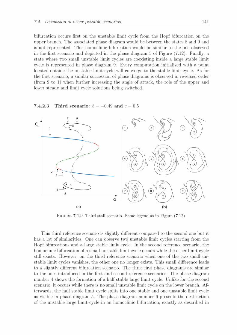
7.4. Discussion of other possible scenarios 141
bifurcation occurs first on the unstable limit cycle from the Hopf bifurcation on theupper branch. The associated phase diagram would be between the states 8 and 9 andis not represented. This homoclinic bifurcation would be similar to the one observedin the first scenario and depicted in the phase diagram 5 of Figure (7.12). Finally, astate where two small unstable limit cycles are coexisting inside a large stable limitcycle is represented in phase diagram 9. Every computation initialized with a pointlocated outside the unstable limit cycle will converge to the stable limit cycle. As forthe first scenario, a similar succession of phase diagrams is observed in reversed order(from 9 to 1) when further increasing the angle of attack, the role of the upper andlower steady and limit cycle solutions being switched.
7.4.2.3 Third scenario: b = −0.49 and c = 0.5
987
654
321
α
1
2
3
4
6
5
7
8
9
CL
(a) (b)
Figure 7.14: Third stall scenario. Same legend as in Figure (7.12).
This third reference scenario is slightly different compared to the second one but ithas a lot of similarities. One can observe two unstable limit cycles starting from theHopf bifurcations and a large stable limit cycle. In the second reference scenario, thehomoclinic bifurcation of a small unstable limit cycle occurs while the other limit cyclestill exists. However, on the third reference scenario when one of the two small un-stable limit cycles vanishes, the other one no longer exists. This small difference leadsto a slightly different bifurcation scenario. The three first phase diagrams are similarto the ones introduced in the first and second reference scenarios. The phase diagramnumber 4 shows the formation of a half stable large limit cycle. Unlike for the secondscenario, it occurs while there is no small unstable limit cycle on the lower branch. Af-terwards, the half stable limit cycle splits into one stable and one unstable limit cycleas visible in phase diagram 5. The phase diagram number 6 presents the destructionof the unstable large limit cycle in an homoclinic bifurcation, exactly as described in

142 Chapter 7. A static stall model based on the linear analysis of RANS solutions
the second reference scenario. In the phase diagram number 7, the only limit cycleexisting is the large stable limit cycle. Temporal computations can either converge tothe stable limit cycle or to the stable solution on the upper branch. Afterwards, anhomoclinic bifurcation occurs on the small limit cycle from the Hopf bifurcation on theupper branch as shown in the phase diagram number 8. Finally, the phase diagramnumber 9 is similar to the one introduced in the second reference scenario. As for theprevious scenarios, a similar succession of phase diagrams is observed in reversed order(from 9 to 1) when further increasing the angle of attack, the role of the upper andlower steady and limit cycle solutions being switched.
7.4.2.4 Fourth scenario: b = −0.42 and c = 1
α
987
654
3211
2
3
45
6
7 98
CL
(a) (b)
Figure 7.15: Fourth stall scenario. Same legend as in Figure (7.12).
The fourth reference scenario is only briefly discussed as it is simply a combinationof the second and third reference scenarios and all the phase diagrams presented in thefourth scenario are described in details in the previous cases. On can observe that thesmall limit cycles behave as in the second reference scenario and the large limit cycleis similar to the one observed in the third reference scenario.
7.4.2.5 Fifth scenario: b = −0.52 and c = 1
One shall note that the value of b used for this scenario b = −0.52 is slightly out ofthe range of recommended values for b defined in appendix E. However, this scenariois introduced as very helpful to understand the behavior of the calibrated model. Thefifth reference scenario exhibits a different behavior in the sense that no homoclinic bi-furcation occurs. However, there are still some similarities with the previous scenarios:

7.4. Discussion of other possible scenarios 143
the existence of a large stable limit cycle, unstable limit cycles from the Hopf bifur-cations and limit cycle bifurcations. Reading the bifurcation diagram in Figure (7.16)from left to right, one can first observe one unsteady stable solution represented in thephase diagram number 1. It is similar to the first state of all the reference scenariospreviously described. The phase diagram 2 shows the existence of a marginally stablelimit cycle which results from the sub-critical Hopf bifurcation on the upper branchof steady solutions. By increasing α, the half-stable limit cycle splits into two limitcycles visible in phase diagram 3. The small limit cycle centered around the uppersteady solution is unstable while the large limit cycle surrounding the upper and lowersteady solutions is stable. In phase diagram 4 these two limit cycles still exist and twounstable steady solutions have appeared on the middle and lower branches. A time-stepping computation initialized with a solution located outside of the unstable limitcycle will necessarily converges to the large limit cycle. The phase diagram 5 is similarto the phase diagram 4 except that steady unstable eigenvalue of the steady solutionon the lower branch gets unsteady, which implies that the temporal solution are noworbiting around it. Finally, the phase diagram 6 is similar to the last phase diagram ofthe second, third and fourth scenarios. Two unstable limit cycles surround two stablesteady solutions, and are separated by an unstable steady solution. All these solutionsare surrounded by a large stable limit cycle.
654
321
α
CL
(a) (b)
1
2
3
4
6
5
Figure 7.16: Fifth stall scenario. Same legend as in Figure (7.12).
7.4.2.6 Synthesis on the reference scenarios
With the range of parameters used (see equation (E.27)), at least five notable bifur-cation scenarios can be encountered depending on the value of parameters b and c.Although all different, these scenarios have a lot of common points. First, in everyscenario, the Hopf bifurcations give birth to unstable limit cycles. The main difference

144 Chapter 7. A static stall model based on the linear analysis of RANS solutions
between all these scenarios is the position at which these unstable small limit cyclescollide with the steady solution on the middle branch in a homoclinic bifurcation. Ifthe unstable limit cycles vanishes before overlapping, no other limit cycle is encoun-tered (First reference scenario). However, if the limit cycles overlap it gives birth to alarge stable limit cycle and two family of reference cases are to be distinguished: whenthe unstable limit cycles collide with the middle branch and when they do not. Thefirst family includes the second, third and fourth scenarios, which are slightly differentbut are built the same way: the small unstable limit cycle vanishes in a homoclinicbifurcation and the large stable limit cycle bifurcates in an unstable large limit cyclethat also vanishes in a homoclinic bifurcation. In the second family, correspondingto the fifth reference scenario, the unstable limit cycle never collides with the middlebranch and simply just grow until bifurcating into a stable limit cycle which surroundsall three steady solutions.
Based on these observations, one can conclude that the nonlinear behavior is dic-tated by the position of the Hopf bifurcation and the slope of the unstable limit cyclesemerging from the Hopf bifurcations. Indeed, these two characteristics will drive theexistence and, if so, the position of the homoclinic bifurcations of the small unstablelimit cycles. It was demonstrated in the previous section E.2.4 that the parameterb is directly responsible for the position of the Hopf bifurcations. The study of thereference cases also revealed that the parameter c is, at first order, responsible for theslope of the unstable limit cycle and the position of the limit cycle bifurcations (thiscan be observed by comparing the first, second and fourth scenario, which have thesame positions of Hopf bifurcation (b = −0.42) but different positions of homoclinicbifurcations due to the variation of slope of the unstable limit cycles). Finally, withthese reference scenarios, we have a better understanding on the possible formationand destruction of a large stable limit cycle.
7.4.3 Study of the nonlinear behavior in the case without hys-teresis
The study of the one-equation static stall model was performed by setting the param-eter d = −1. It ensured the presence of an hysteresis of the steady solutions. Fivedifferent scenarios were identified by modifying the parameters b and c. Among thosefive scenarios, four revealed a large stable limit cycle. Several papers in the literaturerevealed the presence of Low Frequency Oscillations (to which this limit cycle is asso-ciated) for airfoils and aerodynamic conditions which did not generate hysteresis of thesteady or mean solutions. A very interesting point is to investigate whether or not theappearance of the large limit cycle identified with unsteady RANS computations andreproduced in the static stall model is linked to the hysteresis of the steady solutions. Itappears that by switching the parameter d to a positive value, the stall phenomenon isstill modeled but the hysteresis phenomenon disappears. First, the new linear behaviorof the steady solutions along the curve is described. Then, the nonlinear behavior andthe associated scenarios are introduced.
The schematized linear behavior of the steady solutions is depicted in Figure (7.17),which exhibits, a schematized polar curve zoomed in close to the stall angle (a) and

7.4. Discussion of other possible scenarios 145
CL
α
H
H
1
2
1
(a) (b)
ω
σ
1
ω
σ
2
ω
σ
H
Figure 7.17: (a) Schematized evolution of the lift coefficient as a func-tion of the angle of attack. (b) Associated schematized temporal behaviorof the leading mode in the complex plane. The color code is similar tothe one used in Figure (5.14) of chapter 5: on the polar curve, state 1plotted in full blue line represents a stable (σ < 0) unsteady (ω = 0)eigenvalue for the associated steady solutions and state 2 plotted in fullblue line represents an unstable (σ > 0) unsteady (ω = 0) eigenvalue for
the associated steady solutions.
schematized representations of the eigenvalues in the complex planes (σ,ω), respec-tively growth rate σ and angular frequency ω of the eigenvalue λ (b). Two differentstates, numbered 1 and 2 are identified. In between, two Hopf bifurcations labelledH exist: one occurring for high lift values and the other for low lift values similarlyto the case d = −1. However, this is the only common point as this case is muchsimpler and does not exhibit saddle-node bifurcations or switch between steady andunsteady eigenvalues. Starting from the upper branch and following the polar curve,a stable unsteady eigenvalue and its complex conjugate are first encountered (state 1).As the drop of lift gets closer, these eigenvalues become less stable as their growth ratesincreases. They finally become unstable (state 2), leading to a Hopf bifurcation at thepoint noted H on the polar curve.
An approach similar to the one performed for d = −1 is repeated and several valuesof b and c are tested. Two different scenarios are identified and depicted in Figure(7.18). It exhibits two schemas of the steady states made of colored lines in the plane(cl, α) and corresponding to the the sixth scenario (a) and the seventh scenario (b).The extreme values of the limit cycles are represented in black lines. Schemas of phasediagrams are plotted for different values of α in (c). Each phase diagram is representedin the plane (dcl
dt, cl), similarly to what was done in section 7.4.2.

146 Chapter 7. A static stall model based on the linear analysis of RANS solutions
4321
α α
1
2
3
41
4
CL
(a) (b)
CL
(c)
Figure 7.18: Sixth and seventh stall scenarios. (a) and (b) Schematicbifurcation diagram including steady solutions (in colored lines) andextreme values of limit cycles (black lines) in the plane (cl, α). (c)Schematic phase diagrams in the plane (cl, cl) for different values of αreferenced on the bifurcation diagram. The color code used is similar to
the one used in Figure (7.12). .
The main difference between the two cases is the type of Hopf bifurcation : super-critical for the sixth scenario and subcritical for the seventh scenario. It appears thatthe type of the bifurcation is driven by the position of the Hopf bifurcation: if the Hopfbifurcations are inside the two points of maximum curvature, they are supercritical,otherwise, they are subcritical. For the sixth scenario (top left picture of Figure (7.18)),reading the bifurcation diagram from left to right, one can observe one unsteady stablesolution represented in the phase diagram number 1. Then, by increasing the value ofα, a supercritical Hopf bifurcation is reached. This bifurcation generates a stable limitcycle that surrounds the unstable solution. This state is presented in the phase diagramnumber 4 in which every solution will converge to this stable limit cycle. Then, as forthe previous scenarios, a similar succession of phase diagrams is observed in reversedorder (4 and 1) when further increasing the angle of attack, the bifurcations beingreversed. For the seventh scenario (top right picture of Figure (7.18)), the behavior isthe same than the sixth scenario for the states represented in phase diagrams 1 and 4.However, due to the subcriticaliity of the Hopf bifurcation, two new states presentedin phase diagrams 2 and 3 appear in between. Reading the bifurcation diagram fromleft to right, one can observe one unsteady stable solution represented in the phasediagram number 1. Then, by increasing the value of α, one encounters a limit cyclebifurcation presented in phase diagram 2. At this point, all the computations convergeto the stable solution. From this point, one unstable limit cycle and one stable limitcycle coexist as shown in the phase diagram number 3. The size of the unstable limitcycle will reduce until is vanishes at the Hopf bifurcation point while the stable limit

7.5. Conclusion 147
cycle will grow as α is increased. Then, the same behavior is repeated backwards. Inthe end, the model such as defined tends to indicate that the appearance of a largelimit cycle is not linked to the presence of an hysteresis of the steady solutions.
7.5 ConclusionIn this chapter, it was demonstrated how the static stall model (introduced in appendixE) can be calibrated to reproduce the steady states and linear behavior of the stallof an OA209 airfoil at Re = 1.8 × 10⁶ and M = 0.16 computed with the Spalart–Allmaras turbulence model. Moreover the nonlinear behavior of this model appearsto be in excellent agreement with the results of the unsteady RANS computations.Consequently, the capacity of the static stall model to reach unstable limit cycles is usedto determine a bifurcation scenario, which provide answers for all the questions raisedby unsteady RANS computations (chapter 6). Furthermore, a parametric study of thesimplest form of the static stall model (i.e. before calibration), introduced in equation(7.13) in chapter E, is conducted. Different reference scenarios are identified by varyingthe parameters of the model and it appears that the results of the calibrated model area combination of several of those reference scenarios. It remains to be seen whetherthose different scenarios would be realistic for other airfoils and flow configurations. Inthis spirit, the next chapter proposes to investigate a different Reynolds number anda different airfoil with an approach similar to the one described in chapters 5, 6 and 7and verify if different bifurcation scenarios are obtained.


149
Chapter 8
Discussion of the possible scenariosobserved
Contents8.1 Influence of the Reynolds number on the stall of an OA209
airfoil . . . . . . . . . . . . . . . . . . . . . . . . . . . . . . . . 150
8.1.1 Steady solutions . . . . . . . . . . . . . . . . . . . . . . . . . 150
8.1.2 Linear stability analysis . . . . . . . . . . . . . . . . . . . . . 151
8.1.3 Unsteady RANS computations . . . . . . . . . . . . . . . . . 152
8.1.4 Application of the one-equation static stall model to the casewithout hysteresis . . . . . . . . . . . . . . . . . . . . . . . . 154
8.1.5 Comparison of the cases at Re = 1.8× 10⁶ and Re = 0.5× 10⁶ 156
8.2 Investigation of the stall for a NACA0012 airfoil . . . . . . 157
8.2.1 Literature review and motivations . . . . . . . . . . . . . . . 157
8.2.2 Results with the Spalart–Allmaras model . . . . . . . . . . . 161
8.2.3 Results with the Edwards–Chandra modification . . . . . . . 165
8.2.4 Discussion of the case of the NACA0012 at Re = 1.0× 10⁶ . . 168
8.3 Conclusion . . . . . . . . . . . . . . . . . . . . . . . . . . . . . 169
In this chapter, two additional configurations are presented. The objective is to verifyif a bifurcation scenario similar to the one described in section 7.2 can be identifiedand, if not, if the reference scenarios detailed in section 7.4 are representative of theconfigurations presented. At first, the case of an OA209 airfoil at a lower Reynoldsnumber Re = 0.5 × 10⁶ is presented (the case Re = 1.0 × 10⁶ is also investigatedbut, as it reveals a scenario strictly similar to the one presented in chapters 5 to 7,it is just briefly introduced). Then, a different airfoil is tested : a NACA0012 atRe = 1.0 × 10⁶. This choice of configuration is motivated by the numerical study ofWales et al. [166] and the experimental study of Hristov and Ansell [70]. For thiscase, the whole approach could not be carried out due to a lack of time. However, theavailable data reveal a similar behavior, although more complex. Finally, the resultsobtained in these different configurations are compared to the case of the OA209 airfoilat Reynolds number Re = 1.8× 10⁶.

150 Chapter 8. Discussion of the possible scenarios observed
8.1 Influence of the Reynolds number on the stall ofan OA209 airfoil
Two computations are performed for an OA209 airfoil at different Reynolds numbers:Re = 1.0 × 10⁶ and Re = 0.5 × 10⁶. These values are intentionally high enoughto ensure that the RANS approach, considering a fully turbulent boundary layer, isstill pertinent and the solutions are still meaningful from a physical point of view.The method used is similar to the one performed and presented through the differentchapters: first the steady solutions are computed using continuation methods, secondthe stability analysis of each solution is performed and finally a bifurcation scenario isdeduced fromunsteady RANS computations and the static stall model.
8.1.1 Steady solutions
The polar curves of the lift coefficient corresponding to the two additional values ofReynolds number tested are plotted with the polar curve of the case at Re = 1.8×10⁶ inFigure (8.1). In Figure (8.1)(a), which presents the three polar curves, one can observehow an increase of the Reynolds number (direction of the black arrow) increases themaximum lift coefficient value and the stall angle. Moreover, in Figures (8.1)(b), (c)and (d), which present zooms close to stall for the three cases, one can also observe howit affects the appearance of the hysteresis area close to stall: for the smallest Reynoldsnumber, no hysteresis is identified and for the two others, the higher the Reynoldsnumber, the larger the range of coexisting solutions.
CL
14 16 18 20
1
1.2
1.4
1.6
bc
d
16.95 17 17.05 17.11
1.2 (b)
(a)18.37 18.42 18.47 18.52
1.2
1.4
α(°)α(°)
(d)
CL
17.75 17.8 17.85 17.91.2
1.4(c)
Figure 8.1: (a) Evolution of the lift coefficient as a function of the angleof attack for the flow around an OA209 airfoil at Mach number M = 0.16and for three different Reynolds numbers: Re = 0.5 × 10⁶ (labelled b),Re = 1.0 × 10⁶ (labelled c) and Re = 1.8 × 10⁶ (labelled d). (b), (c)and (d): zooms on the polar curves close to stall for Re = 0.5 × 10⁶,Re = 1.0 × 10⁶ and Re = 1.8 × 10⁶ respectively (letters matching the
ones used in (a)).

8.1. Influence of the Reynolds number on the stall of an OA209 airfoil 151
The flow topology of the steady solutions is similar to the one presented in Figure(5.1) of section 5.1 for the three cases tested: a recirculation bubble appears at thetrailing edge for low angles of attack and the separation point moves toward the trailingedge as the angle of attack increases.
8.1.2 Linear stability analysis
This section is dedicated to the stability of steady solutions obtained for Re = 0.5×10⁶
for which no hysteresis is observed when varying the angle of attack (the results ob-tained for Re = 1.0×10⁶ exhibit a scenario similar to the one obtained for Re = 1.8×10⁶
and described in section 5.2). Similarly to the case Re = 1.8× 10⁶, two complex eigen-modes are found unstable in the explored range of angles of attack. A low-frequencystall eigenmode is unstable in a small range of angles of attack where the lift coefficientdrops suddenly. A high-frequency vortex-shedding eigenmode becomes unstable forhigher angles of attack α > 19.50◦, in the post-stall regime. The temporal features andthe structures of these modes are similar to the ones described in sections 5.2.3 and5.2.4.1 respectively for the case at Reynolds number Re = 1.8 × 10⁶. As a reminder,the vortex shedding mode, existing for high angles of attack, when the flow is detached,has a Strouhal number St ≈ 0.2. The topology of this mode, which is made of largestructures convected upward, is represented in Figures (5.6)(b) and (d) of chapter 5.The stall mode, has a lower Strouhal number St ≈ 0.05. The topology of this mode,which is made of a large pulsating structure located on the suction side of the airfoil,is depicted in Figures (5.6)(a) and (c). The main difference for the case at Reynoldsnumber Re = 0.5× .106 is the evolution of the low frequency mode as a function of theangle of attack.
α (°)
CL
16.6 16.8 17 17.2 17.4
1.2
1.4s
1
2
1
σ
ω
-0.02 0 0.02-0.04
0
0.04
(a) (b)
Figure 8.2: Real evolution of the temporal behavior of the leadingmode. (a) polar curve zoomed in close to stall and associated temporalbehavior. (b) Superimposition of the spectra obtained from each steadysolution along the polar curve (the black arrows indicate the direction ofan increasing curvilinear abscissa). The color code is similar to the oneof Figure (7.17) in chapter 7. The grey area corresponds to the zone in
which the modes are unstable.

152 Chapter 8. Discussion of the possible scenarios observed
Figure (8.2) shows a superposition of all the eigenspectra (b) computed for angles ofattack in the range 12.00◦ ≤ α ≤ 17.30◦ (a). The displacement of the leading complexeigenvalues (blue points) in the plane (σ, ω) clearly shows that they get first unstable(dashed line on the polar curve and grey area in the complex plan) when increasingthe angle of attack above α = 16.95◦ and then get stable for α ≥ 17.08◦. The identifi-cation of the unstable region 16.95◦ ≤ α ≤ 17.08◦ is clear when examining the growthrate as a function of the angle of attack displayed in Figure (8.3) (a). The change ofslope for the growth rate occurs around α = 16.98◦ and is associated to an increaseof the frequency, as seen in Figure (8.3) (b). The angular frequency ω = 0.015 at thesecond Hopf bifurcation is slightly larger than ω = 0.026, the angular frequency at thefirst Hopf bifurcation. Note that this scenario is in perfect agreement with the onepredicted by the model in the case without hysteresis (parameter d of the model set tod = 1) and whose a schematized representation is proposed in Figure (7.17) of chapter 7.
α (°)
σ
16.4 16.8 17.2
-0.01
0
ω
16.4 16.8 17.2
-0.04
0
0.04
α (°)
(a) (b)
Figure 8.3: Evolution of the angular frequency (a) and the growth rate(b) as a function of the angle of incidence. The direction of the arrows
refers to increasing curvilinear abscissa.
8.1.3 Unsteady RANS computations
As identified in section 4.3.1, a difference between the solutions obtained with con-tinuation methods and local time stepping methods exists. A solution is proposed inappendix C and validated in appendix D and chapter 6. It consists in slightly modify-ing the cutoff value on the turbulent variable and allows us to obtain a good agreementbetween the linear stability of steady solutions obtained with continuation methodsand unsteady RANS computations. For the case Re = 0.5× 10⁶, the unsteady RANScomputations were actually performed before identifying the modification of the cutoffas a solution to reconcile RANS computations and continuation methods. In order toavoid performing additional time costly unsteady RANS computations, it was decidedto live with the small shift between the two approaches. It was verified for a few steadysolutions that the stability analysis is qualitatively similar in both cases. Consequently,the results of the unsteady RANS computations presented in Figure (8.4) are slightly

8.1. Influence of the Reynolds number on the stall of an OA209 airfoil 153
shifted compared to the bifurcation scenario calibrated on the steady states from con-tinuation methods and their linear behavior (presented in Figure (8.5)).
α(° )
CL
16.85 16.9 16.95 171
1.1
1.2
1.3
1.4
(a) (b)
Time
CL
0 2000 4000 6000
1.1
1.2
1.3
1.4
Figure 8.4: Results of the unsteady RANS computations. (a) Timeevolution of the lift coefficient for an angle of attack of α = 16.91◦. Com-putation initialized with a steady solution at the same angle of attack.(b) Evolution of the lift coefficient for the steady states (full black linesand dashed black line) and visualisation of the extreme values of thelimit cycle (full red lines). The linear behavior of the steady states isindicated by a dashed line for the linearly unstable ones and by a full
line for the linearly stable ones.
Figure (8.4)(a) shows the evolution of the lift coefficient as a function of the timefor the particular case of α = 16.91◦. This curve is obtained from an unsteady RANScomputation initialized with the steady solution at the same angle of attack. For thisangle of attack the linear stability analysis of the steady solution revealed an unsteadyunstable mode. The lift coefficient fast diverges from the lift value of the steady state.It oscillates until it reaches a limit cycle of large amplitude (ΔCL ≈ 0.3). The analysisof the structure of the unsteadiness reveals a recirculation bubble pulsating from thetrailing edge, which is similar to the mechanism presented in Figure (6.2) in chapter 6for the case at higher Reynolds number. It generates a high lift state (corresponding tothe maximum value of the limit cycle) when the recirculation bubble is tiny and locatedat the trailing edge and a low lift state (corresponding the minimum value of the limitcycle) when the recirculation bubble is large and extends on the whole suction side.The Strouhal number associated with this unsteady phenomenon is St = 0.00545. Sucha value is two orders of magnitude lower than the classic bluff body vortex sheddingStrouhal number St ≈ 0.2 and in good agreement with the Strouhal number of theunstable mode identified with the linear stability analysis St = 0.00296. All these ob-servations (large amplitude oscillations at a low Strouhal number and structure madeof a pulsating recirculation bubble on the suction side of the airfoil) tend to indicatethat this phenomenon is similar to the one observe at higher Reynolds number whenthere is an hysteresis (presented in chapter 6) and described in the literature as lowfrequency oscillations (see section 1.3.2). The study of the possible different scenarios

154 Chapter 8. Discussion of the possible scenarios observed
with the static stall model showed that the appearance of such a limit cycle was con-ditioned by the positions of the Hopf bifurcations and the position of the intersectionof the unstable limit cycle with the middle branch of steady solutions. Thus, it wassupposed that the Hopf bifurcations played a more significant role in the formation ofthis limit cycle than the saddle-node bifurcations. This case confirms this hypothesisand, even more, highlights the fact that the existence of this limit cycle of high am-plitude and low frequency is independent of the existence of saddle-node bifurcationsand a hysteresis of the steady solutions.
Limit cycle solutions have been tracked when varying the angle of attack using asimple parameter continuation (as described in chapter 6). The full red lines in Figure(8.4)(b) are the maximal and minimal values of the limit cycles obtained when varyingthe angle of attack. For comparison, the branch of steady solutions (obtained withsteady RANS computations) is reproduced in this figure with a solid (resp. dashed)curve when it is stable (resp. unstable). Interestingly, the limit cycle branch existsin the range of angle of attack 16.87◦ ≤ α ≤ 17.20◦ that is larger than the range ofinstability 16.88◦ ≤ α ≤ 17.00◦ found for the steady solutions. Consequently, the Hopfbifurcations at α = 16.88◦ and α = 17.00◦ are both sub-critical. Limit cycle solutionsthus exist for values of the angle of attack for which the steady solutions are stable,approximatively in the range 16.87◦ ≤ α ≤ 16.88◦ (resp. 17.00◦ ≤ α ≤ 17.20◦) for thefirst (resp. second) Hopf bifurcation.
8.1.4 Application of the one-equation static stall model to thecase without hysteresis
At first, one shall note that the steady states presented in subsection 8.1.1 were com-puted with continuation methods, which implies that the cutoffs on the turbulentvariable implemented into the solver are not taken into account (see section 4.3.1).The linear stability analysis presented in section 8.1.2 is based on these steady solu-tions obtained with a continuation method. However, the unsteady RANS compu-tations (presented in subsection 8.1.3) were performed with the standard version ofthe Spalart–Allmaras turbulence model in the sense of elsA, which means that sev-eral cutoffs were active. The static stall model, which requires results from the linearstability analysis, will be calibrated using results obtained with continuation methods.Consequently, it will not be possible to quantitatively compare the results from thestatic stall model and from the unsteady RANS computations. However, a qualitativecomparison will be possible and will provide interesting insights about the criticaliityof the Hopf bifurcations and the width of the limit cycle.
Section 7.4 was dedicated to the study of different scenarios based on the valuesof the one-equation static stall model. The sixth and seventh scenarios detailed insubsection 7.4.3 of chapter 7 were for cases without hysteresis of the steady solutions.As a reminder, a low frequency large amplitude limit cycle is found in the two cases.The difference between the two scenarios is the type of Hopf bifurcation, supercriticalor subcritical, which is driven by their positions. If the Hopf bifurcations are insidethe two points of maximum curvature, they are supercritical, otherwise, they are sub-critical. At first, note that the results of the linear stability analysis and the unsteady
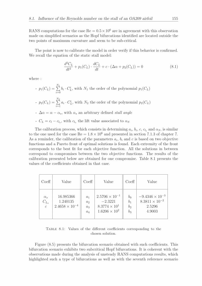
8.1. Influence of the Reynolds number on the stall of an OA209 airfoil 155
RANS computations for the case Re = 0.5×10⁶ are in agreement with this observationmade on simplified scenarios as the Hopf bifurcations identified are located outside thetwo points of maximum curvature and seem to be sub-critical.
The point is now to calibrate the model in order verify if this behavior is confirmed.We recall the equation of the static stall model:
d2CL
dt2+ p1(CL) · dCL
dt+ c · (Δα + p2(CL)) = 0 (8.1)
where :
- p1(CL) =N1∑i=0
bi · C iL, with N1 the order of the polynomial p1(CL)
- p2(CL) =N2∑i=1
ai · C iL, with N2 the order of the polynomial p2(CL)
- Δα = α− αs, with αs an arbitrary defined stall angle
- CL = cl − cls , with cls the lift value associated to αS
The calibration process, which consists in determining ai, bi, c, cls and αS, is similarto the one used for the case Re = 1.8× 10⁶ and presented in section 7.1.3 of chapter 7.As a reminder, the calibration of the parameters ai, bi and c is based on two objectivefunctions and a Pareto front of optimal solutions is found. Each extremity of the frontcorresponds to the best fit for each objective function. All the solutions in betweencorrespond to compromises between the two objective functions. The results of thecalibration presented below are obtained for one compromise. Table 8.1 presents thevalues of the coefficients obtained in that case.
Coeff Value Coeff Value Coeff Value
αs 16.985366 a1 2.5706× 10⁻¹ b0 −9.4346× 10⁻³
CLs 1.240135 a2 −2.3221 b1 8.3811× 10⁻²
c 2.4658× 10⁻⁴ a3 8.3774× 101 b2 2.5296a4 1.6206× 10² b3 4.9003
Table 8.1: Values of the different coefficients corresponding to thechosen solution.
Figure (8.5) presents the bifurcation scenario obtained with such coefficients. Thisbifurcation scenario exhibits two subcritical Hopf bifurcations. It is coherent with theobservations made during the analysis of unsteady RANS computations results, whichhighlighted such a type of bifurcations as well as with the seventh reference scenario

156 Chapter 8. Discussion of the possible scenarios observed
depicted in Figure (7.18)(b). The range of existence of the limit cycle is similar betweenthe static stall model (≈ 0.12◦) and the unsteady RANS computations (≈ 0.16◦). Themodel slightly underestimates the range of existence of the limit cycle, similarly towhat was observed for the case at Re = 1.8× 10⁶. Finally, the similarities between thestatic stall model and the unsteady RANS computations prove that the model, whichwas created based on a hysteresis behavior, successfully reproduces the nonlinear be-havior observed when there is no hysteresis.
1
1.05
1.1
1.15
1.2
1.25
1.3
1.35
1.4
16.92 16.94 16.96 16.98 17.00 17.02 17.04 17.06 17.08 17.10
CL
α (°)
Figure 8.5: Bifurcation diagram of the model calibrated on the linearbehavior observed during RANS computations. The color code is similarto the one of Figure (7.5). The steady solutions are plotted in blue andthe black lines represent the extreme values of the surrounding limitcycle. The unstable solutions are plotted with dashed lines while the
stable ones are associated to full lines.
8.1.5 Comparison of the cases at Re = 1.8×10⁶ and Re = 0.5×10⁶
It is interesting to compare this scenario with the one described in chapter 5. Atfirst sight, they might seem very different as this one is much simpler. However, theirbehaviors are strongly linked. They both start with an unsteady stable mode thatbecomes unstable and less unsteady at the same time. The only difference is that, inthe case with hysteresis, the angular frequency decreases enough to become null. Whenit happens, the new unstable steady mode splits into two steady modes and when oneof these two modes becomes stable, the saddle-node bifurcation occurs. On the otherhand, in the case without hysteresis (Re = 0.5 × 10⁶), the angular frequency of themode never becomes null and starts increasing before reaching the axis St = 0 (Figure8.2).
In the end the complete scenario makes sense: there is an unsteady mode respon-sible for stall that becomes unstable around the stall angle. The complexity of the

8.2. Investigation of the stall for a NACA0012 airfoil 157
scenario depends on the temporal behavior of this mode: a saddle-node occurs whena steady mode crosses the axis σ = 0. When there is no hysteresis, and consequentlyno saddle-node bifurcation, the unsteady mode never becomes steady whereas withhysteresis, the unsteady mode becomes null and split into two steady modes, whichmight lead to a saddle-node bifurcation.
The model originally created for the most complicated case with a hysteresis isactually robust and works well without extra efforts for the simplest case withouthysteresis. The study of this model reveals that both cases generate low frequencyoscillations around the stall angle even though the appearance and disappearance ofthe limit cycle in the case with hysteresis is more complicated. These observations areconfirmed with unsteady RANS computations for the two scenarios.
Finally, one shall note that an attempt to link the evolution of hysteresis as afunction of the Reynolds number from a bifurcation theory point of view was proposedby Cui et al. [34]. A similar approach could be very useful to identify the criticalReynolds number for which hysteresis disappears and could provide very interestinginsight on how the limit cycles evolve from the case with hysteresis to the case withoutand, particularly, close to the critical point.
8.2 Investigation of the stall for a NACA0012 airfoilThe bifurcation scenario of a NACA0012 at Reynolds number Re = 1.0× 10⁶ is inves-tigated. First, several results that can be found in the literature are introduced. Thepossibility to compare as much as possible to these results is the main motivation thathave led to the choice of this configuration. Afterwards, the steady solutions obtainedwith continuation methods and their linear stability are introduced. Two differentcases are actually investigated for this configuration: one with the Spalart–Allmarasmodel and one with a modified version of the Spalart–Allmaras model [46]. This choiceis motivated by the aforementioned literature review. Due to a lack of time, the nonlinear behavior could not be investigated for this airfoil.
8.2.1 Literature review and motivations
In a recent paper, Hristov and Ansell [70] investigated experimentally the static stallphenomenon around the symmetric NACA0012 airfoil at the Reynolds number Re =1.0 × 10⁶. The polar curves obtained by Hristov and Ansell are presented in Figure(8.6), which exhibits the evolution of the lift (a) and the pitching moment (b) as afunction of the angle of attack. One can identify two branches in the area where thelift coefficient decreases : the blue one is obtained by increasing α while the red one isobtained by decreasing α. The existence of two solutions based on the history of theflow is characteristic of a hysteresis phenomenon. However, note that in the presentcase, these lift coefficient values are time-averaged while the hysteresis described in thismanuscript for the OA209 is obtained from steady lift values. The hysteresis identifiedby Hristov and Ansell implies different limit cycles for the two branches.

158 Chapter 8. Discussion of the possible scenarios observed
[deg]
Cl
-5 0 5 10 15 20 25-0.5
0
0.5
1
1.5
Upstroke
Downstroke
Increasing
Decreasing α
α
α
[deg]
Cm
-5 0 5 10 15 20 25-0.15
-0.1
-0.05
0
0.05
Increasing
Decreasing
α
α
α
(a) (b)
Figure 8.6: Evolution of the lift coefficient (a) and the pitching moment(b) for several angles of attack for a NACA0012 at Re = 1.0× 10⁶ from
Hristov and Ansell [70].
They also measured the unsteady surface pressure and, from it, deduced the Strouhalnumber1 of the phenomena involved. Figure (8.7) presents a map of the Strouhal num-ber as a function of the position on the airfoil (made nondimensional with the chord c.).Three angles of attack are investigated for each solution of the hysteresis: α = 14.00◦
(a) and (d), α = 15.00◦ (b) and (e) and α = 16.00◦ (c) and (f). The high lift solutions(labelled upstroke in the legend of Figure (8.6)) are on the left (a), (b) and (c) andthe low lift solutions (labelled downstroke in the legend of Figure (8.6)) are on theright (e), (f) and (g). From this spectral analysis, one can observe two very distinctphenomena: one of very low Strouhal number St ≈ 0.01 of large amplitude near theleading edge (0 ≤ x/c ≤ 0.2) and one of Strouhal number St ≈ 0.2 of large amplitudemore upstream (0.2 ≤ x/c ≤ 0.9). Hristov and Ansell describe the unsteadiness closeto the leading edge as a low frequency oscillations mechanism as its Strouhal numberand location are in good agreement with the studies more extensively presented insection 1.3.2. Also, they argued that the Strouhal number of the higher frequency phe-nomenon observed downstream is in agreement with classic bluff-body shedding suchas the one identified by Roshko [142]. With time resolved particle image velocimetry(not presented here but visible in detail in the PhD of Hristov [69]) they confirmed thatthe low frequency phenomenon is a movement of the separation point characteristicof the LFO described in the literature. However, one should note that the amplitudeof the separation point displacement is quite small (≈ 15% of the chord) compared tothe displacement of the separation point encountered in this study (Figure (6.2)) or inthe literature (Figure (1.9) from Broeren [23]). The difference between these studiesand the one of Hristov seems to be the simultaneous existence of a vortex sheddingunsteadiness and low frequency oscillations. Finally, the amplitude of these phenom-ena evolves with the angle of attack as illustrated in Figure (8.7): the upper branch ismostly dominated by the low frequency unsteadiness (the vortex shedding mechanism
1Based on the chord length weighted by the sine of the angle of attack: St = f ·c·sin(α)U∞

8.2. Investigation of the stall for a NACA0012 airfoil 159
Figure 8.7: Maps representing the Strouhal number of unsteady phe-nomena as a function of their position along the suction side of the airfoil.On the upper branch : α = 14.00◦ (a), α = 15.00◦ (b) and α = 16.00◦
(c). On the lower branch : α = 14.00◦ (d), α = 15.00◦ (e) and α = 16.00◦
(f). From Hristov and Ansell [70].
is also identified but is very weak). On the contrary, the lower branch is driven by thevortex shedding phenomenon mostly, even if one can notice that for α = 14.00◦, both

160 Chapter 8. Discussion of the possible scenarios observed
phenomena seem to coexist. In the end, Hristov and Ansell observed the followingregarding the unsteady mechanisms in the hysteresis area:
- The low frequency oscillations are dominant at the end of each branch (Figures(8.7)(b), (c) and (d))
- The vortex shedding mechanism is dominant at the end of the lower branch(Figures (8.7)(d) and (e)). On this branch, the amplitude of this unsteadinessdecreases as the angle of attack increases
- The two phenomena coexist for α = 14.00◦ on the lower branch (Figure (8.7)(d))
Several numerical studies on a NACA0012 at high Reynolds number can also befound in the literature. Mittal [110] identified a hysteresis between 17.00◦ < α < 19.00◦
with unsteady RANS computations coupled with the Baldwin-Lomax turbulence modelat Reynolds number Re = 1.0 × 10⁶. Although the stall angle is higher than the ex-perimental one identified by Hristov and Ansell (probably due to the limitations of theRANS modeling detailed in section 1.4), the range of hysteresis identifed by Mittal[110] matches the one of Hristov and Ansell [70]. Wales et al. [166] conducted a nu-merical study that consisted in computing steady solutions with continuation methodsfor a flow at high Reynolds number (Re ≥ 1.85× 10⁶). Particularly, they investigatedthe influence of the Edwards–Chandra modification of the Spalart–Allmaras model[46] (this modification is introduced in section 2.1.4) and the influence of the turbulentvariable boundary condition. Figure (8.8) exhibits the steady solutions obtained forfour different cases : with two values of the boundary condition ratio
(μt
μ
)∞
(3.0 and10.0) and with/without the Edwards–Chandra modification of the Spalart–Allmarasmodel. This figure shows that the level of freestream turbulent has a direct effect onthe appearance of a hysteresis steady solutions with the Spalart–Allmaras. This ober-vation is coherent with the one made by Marchman [94] who noted that the freestreamturbulence level had an impact on the appearance of hysteresis in wind tunnel. More-over, Figure (8.8) also shows that the original Spalart–Allmaras model fails to catchhysteresis in the case of a NACA0012 while the modification proposed by Edwards andChandra [46] succeed to identify a hysteresis of steady solutions.
In the end, the NACA0012 airfoil at high Reynolds number seems to be able to com-bine simultaneously a hysteresis and low frequency oscillations [70], which are the twomain features of the bifurcation scenario identified for the OA209 airfoil at Reynoldsnumber Re = 1.8 × 10⁶. In that sense, it is the perfect candidate to investigate therobustness of the bifurcation scenario. Moreover, based on the numerical computationscarried out by Wales et al. [166], it is very likely that at Re = 1.0× 10⁶, the Spalart–Allmaras turbulence model fails to catch a hysteresis while the Edwards–Chandra mod-ification of the model might be able to. Consequently, it appears interesting to studyboth cases as it would allow us to obtain one case without hysteresis to be comparedto the scenario identified for the OA209 at Re = 0.5 × 10⁶ and one with hysteresis tobe compared to the scenario identified for the OA209 at Re = 1.8 × 10⁶. It must benoted that contrary to what is done by Wales et al. and what is presented in Figure(8.8) the boundary condition of the turbulent variable, set by the ratio μt
μwill not be
changed and will remain equal to 3.0 in agreement with the value suggested by Spalart

8.2. Investigation of the stall for a NACA0012 airfoil 161
alpha
Cl
12 14 16 18 20 22 24 26 28 30
0.6
0.8
1
1.2Spalart Allmaras Edwards 3.0Spalart Allmaras Edwards 10.0Spalart Allmaras 3.0Spalart Allmaras 10.0
Figure 8.8: Influence of the turbulent boundary condition on thesteady solutions around a NACA0012 at Mach number M = 0.3 and
Reynolds number Re = 1.85× 10⁶ from Wales et al. [166].
and Rumsey [152] and to the boundary conditions used for the OA209. Finally, a com-parison of the results with the aforementioned studies should give us insights on thevalidity of our approach and its capacity to correctly identify the phenomena observedexperimentally.
8.2.2 Results with the Spalart–Allmaras model
First, the case of the flow around a NACA0012 airfoil at Reynolds number Re =1.0× 10⁶ modelled with the original version of the Spalart–Allmaras turbulence modelis investigated. Based on the results of Wales et al., an evolution of the steady statessimilar to the one obtained with the OA209 at Re = 0.5×10⁶ is expected and a similarbifurcation scenario is supposed at first. The evolution of the lift coefficient as a func-tion of the angle of attack is presented in Figure (8.9):(a) depicts a general overview and(b) a zoom close to stall. As expected, the polar curve does not exhibit any hysteresis.Moreover, if the stall angle is overestimated compared to the experiment of Hristov andAnsell [70], the maximum lift value is in good agreement with the one they observed.This figure also presents the areas where a linearly unstable mode is identified with theglobal stability analysis: they are highlighted with dashed lines. Similarly to the casesof the OA209, two unstable modes are encountered: one low frequency mode close tostall and one of higher frequency when the flow is massively separated. The secondone, is a very classic bluff-body mode of Strouhal number St = 0.2.
Figure (8.10) presents the structure of the eigenmode: (a) depicts the real part ofthe streamwise velocity component ρu and (b) the real part of the turbulent variableρν. The structure of the low frequency mode is very similar to the structure of themode identified in the cases of the OA209 airfoil (see Figure (5.6)): the main structure

162 Chapter 8. Discussion of the possible scenarios observed
0.8
1
1.2
1.4
α(° )
CL
14 16 18 20 22 17.6 18 18.4
1
1.2
α(° )
CL
(a) (b)
Stall
mode
Vortex
shedding
mode
Stall
mode
Figure 8.9: Evolution of the lift coefficient as a function of the angleof attack for an NACA0012 airfoil at Re = 1.0 × 10⁶ and M = 0.16with a RANS approach coupled with the original version of the Spalart–Allmaras turbulence model. (a) Full polar curve. (b) Zoom close to stallangle. Dashed lines indicate the solutions for which an unstable mode is
encountered.
is located just above the recirculation bubble. However, in the case of the NACA0012,the flow seems to be more massively separated and consequently, the main structureof the mode is located more upstream than in the case of the OA209.
a) b)
(a) (b)
Figure 8.10: Visualisation of the structure of the eigenmodes. (a) Realpart of the ρu field of the stall eigenmode (α = 18.05◦). (b) Real part of
the ρν field of the stall eigenmode (α = 18.05◦).
Then, the evolution of the eigenmode along the polar curve is investigated. Thesuperimposition of the spectra is presented in Figure (8.11): (a) shows the evolution ofthe lift coefficient as a function of the angle of attack (the areas where an unstable modeis found are highlighted by dashed lines) and (b) the superimposition of the spectracomputed for every angle of attack (only the stall mode, introduced in Figure (8.10),is represented). At first sight, the evolution seems different from the one observed forthe OA209 airfoil at Reynolds number Re = 0.5× 10⁶ and for which a schematic rep-resentation of this behavior is represented in Figure (7.17). However, close to stall, thebehavior is actually very similar (for 17.90◦ < α < 18.20 in the (α,CL) plane and forω < 0.05 in the complex plane (σ, ω)). Indeed, starting from the most left blue dots,which correspond to the stall mode and its complex conjugate obtained for α = 12.00◦,

8.2. Investigation of the stall for a NACA0012 airfoil 163
as the angle of attack increases, this mode becomes less and less stable until it finallybecomes unstable. Then, while its angular frequency increases, the mode is stabilizedagain. So far, the evolution is indeed identical to the one described in section 8.1.2for the OA209 at Reynolds number Re = 0.5 × 10⁶. The main difference appears forhigher angles of attack (α > 19.20◦ in the (α,CL) plane and ω > 0.05 in the complexplane (σ, ω)): instead of staying stable, the mode describes a Z shape and becomesunstable again for a very few angles of attack before finally getting stable while itsangular frequency increases.
α(°)
CL
17 18 19 20
0.8
1
1.2
1.4
σ
ω
-0.01 0
-0.1
0
0.1
(a) (b)
s
Figure 8.11: Real evolution of the temporal behavior of the leadingmode in the case of a NACA0012 at Re = 1.0 × 10⁶ with the originalSpalart–Allmaras model. (a) Polar curve zoomed in close to stall and as-sociated temporal behavior. (b) Superimposition of the spectra obtainedfrom each steady solution along the polar curve. Color code similar asthe one of Figure (5.13). The grey area corresponds to the zone in which
the modes are unstable.
To have a better understanding of the origins of this particular Z shape, the evolu-tion of the angular frequency and of the growth rate are studied in more detail for thetwo unstable modes (stall mode and vortex shedding mode) . The evolutions of the an-gular frequencies as a function of the angle of attack are depicted in Figures (8.12)(a)and (c) and the evolutions of the growth rates as a function of the angle of attackare depicted in Figures (8.12)(b) and (d). Focusing on the evolution of the growthrate of the stall mode, one can observe on the first part of the curve (α < 18.50◦) abehavior similar to the one of the OA209 airfoil at Reynolds number Re = 0.5 × 10⁶
(presented in Figure (8.3)). For larger angles of attack (α ≥ 18.50◦), the growth rateof the stall mode increases again and event gets unstable in a narrow range of angle19.20◦ ≤ α ≤ 19.40◦ with a peak for α = 19.30◦. Examining the growth rate of thevortex-shedding eigenmode depicted in Figure (8.12)(d), it appears that this mode be-comes unstable for the angle of attack α = 19.30◦ corresponding to the peak of growthrate of the stall mode during the second destabilization (this value is marked by dashedline linking Figures (8.12)(b) and (d)). Also, the angle of attack for which the vortexshedding mode becomes unstable seems to correspond to a break in the slope of the

164 Chapter 8. Discussion of the possible scenarios observed
evolution of the Strouhal number as illustrated by a dashed line in Figures (8.12)(a)and (c). Finally, note that the angle of attack for which the vortex shedding modeis first identified seems to correspond to a break of slope in the evolution of the stallmode’s growth rate (marked by dashed line linking Figures (8.12)(b) and (d)). In theend, it seems that the behavior of the stall mode is similar to the one observed forthe OA209 at Reynolds number Re = 0.5 × 10⁶ at stall but is then affected by theappearance of the vortex shedding mode which appears right after stall, for angles ofattack smaller than in the case of the OA209.
α (°)
σ
16 18 20 22
-0.01
0
α (°)
σ
16 18 20 22
-0.01
0
0.01
α (°)
ω
16 18 20 22
-0.4
0
0.4
α (°)
ω
16 18 20 22
-0.1
0
0.1
(a) (b)
(c) (d)
Figure 8.12: Evolution of the eigenvalues as a function of the angle ofattack in the case of a NACA0012 at Re = 1.0 × 10⁶ with the originalSpalart–Allmaras model. (a) and (c): evolution of the angular frequencyas a function of the angle of attack. (b) and (d): evolution of the growthrate as a function of the angle of attack. (a) and (b): stall mode. (c)
and (d): vortex shedding mode.

8.2. Investigation of the stall for a NACA0012 airfoil 165
8.2.3 Results with the Edwards–Chandra modification
Based on the results of Wales et al., it is expected that, by using the Edwards–Chandramodification of the Spalart–Allmaras turbulence model, a hysteresis of the steadysolutions could be identified for the flow around a NACA0012 at Reynolds numberRe = 1.0 × 10⁶. Such a scenario could be compared to the results obtained withoutthe modification of the turbulence model, to the results obtained for the OA209 airfoilat Re = 1.8×10⁶, and to the results of the experimental study of Hristov and Ansell [70].
The polar curve obtained with continuation methods is presented in Figure (8.13):(a) depicts the general overview of the evolution of the lift coefficient as a function ofthe angle of attack and (b) shows the same evolution zoomed in close to stall angle.As expected regarding the results obtained by Wales et al. [166] with the Edwards–Chandra modification of the Spalart–Allmaras model, a hysteresis existing for a largerange of angles of attack is identified. Note that for this airfoil, the hysteresis is muchlarger than the one found for the OA209 airfoil : ΔαHyst ≈ 2.8◦ for the NACA0012and ΔαHyst ≈ 0.1◦ for the OA209. The areas where an unstable mode is found arehighlighted with dashed lines. Similarly to the cases of the OA209 at various Reynoldsnumbers and of the NACA0012 with the original Spalart–Allmaras model, the stalleigenmode and the vortex shedding mode are encountered. The structure of the stallmode is similar to the one of the mode found for the NACA0012 with the originalSpalart–Allmaras turbulence model and presented in Figure (8.10).
14 16 18 200.6
0.8
1
1.2
1.4
α(° )
CL
17 18 19 200.6
0.8
1
1.2
1.4
α(° )
CL
(a) (b)
Stall
mode
Vortex
shedding
mode
Stall
mode
Vortex shedding mode
Figure 8.13: Evolution of the lift coefficient as a function of the angleof attack for an NACA0012 airfoil at Re = 1.0×10⁶ and M = 0.16 with aRANS approach coupled with the Edwards–Chandra modification of theSpalart–Allmaras turbulence model. (a) General overview of the polar
curve. (b) Zoom close to stall angle.
Figure (8.14)(a) shows the evolution of the lift coefficient as a function of the angleof attack (the areas where an unstable mode is found are highlighted by dashed lines)and Figure (8.14)(b) the superimposition of the spectra computed for every angle ofattack. Schematically, the behavior observed for the NACA0012 at Reynolds number

166 Chapter 8. Discussion of the possible scenarios observed
Re = 1.0× 10⁶ with the Edwards–Chandra modification of the Spalart–Allmaras tur-bulence model is very similar to the scenario depicted for the OA209 airfoil at Reynoldsnumber Re = 1.8×10⁶. The two blue dots the closest of the abscissa axis correspond toα = 12.00◦ on the upper branch, to the most left blue dots corresponding to α = 18.40◦
on the lower branch. For higher angles of attack the mode is difficult to track as itevolves quite fast and surrounded by a lot of spurious modes. More generally, thesmallest circular arc of blue dots describes the evolution on the upper branch whereasthe largest circular arc describes the evolution on the lower branch. From a globalpoint of view, the superimposition of the eigenspectra shows results mostly similar tothe case of the OA209 at Reynolds number Re = 1.8× 10⁶
α(°)
CL
17.5 18.5 19.50.6
0.8
1
1.2
1.4
σ
ω
0 0.1 0.2
-0.2
-0.1
0
0.1
0.2
(a) (b)
s
Figure 8.14: Real evolution of the temporal behavior of the leadingmode in the case of a NACA0012 at Re = 1.0× 10⁶ with the Edwards–Chandra modification of the Spalart–Allmaras model. (a) Polar curvezoomed in close to stall and associated temporal behavior. (b) Super-imposition of the spectra obtained from each steady solution along thepolar curve. Color code similar to the one of Figure (5.13). The grey
area corresponds to the zone in which the modes are unstable.
Even though the evolution of the eigenmode along the polar curve is mostly sim-ilar, a few slight differences with the case of the OA209 airfoil exist. First, the valueof the growth rate of the most unstable mode found is much higher in the case of theNACA0012 (furthest right green dot). It seems to be correlated with the size of thehysteresis area, which is also much wider in that case. Second, starting from α = 12.00◦
and tracking the mode as the angle of attack is increasing, at some point, one can ob-serve a sudden increase of the Strouhal number and slight decrease of the growth rateof the unsteady stable mode. This sudden change in the evolution of the eigenmodewas not observed in the case of the OA209 airfoil and seems to be characteristic of theNACA0012 airfoil.
A more detailed investigation of the particular behavior of the mode is carried outby studying the evolutions of the angular frequencyand the growth rate as a functionof the angle of attack. The results are plotted in Figure (8.15) for the two modes.

8.2. Investigation of the stall for a NACA0012 airfoil 167
α(°)
σ
16 18 20 22
0
0.4
0.8
α(°)
σ
16 18 20 22-0.01
0
0.01
0.02
α(°)
ω
16 18 20 22
-0.4
0
0.4
α(°)
ω
16 18 20 22
-0.2
0
0.2
(a) (b)
(c) (d)
Figure 8.15: Evolution of the eigenvalues as a function of the an-gle of attack in the case of a NACA0012 at Re = 1.0 × 10⁶ with theEdwards–Chandra modification of the Spalart–Allmaras model. (a) and(c): evolution of the angular frequency as a function of the angle of at-tack. (b) and (d): evolution of the growth rate as a function of the angleof attack. (a) and (b): stall mode. (c) and (d): vortex shedding mode.
The direction of the arrows refers to increasing curvilinear abscissa.
First, note that, for the stall mode (pictures (a) and (b)2.), the evolutions of the an-gular frequency and the growth rate are very similar to the one described in section5.3.1. The vortex shedding mode (pictures (c) and (d)) appears for α ≈ 17.05◦ onthe lower branch. as can be observed in Figure (8.15)(d), it becomes almost instanta-neously unstable before its growth rate starts to slowly decrease and the mode finallybecomes stable again. The angular frequency of the mode remains almost constant asillustrated in Figure (8.15)(c). Second, similarly to the case of the NACA0012 with theoriginal version of the Spalart–Allmaras turbulence model, the two modes appear to
2One can note that the evolution of the stall mode’s growth rate on the middle branch is completelyflat (lowest green part of the curve corresponding to steady stable state of the mode). It is actuallynot representative to the real evolution of the growth rate, but just due to a glitch in the extractionof the mode. Indeed, the more the mode is stable, the more it is surrounded by spurious mode andconsequently the more it is complicated and costly to find it. The stable steady mode was exactly inthat case and as it could not be found for several angles of attacks. Note that this observation alsoaffects Figure 8.14

168 Chapter 8. Discussion of the possible scenarios observed
be identified simultaneously for several angles of attack on the lower branch. However,if a coupling between the two modes seems to appear in the case without hysteresis(see Figure 8.12), no obvious evidence of a coupling can be observed in the presentcase with an hysteresis. Finally, the sudden change in the evolution of the eigenmodeobserved in Figure (8.14)(b) is characterized by a sudden change of slope of the angularfrequency visible in Figure (8.15)(a) and an oscillation in the evolution of the growthrate visible in Figure (8.15)(b). Surprisingly, the value of α at which those phenomenaoccur is similar to the angle of attack at which the vortex shedding mode is stabilizedagain: α = 18.35◦.
8.2.4 Discussion of the case of the NACA0012 at Re = 1.0× 10⁶
The unsteady behavior of the NACA0012 could not be investigated either with URANScomputations or with the static stall model. However, based on the linear behaviorsdescribed in sections 8.2.2 and 8.2.3, a few observations and assumptions can be made.First, the simultaneous existence of the stall mode and the vortex shedding modefor several angles of attack seems to be characteristic of the NACA0012 airfoil as itis observed independently of the turbulence model. In particular, a strong couplingseems to occur for the case without hysteresis (original version of the Spalart–Allmarasmodel). Second, because of this coexistence of the modes and the possible couplingsoccurring, it seems probable that it would require an improvement of the model tocorrectly reproduce the nonlinear behavior of the flow and catch the limit cycles forthe NACA0012 airfoil in this flow configuration. Finally, although no information onthe unsteady behavior of the flow are available, it is interesting to guess general ten-dencies by extrapolating the results obtained with the OA209 at Reynolds numberRe = 1.8×10⁶. By doing so, a cautiously conducted comparison with the experimentalresults of Hristov and Ansell [70] is possible. As expected, based on the results of Wales,the case with the Edwards–Chandra modification of the Spalart–Allmaras turbulencemodel seems to be the most appropriate to be compared with the experiment. For thiscase, note that, on the upper branch, the general behavior is mostly similar to the oneof the OA209 at Reynolds number Re = 1.8 × 10⁶. Consequently, it is probable thatthe linearly unstable steady solutions at the end of the upper branch develops into alow frequency high amplitude limit cycle. Such a scenario would be in agreement withthe results from Hristov [70] that exhibits a low frequency phenomenon located at theleading edge for angles of attack at the end of the upper branch (illustrated in Figures(8.7)(b) and (c)). On the lower branch, on the contrary, the scenario is very differentfrom the one obtained with the OA209. Indeed, in this case, the vortex shedding modeappears in the hysteresis area, at the end of the lower branch and even appears tobe unstable while the stall mode is still unstable. Although rending an extrapolationfrom the case of the OA209 difficult, this observation is in agreement with the observa-tions of Hristov and Ansell who observed the simultaneous existence of low frequencyoscillations and vortex shedding at the end of the lower branch (illustrated in Figure(8.7)(d)) and the existence of the vortex shedding for several angles of attack on thelower branch (illustrated in Figures (8.7)(d), (e) and (f)). Finally, Hristov and Ansellnoticed that the vortex-shedding unsteadiness loses amplitude as the angle of attackincreases (illustrated in Figures (8.7)(d), (e) and (f)) which would be coherent with

8.3. Conclusion 169
the fact that the mode is stabilized again after having been unstable.
In the end, the results obtained for the NACA0012 airfoil at Reynolds numberRe = 1.0 × 10⁶ are very interesting as they confirm that the scenarios observed forthe OA209 airfoil are globally replicable for another airfoil although they exhibiteda slightly more complicated behavior. Moreover, if the cautious comparison with theexperimental results of Hristov and Ansell [70] seems very promising, this also highlightsthe need for a finest analysis, which would require an improved version of the modeland multiple unsteady RANS computations.
8.3 ConclusionIn this chapter, different configurations are investigated and their bifurcation scenarioscompared with the one of the OA209 airfoil at Re = 1.8 × 10⁶ and M = 0.16, definedas the reference scenario. First, a variation of the Reynolds number is considered andtwo lower Reynolds numbers are studied : Re = 1.0 × 10⁶ and Re = 0.5 × 10⁶. Thefirst scenario resembles the reference scenario, while the second scenario is different inthat it exhibits no hysteresis. However, the stall mode is still revealed by the linearstability analysis. Similarly, low frequency oscillations of large amplitude are revealedwith unsteady RANS computations. It indicates that a hysteresis of steady solutions isnot a necessary condition to the existence of the low frequency oscillations. Moreover,it is shown that the two behaviors are actually linked and that the stall model correctlypredicts the behavior of that case without hysteresis. Second, a NACA0012 airfoil isconsidered instead of the OA209. The Reynolds number retained for the study isRe = 1.0× 10⁶ based on the work of Hristov and Ansell [70]. When using the originalversion of the Spalart–Allmaras model no hysteresis is found while the modification ofthe model proposed by Edwards and Chandra [46] allows us to observe a hysteresis ofthe steady solutions (in agreement with the work of Wales et al. [166]). Consequentlytwo different scenarios are considered depending on the turbulence model and eachone appears to be mostly similar to respectively each scenario observed for the OA209airfoil. One of the main difference compared to the scenarios observed for the OA209is the appearance of the vortex shedding mode very close to stall and, even, for severalangles of attack, the coexistence of the two modes (while it appears only in deep stallconfiguration for the OA209 airfoil). The nonlinear behavior of the flow around theNACA0012 was not investigated, however the results of the linear stability analysisin the case with hysteresis, although incomplete, seems to be in agreement with theflow behavior described by Hristov and Ansell [70] in a similar configuration. Thesepreliminary results are not sufficient to properly compare the numerical results wehave obtained with an experiment and further investigations including unsteady RANScomputations and the improvement and use of the stall model would be required toachieve such a comparison but they are very promising.


171
Chapter 9
Conclusion and perspectives
Contents9.1 Summary . . . . . . . . . . . . . . . . . . . . . . . . . . . . . 171
9.2 Conclusion . . . . . . . . . . . . . . . . . . . . . . . . . . . . . 174
9.3 Future work and perspectives . . . . . . . . . . . . . . . . . 174
9.1 SummaryThe aim of this study is to gain understanding of static stall and the phenomena thatsometimes appear when it occurs. The study was conducted on a two dimensionalOA209 airfoil at Reynolds number Re = 1.8× 10⁶ and Mach number M = 0.16 (corre-sponding to a retreating blade configuration) in the RANS framework.
In chapter 3 it is proven that static stall, hysteresis and low frequency oscillationscan be successfully captured with the Spalart–Allmaras turbulence model for this par-ticular flow configuration. These results are in good agreement with the works of Richezet al. [133] and Iorio et al. [76] who identified respectively hysteresis on the same config-uration with the k−ω model and low frequency oscillations for a NACA0012 at higherReynolds number. The identification of the upper and lower branches, which charac-terize the hysteresis of steady solutions close to stall, strongly suggests the existence ofa middle branch linking them similarly to that which Wales et al. [166] observed for adifferent flow configuration. However, the identification of such a branch is impossiblewith the local time stepping approach and requires the development of dedicated tools:continuation methods.
The mathematical framework and the numerical implementation of continuationmethods (naive continuation and pseudo arclength) are presented in chapter 4. Theywere developed as part of an already-existing tool dedicated to the linear stability offlows coupled with elsA. The validation process of these methods is also presented inthis chapter, as well as a discussion regarding the differences between the steady solu-tions obtained with the local time stepping approach and with continuation methods.A difference is observed between the two approaches and the error is attributed to thepresence of cutoffs in the case of the time stepping approach. This discussion is further

172 Chapter 9. Conclusion and perspectives
extended in appendix C.
With the use of the continuation methods developed, a middle branch of steadysolutions, joining the upper and lower branches, is identified (chapter 5). The existenceof this middle branch demonstrates that the evolution of the steady solutions at stallis continuous and not characterized by a sudden change of flow topology as could besupposed based on the results presented in chapter 3. By carrying out a systematiclinear stability analysis of all the steady solutions computed, two modes are revealed: avortex shedding mode, unstable when the flow is massively separated and a stall mode,unstable when stall occurs. The first one is characterized by a very standard Strouhalnumber1 St ≈ 0.2 while the Strouhal number of the second is one order of magnitudelower St ≈ 0.02. The stall mode consists of a large structure located just above therecirculation bubble, which affects the size of this bubble and makes it pulse. Thesetwo features of the stall mode (Strouhal number and structure) strongly suggest thatthis mode is linked to the low frequency oscillation phenomenon, which has the samefeatures. The stall mode and its associated adjoint mode are used to identify the mostsensitive regions of the flow at stall: the leading edge and the separation point aredesignated by the wavemaker approach [59] and the local contribution approach [95][122]. Finally, the evolution of the stall eigenmode is investigated thoroughly along thepolar curve in an attempt to draw a bifurcation diagram. Although the structure of themode remains always the same, its growth rate and angular frequency vary dependingon the steady solution considered and the evolution of these quantities reveal a veryparticular bifurcation scenario with several noticeable points:
- a Hopf bifurcation occurring when the unstable mode and its complex conjugatebecome unstable;
- the merging of the unstable unsteady mode and its complex conjugate to form asingle unstable steady mode;
- the splitting of the single unstable steady mode into two unstable steady modes,one more unstable and the other less unstable;
- a saddle-node bifurcation occurring when one of the two unstable steady modebecomes stable;
- the exact same points appearing in reverse order in the second part of the polarcurve.
In chapter 6, unsteady RANS computations are performed to understand the possi-ble formation of the low frequency oscillations limit cycle identified in chapter 3 and theswitch of the flow from one branch to the other. The computations carried out are alsoused to consolidate the results of the linear stability analysis (also briefly developedin appendix D). The low frequency oscillations limit cycle is found from two unsta-ble steady solutions only, whereas many more steady solutions appear to be unstable.However, starting from an already-developed form, this limit cycle can be tracked forother values of α and appears to exist in almost half of the hysteresis area. Neverthe-less, the unsteady RANS approach is insufficient to explain the sudden vanishing of
1Based on the chord length weighted by the sine of the angle of attack: St = f ·c·sin(α)u∞

9.1. Summary 173
this limit cycle as well as the possibility of reaching it from particular steady solutionsonly.
The approach retained to answer these questions (among others) is the developmentof a one equation stall model. The aim is to define a single equation that reproducesthe evolution of the steady solutions as a function of the angle of attack as well astheir linear behavior (as introduced in appendix E). The model is then calibrated(using a Non-Dominated Sorting Genetic Algorithm, NSGA-II) based on the results ofthe steady RANS computations and their linear stability (as presented in chapter 7).Afterwards, the nonlinear behavior of the model is studied assuming that it is similarto the one of the flow in the configuration studied. The relative simplicity of the modeland the use of a tool dedicated to bifurcation continuation of dynamical systems [39]make it possible to identify features unaccessible with unsteady RANS computationsand to deduce a complete bifurcation diagram:
- the two Hopf bifurcations are subcritical and two unstable limit cycles emergefrom them;
- the unstable limit cycle from the upper branch vanishes in a homoclinic bifurca-tion when the orbit collides with a steady solution of the middle branch;
- the stable low frequency limit cycle actually does not vanish:
◦ One side of the limit cycle disappears because of a homoclinic bifurcationwhen the orbit collides with a steady solution on the middle branch;
◦ The other side of the limit cycle is directly linked to the unstable limit cycleemerging from the lower branch in a limit cycle saddle-node bifurcation.
The use of the model appears to be crucial to understanding this complex scenario,whose all the features could not have been identified with time steppers. In addition tothis bifurcation scenario, the stall model is used to study the influence of the parame-ters of the model and propose several other scenarios in order to evaluate uncertaintiesin the calibration process. This extended study reveals that as long as the two unstablelimit cycles overlap, a large limit cycle is created. This highlights the fact that severaldifferent scenarios could lead to the appearance of low frequency oscillations.
Finally, in chapter 8, different flow configurations are investigated. The flow aroundan OA209 airfoil at Reynolds number Re = 0.5×10⁶ exhibits no hysteresis of the steadysolutions. However, the stall model (which appears to be also perfectly adapted to thiscase) and unsteady RANS computations still reveal the existence of a low frequencylimit cycle. This seems to indicate that the appearance of this limit cycle is not linkedto the existence of an hysteretic behavior but to the existence of an unstable modeat stall. The flow around a NACA0012 at Reynolds number Re = 1.0 × 10⁶ is alsoinvestigated. In this configuration, the appearance of hysteresis is conditioned by theuse of the Edwards–Chandra modification of the Spalart–Allmaras turbulence model(similarly to the work of Wales et al. [166]). The two cases (with and without themodification of the model) are studied and the results are very similar to the onesfound for the OA209 airfoil. The main difference comes from the fact that the vortexshedding mode appears closer to stall and coexist with the stall mode. Moreover, the

174 Chapter 9. Conclusion and perspectives
results of the linear stability analysis seem to be qualitatively in good agreement withthe experiment of Hristov and Ansell [70] carried out on the same airfoil in the sameflow configuration.
9.2 ConclusionIn summary, the present study shows how stall, hysteresis and low frequency oscillationscan be linked in a bifurcation diagram. The mechanisms responsible for their respectiveappearances are also suggested. This is of first interest when trying to gain understand-ing and control stall. Furthermore, the main features of this diagram are identified fordifferent flow configurations proving that it is not configuration-dependent.
However, the approach is more phenomenological than predictive due to the useof the Spalart–Allmaras turbulence model in the RANS framework. First, the use ofthis specific turbulence model must be seen as the first step of a larger study, mostlydedicated to the development of the methodology and the tools. The use of other tur-bulence model is, at least, a necessary step to prove that this scenario is not turbulencemodel dependent and, possibly, the opportunity to obtain more quantitative results.Second, the use of the RANS framework raises the question of the comparison betweenthe bifurcation diagram obtained and a real flow.
In the next section, future studies that could help consolidate the results as well asother paths that seem interesting to explore are proposed.
9.3 Future work and perspectivesSeveral additional studies could be conducted to validate the robustness of the scenarioidentified for the OA209 airfoil at Reynolds number Re = 1.8 × 10⁶ and determine towhat extend it is representative of a real flow and obtain more quantitative results.
First, several improvements could be made on the unsteady RANS computations toimprove the quality of the results. As mentioned in chapter 4 and appendix C, the cut-offs implemented in the Spalart–Allmaras model generate some differences between thesolutions obtained with time steppers and the ones obtained with continuation meth-ods. In the present work, a solution was proposed in order to obtain similar resultswith both approaches at a reasonable cost. However, a direct modification of the elsAsource code could improve the quality of the results and particularly the link betweenthe linear stability analysis and unsteady RANS computations and, as a consequence,the match between the unsteady RANS computations and the results of the stall model.
Second, in order to verify that the bifurcation scenario observed is not related tothe use of the Spalart–Allmaras model, the study could be conducted with a differentturbulence model, eventually coupled with a transition model. The objective would bedouble: first, provide information regarding the robustness of the bifurcation scenariowith respect to the turbulence model, second, provide results more representative of

9.3. Future work and perspectives 175
the real flow topology. The k − ω turbulence model is probably the best candidateas very decent results can be obtained in the case of stall. Furthermore, lately, tran-sition models have become much better at modeling the transition from laminar toturbulent flows on airfoils, and even at identifying laminar separation bubbles (see forinstance the work of Bernardos et al. [16]). In the end, even with a RANS approach,solutions more representative of the real flow could be obtained and the correspondingbifurcation scenario would be less questionable than the one obtained with the Spalart–Allmaras turbulence model.However, this approach is also much more challenging from a technical point of view.The method used to compute the Jacobian matrix and perform continuation methodsor linear stability analysis is, in theory, well adapted to the use of a different turbulencemodel as the solver is used as a black box [108]. However, in fact, the formulation ofmost of the turbulence and transition models is complex and Bonne [17] demonstratedthat the computation of a Jacobian matrix might not be possible for some turbulenceand transition models because of the way they are implemented in elsA. He also pro-posed an alternative solution to compute a Jacobian but it implies a reformulation ofthe turbulence model directly in the source code of the solver, which is not a trivialoperation and completely cancels the benefits of using the solver as a blackbox.In the end, in the present work, the Spalart–Allmaras was used for its simplicity andis to be considered only as the first step of a more global study dedicated to gain anunderstanding of stall. However, the second step, which consists in using a differentturbulence model coupled with a transition model, might not be so simple.
Third, experimental studies or more accurate numerical studies (LES, DNS) couldbe conducted to look specifically for the phenomena described in the bifurcation di-agram. Several studies were already conducted on this airfoil in this aerodynamicconditions [121] [125] [135]. However, none of them really focused on the identifica-tion of hysteresis or low frequency oscillation. Furthermore, in this study the rangeof existence of these two phenomena was demonstrated to be very thin (a few tenthof angular degrees). Consequently, the fact that they were not identified might justmean that the angles of attack at which they exist were not investigated. New studiesdedicated to the search of these particular phenomena are necessary to conclude ontheir existence.In the event of the low frequency oscillations do not naturally appear, an alternativesolution to verify the existence of the bistable region is to trigger the oscillations byforcing the system.An alternative to the setup of a new experiment or time costly computations is to usethe already-existing experimental data of Hristov and Ansell [70] on the NACA0012at Reynolds number Re = 1.0× 10⁶ and compare it to the associated bifurcation dia-gram. However, it would require to extend the work already done in this configuration.Particularly, it would be necessary to perform the stability analysis one more time tocorrectly track the stable steady mode on the middle branch, perform unsteady RANScomputations and, last but not least, improve the stall model to take the vortex shed-ding mode into account.
Additionally, several studies could be dedicated to the stall model in order to im-prove our global understanding of the phenomena occurring at stall.

176 Chapter 9. Conclusion and perspectives
First, a more detailed and systematic study of the simplest form of the model (seeappendix E) could provide a better understanding of the stall model. The study of thereference scenarios presented in section 7.4.2 was a first step limited to certain values ofthe parameters and there are many more reference scenarios to be identified and whichcould help understanding the different possibilities in the calibrated model. Also, itwas discovered lately that similarities might exist between the present stall model andthe Pernarowski’s model [126] used in the modeling of pancreatic beta-cells [35] [52]. Adeeper investigation of this model might reveal to paths to explore in order to improvethe stall mode.
Second, several bifurcations were identified by considering the angle of attack asthe parameter of the study. However, in the case of the OA209 airfoil, it was shownthat by varying the Reynolds number, the size of the hysteresis area, and even itsexistence changes. Cui et al. [34] proposed to study the evolution of the size of thehysteresis based on experimental data. They considered three polar curves at differentReynolds number and identified that the evolution as a function of the Reynolds num-ber is driven by pitchfork bifurcations. This scenario could be easily investigated andconfirmed with the simplest form of the stall model (as the parameter d of the modelis clearly identified as the one driving the size and existence of the hysteresis), whichwould provide interesting insights on the formation of this bifurcation and the possi-ble evolution of the low frequency limit cycle with respect to the Reynolds number.Ultimately, this could also be investigated in the particular case of the OA209 airfoilby studying additional Reynolds numbers between 0.5 × 10⁶ < Re < 1.8 × 10⁶. Thiswould lead to a more complete bifurcation scenario including the Reynolds number.
Finally, one of the motivation of the present work is to improve helicopters’ perfor-mance. One way to achieve such a goal is to increase the static stall angle, which canbe done by considering different paths. First, passive control could be investigated:either based on the direct and adjoint modes computed in the present work (in thespirit of what was done by Hill [66] or Marquet et al. [97] in the case of the flow pasta cylinder) or by directly modeling the control devices (similarly to the work of Gard-ner et al. [55] for instance). Second, active control, which is already widely used inhelicopters’ blade (see for instance the work of Le Pape et al. [124]) could be explored.Finally, shape optimization is surely worth study. Particularly, recent studies proposedan adjoint based shape optimization method in which the growth rate of an unstablemode is considered as the objective function (see for instance the works of Nakazawaand Azegami [116] or Brewster and Juniper [21]).

177
Appendix A
Definition of the aerodynamical forcesand coefficients
It was explained in chapter 1 how the difference of pressure between the flow on thesuction and pressure sides of the airfoil generates lift. More generally, the flow aroundan airfoil generates a local force per surface unit f on each point of the airfoil. Itsnormal component is noted p and its tangential component is noted τ , such as f =−pn+τt. The resulting forces and moments generated by these local forces per surfaceunit are referred to as R and M (with M = Mz and M positive in the clockwisedirection). Expressed in the flow reference frame, the longitudinal and perpendicularcomponents of R correspond respectively to the drag and lift forces. Two particularreference frames are chosen: the reference frame of the airfoil (x0,y0) and the referenceframe (x,y) of the flow. In the first one, the x0 component is named D0 and the y0
is named L0. They correspond respectively to the drag and lift forces generated bythe fluid on the airfoil with an inclination of α = 0◦. In the second reference frame,the x component is named D and the y is named L. They correspond respectivelyto the drag and lift forces generated by the fluid on the airfoil with an inclinationα = 0. All these forces and reference frames are summarized in Figure (A.1) (a). Thepitching moment is the moment associated with the resultant R with respect to anypoint of coordinate (xp, yp). The point of this section is to introduce the mathematicaldefinitions of L, D and M and the associated non-dimensionalized coefficients CL, CD
and CM in the case of a two dimensional airfoil. The quantities are defined as follow:
CL =L
q∞c; CD =
D
q∞c; CM =
M
q∞c2(A.1)
Where q∞ = 12ρU2
∞ is the freestream dynamic pressure based on the freestreamspeed U∞ and c is the chord of the airfoil.
In order to define the quantities L, D and M in the flow reference frame, thequantities L0, D0 and M0 are first defined in the airfoil reference frame. A smallelement dl of the airfoil’s outline, whose normal is denoted n and tangent t is isolated.The pressure exerted over dl will generate a resultant force along n, while the frictionwill generate a resultant force along t. Consequently, the resulting force R generatedon the airfoil is:

178 Appendix A. Definition of the aerodynamical forces and coefficients
R
D.x
L.y
D0.x
0
L0.y
0
α
α
α
(a)
V∞
. x
-pu(l
u).n
u
-pl(l
l).n
l
τl(l
l).t
l
τu(l
u).t
u
lu
dlu
ll
dll
θ
θ
θ
θ
α
(b)
V∞
. x
x
y
x0
y0
Figure A.1: Diagrams of the aerodynamic forces exerted on an airfoilinclined at an angle α. (a) Expression of the lift, drag and pitching mo-ment in different reference frames. (b) Expression of the forces exercisedon a small element dl on the suction side (or upper side) and the pressure
side (lower side) of the airfoil.
R =
∮airfoil
(−pn+ τt)dl (A.2)
Where the pressure p is deduced from the variable ρE, with the equations of thetotal energy (2.2) and ideal gas law (2.4). In order to compute this integral, we splitthe airfoil outline into an upper and a lower part (corresponding respectively to thesuction side of the airfoil, y0 > 0 and the pressure side of the airfoil y0 < 0) such aspresented in Figure (A.1) (b). The integration is performed from the leading edge (lLE)to the trailing edge (lTE).
R =
∫ lTE
lLE
(−punu + τutu)dlu +
∫ lTE
lLE
(−plnl + τltl)dll (A.3)
Which, by expressing the vectors tu, nu, tl and nl in the (x0,y0) reference frame,becomes:
R = [
∫ lTE
lLE
(−pu sin(θ) + τu cos(θ))dlu +
∫ lTE
lLE
(pl sin(θ) + τl cos(θ))dll]x0
+ [
∫ lTE
lLE
(−pu cos(θ)− τu sin(θ))dlu +
∫ lTE
lLE
(pl cos(θ)− τl sin(θ))dll]y0 (A.4)
The component over the axis x0 is the drag D0 in the airfoil reference frame andthe component over the axis y0 is the lift L0 in the airfoil reference frame. Note thatthe small element dl is linked with the small elements dx0 and dy0 by the relations:cos(θ)dl = dx0 and sin(θ)dl = −dy0 = − dy0
dx0dx0, which leads to the following expres-
sions of the drag D and the lift L in the flow reference frame (c being the chord of the

Appendix A. Definition of the aerodynamical forces and coefficients 179
airfoil):
D = cos(α)
[∫ c
0
(pu
dy0udx0
− pldy0ldx0
+ τu + τl
)dx0
]
+ sin(α)
[∫ c
0
(pl − pu + τu
dy0udx0
+ τldy0ldx0
)dx0
]
L = cos(α)
[∫ c
0
(pl − pu + τu
dy0udx0
+ τldy0ldx0
)dx0
]
+ sin(α)
[∫ c
0
(pldy0ldx0
− pudy0udx0
− (τu + τl)
)dx0
]
(A.5)
(A.6)
Moreover, the friction contribution to the lift is considered negligible:
D = cos(α)
[∫ c
0
(pu
dy0udx0
− pldy0ldx0
+ τu + τl
)dx0
]
+ sin(α)
[∫ c
0
(pl − pu + τu
dy0udx0
+ τldy0ldx0
)dx0
]
L = cos(α)
[∫ c
0
(pl − pu)dx0
]+ sin(α)
[∫ c
0
(pldy0ldx0
− pudy0udx0
)dx0
] (A.7)
(A.8)
A similar approach based on the moments leads to the following expression of thepitching moment (assuming that the contribution of the friction to this moment isnegligible):
M =
∫ c
0
[pu
(x0 − xp + (y0u − yp)
dy0udx0
)− pl
(x0 − xp + (y0l − yp)
dy0ldx0
)]dx0 (A.9)
Note that this moment is usually expressed at a quarter chord location, which interms of coordinate in the airfoil reference frame corresponds to the point: (xp, yp) =( c4, 0). Also, note that by substituting the expression of the lift (A.11) into the expres-
sion of the lift coefficient (A.1) and by considering that dy0udx0
≈ dy0ldx0
≈ dy0dx0
, the followingrelation appear:
CL =1
c
{cos(α)
[∫ c
0
pl − puq∞
dx0
]+ sin(α)
[∫ c
0
pl − puq∞
dy0dx0
dx0
]}(A.10)
Where pl−puq∞ = cpu − cpl , with cp, the pressure coefficient defined as the difference
between the local static pressure and the far field static pressure normalized by thedynamic pressure : cp = p−p∞
q∞ , which leads to the following expression of the liftcoefficient:
CL =1
c
{cos(α)
[∫ c
0
(cpu − cpl)dx0
]+ sin(α)
[∫ c
0
(cpu − cpl)dy0dx0
dx0
]}(A.11)

180 Appendix A. Definition of the aerodynamical forces and coefficients
With such a definition, the lift coefficient is directly linked to the pressure coeffi-cient and can be seen as the difference of area under the curves cpu(x0) and cpl(x0) orunder the curves cpu(y0) and cpl(y0).

181
Appendix B
Schematized description of thecontinuation methods
This appendix presents three schemas which summarizes the different steps of the twocontinuation methods from a simplified point of view. It also includes the interfacesbetween the different tools and softwares used as well as the data exchanged. FigureB.3 describes the naive continuation method while Figures B.1 and B.2 describe thepseudo arclength method (the first one focusing on the predictor step and the secondone on the corrector step). In each case, one external tool is used to compute theJacobian matrix and the CFD software elsA is called anytime a residual needs to becomputed. Otherwise, all the operations are performed by the continuation methodstool. Although the continuation tools (blue boxes) and the computing Jacobian toolare two separated tools, they are actually two parts of a same bigger code dedicatedto linear stability analysis.

182 Appendix B. Schematized description of the continuation methods
Sto
re
da
ta
Ad
d p
ert
urb
ati
on
to fl
ow
Co
mp
ute
resi
du
al
Co
mp
ute
resi
du
al
Co
mp
ute
Ja
co
bia
n
fro
m r
esi
du
als
Wri
te J
ac
ob
ian
ma
trix
Re
ad
Ja
co
bia
n
ma
trix
Co
mp
ute
tan
ge
nt
ve
cto
r
CO
MP
UT
ING
JA
CO
BIA
N T
OO
L
els
A
PR
ED
ICT
OR
TO
OL
Ad
d p
ert
urb
ati
on
to p
ara
me
ter
α
Co
mp
ute
de
riv
ati
ve
ve
cto
r
fro
m r
esi
du
als
Wri
te t
an
ge
nt
ve
cto
r
Co
mp
ute
pre
dic
tor
1
Q0,α
0
Q0,α
0
Q0,α
0
Q0,α
0
tQ 0,t
α 0tQ 0
,tα 0
Q1,α
1
V(Q
0,α
0)
J(Q
0,α
0)
J(Q
0,α
0)
R(Q
0±
δQjQ
j,α
0)
R(Q
0,α
0±
δα)Q0±
δQjQ
j,α
0
Q0,α
0±
δα
Figure B.1: Schematized representation of the different tools used inthe predictor step of the pseudo arclength method: the predictor tool(blue box), the computing Jacobian tool (red box) and elsA, the CFDsoftware (green box). The arrows indicate the data exchanged and theboxes the operations performed. This is step 1/2 of the pseudo arclength
method.

Appendix B. Schematized description of the continuation methods 183
Co
mp
ute
Jac
ob
ian
?
Sto
re
da
ta
Ad
d p
ert
urb
ati
on
to fl
ow
Co
mp
ute
resi
du
al
Co
mp
ute
resi
du
al
Co
mp
ute
Ja
co
bia
n
fro
m r
esi
du
als
Wri
te J
ac
ob
ian
ma
trix
Re
ad
Ja
co
bia
n
ma
trix
Co
mp
ute
solu
tio
n
q1
Co
mp
ute
resi
du
al
Co
mp
ute
no
rm
of
resi
du
al
Co
nv
er-
ge
nc
e c
rite
rio
n
resp
ec
ted
?
Up
da
te q
0, q
A, q
q0 =
q1
YE
S
YE
S
NO
NO
CO
MP
UT
ING
JA
CO
BIA
N T
OO
L
els
A
Ad
d p
ert
urb
ati
on
to p
ara
me
ter
α
Co
mp
ute
de
riv
ati
ve
ve
cto
r
fro
m r
esi
du
als
Co
mp
ute
resi
du
al
Re
ad
ta
ng
en
t
ve
cto
r2
Wri
te d
eri
va
tiv
e
ve
cto
r
Re
ad
de
riv
ati
ve
ve
cto
r
2
1
CO
RR
EC
TO
R T
OO
L
Q1=
Q1
α1=
α1
Q1,α
1Q
1,α
1
Q1,α
1
Q1,α
1
Q1,α
1
Q1,α
1
Q1,α
1
Q1,α
1‖R
(Q1,α
1)‖
Q1,α
1
Q1,α
1
R(Q
1,α
1)
R(Q
1,α
1)
V(Q
1,α
1)
V(Q
1,α
1)
J(Q
1,α
1)
J(Q
1,α
1)
Q1±
δQjQ
j,α
1
Q1,α
1±
δα
R(Q
1,α
1±
δα)
R(Q
1±
δQjQ
j,α
1)
tQ 0,t
α 0
Q1,α
1
Q1
Figure B.2: Schematized representation of the different tools used inone iteration of the corrector step of the pseudo arclength method: thecorrector tool (blue box), the computing Jacobian tool (red box) andelsA, the CFD software (green box). The arrows indicate the data ex-changed and, the boxes, the operations performed. This is step 2/2 of
the pseudo arclength method.

184 Appendix B. Schematized description of the continuation methods
Co
mp
ute
Jac
ob
ian
?
Sto
re
da
ta
Ad
d p
ert
urb
ati
on
to fl
ow
Co
mp
ute
resi
du
al
Co
mp
ute
resi
du
al
Co
mp
ute
Ja
co
bia
n
fro
m r
esi
du
als
Wri
te J
ac
ob
ian
ma
trix
Re
ad
Ja
co
bia
n
ma
trix
Co
mp
ute
solu
tio
n q
1
Co
mp
ute
resi
du
al
Co
mp
ute
no
rm
of
resi
du
al
Co
nv
er-
ge
nc
e c
rite
rio
n
resp
ec
ted
?
Up
da
te q
0
q0 =
q1
YE
S YE
SN
O
NO
CO
MP
UT
ING
JA
CO
BIA
N T
OO
L
els
A
NA
IVE
CO
NT
INU
AT
ION
ME
TH
OD
TO
OL
J(Q
0,α
1)
Q0,α
1
Q0,α
1Q
0,α
1
Q0,α
1
Q0,α
1
Q0,α
1
Q1,α
1Q
1,α
1
Q1,α
1
Q1,α
1
Q1,α
1
Q1
Q0
Q0=
Q1
‖R(Q
1,α
1)‖
R(Q
1,α
1)
R(Q
0,α
1)
J(Q
0,α
1)
R(Q
0±δQ
jQ
j,α
1)
Q0±δQ
jQ
j,α
1Q
0,α
1
Figure B.3: Schematized representation of the different tools used inthe different steps of one iteration of the naive continuation method: thenaive continuation method tool (blue box), the computing Jacobian tool(red box) and elsA, the CFD software (green box). The arrows indicate
the data exchanged and the boxes the operations performed.

185
Appendix C
Continuation methods and (U)RANScomputations in elsA
ContentsC.1 Context . . . . . . . . . . . . . . . . . . . . . . . . . . . . . . 185
C.2 Proposed solution . . . . . . . . . . . . . . . . . . . . . . . . 186
C.1 ContextSection 4.3.1 in chapter 4 highlighted the fact that the steady solutions obtained witha local time stepping approach and the ones obtained with continuation methods areslightly different. As a reminder, this was due to non-removable cutoffs in the localtime stepping approach that could not be taken into account in continuation meth-ods. It is not a problem in itself if the objective is only to compute steady states andperform a linear stability analysis of these solutions. It is impossible, however, to com-pute a middle branch with a local time stepping approach and consequently identifya complete scenario and compare it to the one described in chapter 3. However, thelinear stability analysis performed on the available solutions obtained with a local timestepping approach reveals, for these solutions, an evolution of the eigenvalues similarto the one described in section 5.3 of chapter 5.
However, one objective of this work is to obtain the complete nonlinear scenariooccurring at stall and, as much as possible, we intend this nonlinear scenario to matchthe linear one described in chapter 5. To do so, unsteady RANS computations must beperformed with the solver elsA. The observations made on the cutoffs during the com-putation of steady solutions remain true during the computation of unsteady solutions.In these conditions it is unrealistic to expect that the linear scenario obtained fromsteady solutions that does not take cutoffs into account to match a nonlinear scenariobased on unsteady RANS computations that does take cutoffs into account.
An ideal solution would be to remove all the internal cutoffs in the elsA sourcecode to ensure that the equations solved during the unsteady RANS computations aresimilar to the ones solved in the computation of steady states with the continuations

186 Appendix C. Continuation methods and (U)RANS computations in elsA
method. However, it has two main drawbacks. First, it is not an easy task and alsovery time consumming. Second, some of the cutoffs implemented are applied to ensurea correct physical behavior of the model but some others are present to ensure the con-vergence and stability of the numerical schemes. Removing this second kind of cutoffscould lead to the impossibility for the unsteady RANS computations to converge. Inthe end, it is a complicated and risky task to accomplish.
C.2 Proposed solutionAn alternative solution, less elegant but easier to implement, consists in slightly modi-fying the admissible minimal value of the turbulent variable ρν. Originally, this cutoffis set equal to the value imposed at the farfield boundary condition. Indeed, Spalartand Rumsey [152] demonstrated that, due to numerical dissipation, the turbulent leveltends to decay in the far field and the ambient value near the airfoil might be muchsmaller than the imposed boundary condition. Such a cutoff ensures that the value inthe farfield remains the same as the boundary condition. However, it appears that asmall diminution of this cutoff ( less than 5%) gives solutions very similar to the onesobtained with the naive continuation method.
c)
b)
a)
g)
f )
e)
(c)
(b)
(a)
(f )
(e)
(d)
Figure C.1: Local relative error in % between the solution obtainedwith the naive continuation method and solutions obtained with a localtime stepping approach (α = 18.41◦) for three variables ρ (a and d), ρu(b and d) and ρν (c and f). Left (a, b, c) : with standard cutoff on theturbulent variable. Right (d, e, f) : with modified cutoff on the turbulent
variable.
The results obtained with this approach are first presented for a single angle of at-tack and then for the entire polar curve. Figure (C.1) presents the local errors betweenthe solution obtained with the local time stepping approach and the naive continuationmethod on the left, and between the solution obtained with the local time steppingapproach with a slight modification of the cutoff on the turbulent variable and thenaive continuation method on the right for the particular angle of attack α = 18.41◦
chosen for being in the stall area for the two computations. The errors are plotted for

C.2. Proposed solution 187
three different variables : the density ρ at the top, the streamwise velocity ρu in themiddle and the turbulent viscosity ρν at the bottom. One can observe that the turbu-lent variable exhibits the largest error. As explained in chapter 4, it is due to the factthat the cutoffs responsible for the differences of solutions between the two approachesare directly applied to this variable before being propagated to the other variables.The slight modification of the cutoff on the turbulent variable (right pictures) showsa drastic reduction of the error with the naive continuation method. The maximumerror switches from 1.5% to 0.1% for the density ρ, from 13% to 2% for the streamwisevelocity ρu and from 45% to 2% for the turbulent variable ρν.
α(° )
CL
18.3 18.35 18.4 18.45 18.5
1.2
1.3
1.4
1.5
α(° )
CL
12 14 16 18 20 220.9
1
1.1
1.2
1.3
1.4
1.5
1.6
(a) (b)
Figure C.2: Lift coefficient polar curves for three different steady so-lution computations: local time stepping approach with standard cutoffon the turbulent variable (full black curve), local time stepping approachwith modified cutoff on the turbulent variable (dashed black line) andnaive continuation method approach (red line). Right : complete polar
curve. Left : zoom in close to stall.
Figure (C.2) shows the comparison of the lift coefficient polar curves obtained withthe three methods : local time stepping approach with standard cutoff (full black line),local time stepping approach with modified cutoff (dashed black line) and continuationmethods (red line). The left picture presents the whole polar curve while the rightpicture exhibits a zoom in close to the stall area. The two curves obtained with alocal time stepping approach (black curves) only have upper and lower branches asit is impossible to reach the middle branch with these approaches. The evolution ofthe lift coefficient is very similar for the three curves. The only difference comes fromthe position of the curve : the black one is shifted from the two other ones. One canobserve that the gap between the black curve and the two other ones increases with theangle of attack as the turbulence level becomes higher. This observation explains whythe error presented in Figure (C.1) for α = 18.41◦ is bigger than the one presented in inFigure (4.4) in chapter 4 for α = 12.00◦. In the stall area, the gap between the curvesreaches approximately Δ = 0.1◦, which is not very significant if the point of the studyis only to approximate a stall angle. However, it is the same order of magnitude asthe hysteresis area so, with the objective of determining a stall scenario with unsteadyRANS computations that matches the results of the linear stability analysis of steady

188 Appendix C. Continuation methods and (U)RANS computations in elsA
solutions, it becomes a major issue. The slight modification of the cutoff on the turbu-lent variable shows very good results and major reduction of the gap. The two curvesare not perfectly similar but at least the error between the red and the dashed blackcurve is significantly reduced and several orders of magnitude lower than the range ofcoexisting solutions.

189
Appendix D
Validation of the linear stability withURANS computations
ContentsD.1 Initialization of the unsteady RANS computations . . . . 189
D.2 Application of the validation method to two solutions atα = 18.42◦ . . . . . . . . . . . . . . . . . . . . . . . . . . . . . 190
In this appendix, we intend to validate the results obtained with the linear stabilityanalysis of steady solutions with unsteady RANS computations. The point is to, first,verify if the unsteady behaviour of the flow (stable or unstable) is in agreement with theprediction of the linear stability analysis. Then, compare the linear angular frequencyand growth rate with the nonlinear angular frequency and growth rate.
D.1 Initialization of the unsteady RANS computa-tions
Two cases are to be distinguished: one when the linear stability analysis reveals a stablesolution and the other when the linear stability analysis reveals an unstable solution.In the first case, under the effect of any small perturbation, the flow shall return toits stable steady state. To observe such a phenomenon, it is necessary to create aslightly perturbed solution to initialize an unsteady RANS computation. Then, it ispossible to observe whether or not the computation evolves towards the steady stablesolution and matches the linear stability analysis. There are several ways of gener-ating perturbed initialized solution, particularly when the eigenmodes of the steadysolutions are known. For instance, an approach similar to that used to compute anapproximated solution in section 5.2.4.2 (detailed in equation (5.8)) may provide goodcandidates for initialization if B is correctly set to ensure a small enough perturbationof the steady state. However, this procedure implies the computation of a new state.In order to avoid this step, a much simpler protocol is used: for a stable steady solutionQ(α) at α, the steady solution Q(α + δα) at α + δα is considered to be equivalent tothe solution Q(α) on top of which a small perturbation δQ would have been added

190 Appendix D. Validation of the linear stability with URANS computations
: Q(α + δα) ≈ Q(α) + δQ. Visually, this approximation makes perfect sense as, ifδα is small enough, the aerodynamic coefficients as well as the flow topology are veryclose. In the end, the solution Q(α + δα) (with δα small) is used to initialize the un-steady RANS computation for the angle of attack α. Practically speaking, this solutionQ(α + δα) is computed during the continuation process with a δα small enough dueto the requirements of the continuation methods. Consequently, such an an approachdoes not require an additional step to initialize the unsteady RANS computation. Inthe second case, when the linear stability analysis predicts an unstable steady solu-tion, the instabilities will naturally grow and the initialization is much simpler : theunsteady RANS computation for an angle of attack α is initialized with the steadysolution computed for α : Q(α).
D.2 Application of the validation method to two so-lutions at α = 18.42◦
First, the results of the linear stability analysis are presented in Table D.1 as a reminder.The main result is that the steady solution on the upper branch is stable while thesteady solution on the lower branch is unstable.
Upper branch Lower branchGrowth rate σ −5.81155109× 10⁻³ 3.03396274× 10⁻³
Angular frequency ω −2.00180695× 10⁻² −2.23286983× 10⁻²
Linear state STABLE UNSTABLE
Table D.1: Reminder of the results of the linear stability analysis ob-tained for α = 18.42◦ for two different steady solutions on the upper and
lower branches.
Two unsteady RANS computations are performed with two different initializations.To validate the linearly stable state of the steady solution on the upper branch, theunsteady RANS computation is initialized with a slightly perturbed solution. Factu-ally, the steady solution obtained for α = 18.43◦ is used as explained in subsection D.1.On the other hand, to validate the unstable state of the steady solution on the lowerbranch, the exact steady solution obtained for α = 18.42◦ is used as an initializer ofthe unsteady RANS computation. The results of the two unsteady RANS computa-tions are presented in Figure (D.1) that shows the evolution of the lift coefficient asa function of the time for the angle of attack α = 18.42◦. Picture (a) presents theresults for the computation starting from the upper branch while picture (b) presentsthe results for the computation starting from the lower branch. One can observe thatthe computation started from the upper branch (a), starts with a high lift coefficient,slightly oscillates and converges to a constant value of high lift after a long time. Thecomputation started from the lower branch (b) starts with some oscillations aroundthe low lift steady solution. These oscillations seem to exponentially grow, going awayfrom the unstable steady solution on the lower branch. In the end, these unsteadycomputations are in agreement with the unstable or stable behaviour of the steady

D.2. Application of the validation method to two solutions at α = 18.42◦ 191
solutions predicted by the linear stability analysis.
t
CL
0 1000 20001.15
1.2
1.25
1.3
t
CL
0 1000 20001.5
1.505
1.51
1.515
1.52
(a) (b)
Figure D.1: Time evolution of the lift coefficient for α = 18.42◦ forunsteady RANS computations. As a reminder, at this angle of attack,the low lift steady solution is linearly unstable and the high lift steadysolution is linearly stable. Left: computation initialized with the steadysolution obtained with α = 18.42◦ on the lower branch. Right: compu-tation initialized with the the steady solution obtained with α = 18.43◦
on the upper branch.
The second set of information given by the linear stability analysis is the angu-lar frequency (or associated Strouhal number) and the growth rate of the oscillations.These quantities can also be compared to the nonlinear ones obtained with the un-steady RANS computations. To illustrate the comparison, the case initialized with thesteady solution from the lower branch is chosen. Indeed, it exhibits a larger number ofoscillations that make the quantification of the growth rate and the Strouhal numbermore accurate. To compute the growth rate, the points of the envelope of the oscil-lations are extracted for the oscillations around the low lift solution. The notion ofenvelope of a sinusoidal curve is introduced in Figure (D.2) which exhibits the timeevolution of the function f(t) = e0.006t sin(0.1t). The curve of the function f is plottedin black and the envelope of the curve is highlighted in red. The periods T i
up (respec-tively T i
low) is also introduced as the value of the period between the ith and i + 1th
upper (resp. lower) peaks of the curve of the function f .
The equation of the envelope is supposed to be in the following form:
CL = CLS± eσt+K (D.1)
where σ is the nonlinear growth rate, K a constant to be determined and CLSthe lift
value of the steady solution. The plus or minus sign depends on whether the upper

192 Appendix D. Validation of the linear stability with URANS computations
0 200 400 600 800 1000
t
−400
−300
−200
−100
0
100
200
300
400
f(t)
Tiup
Tilow
Sinusoidal curve with exponential growth
Envelope of the curve
Figure D.2: Definition of the envelope (red curve) and the ith periodscomputed from high peaks (T i
up) and from low peaks (T ilow) of a sinusoidal
curve with an exponential growth.
or the lower part of the envelope is considered. To identify σ and K, the followingequation is considered:
ln(|CL − CLS|) = σt+K (D.2)
Then, σ and K are determined by a linear regression. Figure (D.3)(a) shows thepoints of the envelope used for the linear regression and the associated results of thefit. The top picture shows the results for the upper part of the envelope and the bot-tom picture, the results for the lower part of the envelope. Figure (D.3)(b) presentsthe results of the linear regression in the form presented in equation (D.1). In bothcases, the non linear growth rate is the same and equal to σ = 0.0022, which is ingood agreement with the growth rate σ = 0.002092 provided by the linear stabilityanalysis (the results are summarized in Table D.2). Although one can observe thatthe approximation of the shape of the envelope (based on the linear stability theory)starts becoming less accurate as the time dependent solution departs from the steadysolution. It illustrates the fact that a key point in the stability analysis theory is toconsider a small perturbation around the steady state in order to linearize the equa-tions. Consequently, the results obtained with this theory are accurate only close tothe steady solution.
Figure (D.4) presents the evolution of the period as a function of the index of theperiod (which is equivalent to its evolution as a function of the time). The value of theperiod remains almost constant except for the last two periods, independently if theyare computed from the high peaks (T i
up) or from the low peaks (T ilow) of the curve. Con-
sidering the eleven first points, a mean period value is estimated at : T = 275.95, whichcorrespond to a frequency of f = 3.624 × 10⁻³. The associated Strouhal number isSt = 0.007156. This value that is to be compared with the value of the linear Strouhal

D.2. Application of the validation method to two solutions at α = 18.42◦ 193
(a) (b)
Figure D.3: Determination of the growth rate. Left : logarithmicevolution of the lift coefficient of the envelope’s points. Red dots : pointsof the upper part of the envelope. Blue dots : points of the lower part ofthe envelope. Dashed lines : linear regression to fit the evolution of thepoints. Right : Evolution of the lift coefficient as a function of the time.Red : envelope points and fit of the upper part of the envelope. Blue :
envelope points and fit of the lower part of the envelope.
number is St = 0.00758. The prediction based on the linear stability analysis is in goodagreement with the non linear results as there is a discrepancy of approximately 5%between the two. Moreover, one can also observe how, similarly to what was observedwith the comparison of the growth rates, the value of the period starts becoming lessclose to the one estimated with the linear stability analysis as the temporal solutiondeparts from the steady solution. Table D.2 summarizes the values of growth rate andStrouhal number for the linear stability analysis and the unsteady RANS computa-tions. An approximated 5% error is found between the two methods. It indicates thatthe linear stability analysis correctly predictes the temporal behavior of the oscillations.
From linear stability analysis From unsteady computations Error (%)St 0.00758 0.00715 5.7σ 0.002092 0.0022 5.1
Table D.2: Comparison of the temporal behavior (Strouhal numberand growth rate) from unsteady RANS computations and from linear
stability analysis of steady RANS solutions.

194 Appendix D. Validation of the linear stability with URANS computations
0 2 4 6 8 10 12
Index i
280
290
300
310
320
330
Valu
e T
Tiup
Tilow
Best fit for the value of period based on the 11 first indexes
Figure D.4: Evolution of the value of the period T as a function of theindex of the period. The red dots correspond to values computed fromhigh peaks (T i
up) and the blue dots to values computed from low peaks(T i
low)

195
Appendix E
Design of the one-equation static stallmodel
ContentsE.1 Modeling the steady solutions . . . . . . . . . . . . . . . . . 195
E.2 Modelling the linear stability . . . . . . . . . . . . . . . . . 196
E.2.1 Reminder . . . . . . . . . . . . . . . . . . . . . . . . . . . . . 196
E.2.2 Linear stability analysis of a damped harmonic oscillator . . . 197
E.2.3 Modification of the steady state . . . . . . . . . . . . . . . . . 199
E.2.4 Modelling limit cycles . . . . . . . . . . . . . . . . . . . . . . 200
This section is dedicated to the design of a one-equation static stall model, whichfollows three objectives. The first one is to create a dynamical model whose steadystates reproduce the evolution of the steady lift coefficient as a function of the angle ofattack, as computed with the RANS equations in chapter 5. The second objective isto make the linear stability of each steady state from the one-equation model similarto the linear stability of the steady solutions of the RANS equations presented inchapter 5. The last objective is to include nonlinearity in the one-equation model inorder to ensure that if growing instabilities develop into periodic solutions, they are offinite-amplitude .
E.1 Modeling the steady solutionsA very typical "S" shaped curve characterizing the existence of a hysteresis of thesteady solutions was observed close to stall in chapter 5 when plotting the evolutionof the lift coefficient as a function of the angle of attack. In one dimension, the usualequation of such a shape is:
α + d · cl + c3l = 0 (E.1)
where cl, the variable of the equation, represents the lift value of the steady state andα, the parameter, the angle of attack. The parameter d is key in the appearance of

196 Appendix E. Design of the one-equation static stall model
hysteresis and shall be set such that d < 0. Note that, a nonlinear term of the formcl = α+ d · cl − c3l with d > 0 would also work but the S shape would be inverted. Ac-tually, the requirement for several coexisting solutions to appear is that the coefficientsof the cl and c3l terms have opposite signs. The case where they have the same sign isdiscussed in chapters 7 and 8. Moreover, the value of the parameter d drives the sizeof the hysteretic area. At first, this parameter is set to d = −1 in order to simplifythe study. The result is plotted in Figure (E.1). One can observe the coexistence ofseveral solutions for a range of angles of attack and the two saddle-node bifurcationscharacteristic of such a shape. At the moment, on its simplest form, equation (E.1)provides a curve for which the point (0,0) is a rotational symmetry centre.
−2.0 −1.5 −1.0 −0.5 0.0 0.5 1.0 1.5 2.0
α
−1.5
−1.0
−0.5
0.0
0.5
1.0
1.5
cl
−4
−3
−2
−1
0
1
2
3
4
Steady state cl0
Figure E.1: Evolution of the lift coefficient as a function of the param-eter α for equation (E.1)
E.2 Modelling the linear stability
E.2.1 Reminder
The linear stability analysis of the steady RANS solutions of an airfoil close to stall(presented in chapter 5) revealed several different states: identical eigenvalues, stable orunstable and steady or unsteady. The objective is to have the different states observedappearing in the following exact order as the curvilinear abscissa of the steady solutioncurve increases:
- State 1: 2 different stable unsteady modes
- State 2: 2 different unstable unsteady modes
- State 3: 2 identical unstable steady mode

E.2. Modelling the linear stability 197
- State 4: 2 different unstable steady modes
- State 5: 1 unstable steady mode and 1 stable steady mode
- State 6-10: Same in the opposite order...
E.2.2 Linear stability analysis of a damped harmonic oscillator
This subsection describes the linear behaviour of a damped harmonic oscillator andhighlights the similarities with the linear behavior of the steady solutions from RANSequations presented in chapter 5. The equation of such an oscillator can be written as:
d2cldt2
+ 2 · b · dcldt
+ c · cl = 0 (E.2)
The steady state cl0 is defined such as d2cl0dt2
=dcl0dt
= 0. It is considered that thesolution cl can be written as the sum of this steady state plus a small time dependentperturbation: cl = cl0 + εc′l. By replacing this solution in equation (E.2), we obtaintwo equations at orders ε0 and ε1.
ε0 : cl0 = 0
ε1 :d2c′ldt2
+ 2 · b · dc′l
dt+ c · c′l = 0
(E.3)
(E.4)
The shape of the small perturbation c′l is imposed: c′l = Aert and the equation atorder ε1 becomes :
r2 + 2 · b · r + c = 0 (E.5)
The solutions of equation (E.5) depend on three parameters: b, c and δ = 4b2 − 4c.
• δ > 0 : r1 = −b−√b2 − c
r2 = −b+√b2 − c
• δ = 0 : r1 = r2 = −b
• δ < 0 : r1 = −b− i√c− b2
r2 = −b+ i√c− b2
(E.6)
(E.7)
(E.8)
(E.9)
(E.10)
The real part of the solution r determines if cl is stable or unstable and the imaginarypart of the solution r determines if cl is steady or unsteady:
- I(r) = 0 : cl is steady
- I(r) = 0 : cl is unsteady
- R(r) < 0 : cl is stable

198 Appendix E. Design of the one-equation static stall model
- R(r) > 0 : cl is unstable
δ > 0 δ = 0 δ < 0b > 0 c > 0 2 Stable 1 Stable 2 Stableb < 0 c > 0 2 Unstable 1 Unstable 2 Unstableb < 0 c < 0 1 Stable and 1 Unstable 1 Unstable 2 Unstableb > 0 c < 0 1 Stable and 1 Unstable 1 Stable 2 Stable
Table E.1: State of x according to the parameters b, c and δ. For graycells, x is steady and for white cells, x is unsteady.
Table E.1 summarizes the different states of the solutions according to parametersb, c and δ. One can note that most of these states can be obtained from differentcombinations of the coefficients b, c, and δ. For instance, state 1, which is definedas two stable unsteady modes, can be obtained either with the combination b > 0,c > 0, δ < 0 or with b < 0, c < 0, δ < 0. The only state that can be obtainedwith one combination is the state 4, characterized by two unstable steady modes, andobtained with b < 0, c > 0 and δ > 0. Starting from this combination for state 4,all the other states can be reached in the specified order by changing only one of thecoefficient at the time, as shown in Table E.2. For instance, state 5 is obtained bychanging the sign of c to a negative value, as highlighted with the blue color. State3 is reached by setting the value of δ to zero (highlighted with the red color), and so on.
State 1 2 3 4 5
Eigenvalues
. 2 different 2 different 2 identical 2 different 1 Stable andStable Unstable Unstable Unstable 1 Unstable
Unsteady Unsteady Steady Steady Steady
Parametersvalue
b > 0 b < 0 b < 0 b < 0 b < 0c > 0 c > 0 c > 0 c > 0 c < 0δ < 0 δ < 0 δ = 0 δ > 0 δ > 0
Table E.2: States of cl0 according to the parameters b, c and δ and cor-responding states identified during the linear stability analysis of RANS
equations close to stall.
The influence of each coefficient is now straightforward. The coefficient b drives theHopf bifurcation (from state 1 to state 2, in green in Table E.2) since its change of
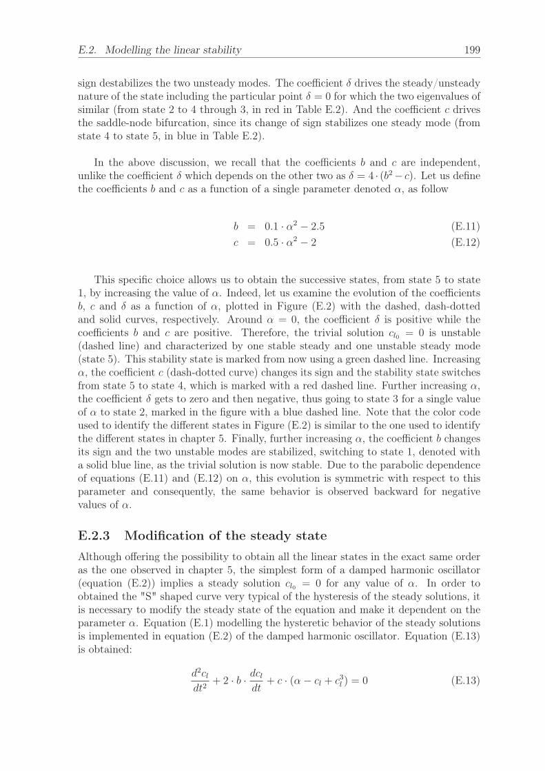
E.2. Modelling the linear stability 199
sign destabilizes the two unsteady modes. The coefficient δ drives the steady/unsteadynature of the state including the particular point δ = 0 for which the two eigenvalues ofsimilar (from state 2 to 4 through 3, in red in Table E.2). And the coefficient c drivesthe saddle-node bifurcation, since its change of sign stabilizes one steady mode (fromstate 4 to state 5, in blue in Table E.2).
In the above discussion, we recall that the coefficients b and c are independent,unlike the coefficient δ which depends on the other two as δ = 4 · (b2− c). Let us definethe coefficients b and c as a function of a single parameter denoted α, as follow
b = 0.1 · α2 − 2.5 (E.11)c = 0.5 · α2 − 2 (E.12)
This specific choice allows us to obtain the successive states, from state 5 to state1, by increasing the value of α. Indeed, let us examine the evolution of the coefficientsb, c and δ as a function of α, plotted in Figure (E.2) with the dashed, dash-dottedand solid curves, respectively. Around α = 0, the coefficient δ is positive while thecoefficients b and c are positive. Therefore, the trivial solution cl0 = 0 is unstable(dashed line) and characterized by one stable steady and one unstable steady mode(state 5). This stability state is marked from now using a green dashed line. Increasingα, the coefficient c (dash-dotted curve) changes its sign and the stability state switchesfrom state 5 to state 4, which is marked with a red dashed line. Further increasing α,the coefficient δ gets to zero and then negative, thus going to state 3 for a single valueof α to state 2, marked in the figure with a blue dashed line. Note that the color codeused to identify the different states in Figure (E.2) is similar to the one used to identifythe different states in chapter 5. Finally, further increasing α, the coefficient b changesits sign and the two unstable modes are stabilized, switching to state 1, denoted witha solid blue line, as the trivial solution is now stable. Due to the parabolic dependenceof equations (E.11) and (E.12) on α, this evolution is symmetric with respect to thisparameter and consequently, the same behavior is observed backward for negativevalues of α.
E.2.3 Modification of the steady state
Although offering the possibility to obtain all the linear states in the exact same orderas the one observed in chapter 5, the simplest form of a damped harmonic oscillator(equation (E.2)) implies a steady solution cl0 = 0 for any value of α. In order toobtained the "S" shaped curve very typical of the hysteresis of the steady solutions, itis necessary to modify the steady state of the equation and make it dependent on theparameter α. Equation (E.1) modelling the hysteretic behavior of the steady solutionsis implemented in equation (E.2) of the damped harmonic oscillator. Equation (E.13)is obtained:
d2cldt2
+ 2 · b · dcldt
+ c · (α− cl + c3l ) = 0 (E.13)

200 Appendix E. Design of the one-equation static stall model
−8 −6 −4 −2 0 2 4 6 8
α
−60
−40
−20
0
20
40
60
80Evolu
tion o
f para
mete
rs b
, c a
nd Δ
b
c
Δ
2 unsteady stable eigenvalues
2 unsteady unstable eigenvalues
2 unstable steady eigenvalues
1 stable and 1 unstable steady eigenvalues
Figure E.2: Representation of the steady state cl0 = 0 with the linearbehavior associated for each value of α (see associated color code inlegend). This linear behavior is based on the evolution of parameters b,c and δ also plotted. Every time that one of these parameters changesof sign, the linear behavior of the steady state evolves (as described inTable E.2. b is represented with a factor 8 and c with a factor 3 for
visualization purpose.
The linearization of the solution cl = cl0 + εc′l in equation (E.13) gives the twofollowing equations at orders ε0 and ε1.
ε0 : α− cl0 + c3l0 = 0
ε1 :d2c′ldt2
+ 2 · b · dc′l
dt+ c · (3 · c2l0 − 1) · c′l = 0
(E.14)
(E.15)
One can observe that the steady state (order ε0) is now dependent of the parameterα. From now, the computation of the steady state is less obvious than the previous caseand requires a numerical resolution as there is no exact solution. A pseudo arc-lengthmethod is developed with python for this simple one-equation model.
E.2.4 Modelling limit cycles
Equation (E.13) has the ability to replicate the shape of the steady states as well as theirlinear behavior with wisely chosen parameters. However, with such an equation, theunstable unsteady eigenvalues would generate unsteadiness that would grow to infinity.To avoid such a nonphysical behavior, it is necessary to add nonlinear saturation. Thecase of the Van der Pol oscillator is considered to ensure such a behavior. Equation(E.13) becomes :
d2cldt2
+ (2 · b+ c2l ) ·dcldt
+ c · (α− cl + c3l ) = 0 (E.16)

E.2. Modelling the linear stability 201
The linearization of the solution cl = cl0 + εc′l in equation (E.16) gives the twofollowing equations at order ε0 and ε1.
ε0 : α− cl0 + c3l0 = 0
ε1 :d2c′ldt2
+ (2 · b+ c2l0) ·dc′ldt
+ c · (3 · c2l0 − 1) · c′l = 0
(E.17)
(E.18)
By similarity with the case of a simple oscillator, the terms previously designatedas b, c and δ become B, C and Δ and are defined as following in equation (E.19):
⎧⎪⎨⎪⎩B = 2 · b+ c2l0C = c · (3 · c2l0 − 1)
Δ = (2 · b+ c2l0)2 − 4 · c · (3 · c2l0 − 1)
(E.19)
The main difference with the case of a simple oscillator is that, to ensure the correctlinear behavior of the steady solutions we previously had to define b and c as functionsof α. However, by adding the previously described nonlinearities, it appears that B, Cand Δ are now functions of the steady solution cl0 , which depends on α. Consequently,these parameters naturally evolve as functions of α, which simplifies the choice of pa-rameters b and c.
The equation of a damped harmonic oscillator (E.2) could be analytically resolved.However, the new form of the equation (E.16) requires a numerical resolution. Never-theless, it is possible to determine the expression of some particular points and have abetter understanding of the model. We recall that the Hopf bifurcations occurs whenB = 0. The corresponding values of the steady lift coefficients are cH±
l = ±√( − 2b),showing that the coefficient b should be negative to obtain the Hopf bifurcations of thesteady states in the model. They occur for the values α = cH±
l − (cH±l )3.
The saddle-node bifurcations arise when C = 0. The corresponding steady stateare thus defined by cSN±
c = ±√(1/3), showing that their value is independent of anyparameter. They occur for the angle of incidence α = cSN±
l − (cSN±l )3.
The transition from steady to unsteady states is obtained for Δ = 0. The valuesof the lift coefficient are then cD±
l = 2 · (b − 3 · c) ± 2 · √9 · c2 − 6 · b · c− c and areobtained for the angle of incidence αD± = cD±
l − cD±3l .
The existence of Hopf bifurcations and steady to unsteady transition in the modelconstrains the choice of the values of the parameters b and c as follows:
b < 0
9 · c2 − 6 · b · c− c > 0
(E.20)(E.21)
Morever, we would like to have Hopf bifurcations located on the upper or lowerbranches of the steady states, not on the middle branches. This additional constrainis written:

202 Appendix E. Design of the one-equation static stall model
cH+l > cSN+
l (E.22)
It leads to the following restriction in the choice of the coefficient b:
b < −1/6 (E.23)
Similarly, we would like to have C < 0 on the middle branch only. It means,c · (3 · c2l0 − 1) < 0. We already know that 3 · c2l0 − 1 is negative for cSN−
l < cl0 < cSN+l .
Precisely, the domain of existence of the middle branch is for cSN−l < cl0 < cSN+
l , so wewant the parameter C to have a sign evolution similar to the sign evolution of 3 ·c2l0 −1.The condition to ensure that is:
c > 0 (E.24)
Another requirement is to have the Hopf bifurcation on the upper branch appearingfor higher values of α than the Hopf bifurcation on the lower branch. This conditionsis satisfied if:
αH+ > αH− (E.25)
It yields to the following restriction in the choice of the coefficient b:
b > −1/2 (E.26)
To summarize, the parameters b and c are subject to the following restrictions inorder to replicate the linear behaviour wished:⎧⎪⎪⎨
⎪⎪⎩−1
6> b > −1
2
c > 0
(E.27)
One can also notice that with such ranges of existence, the condition 9·c2−6·b·c−c >0 is completely fulfilled.
Figure (E.3) shows the evolution of the steady states with the associated linearbehavior and the evolution of the parameters B, C and Δ (respectively dashed, dotted-dashed and full lines) in the particular case of b = −0.45 and c = 0.1 as an example.In this particular case, the parameters respect the aforementioned conditions: one cannote the appearance of the different linear state in the order detailed in subsection

E.2. Modelling the linear stability 203
E.2.1. By following the linear abscissa of the curve, one encounters first state 1 withtwo stable unsteady eigenvalues (full blue line), state 2 with two with two unstableunsteady eigenvalues (dashed blue line), state 3 with two unstable steady eigenvalues(dashed red line) and state 4 with one stable steady and one unstable steady eigen-values. The point (0,0) is a rotational symmetry centre of the curve and consequently,the same behavior is repeated on the other half of the curve.
−2.0 −1.5 −1.0 −0.5 0.0 0.5 1.0 1.5 2.0
α
−3
−2
−1
0
1
2
3
Evolu
tion o
f B
, C
and Δ
B
C
Δ
−1.5
−1.0
−0.5
0.0
0.5
1.0
1.5
cl 0
2 unsteady stable eigenvalues
2 unsteady unstable eigenvalues
2 unstable steady eigenvalues
1 stable and 1 unstable steady eigenvalues
Figure E.3: Representation of the steady state cl0 as a function of αwith the linear behavior associated for each value of α (see associatedcolor code in legend). This linear behavior is based on the evolutionof parameters B, C and Δ also plotted. Every time that one of theseparameters changes of sign, the linear behavior of the steady state evolves(as described in Table (E.2). Similar to Figure (E.2) but with non-nullsteady states and parameters B, C and Δ functions of the steady states.


205
Appendix F
Non-dominated Sorted GeneticAlgorithm
ContentsF.1 Introduction . . . . . . . . . . . . . . . . . . . . . . . . . . . 205
F.2 Steps and specific vocabulary . . . . . . . . . . . . . . . . . 206
F.2.1 Non-dominated sorting . . . . . . . . . . . . . . . . . . . . . . 206
F.2.2 Crowding distance . . . . . . . . . . . . . . . . . . . . . . . . 207
F.2.3 Parents selection . . . . . . . . . . . . . . . . . . . . . . . . . 207
F.2.4 Genetic modifications . . . . . . . . . . . . . . . . . . . . . . 207
F.2.5 Candidates for next generation . . . . . . . . . . . . . . . . . 208
F.2.6 Summary . . . . . . . . . . . . . . . . . . . . . . . . . . . . . 209
F.3 Application to a simple case . . . . . . . . . . . . . . . . . . 209
F.3.1 Selection for the next generation . . . . . . . . . . . . . . . . 209
F.3.2 Evolution of the Pareto front . . . . . . . . . . . . . . . . . . 210
The Non-dominated Sorting Genetic Algorithm II (NSGA-II) [37], is a genetic algo-rithm named after the method used to rank and select the solutions. NSGA-II uses thesame principle as NSGA but the computation time is reduced and a better diversity ofthe population is ensured in this version. This chapter is dedicated to the presentationof the algorithm : first, the different steps and the specific vocabulary are introduced,then a simple example is presented (also used to validate the code developed in python).
F.1 IntroductionThe principle of genetic algorithms is fundamentally different from the gradient basedmethods. Indeed, genetic algorithms are based on the evaluation of a large number ofsolutions to identify the best ones while gradient based methods consists in finding adescent direction to reach the best solution [153].

206 Appendix F. Non-dominated Sorted Genetic Algorithm
Genetics algorithms often refer to a very specific vocabulary, based on naturalselection:
- The term individuals refers to a solution to the considered problem. However,this is not necessarily a solution that minimizes the objective functions
- The term population refers to a set of individuals
- The term parents is used to characterized an individual which is considered togenerate new individuals
- The term offsprings is used to characterized the new individuals generated fromthe parents
- The term generation refers to the number of time the offsprings have been gen-erated. It can be seen as an iteration.
The approach of genetic algorithms is the following. A large population of randomlyset individuals is used to evaluate the two (or more) objective functions. First, a partof the population is selected to become parents. These parents generate offsprings bygenetic modification (crossover [36] or mutation). More practically, this means thatsome parents are mixed with others to create offsprings (crossover) while other parentsare slightly modified to generate other offsprings (mutation). Then, the initial popu-lation and the offsprings are evaluated and ranked based on the value of the objectivefunctions. The best solutions based on this ranking are used to become the next gen-eration. The process is repeated with this new population until convergence. In theend, a Pareto front of solutions is obtained: it offers a large population of solutionsthat fits more or less each objective function.
Let us consider a case with two objective functions Obj1 and Obj2 as an example.The Pareto front would be made of a solution that is an excellent fit for Obj1 buta poor fit for Obj2, of another solution that is, on the contrary, an excellent fit forObj2 and a poor fit for Obj1 and, in between, a large choice of solutions that arecompromises between these two extrema. This kind of algorithm is named after theparticular way to consider the problem as the evolution of a species that would natu-rally select the individuals which are the most adapted for certain conditions and hasthe advantage of offering several solutions that can be chosen.
F.2 Steps and specific vocabulary
F.2.1 Non-dominated sorting
This is the method used to rank the solutions. Let us consider the objective functionvector Obj(p), which gives the value of each objective function associated to the solu-tion p. A solution p is dominated by q if for each component i of the the vector Obj,Obj(p)i < Obj(q)i is never true and for at least one component Obj(p)i > Obj(q)i.The point of the method, is to evaluate the whole population and determine the non-dominated solutions which means that dominated by no other solutions. They are

F.2. Steps and specific vocabulary 207
gathered into the front number one and removed from the population. The sameprocess is repeated and this time the non-dominated solutions are gathered into thefront number two and so one until the whole population is ranked in fronts. A solu-tion is not necessary dominated or non-dominated by another solution but can alsobe neutral compared to another solution. For example, if we consider the objectivevectors associated to three solutions a, b and c : Obj(a) = (2, 1), Obj(b) = (1, 2) andObj(c) = (2, 2). a and b dominates c and so c is dominated by a and b. However, adoes not dominate b and neither the invert. Consequently, a and b are ranked in thefirst front and c in the second front.
Note that this method of evaluation, used in the original version of NSGA [153], canbe quite long as we have to compare each solution to all the others and do it until theyare all ranked. The updated version NSGA-II [37] actually performs the comparisononly once and, for each solution i, the number of other solutions that dominate i arestored as well as the indices of the solutions that are dominated by i. Consequently,by only performing the comparison once, all the data needed to rank the solutions arestored.
F.2.2 Crowding distance
This criteria is used to compare the solutions from a same front to ensure the diversityof the population. Indeed, it is preferable that the population does not converge toa particular solution but covers the whole field of possible solutions. To do so, thecrowding distance, which evaluates the distance to other solutions, is developed andused to ensure that between two solutions from the same front, the one with the largestcrowding distance is selected first (i.e. the solution the furthest from other solutions).This is a new feature of the NSGA-II as in the previous version, a user parameter wasused to maintain diversity of solutions which was more complex and less efficient.
F.2.3 Parents selection
The parents are selected using a tournament method: two individuals are randomlyselected from the population and compared. The best one is chosen to become a par-ent and removed from the population. The other one stays in the population. Theselection is made, first by comparing the front of the two individuals : the one in thelowest front is the best. If they are from the same front, their crowding distance iscompared : the one with the largest crowding distance is the best. With this method,half of the population is selected to become parents.
F.2.4 Genetic modifications
The point of this step is to create new solutions from the parents selected until the sizeof population has doubled. The offsprings are created by means of Simulated BinaryCrossover (SBX) and polynomial mutation with 90% chance of performing a SBX and10% of performing a mutation.

208 Appendix F. Non-dominated Sorted Genetic Algorithm
F.2.4.1 Crossover
Each crossover actually generates two children from two parents. The kth element ofeach offspring is defined as in equation (F.2):
Child1k =1
2[(1− βk) · Par1k + (1 + βk) · Par2k] (F.1)
Child2k =1
2[(1 + βk) · Par1k + (1− βk) · Par2k] (F.2)
where βk is a distribution obtained by generating a random number u for each compo-nent k in the law presented in equations (F.3) and (F.4). μc is a parameter that allowthe user to define how different the children is from the parents. In our case, we setμc = 5.
u ≤ 0.5 , βk(u) = (2 · u) 1μc+1 (F.3)
u > 0.5 , βk(u) =1
[2 · (1− u)]1
μc+1
(F.4)
F.2.4.2 Mutation
The mutation generates only one child from one parent by modifying the parent usingthe law presented on equation (F.5):
Childk = Park + δk (F.5)
with δk a distribution obtained by generating a random number u for each componentk in the law presented in equation (F.7). μm is a parameter that allow the user todefine how different the child is from the parent. In our case, we set μm = 10.
u < 0.5 , βk(u) = (2 · u) 1μm+1 − 1 (F.6)
u ≥ 0.5 , βk(u) = 1− [2 · (1− u)]1
μm+1 (F.7)
F.2.5 Candidates for next generation
The new population of size N made of initial population and the offsprings generated isranked and only the best half is kept for next generation. The non-dominated sortingcoupled with the crowding distance criteria is used. However, to avoid useless compu-tations, the population for next generation is selected as following. Let us designate by
nj the number of individuals of the jth front. K is the first front for whichK∑j=1
nj >N2.
All the individuals of the K−1 fronts are kept for next generation. For the elements ofthe Kth front a ranking based on the crowding distance is necessary : the individualsof the Kth front with the largest crowding distance are selected until N
2individuals
are selected. With such an approach the crowding distance is evaluated only for theindividuals in the front that has to be split.

F.3. Application to a simple case 209
F.2.6 Summary
All the steps described are summarized in the schema presented in Figure (F.1) (adaptedfrom [37]).
Initial
population
of size
N
Parents
Initial
population
of size
N
Offsprings
Front 1
Front 2
Front 3
Front 4
Front 5
Tournament
selection
Genetic
modifications
Non-
dominated
sorting
Front 4
sorted
Crowding
distance
sorting
Population
for next
generation
of size
N
Selected
for next
generation
Selected
for next
generation
Rejected
Rejected
Figure F.1: Schema of the various steps of the NSGA-II during ageneration. Adapted from [37]
F.3 Application to a simple caseWe want to find the best solutions (x, y) minimizing these two functions f and g.
f = (x− 1)2 + (y − 1)2 (F.8)g = (x+ 1)2 + (y + 1)2 (F.9)
The analytical solutions of this minimization problem are:
S = {(x, y) ∈ [−1, 1]× [−1, 1] | x = y} (F.10)
F.3.1 Selection for the next generation
Figure (F.2) presents the different steps of the selection process of the population thatis conserved from generation n to generation n+ 1.
The results of the tournament selection are depicted in Figure (F.2)(a). The initialpopulation is represented by black circles in the plane (f(x, y), g(x, y)). The individualswith a white cross are selected as parents. Note that with the tournament method, notonly the best individuals are selected. This method, although presenting the drawbackof missing a few good individuals, offers the advantage of preserving the diversity ofthe population as two "bad" parents not necessarily generate a "bad" offspring. Thechildren generated by the selected parents are presented in Figure (F.2)(b) by whitecircles. Finally, in Figure (F.2)(c), the individuals of the population chosen for nextgeneration are highlighted in red. Visually this corresponds to the individuals the moston the bottom/left part of the curve, which minimizes both objective functions.

210 Appendix F. Non-dominated Sorted Genetic Algorithm
(a) (b) (c)
Figure F.2: Evolution of the population at the different stages of ageneration. (a) Selection of parents. (b) Creation of offsprings. (c)
Selection of best parents and offsprings for the next generation.
F.3.2 Evolution of the Pareto front
This selection process is repeated during 50 generations and the results are presentedin Figure (F.3), which exhibits the population for different generations in red circlesand the theoretical Pareto front by a black line. One can observe how the populationget closer and closer to the Pareto front as the number of generations is increasing andhow the population is well spread on this front at the last generation.
One shall note that randomness is a big part of genetic algorithm (initial population,parents selection and genetic modifications). Consequently, running two times the sameoptimization problem might lead to two different ways to reach the Pareto front andthe number of generations needed for convergence might be different.

F.3. Application to a simple case 211
0 2000 4000 60000
2000
4000
6000
g(x
,y)
Generation n°0
Population Analytical Pareto front
0 500 10000
500
1000 Generation n°2
0 50 1000
50
100Generation n°4
0 20 400
10
20
30
g(x
,y)
Generation n°7
0 5 10 150.0
2.5
5.0
7.5 Generation n°10
0 5 10 150.0
2.5
5.0
7.5 Generation n°12
0 5 10
f(x, y)
0.0
2.5
5.0
7.5
g(x
,y)
Generation n°20
0.0 2.5 5.0 7.5
f(x, y)
0.0
2.5
5.0
7.5Generation n°35
0.0 2.5 5.0 7.5
f(x, y)
0.0
2.5
5.0
7.5 Generation n°50
Figure F.3: Visualization of the population (red circles) in the(f(x, y), g(x, y)) plane for several generations. Each circle correspondsto a couple (x, y). The theoretical Pareto front is represented by a black
line.


213
Bibliography
[1] S. Abhyankar, J. Brown, E. Constantinescu, D. Ghosh, B. F. Smith, andH. Zhang. PETSc/TS: A Modern Scalable ODE/DAE Solver Library. arXivpreprint arXiv:1806.01437, 2018.
[2] J. Almutairi and I. Alqadi. Large-eddy simulation of natural low-frequency os-cillations of separating-reattaching flow near stall conditions. AIAA Journal,51(4):981–991, 2013.
[3] J. Almutairi, I. Alqadi, and E. M. ElJack. Large eddy simulation of a NACA-0012airfoil near stall. Direct and Large-Eddy Simulation IX, 20, 2015.
[4] H.B. An, J. Wen, and T. Feng. On finite difference approximation of a matrix-vector product in the Jacobian-free Newton-Krylov method. Journal of Compu-tational an Applied Mathematics, 236:1399–1409, 2011.
[5] P. J. Ansell and M. B. Bragg. Characterization of ice-induced low-frequencyflowfield oscillations and their effect on airfoil performance. AIAA Journal, 2673,2013.
[6] P. J. Ansell and M. B. Bragg. Characterization of low-frequency oscillations inthe flowfield about an iced airfoil. AIAA Journal, 53(3):629–637, 2015.
[7] P. J. Ansell and M. B. Bragg. Unsteady modes in flowfield about airfoil withhorn-ice shape. Journal of Aircraft, 53(2), 2016.
[8] S. Bagheri, P. Schlatter, P. J. Schmid, and D. S. Henningson. Global stability ofa jet in crossflow. Journal of Fluid Mechanics, 624(33–44), 2009.
[9] B. S. Baldwin and T. J. Barth. A one-equation turbulence transport modelfor high Reynolds number wall bounded flows. NASA Technical Memorandum,102847, 1990.
[10] D. Barkley. Linear analysis of the cylinder wake mean flow. Europhysics Letter,75(5):750–756, 2006.
[11] D. Barkley, L. S. Tuckerman, and M. Golubitsky. Bifurcation theory for three-dimensional flow in the wake of a circular cylinder. The American PhysicalSociety, 61(5):5247–5252, 2000.
[12] G. K. Batchelor and A. E. Gill. Analysis of the stability of axisymmetric jets.Journal of Fluid Mechanics, 14(4):529–551, 1962.
[13] S. Beneddine. Global stability analysis of underexpanded screeching jets. Euro-pean Journal of Mechancs B/Fluids, 49:392–399, 2014.

214 BIBLIOGRAPHY
[14] S. Beneddine. Characterization of unsteady flow behavior by linear stability anal-ysis. PhD thesis, Ecole Polytechnique, 2017.
[15] S. Beneddine, D. Sipp, A. Arnault, J. Dandois, and L. Lesshafft. Conditions forvalidity of mean flow stability analysis. Journal of Fluid Mechanics, 798:485–504,2016.
[16] L. Bernardos, F. Richez, V. Gleize, and G. A. Gerolymos. Algebraic nonlocaltransition modeling of laminar separation bubbles using k−ω turbulence models.AIAA Journal, 57(2), 2019.
[17] N. Bonne. Stabilité de l’interaction onde de choc/couche limite laminaire. PhDthesis, Université Paris-Saclay - Ecole Polytechnique, 2018.
[18] J. L. Bonnet and C. Gleyzes. Etude expérimentale de la transition dans desbulbes de décollement laminaire au bord d’attaque des profils d’aile. RapportTechnique OA, 23(5018), 1983.
[19] M. B. Bragg, D. C. Heinrich, F. A. Balow, and K. B. M. Q. Zaman. Flowoscillation over an airfoil near stall. AIAA Journal, 34(1):199–201, 1996.
[20] M. B. Bragg and K. B. M. Q. Zaman. Flow oscillation over airfoils near stall.International Council of the Aeronautical Sciences, 4(5):1639–1648, 1994.
[21] J. Brewster and M. P. Juniper. Shape sensitivity of eigenvalues in hydrodynamicstability, with physical interpretation for the flow around a cylinder. EuropeanJournal of Mechancs B/Fluids, 80:80–91, 2019.
[22] A. P. Broeren. Phase-averaged LDV flowfield measurements about an airfoil inunsteady stall. AIAA Journal, 2494:921–931, 1996.
[23] A. P. Broeren and M. B. Bragg. Flowfield measurements over and airfoil duringnatural low-frequency oscillations near stall. AIAA Journal, 37(1):130–132, 1998.
[24] A. P. Broeren and M. B. Bragg. Low frequency flowfield unsteadiness duringairfoil stall and the influence of stall type. AIAA Paper, 2517(196–209), 1998.
[25] A. P. Broeren and M. B. Bragg. Spanwise variation in the unsteady stallingflowfields of two-dimensional airfoil models. AIAA Journal, 37(1):130–132, 2001.
[26] A. P. Broeren, B. S. Woodard, J. M. Diebold, and F. Moens. Low-Reynoldsnumber aerodynamics of an 8.9 percent scale semispan swept wing for assessmentof icing effects. NASA Technical Memorandum, 219533, 2017.
[27] L. Cambier, M. Gazaix, S. Heib, S. Plot, M. Poinot, J.-P. Veuillot, J.-F. Bous-suge, and M. Montagnac. An Overview of the Multi-Purpose elsA Flow Solver.AerospaceLab, pages 1–15, 2011.
[28] P. Chassaing. Turbulence en mecanique des fluides. Cepadues-Editions, 2000.
[29] J.-M. Chomaz. Global instabilities in spatially developping flows: non-normalityand nonlinearity. Annual Review of Fluid Mechanics, 37:357–392, 2005.

BIBLIOGRAPHY 215
[30] C. Cossu, G. Pujals, and S. Depardon. Optimal transient growth and verylarge-scale structures in turbulent boundary layers. Journal of Fluid Mechan-ics, 619:79–94, 2009.
[31] D. Crighton and M. Gaster. Stability of slowly diverging jet flow. Journal ofFluid Mechanics, 77(2):397–413, 1976.
[32] J. D. Crouch, A. Garbaruk, and D. Magidov. Predicting the onset of flowunsteadiness based on global instability. Journal of Computational Physics,224:924–940, 2007.
[33] J. D. Crouch, A. Garbaruk, D. Magidov, and A. Travin. Origin of transonicbuffer on aerofoils. Journal of Fluid Mechanics, 628:357–369, 2009.
[34] T. Cui, W. Liao, and D. Yu. Topological approach for analyzing and modelingthe aerodynamic hysteresis of an airfoil. Computer Modeling in Engineering andSciences, 45(3):273–293, 2009.
[35] G. de Vries. Multiple bifurcations in a polynomial model of bursting oscillations.Journal of Nonlinear Sciences, 8:281–316, 1998.
[36] K. Deb and R. B. Agarwal. Simulated Binary Crossover for Continuous SearchSpace. Complex Systems, 9:115–148, 1995.
[37] K. Deb, A. Pratap, S. Agarwal, and T. Meyarivan. A Fast and Elitist Multi-objective Genetic Algorithm: NSGA-II. IEEE Transactions on EvolutionnaryComputation, 6(2), 2002.
[38] S. Deck. Simulation numérique des charges latérales instationnaires sur des con-figurations de lanceur. PhD thesis, Université d’Orléans, 2002.
[39] A. Dhooge, W. Govaerts, Y. A. Kuznetsov, H. G. E. Meijer, and B. Sautois. Newfeatures of the software MatCont for bifurcation analysis of dynamical systems.Mathematical and Computer Modelling of Dynamical Systems, 14(2):147–175,2008.
[40] K. I. Dickson, C. T. Kelley, I. C. F. Ipsen, and I. G. Kevrekidis. Condition esti-mates for pseudo-arclength continuation. SIAM Journal on Numerical Analysis,45(1):263–276, 2006.
[41] H. A. Dijkstra, F. W. Wubs, A. K. Cliffe, E. Doedel, I. F. Dragomirescu, B. Eck-hardt, A. Y. Gelfgat, A. L. Hazel, V. Lucarini, A. G. Salinger, E. T. Phipps,J. Sanchez-Umbria, H. Schuttelaars, L. S. Tuckerman, and U. Thiele. Numericalbifurcation methods and their application to fluid dynamics: analyysis beyondsimulation. Communication on Computational Physics, 15(1):1–45, 2014.
[42] G. Dimitriadis and J. Li. Bifurcation behavior of airfoil undergoing stall flutteroscillations in low-speed wind tunnel. AIAA Journal, 47(11):2577–2596, 2009.
[43] S. Diwan, S. Chetan, and O. Ramesh. On the bursting criterion for laminarseparation bubbles. IUTAM Symposium on Laminar-Turbulent Transition, pages401–407, 2006.

216 BIBLIOGRAPHY
[44] A. V. Dovgal. Development of vortical disturbances in flow with laminar sep-aration. Laminar-Turbulent Transition, Proceedings of the IUTAM-Symposium,pages 359–366, 1985.
[45] P. G. Drazin. On a model of instability of a slowly-varying flow. The QuarterlyJournal of Mechanics and Applied Mathematics, 27(1):69–86, 1974.
[46] J. R. Edwards and S. Chandra. Comparison of eddy viscosity-transport turbu-lence models for three-dimensional, shock-separated flowfields. AIAA Journal,34(4):756–763, 1996.
[47] J. R. Edwards and M.-S. Liou. Low-diffusion flux splitting methods for flows atall speeds. AIAA Journal, 36:1610–1617, 1998.
[48] J. A. Ekaterinaris and F. R. Menter. Computation of oscillating airfoil flowswith one- and two-equation turbulence models. AIAA Journal, 32(12):2359–2365, 1994.
[49] E. M. ElJack and J. Soria. Bursting and reformation cycle of the laminar sep-aration bubble over a NACA-0012 aerofoil: the underlying mechanism. arXiv,2018.
[50] H. A. Eschenauer. Multicriteria optimization for highly accurate focusing sys-tems. Multicritera Optimization in Engineering and Sciences - MathematicalConcepts and Methods in Science and Engineering, 37(309-354), 1988.
[51] D. Fabre, F. Auguste, and J. Magnaudet. Bifurcations and symmetry breakingin the wake of axisymmetric bodies. Physics of Fluids, 20(051702):1–4, 2008.
[52] H. Fallah. Symmetric fold/super-Hopf bursting, chaos and mixed-mode oscil-lations in Pernarowski model of pancreatic beta-cells. International Journal ofBifurcation and Chaos, 26(09), 2016.
[53] A. Favre. Equations des gaz turbulents compressibles, part 1: formes générales.Journal de Mécanique, 4:361–390, 1965.
[54] A. Favre. Equations des gaz turbulents compressibles, part 2: méthode desvitesses moyennes; méthode des vitesses moyennes pondérées par la masse volu-mique. Journal de Mécanique, 4:391–421, 1965.
[55] A. D. Gardner, K. Richter, and H. Rosemann. Nuerical investigation of air jets fordynamic stall control on the OA209 airfoil. CEAS Aeronautical Journal, 1:69–82,2011.
[56] M. Gaster. The structure and behaviour of separation bubbles. A.R.C. Reportsand Memoranda, 3595, 1967.
[57] T. B. Gatski and J.-P. Bonnet. Compressibility, turbulence and high speed flow.Elsevier, 2009.
[58] D. E. Gault. A correlation of low-speed, airfoil-section stalling characteristicswith Reynolds number and airfoil geometry. NACA Technical Note, 3963, 1957.

BIBLIOGRAPHY 217
[59] F. Giannetti and P. Luchini. Structural sensitivity of the first instability of thecylinder wake. Journal of Fluid Mechanics, 581:167–197, 2007.
[60] R. Gilmore. Catastrophe theory for scientists and engineers. Dover Publications,1993.
[61] V. Gleize, J. Szydlowski, and M. Costes. Numerical and physical analysis ofturbulent viscous flow around a NACA0015 profile at stall. European Congresson Computational Methods in Applied Sciences and Engineering, 2004.
[62] C. Gleyzes, C. Cousteix, and J. L. Bonnet. Theoretical and experimental studyof low Reynolds-number transitional separation bubbles. In Conference on LowReynolds Number Airfoil Aerodynamics, Notre Dame, IN, 137-152, 1985.
[63] W. Govaerts. Numérical methods for bifurcations of dynamical equilibria. Siam,2000.
[64] A. Harten and J. M. Hyman. Self adjusting grid methods for one-dimensionalhyperbolic conservation laws. Journal of Computational Physics, 50(2):235–269,1983.
[65] A. Hatman and T. Wang. Separated-Flow transition. PART 1 - Experimentalmethodology and mode classification. PART 2 - Experimental results. PART 3 -Primary modes and vortex dynamics. ASME Paper, 98(461–462–463), 1998.
[66] D. C. Hill. A theoretical approach for analyzing the restabilization of wakes.NASA Technical Memorandum, 103858, 1992.
[67] J. A. Hoffman. Effects of freestream turbulence on the performance characteris-tics of an airfoil. AIAA Journal, 29(9):1353–1354, 1991.
[68] H. P. Horton. Laminar separation bubbles in two and three dimensional incom-pressible flow. PhD thesis, University of London - Queen Mary College - Depart-ment of Aeronautical Engineering, 1968.
[69] G. Hristov. Post-stall hysteresis and flow field unsteadiness on a NACA0012airfoil. PhD thesis, University of Illinois ar Urbana-Champaign, 2017.
[70] G. Hristov and P. J. Ansell. Post-stall hysteresis and flow field unsteadinesson a NACA0012 airfoil. AIAA SciTech Forum, 55th AIAA Aerospace SciencesMeeting, 2017.
[71] H. Hu, Z. Yang, and H. Igarashi. Aerodynamic hysteresis of a low-Reynolds-number airfoil. Journal of Aircraft, 44(6):2083–2086, 2007.
[72] P. Huerre and P. A. Monkewitz. Absolute and convective instabilities in freeshear layers. Journal of Fluid Mechanics, 159(151–168), 1985.
[73] P. Huerre and P. A. Monkewitz. Local and global instabilities in spatially devel-oping flows. Annual Review of Fluid Mechanics, 22:473–357, 1990.
[74] M. Illsley. https://bigsynthesis.com/understandingaerospace/index.php/6-why-are-helicopters-so-slow/. Website, 2014.

218 BIBLIOGRAPHY
[75] M. C. Iorio, L. M. Gonzalez, and E. Ferrer. Direct and adjoint global stabilityanalysis of turbulent transonic flows over a NACA0012 profile. InternationalJournal for Numerical Methods in Fluids, 76:147–168, 2014.
[76] M. C. Iorio, L. M. Gonzalez, and A. Martinez-Cava. Global stability analysis ofa compressible turbulent flow around a high-lift configuration. AIAA Journal,54(2):373–385, 2015.
[77] Richard P. Dwight Jacques E. V. Peter. Numerical sensitivity analysis for aerody-namic optimization: a survey of approaches. Computers and Fluids, 39:373–391,2010.
[78] R. Jain, A. Le Pape, A. Grubb, M. Costes, F. Richez, and M. Smith. High-resolution computational fluid dynamics predictions for the static and dynamicstall of a finite-span OA209 wing. Journal of Fluids and Structures, 78:126–145,2018.
[79] B. M. Jones. An experimental study of the stalling of wings. R. & M., 1588,1933.
[80] B. M. Jones. Stalling. Journal of the Royal Aeronautical Society, 38(285):753–770, 1934.
[81] W. P. Jones and B. E. Launder. The calculation of low-Reynolds-number phe-nomena with a two-equation model of turbulence. Journal Heat Mass, 16:1119–1130, 1973.
[82] M. P. Juniper and B. Pier. The structural sensitivity of open shear flows cal-culated with a local stability analysis. European Journal of Mechancs B/Fluids,49:426–437, 2015.
[83] T. Von Kármán. Ueber den Mechanismus des Widerstandes, den ein bewegterKörper in einer Flüssigkeit erfährt. Nachrichten von der Gesellschaft der Wis-senschaften zu Göttingen, Mathematisch-Physikalische Klasse, pages 509–511,1911.
[84] T. Von Kármán. Ueber den Mechanismus des Widerstandes, den ein bewegterKörper in einer Flüssigkeit erfährt. Nachrichten von der Gesellschaft der Wis-senschaften zu Göttingen, Mathematisch-Physikalische Klasse, pages 547–556,1912.
[85] K. Kaufman, M. Costes, F. Richez, A. D. Gardner, and A. Le Pape. Numeri-cal investigation of three-dimensional static and dynamic stall on a finite wing.Journal of the American Helicopter Society, 60, 2015.
[86] H. B. Keller. Lectures on numerical methods in bifurcation problems. H. Goctzc,Springer-Verlag, 1986.
[87] C. T. Kelley. Solving nonlinear equations with Newton’s method. Society forIndustrial and Applied Mathematics, 2003.

BIBLIOGRAPHY 219
[88] D.A. Knoll and D.E. KEYES. Jacobian-free Newton-Krylov methods: a surveyof approaches and applications. Journal of Computational Physics, 193:357–397,2004.
[89] Y. A. Kuznetsov. Elements of applied bifurcation theory, second edition. Springer,2004.
[90] B. Van Leer. Towards the ultimate conservative difference scheme. II. Mono-tonicity and conservation combined in a second-order scheme. Journal of Com-putational Physics, 14(4):361–370, 1974.
[91] P. Luchini, F. Giannetti, and J. Pralits. Structural sensitivity of linear andnonlinear global modes. AIAA Paper, 4227, 2008.
[92] C. K. Mamun and L. S. Tuckerman. Asymmetry and Hopf bifurcation in sphericalCouette flow. Physics of Fluids, 7:80–91, 1995.
[93] J. F. Marchman, Y. K. Chang, and R. D. Robinson. Sweep effects on lowReynolds number stall hysteresis. AIAA Paper, 88(4419), 1988.
[94] J. F. Marchman, V. Sumantran, and C. G. Schaefer. Acoustic and turbulenceinfluences on stall hysteresis. AIAA Journal, 25(1):50–51, 1987.
[95] O. Marquet and L. Lesshafft. Identifying the acive flow regions that drive linearand nonlinear instabilities. arXiv.
[96] O. Marquet, M. Lombardi, D. Sipp, J. M. Chomaz, and L. Jacquin. Direct andadjoint global modes of recirculation bubble: lift-up and convectire nonnormali-ties. Journal of Fluid Mechanics, 622(1–21), 2009.
[97] O. Marquet, D. Sipp, and L. Jacquin. Sensitivity analysis and passive control ofcylinder flow. Journal of Fluid Mechanics, 615:221–252, 2008.
[98] I. Mary. Méthode de newton approchee pour le calcul d’écoulements instation-naires comportant des zones à très faibles nombres de Mach. PhD thesis, Uni-versité Paris XI, 1999.
[99] I. Mary and P. Sagaut. Large eddy simulation of flow around an airfoil near stall.AIAA Journal, 40(6):1139–1145, 2002.
[100] W. J. McCroskey. Unsteady airfoil. Annual Review of Fluid Mechanics, 14:285–311, 1982.
[101] W. J. McCroskey and R. K. Fisher. Dynamic stall of airfoils and helicopterrotors. AGARD R, 595:2.1–2.7, 1972.
[102] G. B. McCullough and D. E. Gault. Examples of three representative types ofairfoil section sall at low speed. NACA Technical Note, 2502, 1951.
[103] H. G. E. Meijer. Matcont Tutorial: ODE GUI version. 2014.
[104] H. G. E. Meijer. Matcont Tutorial: ODE GUI version. 2016.

220 BIBLIOGRAPHY
[105] P. Meliga, J.-M. Chomaz, and D. Sipp. Global mode interaction and patternselection in the wake of a disk: a weakly nonlinear expansion. Journal of FluidMechanics, 633:159–189, 2009.
[106] P. Meliga, J.-M. Chomaz, and D. Sipp. Unsteadiness in the wake of disks andspheres: instability, receptivity and control using direct and adjoint global sta-bility analyses. Journal of Fluids and Structures, 25:601–616, 2009.
[107] F. R. Menter. Zonal two equation k−ω turbulence models for aerodynamic flows.AIAA Paper, 93-2906, 1993.
[108] C. Mettot, F. Renac, and D. Sipp. Computation of eigenvalue sensitivity to baseflow modification in a discrete framework: Application to open-loop control.Journal of Computational Physics, 269:234–258, 2014.
[109] C. B. Millikan and A. L. Klein. The effect of turbulence. Aircraft Engineering,5(8):169–174, 1933.
[110] S. Mittal and P. Saxena. Hysteresis in flow past a NACA 0012 airfoil. Computermethods in applied mechanics and engineering, 191:2179–2189, 2001.
[111] M. Mizoguchi, Y. Kajikawa, and H. Itoh. Static stall hysteresis of low-aspect-ratiowings. 32nd AIAA Applied Aerodynamic Conference, 2014.
[112] M. V. Morkovin. Effects of compressibility on turbulent flows. A. Favre (e),Mécanique de la turbulence, pages 367–380, 1962.
[113] T. J. Mueller. The influence of laminar separation and transition on low Reynoldsnumber airfoil hysteresis. Journal of Aircraft, 22(9):763–770, 1985.
[114] T. J. Mueller, L. J. Pohlen, P. E. Conigliaro, and B. J. Jansen. The influenceof free-stream disturbances on low Reynolds number airfoil experiments. Exper-iments in Fluids, 1:3–14, 1983.
[115] M. Nagata. Three-dimensional traveling-wave solutions in plane Couette flow.Physical Review E, 55(2):2023–2025, 1997.
[116] T. Nakazawa and H. Azegami. Shape optimization of flow field improving hy-drodynamic stability. Japan Journal of Industrial and Applied Mathematics,33:167–181, 2016.
[117] I. Newton. The Mathematical Papers of Isaac Newton, volume 2. CambridgeUniversity Press, 1968.
[118] M. M. O’meara and T. J. Mueller. Experimental determination of the lami-nar separation bubble characteristics of an airfoil at low Reynolds numbers. InAIAA/ASME 4th Fluid Mechanics, Plasma Dynamics and Lasers Conference,Atlanta, USA, 1986.
[119] P. R. Owen and L. Klanfer. On the laminar boundary layer separation from theleading edge of a thin airfoil. A.R.C. Technical Report, 220, 1955.

BIBLIOGRAPHY 221
[120] J.-Y. L’Excellent P. Amestoy, I. Duff and J. Koster. A fully asynchronous mul-tifrontal solver using distributed dynamic scheduling. SIAM Journal on MatrixAnalysis and Applications, 23(1):15–41, 2001.
[121] G. Pailhas, R. Houdeville, P.Barricau, A. Le Pape, A. Faubert, P. Loiret, andF. David. Experimental investigation of dynamic stall. 31th European RotorcraftForum, Florance, Italy, 2005.
[122] E. Paladini. Insight on transonic buffet instability - Evolution from two dimen-sional aerofoils to three-dimensional swept wings. PhD thesis, Ecole NationaleSuperieure d’Arts et Metiers - ENSAM, 2019.
[123] E. Paladini, O. Marquet, D. Sipp, J.-C. Robinet, and J. Dandois. Various ap-proaches to determine active regions in an unstable global mode: application totransonic buffet. Journal of Fluid Mechanics, 881:617–647, 2019.
[124] A. Le Pape, C. Lienard, and J. Bailly. Active flow control for helicopters.AerospaceLab Journal, 6, 2013.
[125] A. Le Pape, G. Pailhas, F. David, and J. M. Deluc. Extensive wind tunnelmeasurements of dynamic stall phenomenon for the OA209 airfoil including 3Deffects. In 33rd European Rotocraft Forum, Kazan, Russia, 2007.
[126] M. Pernarowski. Fast subsystem bifurcations in a slowly varying Liénard systemexhibiting bursting. SIAM Journal of Applied Mathematics, 54:814–832, 1994.
[127] E. Piot, G. Casalis, F. Muller, and C. Bailly. Investigation of the PSE approachfor subsonic an supersonic hot jets. Detailed comparisons with LES and linearizedEuler equations results. Internal Journal of Aeroacoustics, 5(4), 2006.
[128] R. Piziali. 2D and 3D oscillating wing aerodynamics for a range of angles of attackincluding stall. NASA Technical Memorandum, 4632(USAATCOM TechnicalReport 94-A-011), 1994.
[129] L. J. Pohlen and T. J. Mueller. Boundary layer characteristics of the Miley airfoilat low Reynolds numbers. Journal of Aircraft, 21(9):658–664, 1984.
[130] D. C. Sorensen R. B. Lehoucq and C. Yang. ARPACK Users Guide : Solutionof Large Scale Eigenvalue Problems by Implicitly Restarted Arnoldi Methods.Philadelphia: SIAM, 1998.
[131] J. Raphson. Analysis aequationum universalis. Tho. Braddyll, 1697.
[132] O. Reynolds. On the dynamical theory of incompressible viscous fluids and thedermination of the criterion. Proceedings of the Royal Society of London, 56:40–45, 1895.
[133] F. Richez, M. Leguille, and O. Marquet. Selective Frequency Damping methodfor steady RANS solutions of turbulent separated flows around an airfoil at stall.Computers and Fluids, 132:51–61, 2016.

222 BIBLIOGRAPHY
[134] F. Richez, I. Mary, V. Gleize, and C. Basdevant. Zonal RANS/LES couplingsimulation of a transitional and separated flow around an airfoil near stall. The-oretical and Computational Fluid Dynamics, 22:305–315, 2008.
[135] F. Richez, A. Le Pape, and M. Costes. Zonal detached-eddy simulation of sepa-rated flow around a finite-span wing. AIAA Journal, 53(11):3157–3166, 2015.
[136] F. Richez, A. Le Pape, M. Costes, and R. Gavériaux. Zonal detached-eddysimulation (ZDES) of the three dimensional stalled flow around a finite spanwing. In 42nd AIAA Fluid Dynamics Conderence and Exhibit, New Orleans,Louisiana, 2012.
[137] K. Richter, A. Le Pape, T. Knopp, M. Costes, V. Gleize, and A. D. Gardner.Improved two-dimensional dynamic stall prediction with structured and hybridnumerical methods. Journal of the American Helicopter Society, 45, 2011.
[138] K. Rinoie and N. Takemura. Oscillating behaviour of laminar separation bubbleformed on an aerofoil near stall. Aeronautical Journal, 108(1081):153–163, 2004.
[139] D. Rodriguez, E. M. Gennaro, and M. P. Juniper. The two classes of primarymodal instability in laminar separation bubbles. Journal of Fluid Mechanics,734(4):1–11, 2013.
[140] I. Rodriguez, O. Lehmkuhl, R. Borrell, and A. Oliva. Direct numerical simulationof a NACA0012 in full stall. International Journal of Heat and Fluid Flow,43:194–203, 2013.
[141] P. L. Roe. Approximate Riemann solvers, parameter vectors and differenceschemes. Journal of Computational Physics, 43(2):357–372, 1981.
[142] A. Roshko. On the drag and shedding frequency of two dimensional bluff bodies.NACA Technical Note, 3169, 1954.
[143] Y. Saad. Numerical methods for large eigenvalue problems. Siam, 1992.
[144] L. Sankar, J. Zibi-Bailly, J. C. Le Balleur, D. Blaise, O. Rouzaud, and M. Rhee.A comparative study of three methodologies for modeling dynamic stall. In 28thEuropean Rotorcraft Forum, Bristol, UK, 2002.
[145] F. Sartor, C. Mettot, and D. Sipp. Stability, receptivity and sensitivity analysesof buffeting transonic flow over a profile. AIAA Journal, 53(7):1980–1993, 2015.
[146] F. W. Schmitz. Aerodynamics of the model airplane, Part I, Airfoil measure-ments. NASA Technical Memorandum, 60976, 1967.
[147] M. S. Selig, J. J. Guglielmo, A. P. Broeren, and P. Giguere. Experiments onairfoils at low Reynolds numbers. AIAA Paper, 0062, 1996.
[148] D. Sipp. Open-loop control of cavity oscillations with harmonic forcings. Journalof Fluid Mechanics, 708:439–468, 2012.

BIBLIOGRAPHY 223
[149] D. Sipp and A. Lebedev. Global stability of base and mean flows: a generalapproach and its applications to cylinder and open cavity flows. Journal of FluidMechanics, 593:333–358, 2007.
[150] D. Sipp, O. Marquet, P. Meliga, and A. Barbagallo. Dynamics and controlof global instabilities in open-flows: a linearized approach. Applied MechanicalReview, 63, 2010.
[151] P. R. Spalart and S. R. Allmaras. A one-equation turbulence model for aerody-namic flows. La recherche aérospatiale, 1:5–21, 1994.
[152] P. R. Spalart and C. L. Rumsey. Effective inflow conditions for turbulence modelsin aerodynamic calculations. AIAA Journal, 45(10):2544–2553, 2007.
[153] N. Srinivas and K. Deb. Multiobjective Optimization Using Nondominated Sort-ing in Genetic Algorithms. Evolutionnary Computations, 2(3):221–248, 1994.
[154] G. R. Srinivasan, J. A. Ekaterinaris, and W. J. McCroskey. Evaluation of turbu-lence models for unsteady flows of an oscillating airfoil. Computers and Fluids,24(7):833–861, 1995.
[155] S. H. Strogatz. Nonlinear dynamics and chaos: with applications to physics,biology, chemistry and engineering. Addison-Wesley Publishing Company, 1994.
[156] J. Szydlowski and M. Costes. Simulation of flow around a static and oscillat-ing pitching NACA0015 airfoil using URANS and DES. ASME Transfer/FluidsEngineering Summer Conference, 2004.
[157] H. Tanaka. Flow visualization and PIV measurements of laminar separation bub-ble oscillating at low frequency on an airfoil near stall. In International Councilof the Aeronautical Sciences Paper, editor, 24th Congress of International Coun-cil of the Aeronautical Sciences, 2004.
[158] I. Tani. Low-speed flows involving bubble separations. Progress in AerodynamicalSciences, 5:70–103, 1964.
[159] A. Tezuka and K. Suzuki. Three-dimensional global linear stability analysis offlow around a spheroid. AIAA Journal, 44:1697–1708, 2006.
[160] V. Theofilis. Advances in global linear instability of nonparallel and three-dimensional flows. Progress in Aerospace Sciences, 39(4):249–315, 2003.
[161] V. Theofilis. Global linear instability. Annual Review of Fluid Mechanics, 43:319–352, 2011.
[162] V. Theofilis, S. Hein, and U. Dallmann. On the origins of unsteadiness and three-dimensionality in a laminar separation bubble. Philosophical Transactions of theRoyal Society of London, 358, 2000.
[163] J. J. Thibert, M. Grandjacques, and L. H. Ohman. Experimental database forcomputer program assessment. AGARD Advisory Report, 138(A1), 1979.

224 BIBLIOGRAPHY
[164] E. Torenbeek. Synthesis of subsonic airplan design. Delft University Press, 1982.
[165] L. S. Tuckerman and D. Barkley. Bifurcation analysis for timesteppers. Numer-ical methods for bifurcation problems and large-scale dynamical systems. IMAVolumes in Mathematics and its Applications, 119:453–466, 2000.
[166] C. Wales, A. L. Gaitonde, D. P. Jones, D. Avitabile, and A. R. Champneys.Numerical continuation of high Reynolds number external flows. Internationaljournal for numerical methods in fluids, 68:135–159, 2012.
[167] J. H. Watmuff. Evolution of a wave packet into vortex loops in a laminar sepa-ration bubble. Journal of Fluid Mechanics, 119–169, 397.
[168] D. C. Wilcox. Reassessment of the scale-determining equation for advanced tur-bulence models. AIAA Journal, 26(11):1299–1310, 1988.
[169] Z. Yang, H. Igarashi, M. Martin, and H. Hu. An experimental investigation onaerodynamic hysteresis of a low-Reynolds number airfoil. AIAA Paper, 315, 2008.
[170] S. Yon and J. Katz. Study of the unsteady flow features on a stalled wing. AIAAJournal, 3(305–312), 36.
[171] S. Yoon and A. Jameson. An LU-SSOR scheme for the Euler and Navier-Stokesequations. NASA Contractor Report, 179556, 1986.
[172] K. B. M. Q. Zaman, A. Bar-Sever, and S. M. Mangalam. Effect of acousticexcitation over airfoils near stall. Journal of Fluid Mechanics, 182:127–148, 1987.
[173] K. B. M. Q. Zaman, D. J. McKinzie, and C. L. Rumsey. A natural low-frequencyoscillation of the flow over an airfoil near stalling conditions. Journal of FluidMechanics, 54:403–442, 1989.


Titre: Étude d’un écoulement turbulent à haut nombre de Reynolds autour d’un profil proche du décrochage; une approchecouplant formalisme RANS et théorie de la bifurcation
Mots clés: décrochage, stabilité globale, théory de la bifurcation, RANS, écoulement turbulent
Résumé: Le phénomène de décrochage est souvent décritcomme une chute soudaine de portance lorsque l’angled’incidence augmente, ce qui est préjudiciable aux avionset aux hélicoptères. Plusieurs études numériques et ex-périmentales ont révélé des phénomènes apparaissant prochede l’angle de décrochage : plusieurs angles d’attaque pourlesquels l’écoulement est bistable et des oscillations bassesfréquences à un nombre de Strouhal particulier de St ∼ 0.02.L’objectif de cette thèse est d’avoir une meilleure compréhen-sion de l’origine du décrochage et de ces deux phénomènesgrâce à des simulations numériques d’écoulements turbulentsmodélisés par une approche RANS. Une combinaison de di-verses approches numériques et théoriques (simulations insta-tionnaires, continuation de solutions stationnaires, stabilitélinéaire et analyse de bifurcation) est développée et appliquéedans le cas du décrochage d’un profil 2D de pale d’hélicoptère,le OA209, à bas nombre de Mach (M ∼ 0.2) et haut nombrede Reynolds (Re ∼ 1.8× 10⁶).Des solutions stationnaires sont calculées pour différents an-gles d’attaque en considérant le modèle de turbulence deSpalart-Allmaras et en utilisant des méthodes de continu-ation. Les résultats mettent en évidence la bistabilité de
l’écoulement pour plusieurs angles proches du décrochage.Des analyses de stabilité linéaire réalisées autour de ces étatsd’équilibres révèlent l’existence d’un mode instable bassefréquence associé au décrochage. L’évolution des valeurspropres associées à ce mode le long des branches station-naires nous permet d’établir une première version du dia-gramme de bifurcation. Afin de le compléter, des calculsRANS instationnaires sont réalisés et des cycles limites bassefréquence de large amplitude sont identifiés sur une plageréduite d’angles d’attaque proches du décrochage. Pour clar-ifier la formation et la disparition de ces cycles limites bassefréquence et permettre une meilleure compréhension du scé-nario de bifurcation, un modèle à une équation reproduisantles caractéristiques linéaires du phénomène est proposé. Cemodèle non-linéaire du décrochage statique est calibré sur lesétats stationnaires, et leur comportement linéaire, obtenuspar calculs RANS. Une étude du comportement non-linéairede ce modèle révèle un scenario possible qui pourrait con-duire à l’apparition et à la disparition de cycles limites bassefréquence. Finalement, le cas d’un NACA0012 à nombre deReynolds Re ∼ 1.0 × 10⁶ est considéré pour valider la ro-bustesse du scenario identifié.
Title: Study of a high Reynolds number flow around a two dimensional airfoil at stall; an approach coupling a RANSframework and bifurcation theory
Keywords: stall, global stability, bifurcation theory, RANS, turbulent flow
Abstract: Airfoil stall is commonly described as a suddendrop of lift when increasing the angle of attack, which is detri-mental to aircraft and helicopters. Past experimental andnumerical investigations have clearly identified two phenom-ena which can appear close to the stall angle: several anglesof attack for which the flow is bistable and low frequencyoscillations at the particular Strouhal number of St ∼ 0.02.The objective of this thesis is to better understand the originof stall and of these two phenomena using numerical simu-lations of turbulent flows modeled in the RANS framework.A combination of numerical and theoretical approaches (un-steady simulations, continuation of steady solutions, linearstability and bifurcation analyses) have been developed andapplied to the case of a 2D OA209 airfoil at low Mach number(M ∼ 0.2) and high Reynolds number (Re ∼ 1.8× 10⁶).Steady RANS computations are performed using the Spalart-Allmaras model to obtain steady states for several anglesof attack taking advantage of continuation methods. Theresults highlight the bistability of the flow for several an-gles of attack near stall. Linear stability analyses performed
around these equilibrium states reveal the existence of a low-frequency unstable mode associated with stall. The evolutionof the corresponding eigenvalues along the branches of steadysolutions allows us to establish a first sketch of the bifurca-tion scenario. Unsteady RANS computations are carried outto complete it. Large amplitude low-frequency limit-cyclesolutions are identified in a narrow range of angles of attackclose to stall. To clarify the formation and disappearance ofthis low-frequency limit cycle, and thus improve our knowl-edge about the bifurcation scenario, a one-equation modelreproducing the linear characteristics of the phenomenon isproposed. This nonlinear static-stall model is calibrated onthe steady states and their linear behavior obtained withRANS computations. A study of the nonlinear behavior ofthis model then reveals a possible scenario leading to theappearance and collapsing of the low frequency limit cycle.Finally, the case of a NACA0012 at Re ∼ 1.0 × 10⁶ is con-sidered to check the robustness of the scenario identified.
Institut Polytechnique de Paris91120 Palaiseau, France
Copyright © 2022 FDOKUMEN