Bifurcation Behavior of a Three Cell DC-DCBuck Converter

El AroudiAbdelali ∗, RobertBruno † and Martínez-SalameroLuis ∗

∗Universitat Rovira i VirgiliDepartament d’Enginyeria Electrònica, Elèctrica i Automàtica (DEEEA) Tarragona, Spain

†Université de Reims-Champagne-Ardenne Laboratoire CReSTIC Reims, France

Abstract— Most of nonlinear analysis techniques used forstudying the stability of power electronics systems has beenapplied to particular cases such as the buck converter undervoltage mode control, boost converter with current pro-grammed control, etc. This is due to the inherent complexityof the mathematical description of such systems in spite oftheir topological simplicity. In this paper, we extend the useof these techniques for studying stability of periodic orbitsof a three cell DC-DC buck converter. We begin by givingthe state space description of the system dynamical behaviorof the system. Then, a discrete time model in the form ofa Poincaré map is described and used for stability analysis.The expressions of the fixed point and the Jacobian matrixof this map are given in closed form in terms of systemmatrices. Instabilities in the form of generic bifurcationslike period doubling and Neimark-Sacker bifurcation canbe be detected accurately. Numerical simulations confirmsthe theoretical predictions.

I. INTRODUCTION

Power electronics circuits (PE) has gone through a veryfast technological advancement in the last four decades.Their applications are expanding from industrial, commer-cial, and residential to even military environments. Theycan usually fulfill successfully many of the functional re-quirements with high efficiency because of the minimumstorage elements used. They being switched and peri-odically driven dynamical systems, multi-cell converterslike other PE converters are also piecewise linear systemswith discontinuous vector field able to present complexdynamics and requiring accurate modelling. In the lasttwo decades, nonlinear phenomena in PE circuits suchas sub-harmonics, bifurcations, and chaos, have receivedwide attention in the power electronics community. Theconcept of chaos in deterministic power electronics cir-cuits were introduced by Deane and Hamill [1] where thedeterministic model of the DC-DC buck converter undervoltage mode analog PWM control had an alarming prop-erty of introducing a noise-like behavior which is essen-tially unpredictable by using standard averaged models.The discrete time modelling technique has been used byestablishing a discrete time formulation of the switched-mode operation, although very complex, does not involvediscontinuities associated to the switching actions, andresults in a piecewise smooth map that describes the sys-tem dynamical behavior accurately. The work on stability

analysis of periodic orbits in DC-DC converters has beenfurther extended by many researchers [2]-[9]. The studyof nonlinear dynamics in power electronics, using discretetime modelling approach, is nowadays an autonomousresearch field that has reached a certain degree of maturityafter more than fifteen years of research done by differentgroups all around the world. However, most of what isknown about nonlinear phenomena in power electron-ics has been found as a result of studying elementaryconverters, e.g., subharmonics, bifurcations and chaos inthe buck converter [1], chaotic behavior in the current-programmed boost converter [5], quasi-periodic route tochaos in PWM voltage-controlled boost converter [7], [8].This is due to the inherent complexity of the mathematicaldescription of such systems in spite of their topologicalsimplicity. It could be concluded that the topologies forDC-DC conversion that were disclosed at the end of thesixties have been extensively analyzed almost thirty yearslater using linear analysis tools like the standard linearizedaverage models.

On the other hand, the research in topologies hasevolved independently yielding new structures for newsupply applications. For instance, new schemes of con-verters have been developed to overcome shortcomings insolid-state switching device ratings so that they can be ap-plied to high-voltage electrical systems [10]. Applicationsinclude such uses as medium voltage adjustable speedmotor drives, dynamic voltage restoration, and harmonicfiltering [11]. These converters are also good candidates inpower integration as they offer a natural dynamic filteringand thus the system size could be reduced.

Because distributed power sources are expected tobecome increasingly prevalent in the near future, theuse of such converters to control the current and volt-age output directly from renewable energy sources willprovide significant advantages because of their fast re-sponse and autonomous control. Additionally, they canalso control the active and reactive power flow from anutility connected renewable energy source. The nominaloperation of the overall system is a limit cycle whosestability can not be studied accurately by the traditionalaveraged model [12], [13]. This model was found tofail in predicting some nonlinear phenomena in power

1-4244-0121-6/06/$20.00 ©2006 IEEE EPE-PEMC 2006, Portorož, Slovenia1994

electronic circuits. The discrete time formulation, instead,can give an accurate prediction of the system dynamicalbehavior. Also, digital control have attracted the attentionof many researchers due to a number of advantages suchas insensitivity to noise, programmability, as well aspossibility to implement sophisticated control algorithms.The increased interest in digital control motivates theresearch in related design-oriented analysis and modellingtechniques.

Usually digital controllers are designed based on theaveraged model. The resulting system often has limitedperformance due to the fact that the averaged modelignores the switching action and it only captures theslow behavior of the system. This makes it unable topredict the fast dynamics due to the switching with highfrequency. The availability of discrete time models thatretain the accuracy of the exact model would give newperspectives in the control design of power electronicsswitching converters. The discrete time model was alreadyused for studying the stability of a two-cell DC-DCconverter under analog PWM control [14], [15], and undera digital PWM [16], [17] and it was shown that in bothcases the system is prone to nonlinear phenomena that canbe described accurately by this model. Here, we extendthe approach to a three cell DC-DC buck converter underan analog PWM controller.

The aim of this paper is studying the stability ofperiodic orbits in this system. We begin by giving the statespace description of the dynamical behavior of the system.Then, a discrete time model in the form of a Poincaré mapis described. The fixed point and the Jacobian matrix ofthis map are given in closed form. Instabilities in the formof generic bifurcations like period doubling and Neimark-Sacker bifurcation can be be detected accurately. Theremainder of the paper is organized as follows. Section IIwill deal with the system description. In section III, wepresent a way to obtain the discrete time model approachfor the system. The fixed points and Jacobian matrix areobtained in closed form in Section IV. The conditionsfor stability are also given in the same section. A designexample is presented in Section V. Conclusions are drawnin the last section.

II. DESCRIPTION OF A THREE-CELL DC-DCCONVERTER UNDER A PWM CONTROLLER

A. Power stage circuit

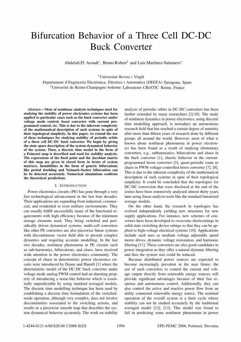
Let us consider the three-cell DC-DC buck converterpresented in Fig. 1. Each pair formed by a switch Si anda diode Di is activated in a complementary manner sothat when Si is ON, Di is OFF and vice versa. Becauseof the presence of switched elements such as MOSFETSand diodes, this system is a switched and usually it is aperiodically driven dynamical system with discontinuousvector field. Its structure changes cyclically when someconditions on the state variables and/or time are fulfilled.Let us suppose that the switching from one configurationCk to another one Ck+1 forms a well determined and fixed

vo

S1S2

D1

R

Vin

u1 u2

iL

vC,1

S3

D2 D3

Co

L

vC,2C1 C2

u3

iref

kv,2

Switching

Decision

u2

u3

iL

0.5vC,1

s2

s3

kv,1

Output voltage

controller

vo

Vref

-+

0.66Vin

vC,1

vC,2

ki

u1s1

Vo

ltag

e D

ivid

er

-+

-+

Fig. 1. Three-cell DC-DC buck converter and its PWM con-troller.

sequence:

C1 → C2 → . . . CM → C1 → C2 → . . . CM . . . (1)

During each configuration, the system is governed by alinear time invariant (LTI) equation of the following form

Configuration Ck : x = Akx + Bk := fk(x)for k = 1, 2 . . . M

(2)

where x ∈ R4 is the vector of state variables, A ∈ R

4×4

and B ∈ R4×1 are the system matrices and vectors during

each phase whose components are the system parametersR, L, Ck, Co and Vin. M is the number of configurationsused in a switching cycle and it depends on the duty cycleof the command signals. In order to obtain the equationsdescribing the dynamical behavior of the converter, weuse the standard Kirchhoff laws. For instance, for oursystem the modelling steps are as follows:

The current in the output capacitor is equal tothe difference between the inductor current iLand the load current. Therefore we have:

dvo

dt= − vo

RCo+

iLCo

(3)

The voltage vs,k across the switch Sk is ex-pressed as the product of the command signal uk

and the voltage difference between two adjacentcapacitors:

vs,k = uk(vc,k−1 − vc,k), vc,0 = Vin, vc,3 = 0(4)

where uk = 1 − uk and uk is the binarycommand signal for the kth switch that takesvalues in the set 0, 1.The current in the flying capacitors are de-termined as the time derivative of the voltageacross these capacitors multiplied by the capac-itance Ck:

iC,k = Ckdvc,k

dt= iL (uk − uk+1) (5)

1995

RVin

iL

vC,1 Co

L

vC,2C1 C2vo RVin

iL

vC,1 Co

L

vC,2

C1

C2

vo

R

iL

vC,2 Co

vC,1

C2 vo

LC1

R

iL

vC,1 Co

L

C1 voVin

Vin

R

iLvC,1

Co

L

vC,2

C1 C2

Vin vo R

iLvC,1

Co

C1 C2

Vin vo

vC,2

R

iL

Co

L

vC,1 vC,2C1

R

iL

vC,1 Co

L

C1

C2

voVin

vC,2

Vin

vC,2

vo

(a)

(c)

(g)

(e)

(b)

(d)

(h)

(f)

C2

C2

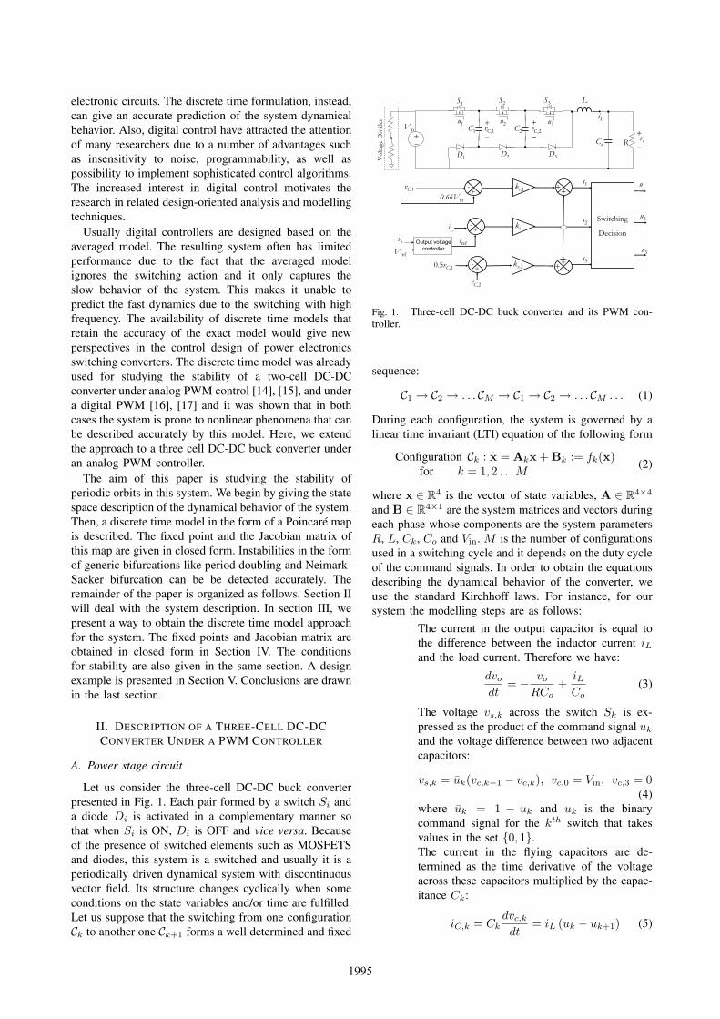
Fig. 2. Basic configurations for a three cell DC-DC buckconverter. (a) Configuration C1 (ON,ON,ON), (b) Configura-tion C2 (ON,ON,OFF) (c) Configuration C3 (ON,OFF,OFF),(d) Configuration C4 (OFF,OFF,OFF), (e) Configuration C5

(OFF,ON,ON), (f) Configuration C6 (OFF,OFF,ON), (g) Config-uration C7 (OFF,ON,OFF), (h) Configuration C8 (ON,OFF,ON).

and the voltage across the inductance is givenby the product of this inductance and the timederivative of the inductor current iL:

LdiLdt

= Vin −3∑

k=1

vs,k − vo (6)

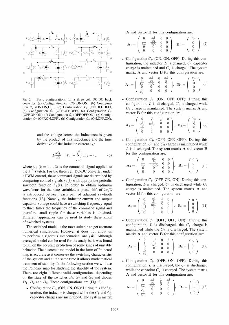
where uk (k = 1 . . . 3) is the command signal applied tothe kth switch. For the three cell DC-DC converter undera PWM control, these command signals are determined bycomparing control signals sk(t) with appropriate periodicsawtooth function hk(t). In order to obtain optimumwaveforms for the state variables, a phase shift of 2π/3is introduced between each pair of adjacent sawtoothfunctions [13]. Namely, the inductor current and outputcapacitor voltage could have a switching frequency equalto three times the frequency of the command signal andtherefore small ripple for these variables is obtained.Different approaches can be used to study these kindsof switched systems.

The switched model is the most suitable to get accuratenumerical simulations. However it does not allow usto perform a rigorous mathematical analysis. Althoughaveraged model can be used for the analysis, it was foundto fail on the accurate prediction of some kinds of unstablebehavior. The discrete time model in the form of Poincarémap is accurate as it conserves the switching characteristicof the system and at the same time it allows mathematicaltreatment of stability. In the following section we will usethe Poincaré map for studying the stability of the system.There are eight different valid configurations dependingon the state of the switches S1, S2 and S3 and diodesD1, D2 and D3. These configurations are (Fig. 2):

• Configuration C1, (ON, ON, ON): During this config-uration, the inductor is charged while the C1 and C2

capacitor charges are maintained. The system matrix

A and vector B for this configuration are:

A1 =

⎛⎜⎜⎝

0 −1L

0 01

Co

−1RCo

0 00 0 0 00 0 0 0

⎞⎟⎟⎠ B1 =

⎛⎜⎝

VinL000

⎞⎟⎠ (7)

• Configuration C2, (ON, ON, OFF): During this con-figuration, the inductor L is charged, C1 capacitorcharge is maintained and C2 is charged. The systemmatrix A and vector B for this configuration are:

A2 =

⎛⎜⎜⎝

0 −1L

0 −1L

1Co

−1RCo

0 00 0 0 01

C20 0 0

⎞⎟⎟⎠ B2 =

⎛⎜⎝

VinL000

⎞⎟⎠ (8)

• Configuration C3, (ON, OFF, OFF): During thisconfiguration, L is discharged, C1 is charged whileC2 charge is maintained. The system matrix A andvector B for this configuration are:

A3 =

⎛⎜⎜⎝

0 −1L

−1L

01

Co

−1RCo

0 01

C10 0 0

0 0 0 0

⎞⎟⎟⎠ B3 =

⎛⎜⎝

VinL000

⎞⎟⎠ (9)

• Configuration C4, (OFF, OFF, OFF): During thisconfiguration, C1 and C2 charge is maintained whileL is discharged. The system matrix A and vector Bfor this configuration are:

A4 =

⎛⎜⎜⎝

0 −1L

0 01

Co− 1

RCo0 0

0 0 0 00 0 0 0

⎞⎟⎟⎠ B4 =

⎛⎜⎝

0000

⎞⎟⎠ (10)

• Configuration C5, (OFF, ON, ON): During this con-figuration, L is charged, C1 is discharged while C2

charge is maintained. The system matrix A andvector B for this configuration are:

A5 =

⎛⎜⎜⎝

0 −1L

1L

01

Co

−1RCo

0 0−1C1

0 0 00 0 0 0

⎞⎟⎟⎠ B5 =

⎛⎜⎝

0000

⎞⎟⎠ (11)

• Configuration C6, (OFF, OFF, ON): During thisconfiguration, L is discharged, the C1 charge ismaintained while the C2 is discharged. The systemmatrix A and vector B for this configuration are:

A6 =

⎛⎜⎜⎝

0 −1L

0 1L

1Co

−1RCo

0 00 0 0 0−1C2

0 0 0

⎞⎟⎟⎠ B6 =

⎛⎜⎝

0000

⎞⎟⎠ (12)

• Configuration C7, (OFF, ON, OFF): During thisconfiguration, L is discharged, the C1 is dischargedwhile the capacitor C2 is charged. The system matrixA and vector B for this configuration are:

A7 =

⎛⎜⎜⎝

0 −1L

1L

−1L

1Co

−1RCo

0 0−1C1

0 0 01

C20 0 0

⎞⎟⎟⎠ B7 =

⎛⎜⎝

0000

⎞⎟⎠ (13)

,

,

,

,

,

,

,

1996

u1

Timeu2

Switching period

Timeu3

Time

C7 C5 C6 C8 C3 C2

0 t1 t3 t5 T

0

1

0

0

1

1

0

0

1

1

0

1

1

0

0

1

1

0

3

T 2

3

T

Fig. 3. The three command signals for the three-cell buckconverter for a duty cycle 33% 66% and phase shiftequal to 2 3.

• Configuration C8, (ON, OFF, ON): During this con-figuration, L is charged, capacitor C2 are dischargedwhile C1 charge is charged. The system matrix Aand vector B for this configuration are:

A8 =

⎛⎜⎜⎝

0 −1L

−1L

1L

1Co

−1RCo

0 01

C10 0 0

−1C2

0 0 0

⎞⎟⎟⎠ B8 =

⎛⎜⎝

VinL000

⎞⎟⎠(14)

Different sequences are possible depending on the dutycycle of the command signal and phase shift among them.These sequences define different operating mode of theconverter. Hereafter, and without loss of generality, wewill focus on a duty cycle 33% < d < 66% and phaseshift equal to 2π/3. The switching sequence in this casewill be the following: C7 → C5 → C6 → C8 → C3 →C2, which corresponds to (u1, u2, u3)= (0, 1, 0), (0, 1, 1)(0, 0, 1), (1, 0, 1), (1, 0, 0) and (1, 1, 0) . This sequencegives rise to a periodic orbit with six configurations duringone switching cycle. Figure 3 shows the three commandsignals u1, u2 and u3 corresponding to this sequence.

B. PWM Controller

In order to perform the switch mode operation of theconverter and with the purpose of regulating the outputvoltage vo and the flying capacitor voltages vc,1 andvc,2, the duty cycles of the command signals must becontrolled. Pulse Width Modulation technique plays therole of the basic control method. In the traditional PWMcontrol, the duty cycles of the command signals u1, u2

and u3 are varied according to the error signals to controlthe output signals. The simplest analog form of generatingfixed frequency PWM is by comparison with a linearslope waveform such as a triangular periodic signal insuch a way that the output signal goes high/low when thecontrol signal is higher/lower than the triangular signal.This is implemented using a comparator whose outputvoltage goes to a logic one when one input is greater thanthe other. Other signals with straight edges can be used

for modulation. A falling ramp carrier will generate PWMwith leading edge modulation. When the control signal sk

is smaller (resp. greater) than the sawtooth ramp voltagehk, the switch is OFF (resp. ON). As the system containsthree controlled switches, this modulation strategy shouldbe applied for the three switches. The ramp carriers arephase shifted in such a way that the control signal s1 iscompared with the ramp carrier signal h1(t), the controlsignal s2 is compared with h2(t) = h1(t − T

3 ) whilethe signal s3 is compared with the sawtooth ramp signalh3(t) = h1(t − 2T

3 ), where T is the period of the rampsignal which coincides with the switching period. In thecase of a digital PWM control this will be also thesampling period. Obtaining the expression of the controlsignals is challenging as the system is multi-input multi-output (MIMO).

A MIMO control design may be the work of anotherresearch in this area and it is beyond the scope of thispaper. We will consider here a purely proportional controlwith the aim to minimize the error between the outputsand their references values.

In order to control the voltage vC,1 to 2Vin/3, iLto iref and vC,2 to Vin/3 we consider the error signalse1 = 2Vin/3 − vC,1, e2 = (iref − iL) and e3 = (vc,2 −0.5vC,1). Then the control signals to be compared withthe repetitive signals hk are as follows:

s1(x) = kv,1e1 + kie2

s2(x) = kie2

s3(x) = kv,2e3 + kie2

(15)

where ki, kv,1 and kv,2 are feedback coefficients. It isworth noting here that due to the phase shift among therepetitive signals hk, two of the switching instants aresynchronous and are given in a fixed pattern. These aret2 = T/3 and t4 = 2T/3. The other remaining switchinginstants are asynchronous and they are obtained as thesolution of the equation resulting from the crossing of thecontrol signals sk with the ramp periodic functions hk.These periodic functions have the following expressions:

h1(t) = Vu − (V u − V l) tT mod 1

h2(t) = Vu − (V u − V l) t−T/3T mod 1

h3(t) = Vu − (V u − V l) t−2T/3T mod 1

(16)

In order to get output voltage regulation the signal irefis taken from the output voltage controller. If a purelyproportional controller is used, this reference current isgiven by:

iref = ko(Vref − vo) (17)

where ko is the proportional gain.

III. DISCRETE TIME MODELLING

A. Poincaré Map of periodic orbits

Following a procedure similar to that used in [14], adiscrete time model can be obtained for the system. Thismap relates the state variable at the nth cycle to those atthe n + 1st cycle. From this map, the stationary periodicorbits are located and their stability is studied by studyingthe local behavior of the map.

< d </π

,

1997

The usefulness of the Poincaré map results from thefact that its fixed points X∗ correspond to periodic orbitsx∗ of the continuous time switched system and that thestability properties are the same for both of them. Thepiecewise affine character of this class of systems allowsus to obtain the fixed points of P in terms of time instantstk. Generally, function ϕk can be written as:

ϕk(t,xk−1) = φk(t)xk−1 + ψk(t)Bk (18)

where matrices φ and ψ are given as follows:

φ(t) = eAt, ψ(t) =∫ t

0

eAαdα (19)

Note that the matrix ψ is well defined by Equation (19)even if A is singular. If A is invertible, the matrixfunction ψ can be written as:

ψ(t) = A−1 (φ(t) − 1) (20)

where 1 is the identity matrix with appropriate dimension.In the case of a singular matrix A, we have from (19) andusing time series expansion of the matrix exponential:

ψ(t) =(1t +

At2

2+

A2t3

6+ . . . +

Aktk+1

(k + 1)!+ . . .

)(21)

Independently of wether A is invertible or not, the expres-sion of map P can be written in the following form: Ifwe collect the time durations of each configuration dk ina column vector d = (d1, d2, . . . dM )t and perform somealgebra,we obtain that the expression of the map functionP can be written as follows:

P(xn,d) = Φ(d)xn + Ψ(d) (22)

where

Φ(d) =∏1

k=M k( k)

Ψ(d) =∑M−1

j=1

∏j+1k=M k( k) j( j)Bj + M ( M )BM

1 = 1

k = k − k−1 for 2 − 1 andM = − M−1

B. Fixed Points

A fixed point of P is a point X∗ in the state space forwhich we have X∗ = P(X∗,d∗). Using the expression ofP, X∗ can be expressed in terms of the vector of steadystate time durations d∗, corresponding to fixed points X∗,and matrices Φ and Ψ evaluated at d∗, i.e:

X∗(d∗) = (1 − Φ(d∗))−1 · Ψ(d∗) (23)

It should be noted here that the fixed point and hence itsassociated periodic orbit exists and it is unique wheneverthe inverse in (23) exists, i.e. if the matrix (1 − Φ(d∗))is not singular.

C. Orbital Stability Analysis

The stability of periodic orbits x∗ is the same as thatof fixed points X∗ of the map P. This can be investigatedusing the Jacobian matrix DP of this map. The piecewiseaffinity and time invariance of the system during eachsub-interval allows the obtaining of DP in closed formin terms of tk. If all these instants are given in a fixedpattern, the system will be open loop system, and DPcan be expressed as the product of the Jacobian matrixof each local map. By differentiating (22), we obtain thatthe Jacobian matrix DP is

DP = Φ(d) (24)

It can be noted that, in this case, a sufficient but notnecessary condition to assure the asymptotic stability ofthe switched system is that each affine configuration isasymptotically stable. That is to say, if all matrices Ak

have all eigenvalues in the left half side of the complexplane, all the eigenvalues of Φ(d∗) will be inside theunit circle. In closed loop systems, some of the timeinstants tk depend on the state variables linearly or bysome nonlinear form depending on the controller. Let ussuppose that, in the closed loop system, the switchingfunctions σk defining the switching manifolds Σk canbe written as the difference between a state dependentfunction sk(x) and a time dependent T -periodic functionhk as it is the case for analog PWM controllers. In thiscase we have:

Σk =

x ∈ Rn

/σk(x, t) := sk(x) − hk(t) = 0

(25)

Generally, functions sk defining the switching manifoldsΣk could take any form. However, for a typical linearfeedback controller, they are linear functions of the errorsof the state variables and, thus, they can be written assk(x) = Kk(Xref,k−x), where Kk are suitable feedbackcoefficients during the switching kth sub-interval that areselected with the purpose to control some output variablesand Xref,k is the vector of the reference trajectory in thekth sub-interval. The functions hk are, without loss ofgenerality, piecewise linear T -periodic signals of time thatare used together with the error signals to get a desiredstationary average value of the output variables and thedesired switching period T for the state variables. Notethat as the switching condition is given by a nonlinearequation, there can exist more than one set of switchinginstants and therefore more than one periodic orbit. Next,we focus on the presence of a periodic orbit for the systemin closed loop. Given such a periodic orbit, the switchinginstants in each period, determined by the feedback, arefixed in steady state.

Once these fixed instants are known, the associatedperiodic orbit can be computed. Hence, the stationaryswitching instants are determined by the associated pe-riodic orbit through the applied switching functions, andconversely, the stationary switching instants determine theperiodic orbit. Therefore, in order to compute the periodicorbit and the associated stationary switching instants, we

φ

ψddφ ψ

d

d

ddd

< k <M

t

t t

T t

1998

have to find a solution for a set of transcendental equationsconsisting of the equations imposed by the stationaryorbit that depend on the stationary switching instants,and Equation (23) by which the stationary switchinginstants can be obtained from the feedback (Equation(25)). As these equations are nonlinear, it turns out thatdepending on the value of the parameters there can bemore than one periodic orbit, some of which would notbe necessarily stable. Moreover, the stability issue is herea local matter. Usually, it is not possible to obtain a closedform expression for the stationary switching instants andtherefore for the corresponding fixed points. Obtaining thefixed point X∗ requires, therefore, solving a set of tran-scendental equations σ(X∗, τ∗) = 0 where the switchingvector function σ is given as the difference between theswitching signals sk and the repetitive periodic signalshk: σ = [s1 − h1 s2 − h2 s3 − h3]t. Therefore, aroot finding algorithm should be applied to the switchingcondition to obtain τ∗ = (t∗1, t∗2, ... , t∗5). For instance,the least squares method can be used. The problem canbe treated as an optimization process where the objectivefunction to be minimized is σ(τ∗) and the parameters tobe optimized are switching time instants tk, (k = 1...5),with the constraints 0 < tk < T . The process can bestarted from 5 equidistant switching instants in the interval(0, T ), i.e: τ0 =

(T6 , T

3 , ...5T6

)t. The optimal solution

τ∗ for the vector of switching instants τ = (t1, t2, ...t5)t

is then substituted in (23) to obtain the fixed point X∗.Recall that t∗2 and t∗4 are given in a fixed pattern. Oncethe fixed point is located, its stability analysis may becarried out by studying the local behavior of the map Pin its vicinity. In the closed loop system, some of theswitching time instants tk depend on the discrete statevariables xn in a nonlinear form. The dependence of theseinstants on the discrete state variables changes the natureof the map P from a linear map to a nonlinear one. Theexpression of the Jacobian matrix DP is also modifiedby the presence of terms containing the derivative of thevector of switching instants τ with respect to the vector ofthe discrete state variables xn. In this case the expressionof the Jacobian matrix becomes

DP = Φ(d) +∂P∂τ

∂τ

∂xn(26)

Note that, as the open loop system is stable, it is thesecond term in the expression of the Jacobian matrix thatcould introduce instability into the system. This fact canbe explored in designing a stable closed loop system byadjusting the parameters appearing in this term in orderto make it as small as possible. It is worth mentioninghere that in the case of a digital controller, closed formexpression of τ in terms of xn is available and thenexplicit differentiation of τ with respect to xn is possible.If an analog controller is used, as it is the case on thispaper, explicit differentiation of τ with respect to xn is notpossible. However, the implicit function theorem allowsus to write:

∂τ

∂xn= −

(∂σ

∂τ

)−1∂σ

∂xn(27)

Then the expression of DP becomes

DP = Φ(d) − ∂P∂τ

(∂σ

∂τ

)−1∂σ

∂xn(28)

By differentiating the vector of switching functions σ withrespect to xn we obtain the partial derivative of σ withrespect to the state variables. Likewise by differentiating σwith respect to τ we obtain the partial derivative of σ withrespect to the switching instants. Note that as the vectorfield is discontinuous, the state variables derivative x−

k

just before switching are different from the derivatives x+k

just after switching. If such discontinuities do not exist,the matrix ∂σ

∂τ will be diagonal. Finally, partial derivativeof the map function P with respect to τ can be obtainedin the same way.

The stability analysis of the nominal periodic orbit ofthe closed loop system, represented by X∗, can be carriedout by using the eigenvalues of DP evaluated at the fixedpoint X∗. This can be done by solving the characteristicequation for the fixed point X∗ which is given by:

det(DP − λ1) = 0 (29)

A well known condition for instability is that one ofthe eigenvalues has a modulus grater than 1. In thenext section, we will use the discrete time model of thesystem to study the stability of periodic orbits and theirpossible bifurcations. Readers interested in how to obtainthe expression of the Poincaré map function, the fixedpoints and its Jacobian matrix can read [18].

IV. RESULTS

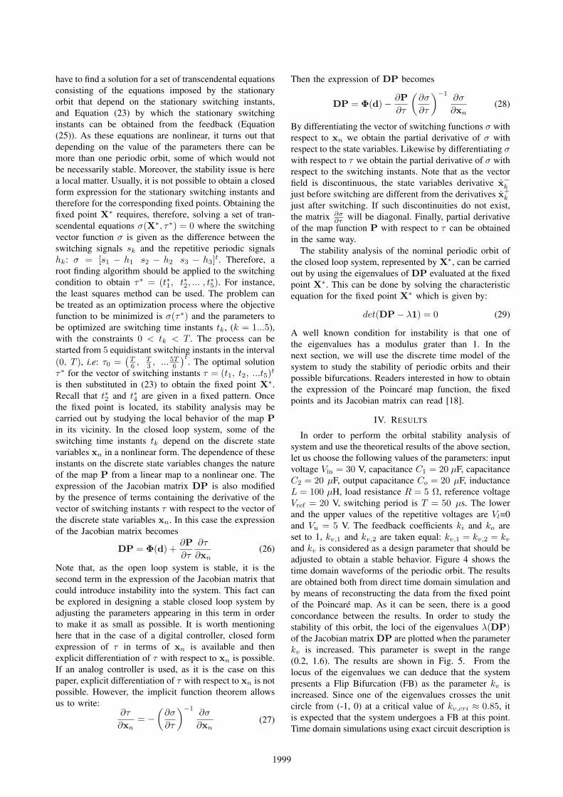
In order to perform the orbital stability analysis ofsystem and use the theoretical results of the above section,let us choose the following values of the parameters: inputvoltage Vin = 30 V, capacitance C1 = 20 µF, capacitanceC2 = 20 µF, output capacitance Co = 20 µF, inductanceL = 100 µH, load resistance R = 5 Ω, reference voltageVref = 20 V, switching period is T = 50 µs. The lowerand the upper values of the repetitive voltages are Vl=0and Vu = 5 V. The feedback coefficients ki and ko areset to 1, kv,1 and kv,2 are taken equal: kv,1 = kv,2 = kv

and kv is considered as a design parameter that should beadjusted to obtain a stable behavior. Figure 4 shows thetime domain waveforms of the periodic orbit. The resultsare obtained both from direct time domain simulation andby means of reconstructing the data from the fixed pointof the Poincaré map. As it can be seen, there is a goodconcordance between the results. In order to study thestability of this orbit, the loci of the eigenvalues λ(DP)of the Jacobian matrix DP are plotted when the parameterkv is increased. This parameter is swept in the range(0.2, 1.6). The results are shown in Fig. 5. From thelocus of the eigenvalues we can deduce that the systempresents a Flip Bifurcation (FB) as the parameter kv isincreased. Since one of the eigenvalues crosses the unitcircle from (-1, 0) at a critical value of kv,cri ≈ 0.85, itis expected that the system undergoes a FB at this point.Time domain simulations using exact circuit description is

1999

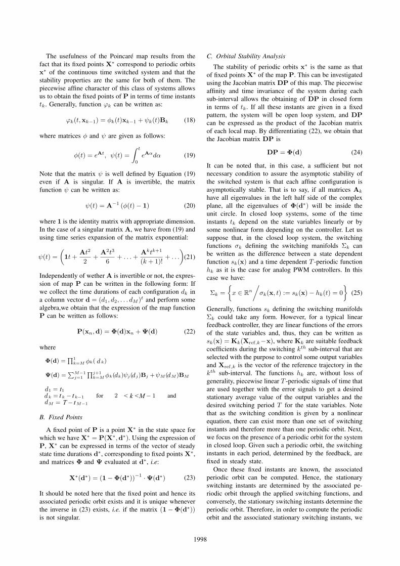
(a)

0.8 0.82 0.84 0.86 0.88 0.9 0.92 0.94 0.96 0.98 12.5

3

3.5

i L

0.8 0.82 0.84 0.86 0.88 0.9 0.92 0.94 0.96 0.98 114.8

14.9

15

v o

0.8 0.82 0.84 0.86 0.88 0.9 0.92 0.94 0.96 0.98 119

20

21

22

v c,1

0.8 0.82 0.84 0.86 0.88 0.9 0.92 0.94 0.96 0.98 18

9

10

11

Time/ms

v c,2

(b)

0 0.005 0.01 0.015 0.02 0.025 0.03 0.035 0.04 0.045 0.052.5

3

3.5

Time/ms

iL

0 0.005 0.01 0.015 0.02 0.025 0.03 0.035 0.04 0.045 0.0514.8

14.9

15

Time/ms

vo

0 0.005 0.01 0.015 0.02 0.025 0.03 0.035 0.04 0.045 0.0519

20

21

22

Time/ms

vc,1

0 0.005 0.01 0.015 0.02 0.025 0.03 0.035 0.04 0.045 0.058

9

10

11

Time/ms

vc,2

C7

C5 C

6C8 C

3C2

Fig. 4. Stationary periodic waveforms of the state variables. (a)from simulation of the switched model during four switchingperiods (transient should be removed). (b) from the reconstruc-tion of the fixed point of the Poincaré map

−1.5 −1 −0.5 0 0.5 1 1.5−1.5

−1

−0.5

0

0.5

1

1.5

Real part: Re(λ)

Imag

inar

y pa

rt: I

m(λ

)

Unit circle

kv,cri Increasing k

v

º open loop eigenvalues. closed loop eigenvalues

Fig. 5. Eigenvalues loci of the Jacobian matrix of the Poincarémap corresponding to the three cell DC-DC buck converter asthe parameter v is increased. The eigenvalues of the open loopsystem are also indicated by small circles.

0.2 0.4 0.6 0.8 1 1.2 1.4 1.60

1

2

3

4

5

6

7

Bifurcation parameter kv

Sam

pled

indu

ctor

cur

rent

iL(n

T)

FB

BC

T−periodic2T−periodic

Chaos

Fig. 6. Bifurcation diagram taking v as a bifurcation parametershowing a FB.

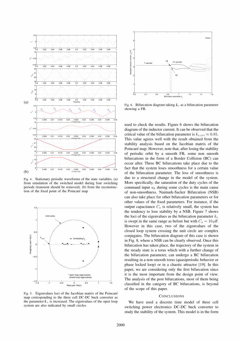
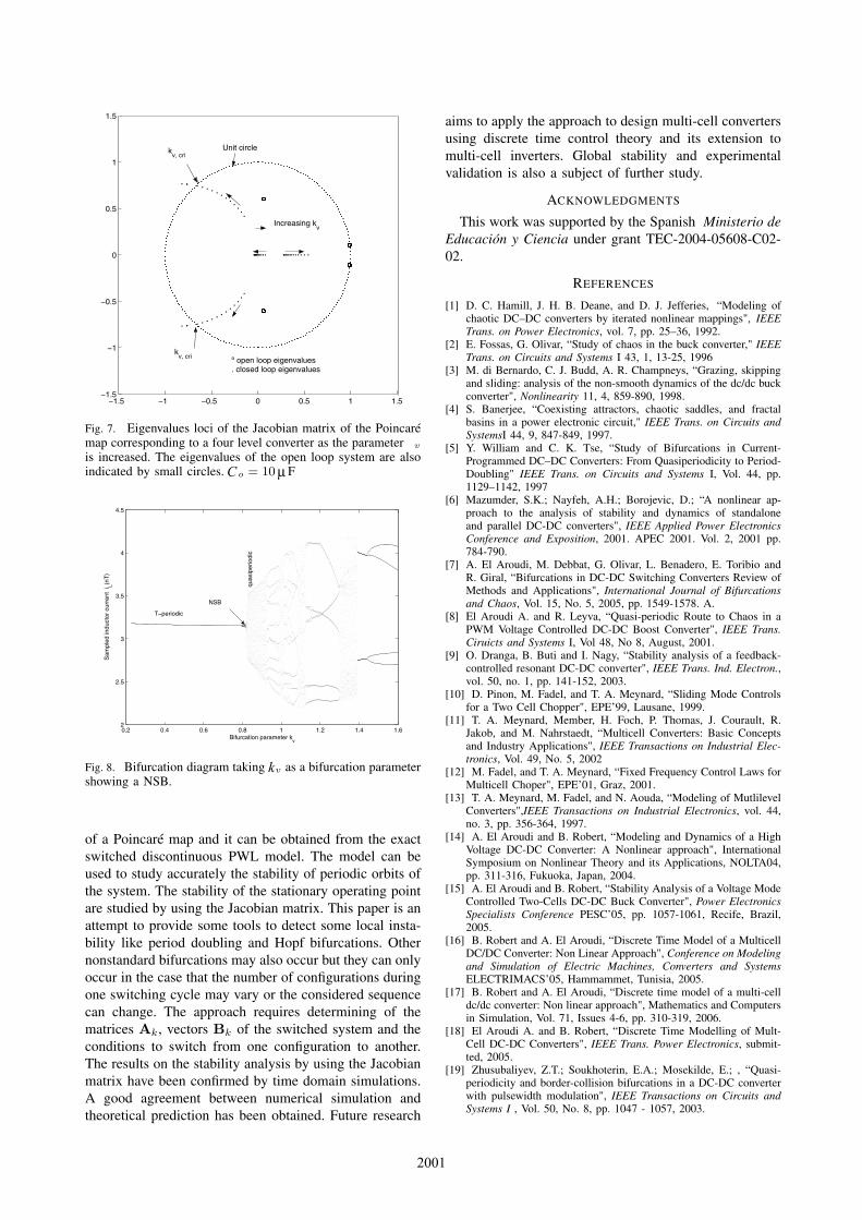
used to check the results. Figure 6 shows the bifurcationdiagram of the inductor current. It can be observed that thecritical value of the bifurcation parameter is kv,cri ≈ 0.85.This value agrees well with the result obtained from thestability analysis based on the Jacobian matrix of thePoincaré map. However, note that, after losing the stabilityof periodic orbit by a smooth FB, some non smoothbifurcations in the form of a Border Collision (BC) canoccur after. These BC bifurcations take place due to thefact that the system loses smoothness for a certain valueof the bifurcation parameter. The loss of smoothness isdue to a structural change in the model of the system.More specifically, the saturation of the duty cycles of thecommand input uk during some cycles is the main causeof non-smoothness. Naimark-Sacker Bifurcation (NSB)can also take place for other bifurcation parameters or forother values of the fixed parameters. For instance, if theoutput capacitance Co is relatively small, the system hasthe tendency to lose stability by a NSB. Figure 7 showsthe loci of the eigenvalues as the bifurcation parameter kv

is swept in the same range as before but with Co = 10µF.However in this case, two of the eigenvalues of theclosed loop system crossing the unit circle are complexconjugates. The bifurcation diagram of this case is shownin Fig. 8, where a NSB can be clearly observed. Once thisbifurcation has taken place, the trajectory of the system inthe steady state is a torus which with a further change ofthe bifurcation parameter, can undergo a BC bifurcationresulting in a non-smooth torus (quasiperiodic behavior orphase locked loop) or in a chaotic attractor [19]. In thispaper, we are considering only the first bifurcation sinceit is the most important from the design point of view.The analysis of the post bifurcations, most of them beingclassified in the category of BC bifurcations, is beyondof the scope of this paper.

CONCLUSIONS

We have used a discrete time model of three cellswitching power electronics DC-DC buck converter tostudy the stability of the system. This model is in the form

k

k

2000

−1.5 −1 −0.5 0 0.5 1 1.5−1.5

−1

−0.5

0

0.5

1

1.5

Unit circle

º open loop eigenvalues. closed loop eigenvalues

Increasing kv

kv, cri

kv, cri

Fig. 7. Eigenvalues loci of the Jacobian matrix of the Poincarémap corresponding to a four level converter as the parameter v

is increased. The eigenvalues of the open loop system are alsoindicated by small circles. o = 10 F

0.2 0.4 0.6 0.8 1 1.2 1.4 1.62

2.5

3

3.5

4

4.5

Bifurcation parameter kv

Sam

pled

indu

ctor

cur

rent

iL(n

T)

NSB

T−periodic

quas

iper

iodi

c

Fig. 8. Bifurcation diagram taking v as a bifurcation parametershowing a NSB.

of a Poincaré map and it can be obtained from the exactswitched discontinuous PWL model. The model can beused to study accurately the stability of periodic orbits ofthe system. The stability of the stationary operating pointare studied by using the Jacobian matrix. This paper is anattempt to provide some tools to detect some local insta-bility like period doubling and Hopf bifurcations. Othernonstandard bifurcations may also occur but they can onlyoccur in the case that the number of configurations duringone switching cycle may vary or the considered sequencecan change. The approach requires determining of thematrices Ak, vectors Bk of the switched system and theconditions to switch from one configuration to another.The results on the stability analysis by using the Jacobianmatrix have been confirmed by time domain simulations.A good agreement between numerical simulation andtheoretical prediction has been obtained. Future research

aims to apply the approach to design multi-cell convertersusing discrete time control theory and its extension tomulti-cell inverters. Global stability and experimentalvalidation is also a subject of further study.

ACKNOWLEDGMENTS

This work was supported by the Spanish Ministerio deEducación y Ciencia under grant TEC-2004-05608-C02-02.

REFERENCES

[1] D. C. Hamill, J. H. B. Deane, and D. J. Jefferies, “Modeling ofchaotic DC–DC converters by iterated nonlinear mappings", IEEETrans. on Power Electronics, vol. 7, pp. 25–36, 1992.

[2] E. Fossas, G. Olivar, “Study of chaos in the buck converter," IEEETrans. on Circuits and Systems I 43, 1, 13-25, 1996

[3] M. di Bernardo, C. J. Budd, A. R. Champneys, “Grazing, skippingand sliding: analysis of the non-smooth dynamics of the dc/dc buckconverter", Nonlinearity 11, 4, 859-890, 1998.

[4] S. Banerjee, “Coexisting attractors, chaotic saddles, and fractalbasins in a power electronic circuit," IEEE Trans. on Circuits andSystemsI 44, 9, 847-849, 1997.

[5] Y. William and C. K. Tse, “Study of Bifurcations in Current-Programmed DC–DC Converters: From Quasiperiodicity to Period-Doubling" IEEE Trans. on Circuits and Systems I, Vol. 44, pp.1129–1142, 1997

[6] Mazumder, S.K.; Nayfeh, A.H.; Borojevic, D.; “A nonlinear ap-proach to the analysis of stability and dynamics of standaloneand parallel DC-DC converters", IEEE Applied Power ElectronicsConference and Exposition, 2001. APEC 2001. Vol. 2, 2001 pp.784-790.

[7] A. El Aroudi, M. Debbat, G. Olivar, L. Benadero, E. Toribio andR. Giral, “Bifurcations in DC-DC Switching Converters Review ofMethods and Applications", International Journal of Bifurcationsand Chaos, Vol. 15, No. 5, 2005, pp. 1549-1578. A.

[8] El Aroudi A. and R. Leyva, “Quasi-periodic Route to Chaos in aPWM Voltage Controlled DC-DC Boost Converter", IEEE Trans.Ciruicts and Systems I, Vol 48, No 8, August, 2001.

[9] O. Dranga, B. Buti and I. Nagy, “Stability analysis of a feedback-controlled resonant DC-DC converter", IEEE Trans. Ind. Electron.,vol. 50, no. 1, pp. 141-152, 2003.

[10] D. Pinon, M. Fadel, and T. A. Meynard, “Sliding Mode Controlsfor a Two Cell Chopper", EPE’99, Lausane, 1999.

[11] T. A. Meynard, Member, H. Foch, P. Thomas, J. Courault, R.Jakob, and M. Nahrstaedt, “Multicell Converters: Basic Conceptsand Industry Applications", IEEE Transactions on Industrial Elec-tronics, Vol. 49, No. 5, 2002

[12] M. Fadel, and T. A. Meynard, “Fixed Frequency Control Laws forMulticell Choper", EPE’01, Graz, 2001.

[13] T. A. Meynard, M. Fadel, and N. Aouda, “Modeling of MutlilevelConverters",IEEE Transactions on Industrial Electronics, vol. 44,no. 3, pp. 356-364, 1997.

[14] A. El Aroudi and B. Robert, “Modeling and Dynamics of a HighVoltage DC-DC Converter: A Nonlinear approach", InternationalSymposium on Nonlinear Theory and its Applications, NOLTA04,pp. 311-316, Fukuoka, Japan, 2004.

[15] A. El Aroudi and B. Robert, “Stability Analysis of a Voltage ModeControlled Two-Cells DC-DC Buck Converter", Power ElectronicsSpecialists Conference PESC’05, pp. 1057-1061, Recife, Brazil,2005.

[16] B. Robert and A. El Aroudi, “Discrete Time Model of a MulticellDC/DC Converter: Non Linear Approach", Conference on Modelingand Simulation of Electric Machines, Converters and SystemsELECTRIMACS’05, Hammammet, Tunisia, 2005.

[17] B. Robert and A. El Aroudi, “Discrete time model of a multi-celldc/dc converter: Non linear approach", Mathematics and Computersin Simulation, Vol. 71, Issues 4-6, pp. 310-319, 2006.

[18] El Aroudi A. and B. Robert, “Discrete Time Modelling of Mult-Cell DC-DC Converters", IEEE Trans. Power Electronics, submit-ted, 2005.

[19] Zhusubaliyev, Z.T.; Soukhoterin, E.A.; Mosekilde, E.; , “Quasi-periodicity and border-collision bifurcations in a DC-DC converterwith pulsewidth modulation", IEEE Transactions on Circuits andSystems I , Vol. 50, No. 8, pp. 1047 - 1057, 2003.

C

k

µ

2001