ON THE USE OF NEWTON’S ROOTFINDINGALGORITHM FOR SOLVING THE RANS EQUATIONS

Aldo BonfiglioliUniversita degli Studi della Basilicata, Potenza, Italy

Abstract

Viene descritta l’implementazione dell’algoritmo di Newton per risolvere i sistemi diequazioni algebriche non-lineari che si ottengo dalla discretizzazione delle equazioni dellafluidodinamica. In particolare, vengono studiate le equazioni di Navier-Stokes medialea la Reynolds-Favre (RANSE) in cui la turbolenza e descritta tramite il modello ad unaequazione dovuto a Spalart e Allmaras. Le applicazioni considerate, entrambe bidimen-sionali, riguardano il flusso attraverso una schiera anulare di turbina, International Stan-dard Configuration 11 (STCF 11), ed il flusso esterno attorno al profilo RAE 2822. Ven-gono confermate le eccellenti qualita di convergenza dell’algoritmo che non solo consentedi raggiungere la soluzione stazionaria in poche decine di iterazioni non-lineari, ma in-oltre permette di raggiungere livelli di convergenza dell’ordine dello zero macchina, dif-ficilmente ottenibili utilizzando metodi iterativi meno sofisticati. D’altro canto, vengonoevidenziati alcuni limiti dell’implementazione descritta.

1 Introduction

Despite a widespread feeling that only unstructured grid schemes provide sufficient ver-satility to handle complex geometries and allow automatic mesh adaptation, shade is stillbeing cast about the ability of unstructured grid schemes to provide accurate results forboundary layer flows, especially if triangular/tetrahedral meshes are employed within thelayer. Although the use of hybrid grids, with hexahedra being used in the near wall region,might somewhat alleviate the problem, it is questionable, for example, how to (automat-ically) construct hexahedral cells within detached shear layers, eventually rolling up intomore complex fluid structures. Therefore, the right question to be posed is rather how toconstruct accurate unstructured schemes for high Reynolds’ number Navier-Stokes calcu-lation on truely unstructured grids.

Two different strategies addressing this issue can be identified in the literature over re-cent years: one of these advocates the use of truely multidimensional physical models whileretaining a low order (linear) representation of the dependent variables, the other still re-lies on the one-dimensional Riemann model commonly used in state-of-the-art CFD codes,but employs higher order polynomial representation of the unknowns. The DiscountinuousGalerkin (DG) method belongs to this latter class and has gained considerable attentionover recent years by showing impressively detailed results on coarse (by Finite Volume(FV) standards) meshes. The DG method inherits from the Finite Element (FE) methodthe flexibility in handling complex geometries and the ease in increasing polynomial orderby swithching between different element types. It also borrows ideas from the FV setting,

1

most notably the use of (approximate) Riemann solvers to compute a single valued inviscidflux function at the interface between adjacent elements, where the data representation is,by contruction, discontinuous. Following very similar ideas, higher order FV methods haveappeared in the literature, showing a good degree of success. Similarly to the DG method,higher order interpolants are constructed locally which are discontinuous across the con-trol volume boundaries. Contrary to the DG method, in which higher order elements areobtained by adding degrees of freedom within a cell, the FV higher order polynomial re-construction requires an enlarged computational stencil as informations are gathered fromat least two rows of cell neighbours to construct a quadratic interpolant. The price to bepaid for the gain in accuracy is both increased computational cost and memory storage, andboth increase quite dramatically as the polynomial order is increased.

Improving accuracy while retaining reasonable computational cost might be achievedby improving the numerical model; this can be achieved by abandoning the one-dimensional,grid-aligned models, and introducing truely multi-dimensional ones. The numerical methodto be described in the present paper belongs to this latter class and was originally intro-duced by Roe in the early eighties and named “fluctuation splitting”, also often referred toas ”residual distribution”. Since then, the methodology has greatly evolved thanks to thecontributions of several research groups worldwide and has nowadays reached a sufficientdegree of maturity to allow routine calculations of complex flows. A critical comparisonwith state-of-the-art FV techniques has been recently presented by the VKI group. It isshown in () that MD schemes greatly reduce the amount of spurious diffusion over stan-dard FV schemes when first order schemes are compared. For second order schemes, theimprovement is not so remarkable, althoud MD schemes allow to achieve a comparableaccuracy on a more compact stencil and with better monotonicity preserving properties.Moreover, margins of improvement appear to be available for MD schemes, along with thepossibility to adopt higher order interpolants at reasonable additional cost. Both issues havebeen addressed in recent works, although these have been demonstrated only for relativelysimple flows.

The increased computational cost inevitably incurred by more complex numerical mod-els can be largely compensated if the new model also allows to improve the convergencecharacteristics of the numerical algorithm. A considerable effort has been made by variousauthors over recent years to improve the convergence characteristics of CFD solvers forsteady flows, by separating the acoustic from the advective components of the subsonic,steady Euler equations and using the most appropriate discretization technique for eachof the two. Although these pioneering efforts have demonstrated an impressive potential,much work still needs to be done to extend these ideas to the Navier-Stokes equations.

The present paper deals with the issue of convergence acceleration for steady, high-Reynolds’ number flows. Multi-dimensional ”fluctuation splitting” schemes are used todiscretize the Reynolds’ averaged Navier-Stokes (RANS) equations, and convergence ac-celeration is achieved using a “brute force” approach which consists in applying Newton’srootfinding method to the large and sparse system of non-linear equations which is obtainedafter discretization of the governing conservation equations.

Although not widespreadly used, Newton’s method is certainly not new in the CFDarena and has also been previously applied by others and the author in conjunction with FSschemes as well. The present paper addresses specific issues related to the solution of theRANS equations.

The paper is organized as follows. Sect. 2 recalls the basic characteristics of the spatialdiscretazion schemes for both the mean flow and turbulent transport equations. In Sect. 3Newton’s algorithm is discussed along the features and problems peculiar to the solution ofthe RANS equations. Its application to an internal and an external flow configuration are

2

reported in Sect. 4.

2 The numerical method

The conservation law form of the RANS equations can be written as follows∫

CV

∂U

∂tdV +

∫

CS

(Fcn + F

vn) dS = 0 (1)

where CS is the control surface bounding the control volume CV , which we shall considerfixed in space, and F

cn and F

vn denote, respectively, the convective and diffusive fluxes

through the infinitesimal surface element of area dS and unit normal n. Eq. (1) allowsto deal with both compressible and incompressible (constant density) flows if Chorin’s (1)artificial compressibility approach is use for the the latter.

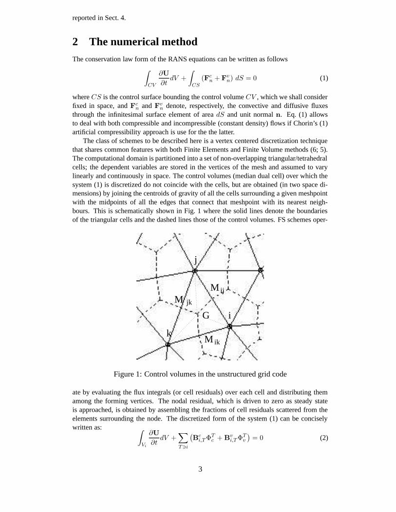
The class of schemes to be described here is a vertex centered discretization techniquethat shares common features with both Finite Elements and Finite Volume methods (6; 5).The computational domain is partitioned into a set of non-overlapping triangular/tetrahedralcells; the dependent variables are stored in the vertices of the mesh and assumed to varylinearly and continuously in space. The control volumes (median dual cell) over which thesystem (1) is discretized do not coincide with the cells, but are obtained (in two space di-mensions) by joining the centroids of gravity of all the cells surrounding a given meshpointwith the midpoints of all the edges that connect that meshpoint with its nearest neigh-bours. This is schematically shown in Fig. 1 where the solid lines denote the boundariesof the triangular cells and the dashed lines those of the control volumes. FS schemes oper-

i

j

k

G

M jk

M ij

ikM

Figure 1: Control volumes in the unstructured grid code

ate by evaluating the flux integrals (or cell residuals) over each cell and distributing themamong the forming vertices. The nodal residual, which is driven to zero as steady stateis approached, is obtained by assembling the fractions of cell residuals scattered from theelements surrounding the node. The discretized form of the system (1) can be conciselywritten as:

∫

Vi

∂U

∂tdV +

∑

T3i

(

Bci,T ΦT

c + Bvi,T ΦT

v

)

= 0 (2)

3

where Vi is the control volume centered about meshpoint i and the summation extends overthe cells T sharing meshpoint i. The matrices B

ci,T and B

vi,T are used to distribute the

convective and diffusive residuals (or fluctuations):

ΦTc =

∫

T

FcndS ΦT

v =

∫

T

FvndS.

The distribution of the viscous fluxes can be shown to be equivalent to a standard FE dis-cretization, while the inviscid fluxes are distributed in an upwind-biased fashion. Contraryto most FV schemes, no Riemann problems are involved since the functional representationof the dependent variables is continuous across the elements. The generalized upwindingdirections are based upon the eigenstructure of the quasi-linear form of the inviscid com-ponent of the equations.

Another key ingredient of the method consist in the fact that the inviscid flux balance iscomputed using the quasi-linear form of the equations, so that the fluxes are never actuallycomputed. A suitable choice of the set of dependent variable guarantees conservation andgives the method shock capturing capabilities.

Although the details of the discretization are given in fuller details elsewhere, see (3), abrief account of the discretization of the inviscid component of the equations is given herefor completeness.

It can be shown that the flux balance (or fluctuation) over a (triangular/tetrahedral) cellT can be computed as:

ΦTc =

d+1∑

i=1

KTi Ui

Ui being the nodal value of the conserved variables in the i-th vertex of the cell. The so-called “generalized inflow parameter” Ki (the superscript T will be dropped from now onto alleviate the notation) is proportional to jacobian matrix of the inviscid fluxes ni beingthe normal to the face opposite vertex i, scaled by its measure and pointing inside the cell.The factor of proportionality is the measure of the side/face opposite vertex i divided bythe dimension of the space, d:

Ki =1

d|ni|Ani

Since the Euler equations are hyperbolic in time, matrix Anihas real eigenvalues and a

complete set of eigenvectors so that it can be split into positive and negative parts using theeigenvector decomposition:

A±ni

= RniΛ

±ni

Lni(3)

where Λ±ni

is a diagonal matrix whose entries are the positive/negative eigenvalues of A±ni

and Rniand Lni

the matrices of the right and left eigenvectors. Various schemes can bebuild upon the splitting defined by Eq. (3). The N (Narrow) and LDA (Low Diffusion-A)schemes are among the most widely used. For these two, the fraction of the cell fluctuationsent to vertex i takes the form:

ΦNi = −K

+

i (Ui −U−)

ΦLDAi = ∆

+

i Φc

where:

∆±

i =

(

d+1∑

`=1

K±

`

)−1

K±

i U− =

d+1∑

`=1

∆`U`.

While closed form expressions for the matrices K±

i can be computed (see, e.g. Eq. 8 forthe compressible case), small dense linear systems of order equal to the number of degrees

4

of freedom in each gridpoint need to be solved numerically to compute the ∆i matrices andthe so-called inflow point U− within each cell.

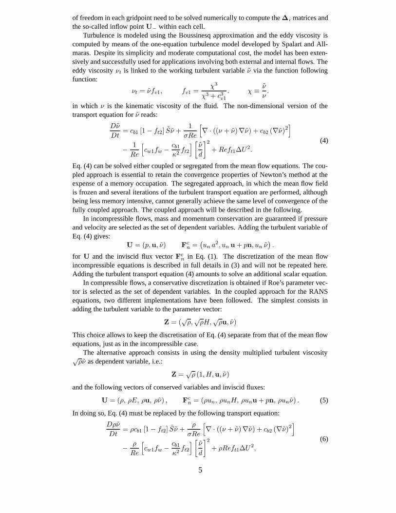
Turbulence is modeled using the Boussinesq approximation and the eddy viscosity iscomputed by means of the one-equation turbulence model developed by Spalart and All-maras. Despite its simplicity and moderate computational cost, the model has been exten-sively and successfully used for applications involving both external and internal flows. Theeddy viscosity νt is linked to the working turbulent variable ν via the function followingfunction:

νt = νfv1, fv1 =χ3

χ3 + c3v1

. χ ≡ ν

ν.

in which ν is the kinematic viscosity of the fluid. The non-dimensional version of thetransport equation for ν reads:

Dν

Dt= cb1 [1 − ft2] Sν +

1

σRe

[

∇ · ((ν + ν)∇ν) + cb2 (∇ν)2]

− 1

Re

[

cw1fw − cb1

κ2ft2

]

[

ν

d

]2

+ Reft1∆U2.

(4)

Eq. (4) can be solved either coupled or segregated from the mean flow equations. The cou-pled approach is essential to retain the convergence properties of Newton’s method at theexpense of a memory occupation. The segregated approach, in which the mean flow fieldis frozen and several iterations of the turbulent transport equation are performed, althoughbeing less memory intensive, cannot generally achieve the same level of convergence of thefully coupled approach. The coupled approach will be described in the following.

In incompressible flows, mass and momentum conservation are guaranteed if pressureand velocity are selected as the set of dependent variables. Adding the turbulent variable ofEq. (4) gives:

U = (p,u, ν) Fcn =

(

un a2, un u + pn, un ν)

.

for U and the inviscid flux vector Fcn in Eq. (1). The discretization of the mean flow

incompressible equations is described in full details in (3) and will not be repeated here.Adding the turbulent transport equation (4) amounts to solve an additional scalar equation.

In compressible flows, a conservative discretization is obtained if Roe’s parameter vec-tor is selected as the set of dependent variables. In the coupled approach for the RANSequations, two different implementations have been followed. The simplest consists inadding the turbulent variable to the parameter vector:

Z = (√

ρ,√

ρH,√

ρu, ν)

This choice allows to keep the discretisation of Eq. (4) separate from that of the mean flowequations, just as in the incompressible case.

The alternative approach consists in using the density multiplied turbulent viscosity√ρν as dependent variable, i.e.:

Z =√

ρ (1,H,u, ν)

and the following vectors of conserved variables and inviscid fluxes:

U = (ρ, ρE, ρu, ρν) , Fcn = (ρun, ρunH, ρunu + pn, ρunν) . (5)

In doing so, Eq. (4) must be replaced by the following transport equation:

Dρν

Dt= ρcb1 [1 − ft2] Sν +

ρ

σRe

[

∇ · ((ν + ν)∇ν) + cb2 (∇ν)2]

− ρ

Re

[

cw1fw − cb1

κ2ft2

]

[

ν

d

]2

+ ρReft1∆U2,

(6)

5

in which the molecular turbulent viscosity appears as the transported scalar. The jacobianmatrix An = ∂F

cn/∂U of the inviscid fluxes, Eq. (5), reads:

An =

0 0 nt 0

[−H + (γ − 1) k]un γun Hnt − (γ − 1) unu

t 0−uun + (γ − 1) kn (γ − 1)n un− (γ − 1)nu + unI 0

−unν 0 νnt un

(7)

The eigenvalues of matrix (7) are:

λ0 = un = u · n (multiplicity d+2) λ± = un±a

a being the sound speed. Positive and negative parts of matrix (7) can be computed accord-ing to equation (3):

A±n =

a±11

a±12

a±13

0a±

21a±

22(a±

23)t 0

a±

31a±

32A

±

330

a±61

a±62

a±

63a±

66

(8)

The individual entries of matrix (8), which have been represented for compactness asscalars (such as a11), vectors (such as a31, superscript t stands for transpose) or tensorsor order 2 (A33), can be computed explicitly and are reported in the Appendix.

3 Newton’s algorithm

Newton’s rootfinding algorithm is a well known and powerful tool for finding the zeroesof a non-linear equation or system of equations. It is however computationally quite cum-bersome as it requires knowledge of the jacobian matrix of the system of equations to besolved. When complex numerical models are employed and moreover when turbulencemodels are included, this can easily become untractable by analytical means. In the presentcontext, the jacobian matrix is computed by one-sided finite differences and stored in mem-ory. Due to the compactness of the schemes, whose stencil never extends beyond the set ofnearest neighbours, the memory requirement for the storage of the jacobian matrix is keptto a minimum, though it is still remarkable also because a second matrix with at least thesame sparsity pattern is required as a preconditioner for the iterative linear solver. Anotherfeature which turns out to be essential for enjoying all the desirable convergence char-acteristics of Newton’s algorithm is full coupling between the mean flow and turbulencetransport equations.

The discretization of the governing equations in space, see Eq. (2), leads to the follow-ing system of ordinary differential equations:

MdU

dt= R(U) (9)

where R represents the spatial discretization operator, or the “nodal” residual, which van-ishes at steady state and M the mass matrix. Since we are only interested in steady statesolutions, the mass matrix can be replaced by the diagonal matrix of the control volumes.If the time derivative in equation (9) is approximated using a two points, one-sided finitedifference:

dU

dt=

Un+1 −U

n

∆t,

6

then an explicit scheme is obtained by evaluating R(U) at time level n and an implicitscheme if R(U) is evaluated at time level n+1. In this latter case, linearizing R(U) abouttime level n, i.e.

R(U)n+1 = R(U)n +

(

∂R

∂U

)n(

Un+1 −U

n)

+ H.O.T.

we obtain the following implicit scheme:(

V

∆tI− ∂R

∂U

)

(

Un+1 −U

n)

= R(U). (10)

Equation (10) represents a large nonsymmetric (though structurally symmetric) sparse lin-ear system of equations to be solved at each time step for the updates of the vector ofprimitive variables. The linear system 10 is solved using the PETSc library (4). The term∂R∂U

is the jacobian of the residual. If we let ∆t → ∞, equation (10) approaches New-ton’s rootfinding method, which is known to yield quadratic convergence for an ”educated”initial guess. Thanks to the compact stencil of the schemes used, the graph of the jaco-bian matrix coincides with the graph of the underlying unstructured mesh, i.e. it onlyinvolves distance-1 neighbours. Neverthless, the analytical evaluation of the Jacobian ma-trix, though not impossible, is rather complicated and even more if a turbulence model isincluded. Therefore, the approach followed in the present work consists in constructingthe jacobian matrix by means of one-sided finite difference approximations. Although thisis quite simple from a programming viewpoint, it is also computationally quite expensive.The assembly of the jacobian matrix requires a loop over all elements in the mesh; withinevery element each degree of freedom of all vertices needs to be perturbed and the corre-sponding residual be evaluated. This totals to a numer of residual evaluations equal to theproduct of the number of vertices (i.e. d+1 for triangular/tetrahedral cells) in a cell timesthe number of degrees of freedom in each node (i.e. d+3 for compressible and d+2 forincompressible flows). The cost of a single matrix assembly is therefore equal to 12 or 15residual evaluations (or explicit iteration) in two space dimensions and up to 21 to 24 inthree space dimensions. This considerable cost for matrix assembly is therefore justifiedonly if the reduction over simpler implicit schemes in the number of non-linear iterationsrequired to reach convergence pays off. Whether this may be true or not, heavily dependsupon the initial solution. Newton’s method is know to converge rapidly if the initial guessis not too far from the steady solution. In CFD application, a good initial guess may beavailable if parametric studies are performed, but there will always be the need, at somestage, to start a new calculation from “scratch”. In inviscid and viscous laminar calcula-tions the freestream flow conditions proved to be an acceptable initial condition provideda finite time-step ∆t is employed in the early stages of the calculation. Tipically, ∆t iscomputed according to a CFL-like condition and then muliplied by the ratio between theL2-norm of the residuals at the first and current non-linear iteration:

∆t := ∆tR(U0)

R(Uk)

thus rapidly reaching very large values as the steady solution is approached. The additionof a non-zero diagonal term in Eq. (10) also improves the convergence characteristics ofthe iterative linear solver at each non-linear iteration. It is only in the last stages of theiterative process that the diagonal term in Eq. (10) becomes negligibly small and Newton’salgorithm is fully recovered. While this approach worked well for inviscid and viscouslaminar flows, it turned out to be far more problematic in turbulent flow calculations and

7

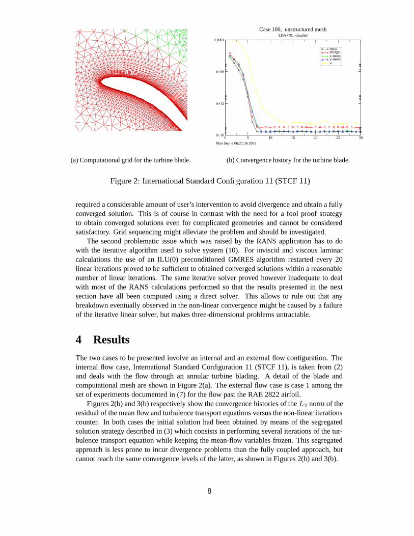
(a) Computational grid for the turbine blade.

0 5 10 15 20 25 301e-16

1e-12

1e-08

0,0001

massenergyx-momy-momν

Case 100, unstructured meshLDA+NL, coupled

Mon Sep 8 06:21:36 2003

(b) Convergence history for the turbine blade.

Figure 2: International Standard Configuration 11 (STCF 11)

required a considerable amount of user’s intervention to avoid divergence and obtain a fullyconverged solution. This is of course in contrast with the need for a fool proof strategyto obtain converged solutions even for complicated geometries and cannot be consideredsatisfactory. Grid sequencing might alleviate the problem and should be investigated.

The second problematic issue which was raised by the RANS application has to dowith the iterative algorithm used to solve system (10). For inviscid and viscous laminarcalculations the use of an ILU(0) preconditioned GMRES algorithm restarted every 20linear iterations proved to be sufficient to obtained converged solutions within a reasonablenumber of linear iterations. The same iterative solver proved however inadequate to dealwith most of the RANS calculations performed so that the results presented in the nextsection have all been computed using a direct solver. This allows to rule out that anybreakdown eventually observed in the non-linear convergence might be caused by a failureof the iterative linear solver, but makes three-dimensional problems untractable.

4 Results

The two cases to be presented involve an internal and an external flow configuration. Theinternal flow case, International Standard Configuration 11 (STCF 11), is taken from (2)and deals with the flow through an annular turbine blading. A detail of the blade andcomputational mesh are shown in Figure 2(a). The external flow case is case 1 among theset of experiments documented in (7) for the flow past the RAE 2822 airfoil.

Figures 2(b) and 3(b) respectively show the convergence histories of the L2 norm of theresidual of the mean flow and turbulence transport equations versus the non-linear iterationscounter. In both cases the initial solution had been obtained by means of the segregatedsolution strategy described in (3) which consists in performing several iterations of the tur-bulence transport equation while keeping the mean-flow variables frozen. This segregatedapproach is less prone to incur divergence problems than the fully coupled approach, butcannot reach the same convergence levels of the latter, as shown in Figures 2(b) and 3(b).

8

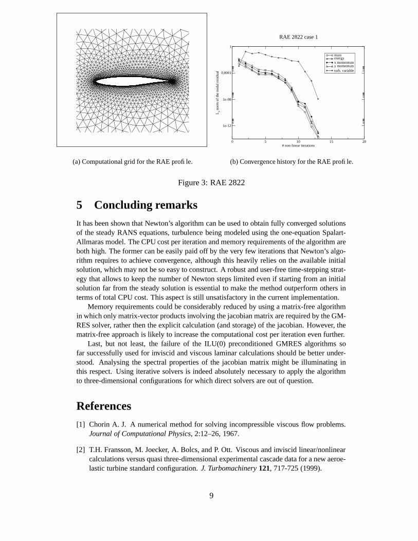
(a) Computational grid for the RAE profile.

0 5 10 15 20# non-linear iterations

1e-12

1e-08

0,0001

1

L2 n

orm

of

the

noda

l res

idua

l

massenergyx momentumy momentumturb. variable

RAE 2822 case 1

(b) Convergence history for the RAE profile.

Figure 3: RAE 2822

5 Concluding remarks

It has been shown that Newton’s algorithm can be used to obtain fully converged solutionsof the steady RANS equations, turbulence being modeled using the one-equation Spalart-Allmaras model. The CPU cost per iteration and memory requirements of the algorithm areboth high. The former can be easily paid off by the very few iterations that Newton’s algo-rithm requires to achieve convergence, although this heavily relies on the available initialsolution, which may not be so easy to construct. A robust and user-free time-stepping strat-egy that allows to keep the number of Newton steps limited even if starting from an initialsolution far from the steady solution is essential to make the method outperform others interms of total CPU cost. This aspect is still unsatisfactory in the current implementation.

Memory requirements could be considerably reduced by using a matrix-free algorithmin which only matrix-vector products involving the jacobian matrix are required by the GM-RES solver, rather then the explicit calculation (and storage) of the jacobian. However, thematrix-free approach is likely to increase the computational cost per iteration even further.

Last, but not least, the failure of the ILU(0) preconditioned GMRES algorithms sofar successfully used for inviscid and viscous laminar calculations should be better under-stood. Analysing the spectral properties of the jacobian matrix might be illuminating inthis respect. Using iterative solvers is indeed absolutely necessary to apply the algorithmto three-dimensional configurations for which direct solvers are out of question.

References

[1] Chorin A. J. A numerical method for solving incompressible viscous flow problems.Journal of Computational Physics, 2:12–26, 1967.

[2] T.H. Fransson, M. Joecker, A. Bolcs, and P. Ott. Viscous and inviscid linear/nonlinearcalculations versus quasi three-dimensional experimental cascade data for a new aeroe-lastic turbine standard configuration. J. Turbomachinery 121, 717-725 (1999).

9

[3] A. Bonfiglioli. Fluctuation splitting schemes for the compressible and incompressibleEuler and Navier-Stokes equations IJCFD, 14:21–39, 2000.

[4] PETSc home page http://www.mcs.anl.gov/petsc

[5] van der Weide E., Deconinck H., Issman E., Degrez G. A parallel, implicit, multi-dimensional upwind, residual distribution method for the Navier-Stokes equations onunstructured grids Computational Mechanics 23, 199-208 (1999).

[6] Deconinck H.,Paillere H.,Struijs R., P.L. Roe Multidimensional upwind schemes basedon fluctuation-splitting for systems of conservation laws, Computational Mechanics11, 323-340 (1993).

[7] AGARD report , 323-340 (1993).

10

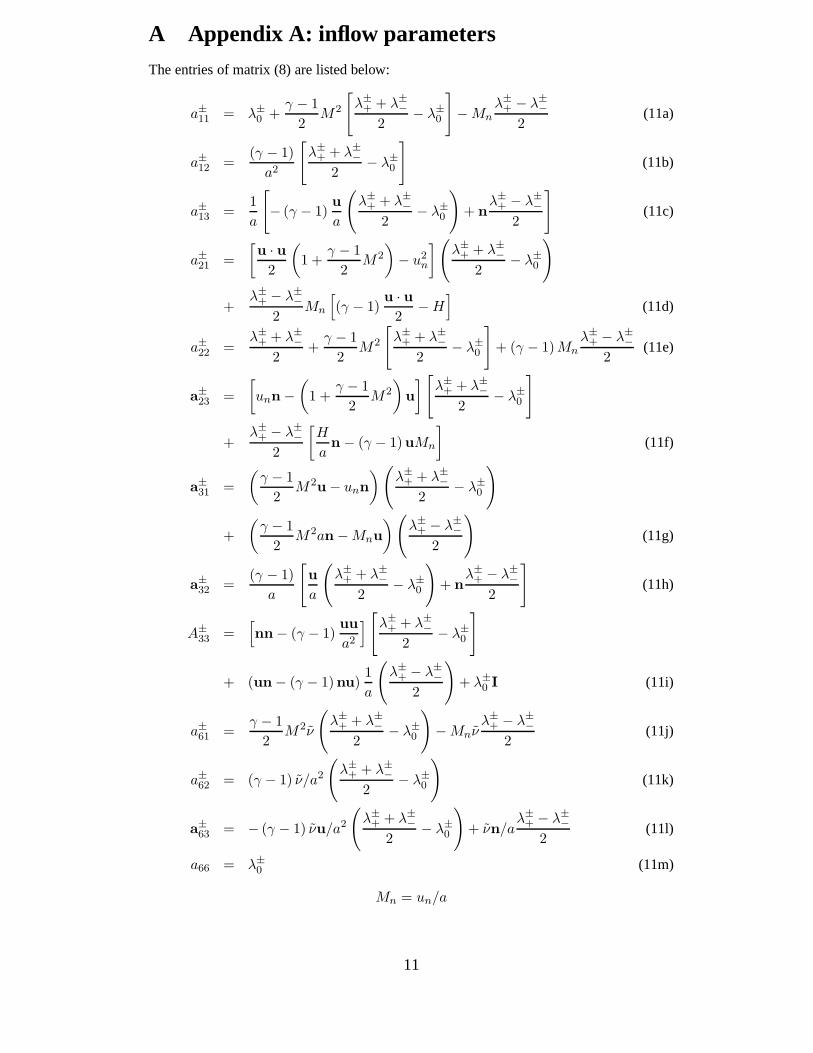
A Appendix A: inflow parameters

The entries of matrix (8) are listed below:

a±11

= λ±

0+

γ − 1

2M2

[

λ±+ + λ±

−

2− λ±

0

]

− Mn

λ±+ − λ±

−

2(11a)

a±12

=(γ − 1)

a2

[

λ±+ + λ±

−

2− λ±

0

]

(11b)

a±13

=1

a

[

− (γ − 1)u

a

(

λ±+ + λ±

−

2− λ±

0

)

+ nλ±

+ − λ±−

2

]

(11c)

a±21

=

[

u · u2

(

1 +γ − 1

2M2

)

− u2n

]

(

λ±+ + λ±

−

2− λ±

0

)

+λ±

+ − λ±−

2Mn

[

(γ − 1)u · u

2− H

]

(11d)

a±22

=λ±

+ + λ±−

2+

γ − 1

2M2

[

λ±+ + λ±

−

2− λ±

0

]

+ (γ − 1) Mn

λ±+ − λ±

−

2(11e)

a±

23=

[

unn−(

1 +γ − 1

2M2

)

u

]

[

λ±+ + λ±

−

2− λ±

0

]

+λ±

+ − λ±−

2

[

H

an − (γ − 1)uMn

]

(11f)

a±

31=

(

γ − 1

2M2

u − unn

)

(

λ±+ + λ±

−

2− λ±

0

)

+

(

γ − 1

2M2an − Mnu

)

(

λ±+ − λ±

−

2

)

(11g)

a±

32=

(γ − 1)

a

[

u

a

(

λ±+ + λ±

−

2− λ±

0

)

+ nλ±

+ − λ±−

2

]

(11h)

A±

33=

[

nn− (γ − 1)uu

a2

]

[

λ±+ + λ±

−

2− λ±

0

]

+ (un− (γ − 1)nu)1

a

(

λ±+ − λ±

−

2

)

+ λ±

0I (11i)

a±61

=γ − 1

2M2ν

(

λ±+ + λ±

−

2− λ±

0

)

− Mnνλ±

+ − λ±−

2(11j)

a±62

= (γ − 1) ν/a2

(

λ±+ + λ±

−

2− λ±

0

)

(11k)

a±

63= − (γ − 1) νu/a2

(

λ±+ + λ±

−

2− λ±

0

)

+ νn/aλ±

+ − λ±−

2(11l)

a66 = λ±

0(11m)

Mn = un/a

11