Chapter 6: Finding the Roots or

Solving Nonlinear Equations

Instructor: Dr. Ming Ye

Solving Nonlinear Equations and Sets of Linear Equations

• Equations can be solved analytically9Solution of y=mx+b9Solution of ax2+bx+c=0

• Large systems of linear equations• Higher order equations9Specific energy equation

• Nonlinear algebraic equations x=g(x)9Manning’s equation

Topics Covered in This Chapter

• Preliminaries• Fixed-Point Iteration• Bisection• Newton’s Method• The Secant Method• Hybrid Methods• Roots of Polynomials

Roots of f(x)=0

General Considerations• Is this a special function that will be evaluated often?

If so, some analytical study and possibly some algebraic manipulation of the function will be a good idea. Devise a custom iterative scheme.

• How much precision is needed?Engineering calculations often require only a few significant figures.

• How fast and robust must the method be?A robust procedure is relatively immune to the initial guess, and it converges quickly without being overly sensitive to the behavior of f(x) in the expected parameter space.

• Is the function a polynomial?There are special procedure for finding the roots of polynomials.

• Does the function have singularities?Some root finding procedures will converge to a singularity, as well as converge to a root.

There is no single root-finding method that is best for all situations.

The Basic Root-Finding Procedure

The basic strategy is1. Plot the function.

The plot provides an initial guess, and an indication of potential problems.

2. Select an initial guess.3. Iteratively refine the initial guess with a root-

finding algorithm.– The result is a sequence of values that, if all goes well,

get progressively closer to the root. – If xk is the estimate of the root, ξ, on the k-th iteration,

then the iterations converge if limk→∞xk=ξ.

-1.5 -1 -0.5 0 0.5 1 1.5-1.5

-1

-0.5

0

0.5

1

1.5

h (m)

f(h)

(m

3 )

The Basic Root-Finding Procedure

3. Iteratively refine the initial guess with a root-finding algorithm.– …

– For practical reasons, it is desirable that the root finder converges in as few steps as possible.

– Full automation of the root finding algorithm also requires a way to determine when to stop the iteration.

4. After a root has been found with an automatic root-finding procedure, it is a good idea to substitute the root back into the function to see whether f(x) ≈ 0.

Bracketing• Bracketing is a procedure to perform a coarse level search for roots

over a large interval on the x-axis.• The result is the identification of a set of subintervals that are likely to

contain roots.• Bracketing answers the question, “Where might the roots be?”• A root is bracketed on the interval [a, b] if f(a) and f(b) have opposite

sign. • A sign change occurs for singularities as well as roots.• Bracketing is used to make initial guesses at the roots, not to accurately

estimate the values of the roots.

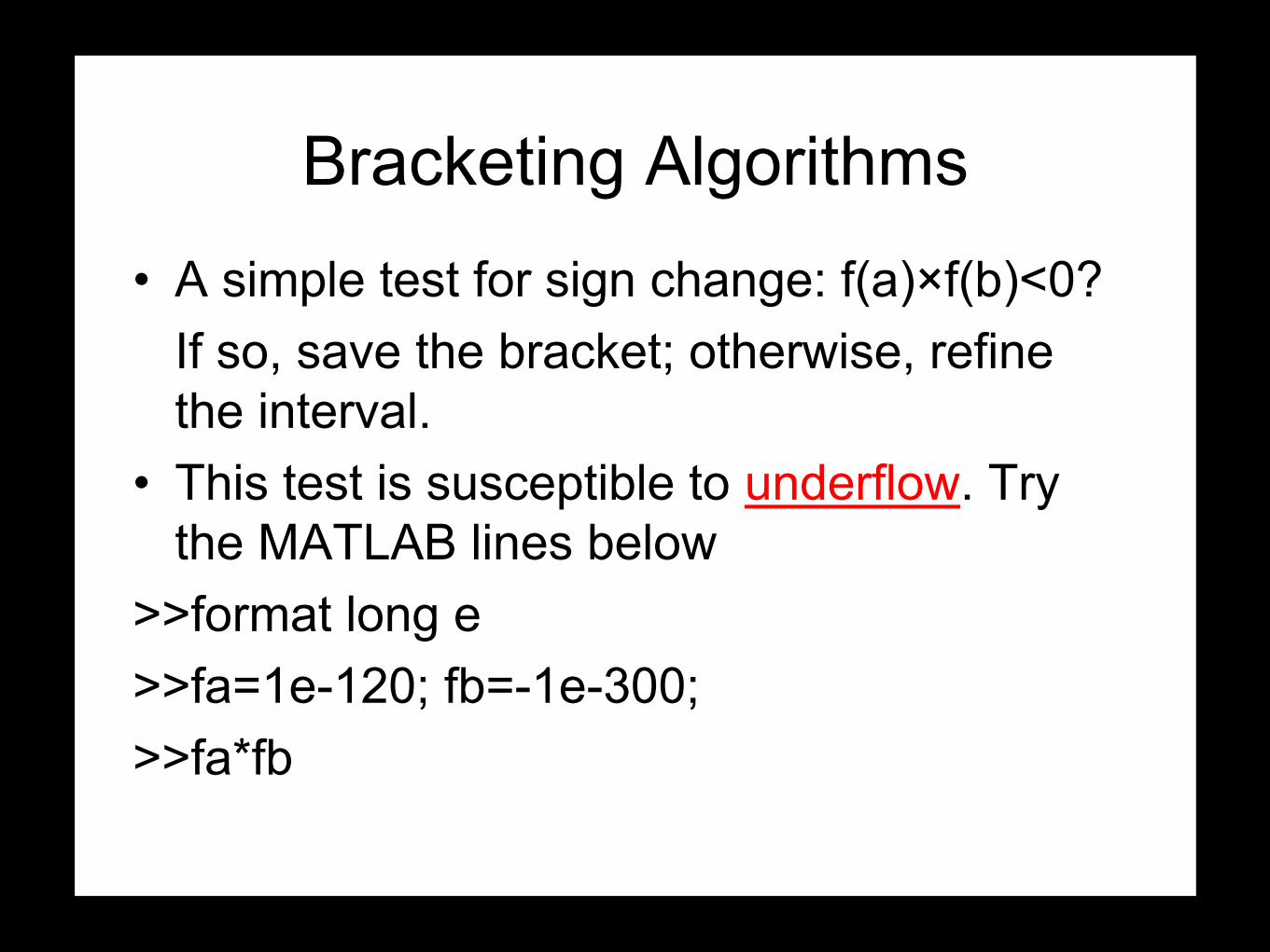
Bracketing Algorithms• A simple test for sign change: f(a)×f(b)<0?

If so, save the bracket; otherwise, refine the interval.

• This test is susceptible to underflow. Try the MATLAB lines below

>>format long e>>fa=1e-120; fb=-1e-300;>>fa*fb

Bracketing Algorithms

• This test is susceptible to underflow. Try the MATLAB lines below

>>format long e

>>fa=1e-120; fb=-1e-300;

>>fa*fb

• Solution:

>>sign(fa)~=sign(fb)

Root-Finding Algorithms

We now proceed to develop the following root-finding algorithms:

• Fixed point iteration• Bisection• Newton’s method• Secant methodThese algorithms are applied after initial

guesses at the root(s) are identified with bracketing (or guesswork).

Fixed-Point Iteration• Fixed point iteration is a simple method. It only works when the

iteration function is convergent.• As a simple root-finding procedure, fixed-point iteration is often used in

hand calculations.Given f(x) = 0, rewrite it as xnew = g(xold). a value of x that satisfies x=g(x)

will be a root of f(x).Algorithm:initialize: x0 = . . .for k = 1, 2, . . .xk = g(xk−1)if converged, stopend• Starting from an initial guess, x0, the iteration formula is simply:

x1 = g(x0), x2 = g(x1), …,xn+1 = g(xn), • You would hope that the sequence x0, x1, x2, … converges to the

solution x.• The fixed-point algorithm gets its name from its behavior at

convergence: recycling the output as input does not change the output. The root, ξ, is a fixed point of g(x).

Iterative Equations• There is generally more than one way in

which a function can be written in the form x = g(x).

• A problem one can run into with iterative solutions is finding a form of g(x) that will converge to any particular root.

Classroom Exercise

• f(x)=x2-2x-3=0• True solutions are x=-1 and x=3• x=g1(x)=sqrt(2x+3)• x=g2(x)=3/(x-2)• x=g3(x)=(x2-3)/2• Start from x0=4, solve up to x3.

Convergence of Fixed-Point Iteration

• Starting from an initial guess, x0, the iteration formula is

simply: x1

= g(x0), x2= g(x1), …,x

n+1= g(xn),

• The function g is evaluated with successive values of x until

xn+1- xn is as small as desired.

• You would hope that the sequence x0, x

1, x

2, … converges to

the solution x.

Analysis of fixed-point iteration reveals that the iterations are

convergent on the interval a≤x≤b if the interval contains a

root and if

^ `' ( ) 1, for all g x x a x b� � d d

If -1<g’(x)<0, the iterations oscillate while converging. If

0<g’(x)<1, the iterations converge monotonically.

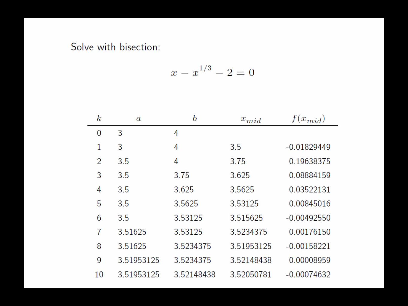
Bisection

• The logic: Given a bracketed root, repeatedly halve the interval while continue to bracket the root.

• Since the bracket is always reduced by a factor of two, bisection is sometimes called interval halving.

• Given the initial bracket [a,b], an improved approximation to the root is the midpoint of the interval xm=1/2(a+b).

• An alternative formula for the midpoint that is less susceptible to roundoff error is xm=a+1/2(b-a).

Algorithm

• Starting from x=a and x=b

• If f(x=a)*f(x=b)<0, then [a,b]

bracket the root

• The interval around the root is

halved successively until the

value of f(x) is close to 0

• With each halving, the root is

kept between the bracketing

values by paring the new value

with the previous value that

gives f(x) of the opposite sign.

• If f(x) is close enough to 0 or the

bracket values are close enough

with tolerance, stop.

ExerciseUse the figure below to explain how the bisection method works.

In comparison to the fixed point method, what are the pros and cons of the bisection method?

Bisection

• It is robust and, given initial values that bracket the root, the root will be found.

• In other words, bisection always converges if the original interval contained the root.

• It has the disadvantage of being slower to converge than many of the other methods.

• It is often used to find an approximate root to use as an initial value in some of the other more efficient techniques, such as Newton's method.

Analysis of Bisection

Convergence Criteria• An automatic root-finding procedure needs to

monitor progress toward the root and stop when current guess is close enough to the desired root.– It is extremely unlikely that a numerical procedure will

find the precise value of x that makes f(x) exactly zero in floating-point arithmetic.

– The algorithm must decide how close to the root the iteration should be before stopping the search.

• Convergence checking can consider whether two successive approximations to the root are close enough to be considered equal.

• Convergence checking can examine whether f(x) is sufficiently close to zero at the current guess.

Convergence Criteria• Convergence checking will avoid searching

to unnecessary accuracy.– As a practical consideration, it may not be

necessary to know the root to a large number of significant figures.

– Because the computer has finite resolution on the real number line, there is some limit below which refinements in the root cannot be made.

– Even if the true root is used to evaluate f(x), the result may not be zero, due to roundoff error.

Convergence Criteria• An automatic root-finding procedure needs to

monitor progress toward the root and stop when current guess is close enough to the desired root.

• Convergence checking will avoid searching to unnecessary accuracy.

• Two criteria can be applied in testing for convergence: – Check whether successive approximations are close

enough to be considered the same: |xk − xk−1|< δx– Check whether f(x) is close enough zero: |f(xk)| < δf– You need to specify the two tolerance.

Convergence Criteria on x

• You may choose the extreme value of δx=eps, the machine precision.

• The absolute tolerance is workable but highly restricted.• When |xk|>>1, the convergence test using the absolute tolerance

will never be satisfied, because the roundoff error in the subtraction of|xk-xk-1| will always be larger than the specified tolerance.

• The absolute error is useful when the limit of the iterative sequence is known to be near zero.

Convergence Criteria on x

• The relative tolerance is a measure of the relative reduction in the original bracket interval.

• The relative convergence criterion is always preferred, since it does not change if the problem is suitably scaled.

• In computer calculation, it is usually a good idea to report both relative and absolute errors.

Convergence Criteria on f(x)•Machine precision is the lower bound for both criteria. Using convergence criteria less than the machine precision may result in infinite loop.

•One way to specify the tolerances is to use multiples of εm.

•Extreme tight convergence criteria would be δx =5εmand δf =5εm.

Convergence Criteria on f(x)

ExerciseHow do you measure computational time of an algorithm?

The figures above demonstrate two situations:• The function value f(x) is insensitive to x, but the root is

sensitive.• The function value f(x) is sensitive to the x, but the root is

insensitive.Under the two circumstances, what is the conservative way to

choose the convergence criteria, tolerance on f(x) or ∆x?

Newton’s Method• Newton’s method,

sometimes called the Newton-Raphson method, uses information about the function, f(x), and its first derivative.

• Based on the idea that any function can be approximated by a straight line over some small interval – a fact that is taken advantage of over and over again in numerical solution techniques.

• Begin with an initial estimate x0 that is close to the real root.

A linear function

Solve the linear function

ExerciseExplain the figure for the Newton’s method

Algorithm:

What quantities do you need for implementing the Newton’s method?

Exercise

Solve 1/3( ) 2 0f x x x � �

using the Newton’s method by hand.Use x0=3 and calculate to x4.

Relation between Newton’s method and fix-point method?

1/3( ) 2 0f x x x � �

• Construct g3 function using the Newton’s method.• Write a MATLAB code to solve this problem.

Exercise

1/3

3 2/3

6 23

xgx�

�

�

Divergence of Newton’s Method

• If the first derivative of f(x) vanishes, then the procedure fails.

• Even though a good initial guess to the root is available, Newton’s method may diverge if the first derivative of the function approaches zero near the current estimate of the root.

Newton’s and Secant Methods

• Limitation:Newton's method generally works well for cases in which the derivative is known in advance, such as polynomials or other functions with straightforward derivatives.

• Secant methodUse finite difference to approximate the derivative at x0.

• The secant method uses the last two guesses at the root to estimate the slope.

Secant Method

• Analytical expression of f’(x) is unknown

• Starting from x1

• Approximate derivative by finite difference

for n=1, 2, 3…

ExerciseUse the figure to explain the algorithm.

Secant Method

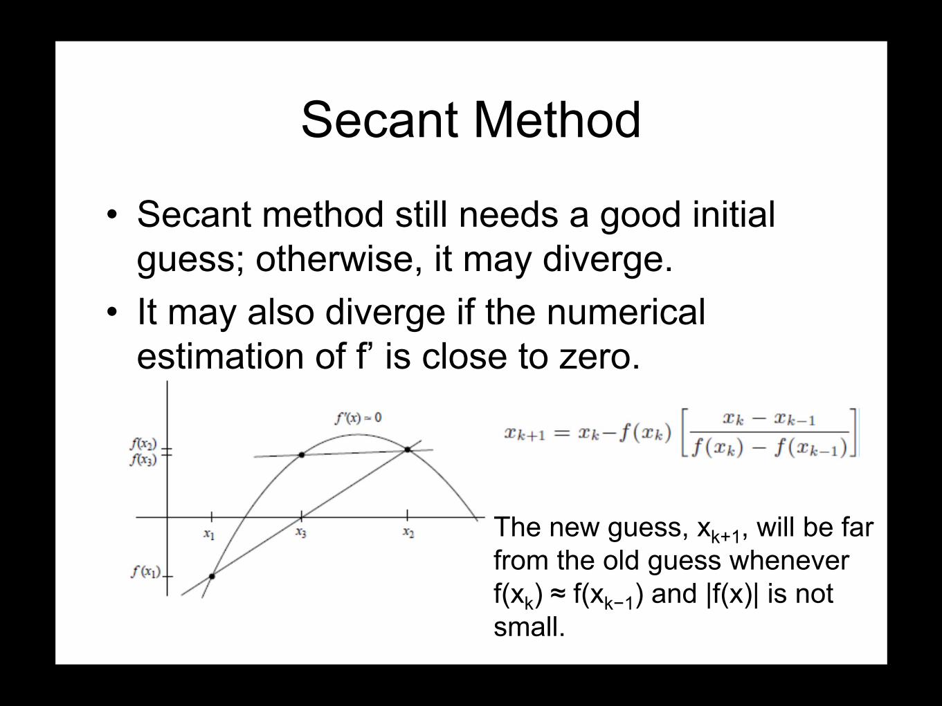
• Secant method still needs a good initial guess; otherwise, it may diverge.

• It may also diverge if the numerical estimation of f’ is close to zero.

The new guess, xk+1, will be far from the old guess whenever f(xk) ≈ f(xk−1) and |f(x)| is not small.

Classroom Exercise

1/3( ) 2 0f x x x � �

• Find the root using the Newton’s method for the initial guess of x1=4 and x2=3.

Take-Home Exercise

• Let f(x)=x2-6 and x0=1, use Newton’s method to find x2.

• Let f(x)=x2-6. With x0=3 and x1=2, use Secant method to find x2.

Summary of Basic Root-Finding Methods

• Plot f(x) before searching for roots• Bracketing finds coarse interval containing roots and

singularities• Bisection is robust, but converges slowly• Newton’s Method

– Requires f(x) and f′(x).– Iterates are not confined to initial bracket.– Converges rapidly.– Diverges if f′(x) ≈ 0 is encountered.

• Secant Method– Uses f(x) values to approximate f′(x).– Iterates are not confined to initial bracket.– Converges almost as rapidly as Newton’s method.– Diverges if f′(x) ≈ 0 is encountered.

Hybrid Methods• The root-finding methods discussed so far involve straightforward

iterative algorithms that are either robust (e.g., bisection) or converge rapidly (e.g., Newton’s method or the secant method).

• At the expense of increased programming logic, it is possible to combine these methods.

• A hybrid method might combine bisection with a more rapidly converging technique.

• At each iteration, a preliminary step of the faster method is taken. If the resulting estimate of the root is within the original bracket, then it is kept. Otherwise, a bisection step is taken.

• Such a hybrid algorithm converges no more slowly than bisection, and, with luck, it converges much more quickly.

• The advantage of a hybrid technique is that a rather coarse initial guess can be used at the root without worrying that the method will diverge.

The fzero Function

The fzero Function• fzero is a hybrid method that combines

bisection, secant and reverse quadratic interpolation

• Syntax:r = fzero(’fun’,x0)r = fzero(’fun’,x0,options)r = fzero(’fun’,x0,options,arg1,arg2,...)

• x0 can be a scalar or a two element vector• If x0 is a scalar, fzero tries to create its own

bracket.• If x0 is a two element vector, fzero uses the

vector as a bracket.

The fzero Function• Optional parameters to control fzero are specified with

the optimset function.Examples:• Tell fzero to display the results of each step:>> options = optimset(’Display’,’iter’);>> x = fzero(’myFun’,x0,options)• Tell fzero to use a relative tolerance of 5 × 10−9:>> options = optimset(’TolX’,5e-9);>> x = fzero(’myFun’,x0,options)• Tell fzero to suppress all printed output, and use a

relative tolerance of 5 × 10−4:>> options = optimset(’Display’,’off’,’TolX’,5e-4);>> x = fzero(’myFun’,x0,options)

The fzero Function

Classroom Exercise

Use fzero to solve 1/3( ) 2 0f x x x � �

(1) Use 0≤x≤5 as x0(2) Use x0=4.5

Roots of Polynomials

• The routines discussed up to this points can be applied to polynomials, because a polynomial in x can always be put in the form f(x)=0.

• These methods have difficulty due to – Repeated roots– Complex roots– Sensitivity of roots to small perturbations in

the polynomial coefficients (conditioning).

f1(x)=x2-3x+2: has two distinct rootsf2(x)=x2-10x+25: has repeated real rootsf3(x)=x2-17x+72.5: has complex roots

Algorithms for Finding Polynomial Roots

• To find the roots of a polynomial, it is better to use specialized numerical algorithms that are designed to deal with the complications:

• Bairstow’s method• Muller’s method• Laguerre’s method• Jenkin’s–Traub method• Companion matrix method

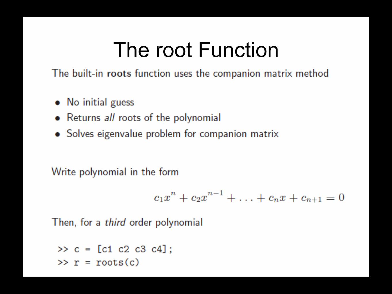
The root Function

Exercise

Use the roots function to find the roots of

Convergence Rates of Iterative Methods

• Unlike linear equations, most nonlinear equations cannot be solved in a finite number of steps.

• We must usually resort to an iterative method that produces increasingly accurate approximation to the solution, and we terminate the iteration when the result is sufficiently accurate.

• The total cost of solving the problem depends on both the cost per iteration and the number of iterations required for convergence, and there is often a trade-off between the two factors.

Rate of Convergence• http://en.wikipedia.org/wiki/Rate_of_convergence• In numerical analysis, the speed at which a convergent

sequence approaches its limit is called the rate of convergence.

• Although strictly speaking, a limit does not give information about any finite first part of the sequence, this concept is of practical importance if we deal with a sequence of successive approximations for an iterative method, as then typically fewer iterations are needed to yield a useful approximation if the rate of convergence is higher.

• This may even make the difference between needing ten or a million iterations.

Rate of Convergence• Suppose that the sequence {xk} converges

to the number L.• We say that this sequence converges

linearly to L, if there exists a number μ (0, 1) such that

• We say that the sequence converges with order q for q > 1 to L if

Convergence Rate• We denote the error at iteration k by ek, and it is usually

given by ek=xk-x*, where xk is the approximate solution at iteration k, and x* is the true solution.

• Some methods for one-dimensional problems do not actually produce a specific approximate solution xk, but merely an interval known to contain the solution, with the length of the interval decreasing as iterations proceed. For such methods, we take ek to be the length of the interval at iteration k.

• In either case, a method is said to converge with rate r if for some finite nonzero C.

• Some particular case of interest are these:– If r=1 and C<1, the convergence rate is linear.– If 1<r<2, the convergence rate is superlinear.– If r+2, the convergence rate is quadratic.

1lim krk

k

eC

e�

of

r=2

Convergence Rate• One way to interpret the distinction between linear and

superlinear convergence is that, asymptotically, a linear convergent sequence gains a constant number of digits of accuracy per iteration, whereas a superlinearly convergent sequence gains an increasing number of digits of accuracy with each iteration.

• Specially, a linearly convergent sequence gains –logβ(C) digits per iteration, but a superlinearly convergent sequence has r times as many digits of accuracy after each iteration as it has the previous iteration.

• In particular, a quadratically convergent method doubles the number of digits of accuracy with each iteration.

Exercise

• Why do we say that the bisection method has linear convergence rate?

• What is the convergence rate of the fix-point method?

Convergence Rate of Bisection Method• Suppose that the sequence {xk} converges to

the number L.• Determine the convergence rate by

examining

• But in the bisection method, we are not really interested in the solution xk but the interval when halving the original interval.

• Then, what is the convergence rate of the bisection method?

or

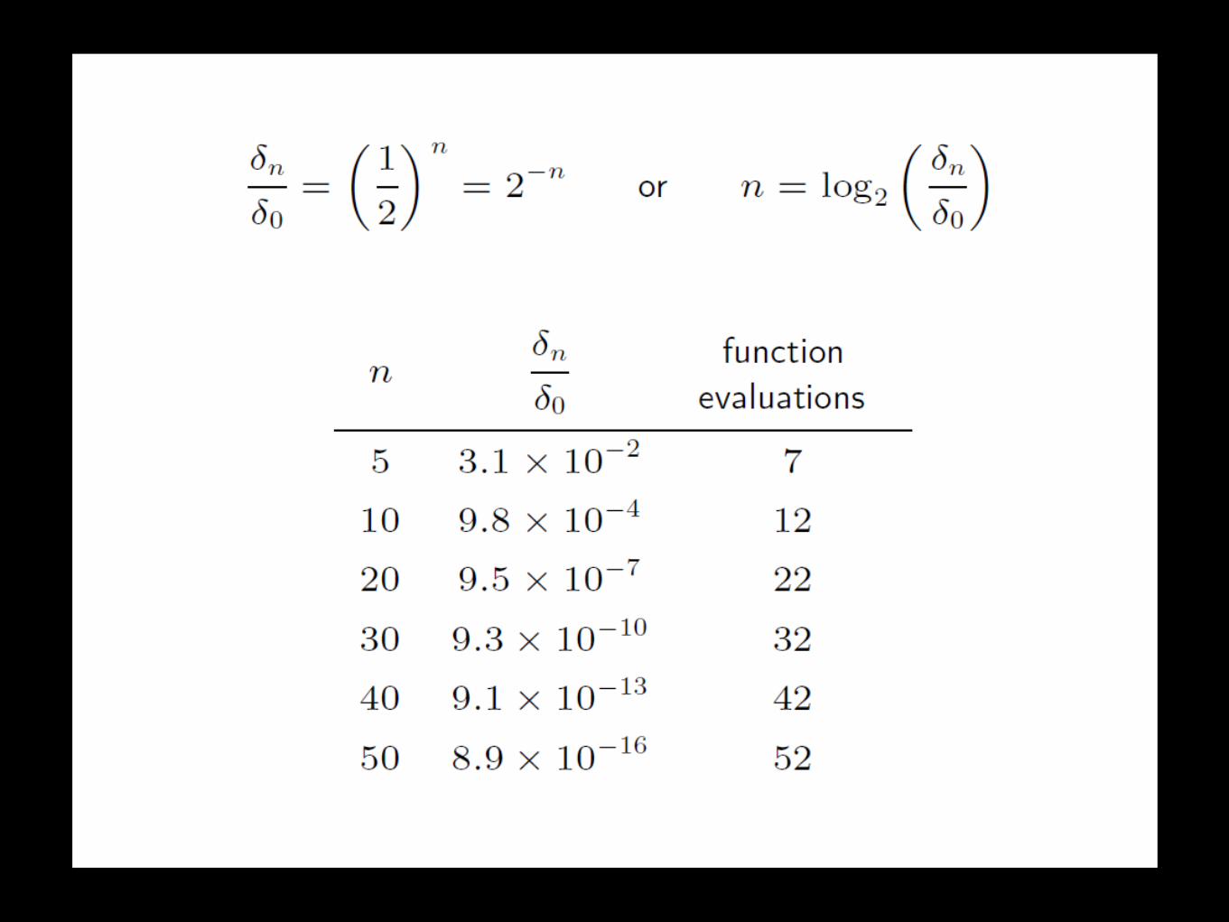
Convergence Rate of Bisection Method• The error after n iteration is smaller than |(b-a)/2n|.• Since the bracket size is reduced by a constant factor

at each step, the convergence rate (i.e., the reduction in the error) is said to be linear.

Bisection MethodIf we want, we can have the sequence of xk, which will be conveniently the sequence of xmid.

Convergence Rate of Fix-Point Method

• ds

Convergence of Newton’s Method

The quadratic convergence of Newton’s method comes with restrictions.

• Newton’s method is not guaranteed to converge unless |x0-ξ|≤ρ, where, in general, both ξ and ρ are not known.

• In other words, Newton’s method converges if the initial guess is close enough to the root, but neither the root nor a measure of “close enough” can be prescribed ahead of time.

• If f(x) has multiple roots (or root of multiplicity), f’(ξ)=0, the convergence of Newton’s method is only linear, not quadratic.

• Investigate the convergence behavior of f(x)=x2-1 and f(x)=x2-2x-1.

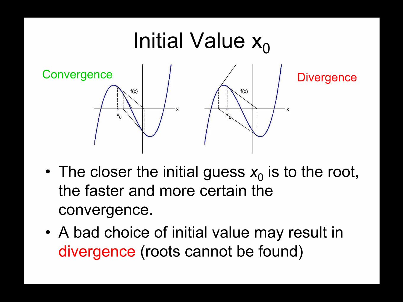
Initial Value x0

• The closer the initial guess x0 is to the root, the faster and more certain the convergence.

• A bad choice of initial value may result in divergence (roots cannot be found)

Convergence Divergence

System of Nonlinear Equations

• We now consider nonlinear equations in more than one dimension.

• The multidimensional case is much more difficult than the scalar case for a variety of reasons:– A much wider range of behavior is possible, so that a theoretical

analysis of the existence and number of solution is much more complex.

– It is not possible, in general, to guarantee convergence to the correction solution or to bracket the solution to produce an absolutely safe method.

– Computational overhead increases rapidly with the dimension of the problem.

• Many one-dimensional methods do not generalized directly to n dimensions.

• The most popular and powerful method that does generalize is Newton’s method.

Open Channel Hydraulics• Apply the principles of fluid mechanics to

surface-water flow in channels (e.g., rivers, streams, and canals).

• Why does the flow in rivers vary from deep and tranquil to shallow and torrential?

• What controls the depth of water in a river? • How are water depth and discharge in a

stream related?

Open Channel FlowDifference between open channel flow and pipe flow• The channel flow is only partially enclosed by a

solid boundary. • The upper "boundary" of an open channel flow,

between the water and the atmosphere, is called a free surface.

Start from simple case:flow to be steady and frictionless so that the Bernoulli

equation can be used.

Reach: A segment of a stream or river channel

Bernoulli’s Equation

In a very short reach, frictional losses and elevation change can be disregarded.

Convenient reference elevation. Sea level is often used.

Horizontal flow → no fluid acceleration in the vertical direction + steady state flow → total acceleration=0 → p=ρgd → p/ρg=d

→Specific energy (E [L]): the energy per unit weight of the flowing water relative to the stream bottom.

U

Measuring Flow in Natural Channels

• Current meter to measure river velocity and discharge.

Price current meter, 1882

Current meter or missile?

Nowadays

The current meter consists of a cup- or propeller-type rotor. The number of revolutions of the rotor in a given period (n) is directly proportional to the velocity (v) of the river: v=a+bn.

Propeller

Rectangular Sharp-crested Weir

Suppressed: rectangular sectionspans the full width of the channelWeir with end contraction: weir length less than the width of the channel

Notched Weirs

V-notch

If the elevation of the channel bottom remains constant, then because H is constant, E must also be constant.

Channel with a rectangular cross section

Specific discharge:

If E and qw are known, then h can be estimated.

Exercise

Solve h for E=0.75m and qw = 0.5 m2 s-1.

or

23 2( ) 0

2qf h h Ehg

� �

Find roots of f(x)=0.

The root Function

Specific Energy Diagram for a given qw

For E=0.75m and qw = 0.5 m2 s-1, there are three possible depths for the cubic equation relating E, qw, and h.The negative h3 has no physical meaning, and can be discarded. The other two depths are all possible, called alternative depths.

Bernoulli Equation + Continuity Equation Further work is needed!

The answer is gained by considering the relationship among:specific energy, specific discharge, and water depth.

Flow Over a Vertical Step

What will the surface do as the flow crosses the step: rise, fall, or remain unchanged?

z=0datum

Δz

Bernoulli’s Equation

the flow velocity and depth upstream of the step are known

h1h2?

constant

qw is known and constant, so we can create a specific energy diagram

• Locate E1 = 0.8 m• Estimate Δz = 0.1 m• Locate E2 = E1-Δz = 0.7 m• Find alternative solutions

h2 and h2’ (h1 > h2 > h2’) h1 → h2 → h0 → h2’

h1 → h2:Flow moves up Lose specific energyh2 → h0 → h2’:Gain specific energyFlow moves down Such a hump does not exist.

Along the same specific energy curve

h2 is the only solution physically meaningful

What is the relationship between h1 and h2 + Δz?

qw=U1h1=U2h2

h1>h2

U1<U2

the water surface drops and velocity increases as water flows over the step. This conclusion explains why canoeists are wary of sudden changes in stream elevation, as they often mean that large rocks are below.

What for a decrease step?

What if width changes?