Choosing roots of polynomials smoothly

Israel Journal of Mathematics 105 (1998), 203-233

CHOOSING ROOTS OF POLYNOMIALS SMOOTHLY

Dmitri Alekseevsky

Andreas Kriegl

Mark Losik

Peter W. Michor

Erwin Schrodinger International Instituteof Mathematical Physics, Wien, Austria

Abstract. We clarify the question whether for a smooth curve of polynomials one

can choose the roots smoothly and related questions. Applications to perturbationtheory of operators are given.

Table of contents

1. Introduction . . . . . . . . . . . . . . . . . . . . . . . . . . . . 1

2. Choosing differentiable square and cubic roots . . . . . . . . . . . . . 2

3. Choosing local roots of real polynomials smoothly . . . . . . . . . . . 7

4. Choosing global roots of polynomials differentiably . . . . . . . . . . . 11

5. The real analytic case . . . . . . . . . . . . . . . . . . . . . . . 14

6. Choosing roots of complex polynomials . . . . . . . . . . . . . . . . 16

7. Choosing eigenvalues and eigenvectors of matrices smoothly . . . . . . . 18

1. Introduction

We consider the following problem. Let

(1) P (t) = xn − a1(t)xn−1 + · · · + (−1)nan(t)

be a polynomial with all roots real, smoothly parameterized by t near 0 in R. Canwe find n smooth functions x1(t), . . . , xn(t) of the parameter t defined near 0, whichare the roots of P (t) for each t? We can reduce the problem to a1 = 0, replacingthe variable x by with the variable y = x− a1(t)/n. We will say that the curve (1)is smoothly solvable near t = 0 if such smooth roots xi(t) exist.

We describe an algorithm which in the smooth and in the holomorphic casesometimes allows to solve this problem. The main results are: If all roots are realthen they can always be chosen differentiable, but in general not C1 for degree

1991 Mathematics Subject Classification. 26C10.Key words and phrases. smooth roots of polynomials.Supported by ‘Fonds zur Forderung der wissenschaftlichen Forschung, Projekt P 10037 PHY’.

Typeset by AMS-TEX

1

2 D.V. ALEKSEEVSKY, A. KRIEGL, M. LOSIK, P.W. MICHOR

n ≥ 3; and in degree 2 they can be chosen twice differentiable but in general notC2. If they are arranged in increasing order, they depend continuously on thecoefficients of the polynomial, and if moreover no two of them meet of infinite orderin the parameter, then they can be chosen smoothly. We also apply these results toobtain a smooth 1-parameter perturbation theorem for selfadjoint operators withcompact resolvent under the condition, that no pair of eigenvalues meets of infiniteorder.

We thank C. Fefferman who found a mistake in a first version of 2.4, to M.and Th. Hoffmann-Ostenhof for their interest and hints, and to Jerry Kazdan forarranging [15].

2. Choosing differentiable square and cubic roots

2.1. Proposition. The case n = 2. Let P (t)(x) = x2 − f(t) for a function fdefined on an open interval, such that f(t) ≥ 0 for all t.

If f is smooth and is nowhere flat of infinite order, then smooth solutions x exist.If f is C2 then C1-solutions exist.If f is C4 then twice differentiable solutions exist.

Proof. Suppose that f is smooth. If f(t0) > 0 then we have obvious local smooth

solutions ±√

f(t). If f(t0) = 0 we have to find a smooth function x such thatf = x2, a smooth square root of f . If f is not flat at t0 then the first nonzeroderivative at t0 has even order 2m and is positive, and f(t) = (t − t0)

2mf2m(t),

where f2m(t) :=∫ 1

0(1−r)2m−1

(2m−1)! f (2m)(t0 + r(t − t0)) dr gives a smooth function and

f2m(t0) = 1(2m)!f

(2m)(t0) > 0. Then x(t) := (t − t0)m

√

f2m(t) is a local smooth

solution. One can piece together these local solutions, changing sign at all pointswhere the first non-vanishing derivative of f is of order 2m with m odd. Thesepoints are discrete.

Let us consider now a function f ≥ 0 of class C2. We claim that then x2 = f(t)admits a C1-root x(t), globally in t. We consider a fixed t0. If f(t0) > 0 then there

is locally even a C2-solution x±(t) = ±√

f(t). If f(t0) = 0 then f(t) = (t− t0)2h(t)

where h ≥ 0 is continuous and C2 off t0 with h(t0) = 12f ′′(t0). If h(t0) > 0 then

x±(t) = ±(t − t0)√

h(t) is C2 off t0, and

x′±(t0) = lim

t→t0

x±(t) − x±(t0)

t − t0= lim

t→t0±

√

h(t) = ±√

h(t0) = ±√

12f ′′(t0).

If h(t0) = 0 then we choose x±(t0) = 0, and any choice of the roots is thendifferentiable at t0 with derivative 0, by the same calculation.

One can piece together these local solutions: At zeros t of f where f ′′(t) > 0we have to pass through 0, but where f ′′(t) = 0 the choice of the root does notmatter. The set {t : f(t) = f ′′(t) = 0} is closed, so its complement is a union ofopen intervals. Choose a point in each of these intervals where f(t) > 0 and startthere with the positive root, changing signs at points where f(t) = 0 6= f ′′(t): thesepoints do not accumulate in the intervals. Then we get a differentiable choice ofa root x(t) on each of this open intervals which extends to a global differentiableroot which is 0 on {t : f(t) = f ′′(t) = 0}.

CHOOSING ROOTS OF POLYNOMIALS SMOOTHLY 3

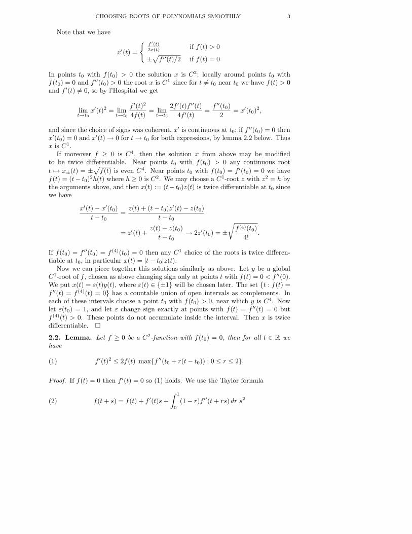
Note that we have

x′(t) =

{

f ′(t)2x(t) if f(t) > 0

±√

f ′′(t)/2 if f(t) = 0

In points t0 with f(t0) > 0 the solution x is C2; locally around points t0 withf(t0) = 0 and f ′′(t0) > 0 the root x is C1 since for t 6= t0 near t0 we have f(t) > 0and f ′(t) 6= 0, so by l’Hospital we get

limt→t0

x′(t)2 = limt→t0

f ′(t)2

4f(t)= lim

t→t0

2f ′(t)f ′′(t)

4f ′(t)=

f ′′(t0)

2= x′(t0)

2,

and since the choice of signs was coherent, x′ is continuous at t0; if f ′′(t0) = 0 thenx′(t0) = 0 and x′(t) → 0 for t → t0 for both expressions, by lemma 2.2 below. Thusx is C1.

If moreover f ≥ 0 is C4, then the solution x from above may be modifiedto be twice differentiable. Near points t0 with f(t0) > 0 any continuous root

t 7→ x±(t) = ±√

f(t) is even C4. Near points t0 with f(t0) = f ′(t0) = 0 we havef(t) = (t− t0)

2h(t) where h ≥ 0 is C2. We may choose a C1-root z with z2 = h bythe arguments above, and then x(t) := (t− t0)z(t) is twice differentiable at t0 sincewe have

x′(t) − x′(t0)

t − t0=

z(t) + (t − t0)z′(t) − z(t0)

t − t0

= z′(t) +z(t) − z(t0)

t − t0→ 2z′(t0) = ±

√

f (4)(t0)

4!.

If f(t0) = f ′′(t0) = f (4)(t0) = 0 then any C1 choice of the roots is twice differen-tiable at t0, in particular x(t) = |t − t0|z(t).

Now we can piece together this solutions similarly as above. Let y be a globalC1-root of f , chosen as above changing sign only at points t with f(t) = 0 < f ′′(0).We put x(t) = ε(t)y(t), where ε(t) ∈ {±1} will be chosen later. The set {t : f(t) =f ′′(t) = f (4)(t) = 0} has a countable union of open intervals as complements. Ineach of these intervals choose a point t0 with f(t0) > 0, near which y is C4. Nowlet ε(t0) = 1, and let ε change sign exactly at points with f(t) = f ′′(t) = 0 butf (4)(t) > 0. These points do not accumulate inside the interval. Then x is twicedifferentiable. ¤

2.2. Lemma. Let f ≥ 0 be a C2-function with f(t0) = 0, then for all t ∈ R wehave

(1) f ′(t)2 ≤ 2f(t) max{f ′′(t0 + r(t − t0)) : 0 ≤ r ≤ 2}.

Proof. If f(t) = 0 then f ′(t) = 0 so (1) holds. We use the Taylor formula

(2) f(t + s) = f(t) + f ′(t)s +

∫ 1

0

(1 − r)f ′′(t + rs) dr s2


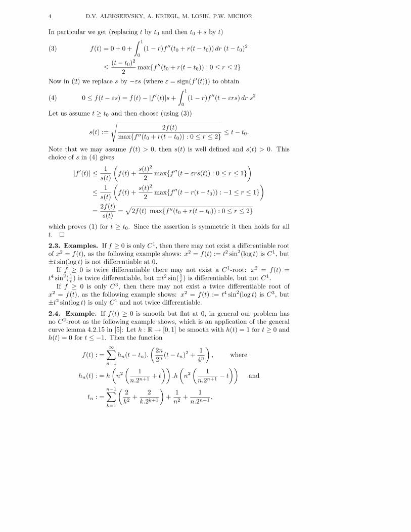
In particular we get (replacing t by t0 and then t0 + s by t)

f(t) = 0 + 0 +

∫ 1

0

(1 − r)f ′′(t0 + r(t − t0)) dr (t − t0)2(3)

≤ (t − t0)2

2max{f ′′(t0 + r(t − t0)) : 0 ≤ r ≤ 2}

Now in (2) we replace s by −εs (where ε = sign(f ′(t))) to obtain

(4) 0 ≤ f(t − εs) = f(t) − |f ′(t)|s +

∫ 1

0

(1 − r)f ′′(t − εrs) dr s2

Let us assume t ≥ t0 and then choose (using (3))

s(t) :=

√

2f(t)

max{f ′′(t0 + r(t − t0)) : 0 ≤ r ≤ 2} ≤ t − t0.

Note that we may assume f(t) > 0, then s(t) is well defined and s(t) > 0. Thischoice of s in (4) gives

|f ′(t)| ≤ 1

s(t)

(

f(t) +s(t)2

2max{f ′′(t − εrs(t)) : 0 ≤ r ≤ 1}

)

≤ 1

s(t)

(

f(t) +s(t)2

2max{f ′′(t − r(t − t0)) : −1 ≤ r ≤ 1}

)

=2f(t)

s(t)=

√

2f(t) max{f ′′(t0 + r(t − t0)) : 0 ≤ r ≤ 2}

which proves (1) for t ≥ t0. Since the assertion is symmetric it then holds for allt. ¤

2.3. Examples. If f ≥ 0 is only C1, then there may not exist a differentiable rootof x2 = f(t), as the following example shows: x2 = f(t) := t2 sin2(log t) is C1, but±t sin(log t) is not differentiable at 0.

If f ≥ 0 is twice differentiable there may not exist a C1-root: x2 = f(t) =t4 sin2( 1

t ) is twice differentiable, but ±t2 sin(1t ) is differentiable, but not C1.

If f ≥ 0 is only C3, then there may not exist a twice differentiable root ofx2 = f(t), as the following example shows: x2 = f(t) := t4 sin2(log t) is C3, but±t2 sin(log t) is only C1 and not twice differentiable.

2.4. Example. If f(t) ≥ 0 is smooth but flat at 0, in general our problem hasno C2-root as the following example shows, which is an application of the generalcurve lemma 4.2.15 in [5]: Let h : R → [0, 1] be smooth with h(t) = 1 for t ≥ 0 andh(t) = 0 for t ≤ −1. Then the function

f(t) : =

∞∑

n=1

hn(t − tn).

(

2n

2n(t − tn)2 +

1

4n

)

, where

hn(t) : = h

(

n2

(

1

n.2n+1+ t

))

.h

(

n2

(

1

n.2n+1− t

))

and

tn : =n−1∑

k=1

(

2

k2+

2

k.2k+1

)

+1

n2+

1

n.2n+1,


is ≥ 0 and is smooth: the sum consists of at most one summand for each t, andthe derivatives of the summands converge uniformly to 0: Note that hn(t) = 1 for|t| ≤ 1

n.2n+1 and hn(t) = 0 for |t| ≥ 1n.2n+1 + 1

n2 hence hn(t − tn) 6= 0 only for

rn < t < rn+1, where rn :=∑n−1

k=1

(

2k2 + 2

k.2k+1

)

. Let cn(s) := 2n2n s2 + 1

4n ≥ 0 and

Hi := sup{|h(i)(t)| : t ∈ R}. Then

n2 sup{|(hn · cn)(k)(t)| : t ∈ R} = n2 sup{|(hn · cn)(k)(t)| : |t| ≤ 1

n.2n+1+

1

n2}

≤ n2k

∑

i=0

(

k

i

)

n2iHi sup{|c(k−i)n (t)| : |t| ≤ 1

n.2n+1+

1

n2}

≤( k

∑

i=0

(

k

i

)

n2i+2Hi

)

sup{|c(j)n (t)| : |t| ≤ 2, j ≤ k}

and since cn is rapidly decreasing in C∞(R, R) (i.e. {p(n) cn : n ∈ N} is bounded inC∞(R, R) for each polynomial p) the right side of the inequality above is boundedwith respect to n ∈ N and hence the series

∑

n hn( −tn)cn( −tn) convergesuniformly in each derivative, and thus represents an element of f ∈ C∞(R, R).Moreover we have

f(tn) =1

4n, f ′(tn) = 0, f ′′(tn) =

2n

2n−1.

Let us assume that f(t) = g(t)2 for t near supn tn < ∞, where g is twice differen-tiable. Then

f ′ = 2gg′

f ′′ = 2gg′′ + 2(g′)2

2ff ′′ = 4g3g′′ + (f ′)2

2f(tn)f ′′(tn) = 4g(tn)3g′′(tn) + f ′(tn)2

thus g′′(tn) = ±2n, so g cannot be C2, and g′ cannot satisfy a local Lipschitzcondition near lim tn. Another similar example can be found in 7.4 below.

According to [15], some results of this section are contained in Frank Warnersdissertation (around 1963, unpublished): Non-negative smooth functions have C1

square roots whose second derivatives exist everywhere. If all zeros are of finiteorder there are smooth square roots. However, there are examples not possessinga C2 square root. Here is one:

f(t) = sin2(1/t)e−1/t + e−2/t for t > 0, f(t) = 0 for t ≤ 0.

This is a sum of two non-negative C∞ functions each of which has a C∞ squareroot. But the second derivative of the square root of f is not continuous at theorigin.

In [6] Glaeser proved that a non-negative C2-function on an open subset of Rn

which vanishes of second order has a C1 positive square root. A smooth functionf ≥ 0 is constructed which is flat at 0 such that the positive square root is not C2.In [4] Dieudonne gave shorter proofs of Glaeser’s results.


2.5. Example. The case n ≥ 3. We will construct a polynomial

P (t) = x3 + a2(t)x − a3(t)

with smooth coefficients a2, a3 with all roots real which does not admit C1-roots.Multiplying with other polynomials one then gets polynomials of all orders n ≥ 3which do not admit C1-roots.

Suppose that P admits C1-roots x1, x2, x3. Then we have

0 = x1 + x2 + x3

a2 = x1x2 + x2x3 + x3x1

a3 = x1x2x3

0 = x1 + x2 + x3

a2 = x1x2 + x1x2 + x2x3 + x2x3 + x3x1 + x3x1

a3 = x1x2x3 + x1x2x3 + x1x2x3

We solve the linear system formed by the last three equations and get

x1 =a3 − a2x1

(x2 − x1)(x3 − x1)

x2 =a3 − a2x2

(x3 − x2)(x1 − x2)

x3 =a3 − a2x3

(x1 − x3)(x2 − x3).

We consider the continuous function

b3 := x1x2x3 =a33 + a2

2a3a2 − a32a3

4a32 + 27a2

3

.

For smooth functions f and ε with ε2 ≤ 1 we let

u : = −12a2 := f2

v : = 108a3 := εf3.

then all roots of P are real since a2 ≤ 0 and 432(4a32+27a2

3) = v2−u3 = f6(ε2−1) ≤0. We get then

11664b3 =4v3 − 27uu2v + 27u3v

v2 − u3

= 4f3ε3 + 9f2f ε2ε + 27ff2ε(ε2 − 1) + 27f3ε(ε2 − 3)

ε2 − 1.

Now we choose

f(t) : =∞∑

n=1

hn(t − tn).( n

2n(t − tn)

)

,

ε(t) : = 1 −∞∑

n=1

hn(t − tn).1

8n,


where hn and tn are as in the beginning of 2.4. Then f(tn) = 0, f(tn) = n2n , and

ε(tn) = 18n , hence

108b3(tn) =f(tn)3ε(tn)(ε(tn)2 − 3)

ε(tn)2 − 1∼ n3 → ∞

is unbounded on the convergent sequence tn. So the roots cannot be chosen locallyLipschitz, thus not C1.

3. Choosing local roots of real polynomials smoothly

3.1. Preliminaries. We recall some known facts on polynomials with real coeffi-cients. Let

P (x) = xn − a1xn−1 + · · · + (−1)nan

be a polynomial with real coefficients a1, . . . , an and roots x1, . . . , xn ∈ C. Itis known that ai = σi(x1, . . . , xn), where σi (i = 1, . . . , n) are the elementarysymmetric functions in n variables:

σi(x1, . . . , xn) =∑

1≤j1<···<ji≤n

xj1 . . . xji

Denote by si the Newton polynomials∑n

j=1 xij which are related to the elementary

symmetric function by

(1) sk − sk−1σ1 + sk−2σ2 + · · · + (−1)k−1s1σk−1 + (−1)kkσk = 0 (k ≤ n)

The corresponding mappings are related by a polynomial diffeomorphism ψn, givenby (1):

σn : = (σ1, . . . , σn) : Rn → R

n

sn : = (s1, . . . , sn) : Rn → R

n

sn : = ψn ◦ σn

Note that the Jacobian (the determinant of the derivative) of sn is n! times theVandermonde determinant: det(dsn(x)) = n!

∏

i>j(xi−xj) =: n! Van(x), and even

the derivative itself d(sn)(x) equals the Vandermonde matrix up to factors i in thei-th row. We also have det(d(ψn)(x)) = (−1)n(n+3)/2n! = (−1)n(n−1)/2n!, andconsequently det(dσn(x)) =

∏

i>j(xj − xi). We consider the so-called Bezoutiant

B :=

s0 s1 . . . sn−1

s1 s2 . . . sn...

......

sn−1 sn . . . s2n−2

.

Let Bk be the minor formed by the first k rows and columns of B. From

Bk(x) =

1 1 . . . 1x1 x2 . . . xn...

......

xk−11 xk−1

2 . . . xk−1n

·

1 x1 . . . xk−11

1 x2 . . . xk−12

......

...1 xn . . . xk−1

n


it follows that

(2) ∆k(x) := det(Bk(x)) =∑

i1<i2<···<ik

(xi1 −xi2)2 . . . (xi1 −xik

)2 . . . (xik−1−xik

)2,

since for n × k-matrices A one has det(AA⊤) =∑

i1<···<ikdet(Ai1,...,ik

)2, whereAi1,...,ik

is the minor of A with indicated rows. Since the ∆k are symmetric we

have ∆k = ∆k ◦ σn for unique polynomials ∆k and similarly we shall use B.

3.2. Theorem. (Sylvester’s version of Sturm’s theorem, see [14], [10]) The roots

of P are all real if and only if the symmetric (n × n) matrix B(P ) is positive

semidefinite; then ∆k(P ) := ∆k(a1, . . . , an) ≥ 0 for 1 ≤ k ≤ n. The rank of Bequals the number of distinct roots of P and its signature equals the number ofdistinct real roots.

3.3. Proposition. Let now P be a smooth curve of polynomials

P (t)(x) = xn − a1(t)xn−1 + · · · + (−1)nan(t)

with all roots real, and distinct for t = 0. Then P is smoothly solvable near 0.This is also true in the real analytic case and for higher dimensional parameters,

and in the holomorphic case for complex roots.

Proof. The derivative ddxP (0)(x) does not vanish at any root, since they are dis-

tinct. Thus by the implicit function theorem we have local smooth solutions x(t)of P (t, x) = P (t)(x) = 0. ¤

3.4. Splitting Lemma. Let P0 be a polynomial

P0(x) = xn − a1xn−1 + · · · + (−1)nan.

If P0 = P1 ·P2, where P1 and P2 are polynomials with no common root. Then for Pnear P0 we have P = P1(P )P2(P ) for real analytic mappings of monic polynomialsP 7→ P1(P ) and P 7→ P2(P ), defined for P near P0, with the given initial values.

Proof. Let the polynomial P0 be represented as the product

P0 = P1.P2 = (xp − b1xp−1 + · · · + (−1)pbp)(x

q − c1xq−1 + · · · + (−1)qcq),

let xi for i = 1, . . . , n be the roots of P0, ordered in such a way that for i = 1, . . . , pwe get the roots of P1, and for i = p + 1, . . . , p + q = n we get those of P2. Then(a1, . . . , an) = φp,q(b1, . . . , bp, c1, . . . , cq) for a polynomial mapping φp,q and we get

σn = φp,q ◦ (σp × σq),

det(dσn) = det(dφp,q(b, c)) det(dσp) det(dσq).

From 3.1 we conclude∏

1≤i<j≤n

(xi − xj) = det(dφp,q(b, c))∏

1≤i<j≤p

(xi − xj)∏

p+1≤i<j≤n

(xi − xj)

which in turn implies

det(dφp,q(b, c)) =∏

1≤i≤p<j≤n

(xi − xj) 6= 0

so that φp,q is a real analytic diffeomorphism near (b, c). ¤


3.5. For a continuous function f defined near 0 in R let the multiplicity or orderof flatness m(f) at 0 be the supremum of all integer p such that f(t) = tpg(t)near 0 for a continuous function g. If f is Cn and m(f) < n then f(t) = tm(f)g(t)where now g is Cn−m(f) and g(0) 6= 0. If f is a continuous function on the spaceof polynomials, then for a fixed continuous curve P of polynomials we will denoteby m(f) the multiplicity at 0 of t 7→ f(P (t)).

The splitting lemma 3.4 shows that for the problem of smooth solvability it isenough to assume that all roots of P (0) are equal.

Proposition. Suppose that the smooth curve of polynomials

P (t)(x) = xn + a2(t)xn−2 − · · · + (−1)nan(t)

is smoothly solvable with smooth roots t 7→ xi(t), and that all roots of P (0) areequal. Then for (k = 2, . . . , n)

m(∆k) ≥ k(k − 1) min1≤i≤n

m(xi)

m(ak) ≥ k min1≤i≤n

m(xi)

This result also holds in the real analytic case and in the smooth case.

Proof. This follows from 3.1.(2) for ∆k, and from ak(t) = σk(x1(t), . . . , xn(t)). ¤

3.6. Lemma. Let P be a polynomial of degree n with all roots real. If a1 = a2 = 0then all roots of P are equal to zero.

Proof. From 3.1.(1) we have∑

x2i = s2(x) = σ2

1(x) − 2σ2(x) = a21 − 2a2 = 0. ¤

3.7. Multiplicity lemma. Consider a smooth curve of polynomials

P (t)(x) = xn + a2(t)xn−2 − · · · + (−1)nan(t)

with all roots real. Then, for integers r, the following conditions are equivalent:

(1) m(ak) ≥ kr for all 2 ≤ k ≤ n.

(2) m(∆k) ≥ k(k − 1)r for all 2 ≤ k ≤ n.(3) m(a2) ≥ 2r.

Proof. We only have to treat r > 0.(1) implies (2): From 3.1.(1) we have m(sk) ≥ rk, and from the definition of

∆k = det(Bk) we get (2).

(2) implies (3) since ∆2 = −2na2.(3) implies (1): From a2(0) = 0 and lemma 3.6 it follows that all roots of the

polynomial P (0) are equal to zero and, then, a3(0) = · · · = an(0) = 0. There-fore, m(a3), . . . ,m(an) ≥ 1. Under these conditions, we have a2(t) = t2ra2,2r(t)and ak(t) = tmkak,mk

(t) for k = 3, . . . , n, where the mk are positive integers anda2,2r, a3,m3

, . . . , an,mnare smooth functions, and where we may assume that either

mk = m(ak) < ∞ or mk ≥ kr.Suppose now indirectly that for some k > 2 we have mk = m(ak) < kr. Then

we put

m := min(r,m3

3, . . . ,

mn

n) < r.


We consider the following continuous curve of polynomials for t ≥ 0:

Pm(t)(x) := xn + a2,2r(t)t2r−2mxn−2

− a3,m3(t)tm3−3mxn−3 + · · · + (−1)nan,mn

(t)tmn−nm.

If x1, . . . , xn are the real roots of P (t) then t−mx1, . . . , t−mxn are the roots of Pm(t),

for t > 0. So for t > 0, Pm(t) is a family of polynomials with all roots real. Sinceby theorem 3.2 the set of polynomials with all roots real is closed, Pm(0) is also apolynomial with all roots real.

By lemma 3.6 all roots of the polynomial Pm(0) are equal to zero, and forthose k with mk = km we have ak,mk

(0) = 0 and, therefore, m(ak) > mk, acontradiction. ¤

3.8. Algorithm. Consider a smooth curve of polynomials

P (t)(x) = xn − a1(t)xn−1 + a2(t)x

n−2 − · · · + (−1)nan(t)

with all roots real. The algorithm has the following steps:

(1) If all roots of P (0) are pairwise different, P is smoothly solvable for t near0 by 3.3.

(2) If there are distinct roots at t = 0 we put them into two subsets which splitsP (t) = P1(t).P2(t) by the splitting lemma 3.4. We then feed Pi(t) (whichhave lower degree) into the algorithm.

(3) All roots of P (0) are equal. We first reduce P (t) to the case a1(t) = 0 byreplacing the variable x by y = x − a1(t)/n. Then all roots are equal to 0so m(a2) > 0.

(3a) If m(a2) is finite then it is even since ∆2 = −2na2 ≥ 0, m(a2) = 2r and bythe multiplicity lemma 3.7 ai(t) = ai,ir(t)t

ir (i = 2, . . . , n) for smooth ai,ir.Consider the following smooth curve of polynomials

Pr(t)(x) = xn + a2,2r(t)xn−2 − a3,3r(t)x

n−3 · · · + (−1)nan,nr(t).

If Pr(t) is smoothly solvable and xk(t) are its smooth roots, then xk(t)tr arethe roots of P (t) and the original curve P is smoothly solvable too. Sincea2,2m(0) 6= 0, not all roots of Pr(0) are equal and we may feed Pr into step2 of the algorithm.

(3b) If m(a2) is infinite and a2 = 0, then all roots are 0 by 3.6 and thus thepolynomial is solvable.

(3c) But if m(a2) is infinite and a2 6= 0, then by the multiplicity lemma 3.7 allm(ai) for 2 ≤ i ≤ n are infinite. In this case we keep P (t) as factor of theoriginal curve of polynomials with all coefficients infinitely flat at t = 0 afterforcing a1 = 0. This means that all roots of P (t) meet of infinite order offlatness (see 3.5) at t = 0 for any choice of the roots. This can be seen asfollows: If x(t) is any root of P (t) then y(t) := x(t)/tr is a root of Pr(t),hence by 4.1 bounded, so x(t) = tr−1.ty(t) and t 7→ ty(t) is continuous att = 0.


This algorithm produces a splitting of the original polynomial

P (t) = P (∞)(t)P (s)(t)

where P (∞) has the property that each root meets another one of infinite order att = 0, and where P (s)(t) is smoothly solvable, and no two roots meet of infiniteorder at t = 0, if they are not equal. Any two choices of smooth roots of P (s) differby a permutation.

The factor P (∞) may or may not be smoothly solvable. For a flat function f ≥ 0consider:

x4 − (f(t) + t2)x2 + t2f(t) = (x2 − f(t)).(x − t)(x + t).

Here the algorithm produces this factorization. For f(t) = g(t)2 the polynomial issmoothly solvable. For the smooth function f from 2.4 it is not smoothly solvable.

4. Choosing global roots of polynomials differentiably

4.1. Lemma. For a polynomial

P (x) = xn − a1(P )xn−1 + · · · + (−1)nan(P )

with all roots real, i.e. ∆k(P ) = ∆k(a1, . . . , an) ≥ 0 for 1 ≤ k ≤ n, let

x1(P ) ≤ x2(P ) ≤ · · · ≤ xn(P )

be the roots, increasingly ordered.Then all xi : σn(Rn) → R are continuous.

Proof. We show first that x1 is continuous. Let P0 ∈ σn(Rn) be arbitrary. We haveto show that for every ε > 0 there exists some δ > 0 such that for all |P − P0| < δthere is a root x(P ) of P with x(P ) < x1(P0)+ε and for all roots x(P ) of P we havex(P ) > x1(P0) − ε. Without loss of generality we may assume that x1(P0) = 0.

We use induction on the degree n of P . By the splitting lemma 3.4 for the C0-casewe may factorize P as P1(P ) ·P2(P ), where P1(P0) has all roots equal to x1 = 0 andP2(P0) has all roots greater than 0 and both polynomials have coefficients whichdepend real analytically on P . The degree of P2(P ) is now smaller than n, so byinduction the roots of P2(P ) are continuous and thus larger than x1(P0) − ε for Pnear P0.

Since 0 was the smallest root of P0 we have to show that for all ε > 0 there existsa δ > 0 such that for |P − P0| < δ any root x of P1(P ) satisfies |x| < ε. Supposethere is a root x with |x| ≥ ε. Then we get as follows a contradiction, where n1 isthe degree of P1. From

−xn1 =

n1∑

k=1

(−1)kak(P1)xn1−k

we have

ε ≤ |x| =∣

∣

∣

n1∑

k=1

(−1)kak(P1)x1−k

∣

∣

∣≤

n1∑

k=1

|ak(P1)| |x|1−k <

n1∑

k=1

εk

n1ε1−k = ε,


provided that n1|ak(P1)| < εk, which is true for P1 near P0, since ak(P0) = 0. Thusx1 is continuous.

Now we factorize P = (x − x1(P )) · P2(P ), where P2(P ) has roots x2(P ) ≤· · · ≤ xn(P ). By Horner’s algorithm (an = bn−1x1, an−1 = bn−1 + bn−2x1, . . . ,a2 = b2 + b1x1, a1 = b1 + x1) the coefficients bk of P2(P ) are again continuous andso we may proceed by induction on the degree of P . Thus the claim is proved. ¤

4.2. Theorem. Consider a smooth curve of polynomials

P (t)(x) = xn + a2(t)xn−2 − · · · + (−1)nan(t)

with all roots real, for t ∈ R. Let one of the two following equivalent conditions besatisfied:

(1) If two of the increasingly ordered continuous roots meet of infinite ordersomewhere then they are equal everywhere.

(2) Let k be maximal with the property that ∆k(P ) does not vanish identically

for all t. Then ∆k(P ) vanishes nowhere of infinite order.

Then the roots of P can be chosen smoothly, and any two choices differ by apermutation of the roots.

Proof. The local situation. We claim that for any t0, without loss t0 = 0, thefollowing conditions are equivalent:

(1) If two of the increasingly ordered continuous roots meet of infinite order att = 0 then their germs at t = 0 are equal.

(2) Let k be maximal with the property that the germ at t = 0 of ∆k(P ) is not

0. Then ∆k(P ) is not infinitely flat at t = 0.(3) The algorithm 3.8 never leads to step (3c).

(3) =⇒ (1). Suppose indirectly that two nonequal of the increasingly orderedcontinuous roots meet of infinite order at t = 0. Then in each application of step (2)these two roots stay with the same factor. After any application of step (3a) thesetwo roots lead to nonequal roots of the modified polynomial which still meet ofinfinite order at t = 0. They never end up in a facter leading to step (3b) orstep (1). So they end up in a factor leading to step (3c).(1) =⇒ (2). Let x1(t) ≤ · · · ≤ xn(t) be the continuous roots of P (t). From 3.1, (2)we have

(4) ∆k(P (t)) =∑

i1<i2<···<ik

(xi1 − xi2)2 . . . (xi1 − xin

)2 . . . (xik−1− xik

)2.

The germ of ∆k(P ) is not 0, so the germ of one summand is not 0. If ∆k(P ) wereinfinitely flat at t = 0, then each summand is infinitely flat, so there are two rootsamong the xi which meet of infinite order, thus by assumption their germs areequal, so this summand vanishes.(2) =⇒ (3). Since the leading ∆k(P ) vanishes only of finite order at zero, P hasexactly k different roots off 0. Suppose indirectly that the algorithm 3.8 leads tostep (3c), then P = P (∞)P (s) for a nontrivial polynomial P (∞). Let x1(t) ≤ · · · ≤xp(t) be the roots of P (∞)(t) and xp+1(t) ≤ · · · ≤ xn(t) those of P (s). We know


that each xi meets some xj of infinite order and does not meet any xl of infinite

order, for i, j ≤ p < l. Let k(∞) > 2 and k(s) be the number of generically differentroots of P (∞) and P (s), respectively. Then k = k(∞) + k(s), and an inspection ofthe formula for ∆k(P ) above leads to the fact that it must vanish of infinite orderat 0, since the only non-vanishing summands involve exactly k(∞) many genericallydifferent roots from P (∞).

The global situation. From the first part of the proof we see that the algorithm3.8 allows to choose the roots smoothly in a neighborhood of each point t ∈ R, andthat any two choices differ by a (constant) permutation of the roots. Thus we mayglue the local solutions to a global solution. ¤

4.3. Theorem. Consider a curve of polynomials

P (t)(x) = xn − a1(t)xn−1 + · · · + (−1)nan(t), t ∈ R,

with all roots real, where all ai are of class Cn. Then there is a differentiable curvex = (x1, . . . , xn) : R → R

n whose coefficients parameterize the roots.

That this result cannot be improved to C2-roots is shown already in 2.4, andnot to C1 for n ≥ 3 is shown in 2.5.

Proof. First we note that the multiplicity lemma 3.7 remains true in the Cn-casefor r = 1 in the following sense, with the same proof:If a1 = 0 then the following two conditions are equivalent

(1) ak(t) = tkak,k(t) for a continuous function ak,k, for 2 ≤ k ≤ n.

(2) a2(t) = t2a2,2(t) for a continuous function a2,2.

In order to prove the theorem itself we follow one step of the algorithm. Firstwe replace x by x + 1

na1(t), or assume without loss that a1 = 0. Then we choose afixed t, say t = 0.

If a2(0) = 0 then it vanishes of second order at 0: if it vanishes only of first

order then ∆2(P (t)) = −2na2(t) would change sign at t = 0, contrary to theassumption that all roots of P (t) are real, by 3.2. Thus a2(t) = t2a2,2(t), so bythe variant of the multiplicity lemma 3.7 described above we have ak(t) = tkak,k(t)for continuous functions ak,k, for 2 ≤ k ≤ n. We consider the following continuouscurve of polynomials

P1(t)(x) = xn + a2,2(t)xn−2 − a3,3(t)x

n−3 · · · + (−1)nan,n(t).

with continuous roots z1(t) ≤ · · · ≤ zn(t), by 4.1. Then xk(t) = zk(t)t are dif-ferentiable at 0, and are all roots of P , but note that xk(t) = yk(t) for t ≥ 0,but xk(t) = yn−k(t) for t ≤ 0, where y1(t) ≤ · · · ≤ yn(t) are the ordered roots ofP (t). This gives us one choice of differentiable roots near t = 0. Any choice is thengiven by this choice and applying afterwards any permutation of the set {1, . . . , n}keeping invariant the function k 7→ zk(0).

If a2(0) 6= 0 then by the splitting lemma 3.4 for the Cn-case we may factorP (t) = P1(t) . . . Pk(t) where the Pi(t) have again Cn-coefficients and where eachPi(0) has all roots equal to ci, and where the ci are distinct. By the arguments


above the roots of each Pi can be arranged differentiably, thus P has differentiableroots yk(t).

But note that we have to apply a permutation on one side of 0 to the originalroots, in the following case: Two roots xk and xl meet at zero with xk(t)− xl(t) =tckl(t) with ckl(0) 6= 0 (we say that they meet slowly). We may apply to this choicean arbitrary permutation of any two roots which meet with ckl(0) = 0 (i.e. at leastof second order), and we get thus any differentiable choice near t = 0.

Now we show that we choose the roots differentiable on the whole domain R.We start with with the ordered continuous roots y1(t) ≤ · · · ≤ yn(t). Then we put

xk(t) = yσ(t)(k)(t)

where the permutation σ(t) is given by

σ(t) = (1, 2)ε1,2(t) . . . (1, n)ε1,n(t)(2, 3)ε2,3(t) . . . (n − 1, n)εn−1,n(t)

and where εi,j(t) ∈ {0, 1} will be specified as follows: On the closed set Si,j of all twhere yi(t) and yj(t) meet of order at least 2 any choice is good. The complementof Si,j is an at most countable union of open intervals, and in each interval wechoose a point where we put εi,j = 0. Going right (and left) from this point wechange εi,j in each point where yi and yj meet slowly. These points accumulateonly in Si,j . ¤

5. The real analytic case

5.1. Theorem. Let P be a real analytic curve of polynomials

P (t)(x) = xn − a1(t)xn−1 + · · · + (−1)nan(t), t ∈ R,

with all roots real.Then P is real analytically solvable, globally on R. All solutions differ by per-

mutations.

By a real analytic curve of polynomials we mean that all ai(t) are real analyticin t (but see also [8]), and real analytically solvable means that we may find xi(t)for i = 1, . . . , n which are real analytic in t and are roots of P (t) for all t. Thelocal existence part of this theorem is due to Rellich [11], Hilfssatz 2, his proof usesPuiseux-expansions. Our proof is different and more elementary.

Proof. We first show that P is locally real analytically solvable, near each pointt0 ∈ R. It suffices to consider t0 = 0. Using the transformation in the introductionwe first assume that a1(t) = 0 for all t. We use induction on the degree n. If n = 1the theorem holds. For n > 1 we consider several cases:

The case a2(0) 6= 0. Here not all roots of P (0) are equal and zero, so by thesplitting lemma 3.4 we may factor P (t) = P1(t).P2(t) for real analytic curves ofpolynomials of positive degree, which have both all roots real, and we have reducedthe problem to lower degree.

The case a2(0) = 0. If a2(t) = 0 for all t, then by 3.6 all roots of P (t) are 0,and we are done. Otherwise 1 ≤ m(a2) < ∞ for the multiplicity of a2 at 0, and


by 3.6 all roots of P (0) are 0. If m(a2) > 0 is odd, then ∆2(P )(t) = −2na2(t)changes sign at t = 0, so by 3.2 not all roots of P (t) are real for t on one side of 0.This contradicts the assumption, so m(a2) = 2r is even. Then by the multiplicitylemma 3.7 we have ai(t) = ai,ir(t)t

ir (i = 2, . . . , n) for real analytic ai,ir, and wemay consider the following real analytic curve of polynomials


n−3 · · · + (−1)nan,nr(t),

with all roots real. If Pr(t) is real analytically solvable and xk(t) are its real analyticroots, then xk(t)tr are the roots of P (t) and the original curve P is real analyticallysolvable too. Now a2,2r(0) 6= 0 and we are done by the case above.

Claim. Let x = (x1, . . . , xn) : I → Rn be a real analytic curve of roots of P on

an open interval I ⊂ R. Then any real analytic curve of roots of P on I is of theform α ◦ x for some permutation α.

Let y : I → Rn be another real analytic curve of roots of P . Let tk → t0 be a con-

vergent sequence of distinct points in I. Then y(tk) = αk(x(tk)) = (xαk1, . . . , xαkn)for permutations αk. By choosing a subsequence we may assume that all αk arethe same permutation α. But then the real analytic curves y and α ◦ x coincide ona converging sequence, so they coincide on I and the claim follows.

Now from the local smooth solvability above and the uniqueness of smooth so-lutions up to permutations we can glue a global smooth solution on the whole ofR. ¤

5.2. Remarks and examples. The uniqueness statement of theorem 5.1 is wrongin the smooth case, as is shown by the following example: x2 = f(t)2 where f issmooth. In each point t where f is infinitely flat one can change sign in the solutionx(t) = ±f(t). No sign change can be absorbed in a permutation (constant in t). Ifthere are infinitely many points of flatness for f we get uncountably many smoothsolutions.

Theorem 5.1 reminds of the curve lifting property of covering mappings. Butunfortunately one cannot lift real analytic homotopies, as the following exampleshows. This example also shows that polynomials which are real analytically pa-rameterized by higher dimensional variables are not real analytically solvable.

Consider the 2-parameter family x2 = t21 + t22. The two continuous solutions arex(t) = ±|t|, but for none of them t1 7→ x(t1, 0) is differentiable at 0.

There remains the question whether for a real analytic submanifold of the spaceof polynomials with all roots real one can choose the roots real analytically alongthis manifold. The following example shows that this is not the case:

Consider

P (t1, t2)(x) = (x2 − (t21 + t22)) (x − (t1 − a1)) (x − (t2 − a2)),

which is not real analytically solvable, see above. For a1 6= a2 the coefficientsdescribe a real analytic embedding for (t1, t2) near 0.

6. Choosing roots of complex polynomials

6.1. In this section we consider the problem of finding smooth curves of complexroots for smooth curves t 7→ P (t) of polynomials

P (t)(z) = zn − a1(t)zn−1 + · · · + (−1)nan(t)


with complex valued coefficients a1(t), . . . , an(t). We shall also discuss the realanalytic and holomorphic cases. The definition of the Bezoutiant B, its principalminors ∆k, and formula 3.1.(2) are still valid. Note that now there are no restric-tions on the coefficients. In this section the parameter may be real and P (t) maybe smooth or real analytic in t, or the parameter t may be complex and P (t) maybe holomorphic in t.

6.2. The case n = 2. As in the real case the problem reduces to the followingone: Let f be a smooth complex valued function, defined near 0 in R, such thatf(0) = 0. We look for a smooth function g : (R, 0) → C such that f = g2. If m(f) is

finite and even, we have f(t) = tm(f)h(t) with h(0) 6= 0, and g(t) := tm(f)/2√

h(t)is a local solution. If m(f) is finite and odd there is no solution g, also not in thereal analytic and holomorphic cases. If f(t) is flat at t = 0, then one has no definiteanswer, and the example 2.4 is still not smoothly solvable.

6.3. The general case. Proposition 3.3 and the splitting lemma 3.4 are true inthe complex case. Proposition 3.5 is true also because it follows from 3.1.(2). Ofcourse lemma 3.6 is not true now and the multiplicity lemma 3.7 only partiallyholds:

6.4. Multiplicity Lemma. Consider the smooth (real analytic, holomorphic)curve of complex polynomials

P (t)(z) = zn + a2(t)zn−2 − · · · + (−1)nan(t).

Then, for integers r, the following conditions are equivalent:

(1) m(ak) ≥ kr for all 2 ≤ k ≤ n.

(2) m(∆k) ≥ k(k − 1)r for all 2 ≤ k ≤ n.

Proof. (2) implies (1): Since ∆2 = na2 we have s2(0) = −2a2(0) = 0. From

∆3(0) = −s3(0)2 we then get s3(0) = 0, and so on we obtain s4(0) = · · · = sn(0) =0. Then by 3.1.(1) ai(0) = 0 for i = 3, . . . , n. The rest of the proof coincides withthe one of the multiplicity lemma 3.7. ¤

6.5. Algorithm. Consider a smooth (real analytic, holomorphic) curve of poly-nomials

P (t)(z) = zn − a1(t)zn−1 + a2(t)z

n−2 − · · · + (−1)nan(t)

with complex coefficients. The algorithm has the following steps:

(1) If all roots of P (0) are pairwise different, P is smoothly (real analytically,holomorphically) solvable for t near 0 by 3.3.

(2) If there are distinct roots at t = 0 we put them into two subsets whichfactors P (t) = P1(t).P2(t) by the splitting lemma 3.4. We then feed Pi(t)(which have lower degree) into the algorithm.

(3) All roots of P (0) are equal. We first reduce P (t) to the case a1(t) = 0 byreplacing the variable x by y = x − a1(t)/n. Then all roots are equal to 0so ai(0) = 0 for all i.

If there does not exist an integer r > 0 with m(ai) ≥ ir for 2 ≤ i ≤ n, thenby 3.5 the polynomial is not smoothly (real analytically, holomorphically)


solvable, by proposition 3.5: We store the polynomial as an output of theprocedure, as a factor of P (n) below.

If there exists an integer r > 0 with m(ai) ≥ ir for 2 ≤ i ≤ n, letai(t) = ai,ir(t)t

ir (i = 2, . . . , n) for smooth (real analytic, holomorphic)ai,ir. Consider the following smooth (real analytic, holomorphic) curve ofpolynomials


n−3 · · · + (−1)nan,nr(t).

If Pr(t) is smoothly (real analytically, holomorphically) solvable and xk(t)are its smooth (real analytic, holomorphic) roots, then xk(t)tr are the rootsof P (t) and the original curve P is smoothly (real analytically, holomorphi-cally) solvable too.

If for one coefficient we have m(ai) = ir then Pr(0) has a coefficientwhich does not vanish, so not all roots of Pr(0) are equal, and we may feedPr into step (2).

If all coefficients of Pr(0) are zero, we feed Pr again into step (3).In the smooth case all m(ai) may be infinite; In this case we store the

polynomial as a factor of P (∞) below.

In the holomorphic and real analytic cases the algorithm provides a splitting ofthe polynomial P (t) = P (n)(t)P (s)(t) into holomorphic and real analytic curves,where P (s)(t) is solvable, and where P (n)(t) is not solvable. But it may containsolvable roots, as is seen by simple examples.

In the smooth case the algorithm provides a splitting near t = 0

P (t) = P (∞)(t)P (n)(t)P (s)(t)

into smooth curves of polynomials, where: P (∞) has the property that each rootmeets another one of infinite order at t = 0; and where P (s)(t) is smoothly solvable,and no two roots meet of infinite order at t = 0; P (n) is not smoothly solvable, withthe same property as above.

6.6. Remarks. If P (t) is a polynomials whose coefficients are meromorphic func-tions of a complex variable t, there is a well developed theory of the roots ofP (t)(x) = 0 as multi-valued meromorphic functions, given by Puiseux or Laurent-Puiseux series. But it is difficult to extract holomorphic information out of it, andthe algorithm above complements this theory. See for example Theorem 3 on page370 (Anhang, §5) of [1]. The question of choosing roots continuously has beentreated in [2]: one finds sufficient conditions for it.

7. Choosing eigenvalues and eigenvectors of matrices smoothly

In this section we consider the following situation: Let A(t) = (Aij(t)) be asmooth (real analytic, holomorphic) curve of real (complex) (n × n)-matrices oroperators, depending on a real (complex) parameter t near 0. What can we sayabout the eigenvalues and eigenfunctions of A(t)?

Let us first recall some known results. These have some difficulty with theinterpretation of the eigenprojections and the eigennilpotents at branch points ofthe eigenvalues, see [7], II, 1.11.


7.1. Result. ([7], II, 1.8) Let C ∋ t 7→ A(t) be a holomorphic curve. Then alleigenvalues, all eigenprojections and all eigennilpotents are holomorphic with atmost algebraic singularities at discrete points.

7.2. Result. ([11], Satz 1) Let t 7→ A(t) be a real analytic curve of hermitian com-plex matrices. Let λ be a k-fold eigenvalue of A(0) with k orthonormal eigenvectorsvi, and suppose that there is no other eigenvalue of A near λ. Then there are k realanalytic eigenvalues λi(t) through λ, and k orthonormal real analytic eigenvectorsthrough the vi, for t near 0.

The condition that A(t) is hermitian cannot be omitted. Consider the followingexample of real semisimple (not normal) matrices

A(t) :=

(

2t + t3 t−t 0

)

,

λ±(t) = t +t2

2± t2

√

1 + t2

4 , x±(t) =

(

1 + t2 ± t

√

1 + t2

4

−1

)

,

where at t = 0 we do not get a base of eigenvectors.

7.3. Result. (Rellich [13], see also Kato [7], II, 6.8) Let A(t) be a C1-curve ofsymmetric matrices. Then the eigenvalues can be chosen C1 in t, on the wholeparameter interval.

For an extension of this result to Hilbert space, under stronger assumptions,see 7.8, whose proof will need 7.3. This result is best possible for the degree ofcontinuous differentiability, as is shown by the following example.

7.4 Example. Consider the symmetric matrix

A(t) =

(

a(t) b(t)b(t) −a(t)

)

The characteristic polynomial of A(t) is λ2 − (a(t)2 + b(t)2). We shall specify theentries a and b as smooth functions in such a way, that a(t)2 + b(t)2 does not admita C2-square root.

Assume that a(t)2 + b(t)2 = c(t)2 for a C2-function c. Then we may compute asfollows:

c2 = a2 + b2

cc′ = aa′ + bb′

(c′)2 + cc′′ = (a′)2 + aa′′ + (b′)2 + bb′′

c′′ =1

c

(

(a′)2 + aa′′ + (b′)2 + bb′′ − (c′)2)

=1

c

(

(a′)2 + aa′′ + (b′)2 + bb′′ − (aa′ + bb′)2

c2

)

=(ab′ − ba′)2 + a3a′′ + b3b′′ + ab2a′′ + a2bb′′

c3


By c2 = a2 + b2 we have

∣

∣

∣

∣

a3

c3

∣

∣

∣

∣

≤ 1,

∣

∣

∣

∣

b3

c3

∣

∣

∣

∣

≤ 1,

∣

∣

∣

∣

ab2

c3

∣

∣

∣

∣

≤ 1√3,

∣

∣

∣

∣

a2b

c3

∣

∣

∣

∣

≤ 1√3.

So for C2-functions a, b, and continuous c all these terms are bounded. We willnow construct smooth a and b such that

(

(ab′ − ba′)2

c3

)2

=(ab′ − ba′)4

(a2 + b2)3

is unbounded near t = 0. This contradicts that c is C2. For this we choose a and bsimilar to the function f in example 2.4 with the same tn and hn:

a(t) : =

∞∑

n=1

hn(t − tn).

(

2n

2n(t − tn) +

1

4n

)

,

b(t) : =

∞∑

n=1

hn(t − tn).

(

2n

2n(t − tn)

)

.

Then a(tn) = 14n , b(tn) = 0, |c(tn)| = 1

4n , and b′(tn) = 2n2n .

7.5. Result. (Rellich [12], see also Kato [7], VII, 3.9) Let A(t) be a real analyticcurve of unbounded self-adjoint operators in a Hilbert space with common domainof definition and with compact resolvent.

Then the eigenvalues and the eigenvectors can be chosen real analytically in t,on the whole parameter domain.

7.6. Theorem. Let A(t) = (Aij(t)) be a smooth curve of complex hermitian(n×n)-matrices, depending on a real parameter t ∈ R, acting on a hermitian spaceV = C

n, such that no two of the continuous eigenvalues meet of infinite order atany t ∈ R if they are not equal for all t.

Then all the eigenvalues and all the eigenvectors can be chosen smoothly in t, onthe whole parameter domain R.

The last condition permits that some eigenvalues agree for all t — we speak ofhigher ‘generic multiplicity’ in this situation.

Proof. The proof will use an algorithm.Note first that by 4.2 the characteristic polynomial

P (A(t))(λ) = det(A(t) − λI)(1)

= λn − a1(t)λn−1 + a2(t)λ

n−2 − · · · + (−1)nan(t)

=

n∑

i=0

Trace(ΛiA(t))λn−i

is smoothly solvable, with smooth roots λ1(t), . . . λn(t), on the whole parameterinterval.


Case 1: distinct eigenvalues. If A(0) has some eigenvalues distinct, then one canreorder them in such a way that for i0 = 0 < 1 ≤ i1 < i2 < · · · < ik < n = ik+1 wehave

λ1(0) = · · · = λi1(0) < λi1+1(0) = · · · = λi2(0) < · · · < λik+1(0) = · · · = λn(0)

For t near 0 we still have

λ1(t), . . . , λi1(t) < λi1+1(t), . . . , λi2(t) < · · · < λik+1(t), . . . , λn(t)

Now for j = 1, . . . , k + 1 consider the subspaces

V(j)t =

ij⊕

i=ij−1+1

{v ∈ V : (A(t) − λi(t))v = 0}

Then each V(j)t runs through a smooth vector subbundle of the trivial bundle

(−ε, ε) × V → (−ε, ε), which admits a smooth framing eij−1+1(t), . . . , eij(t). We

have V =⊕k+1

j=1 V(j)t for each t.

In order to prove this statement note that

V(j)t = ker

(

(A(t) − λij−1+1(t)) ◦ . . . ◦ (A(t) − λij(t))

)

so V(j)t is the kernel of a smooth vector bundle homomorphism B(t) of constant rank

(even of constant dimension of the kernel), and thus is a smooth vector subbundle.This together with a smooth frame field can be shown as follows: Choose a basis ofV such that A(0) is diagonal. Then by the elimination procedure one can constructa basis for the kernel of B(0). For t near 0, the elimination procedure (with thesame choices) gives then a basis of the kernel of B(t); the elements of this basis arethen smooth in t, for t near 0.

From the last result it follows that it suffices to find smooth eigenvectors in eachsubbundle V (j) separately, expanded in the smooth frame field. But in this framefield the vector subbundle looks again like a constant vector space. So feed each ofthis parts (A restricted to V (j), as matrix with respect to the frame field) into case2 below.

Case 2: All eigenvalues at 0 are equal. So suppose that A(t) : V → V is hermitian

with all eigenvalues at t = 0 equal to a1(0)n , see (1).

Eigenvectors of A(t) are also eigenvectors of A(t) − a1(t)n I, so we may replace

A(t) by A(t)− a1(t)n I and assume that for the characteristic polynomial (1) we have

a1 = 0, or assume without loss that λi(0) = 0 for all i and so A(0) = 0.If A(t) = 0 for all t we choose the eigenvectors constant.

Otherwise let Aij(t) = tA(1)ij (t). From (1) we see that the characteristic polyno-

mial of the hermitian matrix A(1)(t) is P1(t) in the notation of 3.8, thus m(ai) ≥ ifor 2 ≤ i ≤ n (which follows from 3.5 also).

The eigenvalues of A(1)(t) are the roots of P1(t), which may be chosen in a smoothway, since they again satisfy the condition of theorem 4.2. Note that eigenvectors


of A(1) are also eigenvectors of A. If the eigenvalues are still all equal, we applythe same procedure again, until they are not all equal: we arrive at this situationby the assumption of the theorem. Then we apply case 1.

This algorithm shows that one may choose the eigenvectors xi(t) of A(t) in asmooth way, locally in t. It remains to extend this to the whole parameter interval.

If some eigenvalues coincide locally, then on the whole of R, by the assumption.The corresponding eigenspaces then form a smooth vector bundle over R, by case 1,since those eigenvalues, which meet in isolated points are different after applicationof case 2.

So we we get V =⊕

W(j)t where each W

(j)t is a smooth sub vector bundles of

V × R, whose dimension is the generic multiplicity of the corresponding smootheigenvalue function. It suffices to find global orthonormal smooth frames for eachof these vector bundles; this exists since the vector bundle is smoothly trivial, byusing parallel transport with respect to a smooth Hermitian connection. ¤

7.7. Example. (see [11], §2) That the last result cannot be improved is shown bythe following example which rotates a lot:

x+(t) : =

(

cos 1t

sin 1t

)

, x−(t) :=

(

− sin 1t

cos 1t

)

, λ±(t) = ±e−1

t2 ,

A(t) : = (x+(t), x−(t))

(

λ+(t) 00 λ−(t)

)

(x+(t), x−(t))−1

= e−1

t2

(

cos 2t sin 2

t

sin 2t − cos 2

t

)

.

Here t 7→ A(t) and t 7→ λ±(t) are smooth, whereas the eigenvectors cannot bechosen continuously.

7.8. Theorem. Let t 7→ A(t) be a smooth curve of unbounded self-adjoint op-erators in a Hilbert space with common domain of definition and with compactresolvent. Then the eigenvalues of A(t) may be arranged in such a way that eacheigenvalue is C1.

Suppose moreover that no two of the continuously chosen eigenvalues meet ofinfinite order at any t ∈ R if they are not equal. Then the eigenvalues and theeigenvectors can be chosen smoothly in t, on the whole parameter domain.

Remarks. That A(t) is a smooth curve of unbouded operators means the follow-ing: There is a dense subspace V of the Hilbert space H such that V is the domainof definition of each A(t), and such that A(t)∗ = A(t) with the same domains V ,where the adjoint operator A(t)∗ is defined by 〈A(t)u, v〉 = 〈u,A(t)∗v〉 for all v forwhich the left hand side is bounded as function in u ∈ H. Moreover we require thatt 7→ 〈A(t)u, v〉 is smooth for each u ∈ V and v ∈ H. This implies that t 7→ A(t)uis smooth R → H for each u ∈ V by [9], 2.3 or [5], 2.6.2.

The first part of the proof will show that t 7→ A(t) smooth implies that theresolvent (A(t) − z)−1 is smooth in t and z jointly, and only this is used later inthe proof.

It is well known and in the proof we will show that if for some (t, z) the resolvent(A(t) − z)−1 is compact then for all t ∈ R and z in the resolvent set of A(t).


Proof. For each t consider the norm ‖u‖2t := ‖u‖2 + ‖A(t)u‖2 on V . Since A(t) =

A(t)∗ is closed, (V, ‖ ‖t) is again a Hilbert space with inner product 〈u, v〉t :=〈u, v〉 + 〈A(t)u,A(t)v〉. All these norms are equivalent since (V, ‖ ‖t + ‖ ‖s) →(V, ‖ ‖t) is continuous and bijective, so an isomorphism by the open mappingtheorem. Then t 7→ 〈u, v〉t is smooth for fixed u, v ∈ V , and by the multilinearuniform boundedness principle ([9], 5.17 or [5], 3.7.4 + 4.1.19) the mapping t 7→〈 , 〉t is smooth into the space of bounded bilinear forms on (V, ‖ ‖s) for eachfixed s. By the exponential law ([9], 3.12 or [5], 1.4.3) (t, u) 7→ ‖u‖2

t is smoothfrom R × (V, ‖ ‖s) → R for each fixed s. Thus all Hilbert norms ‖ ‖t are locallyuniformly equivalent, since {‖u‖t : |t| ≤ K, ‖u‖s ≤ 1} is bounded by LK,s in R, so‖u‖t ≤ LK,s‖u‖s for all |t| ≤ K. Let us now equip V with one of the equivalentHilbert norms, say ‖ ‖0. Then each A(t) is a globally defined operator V → Hwith closed graph and is thus bounded, and by using again the (multi)linear uniformboundedness theorem as above we see that t 7→ A(t) is smooth R → L(V,H).

If for some (t, z) ∈ R × C the bounded operator A(t) − z : V → H is invertible,then this is true locally and (t, z) 7→ (A(t)−z)−1 : H → V is smooth since inversionis smooth on Banach spaces.

Since each A(t) is hermitian the global resolvent set {(t, z) ∈ R×C : (A(t)− z) :V → H is invertible} is open, contains R × (C \ R), and hence is connected.

Moreover (A(t) − z)−1 : H → H is a compact operator for some (equivalentlyany) (t, z) if and only if the inclusion i : V → H is compact, since i = (A(t)−z)−1 ◦(A(t) − z) : V → H → H.

Let us fix a parameter s. We choose a simple smooth curve γ in the resolventset of A(s) for fixed s.

(1) Claim For t near s, there are C1-functions t 7→ λi(t) : 1 ≤ i ≤ N whichparametrize all eigenvalues (repeated according to their multiplicity) of A(t)in the interior of γ. If no two of the generically different eigenvalues meetof infinite order they can be chosen smoothly.

By replacing A(s) by A(s)−z0 if necessary we may assume that 0 is not an eigenvalueof A(s). Since the global resolvent set is open, no eigenvalue of A(t) lies on γ orequals 0, for t near s. Since

t 7→ − 1

2πi

∫

γ

(A(t) − z)−1 dz =: P (t, γ)

is a smooth curve of projections (on the direct sum of all eigenspaces correspondingto eigenvalues in the interior of γ) with finite dimensional ranges, the ranks (i.e.dimension of the ranges) must be constant: it is easy to see that the (finite) rankcannot fall locally, and it cannot increase, since the distance in L(H,H) of P (t) tothe subset of operators of rank ≤ N = rank(P (s)) is continuous in t and is either0 or 1. So for t near s, there are equally many eigenvalues in the interior, and wemay call them µi(t) : 1 ≤ i ≤ N (repeated with multiplicity). Let us denote byei(t) : 1 ≤ i ≤ N a corresponding system of eigenvectors of A(t). Then by theresidue theorem we have

N∑

i=1

µi(t)pei(t)〈ei(t), 〉 = − 1

2πi

∫

γ

zp(A(t) − z)−1 dz


which is smooth in t near s, as a curve of operators in L(H,H) of rank N , since 0is not an eigenvalue.

(2) Claim. Let t 7→ T (t) ∈ L(H,H) be a smooth curve of operators of rank N inHilbert space such that T (0)T (0)(H) = T (0)(H). Then t 7→ Trace(T (t)) issmooth near 0 (note that this implies T smooth into the space of nuclear op-erators, since all bounded linear functionals are of the form A 7→ Trace(AB),by [9], 2.3 or 2.14.(4).

Let F := T (0)(H). Then T (t) = (T1(t), T2(t)) : H → F ⊕ F⊥ and the image ofT (t) is the space

T (t)(H) = {(T1(t)(x), T2(t)(x)) : x ∈ H}= {(T1(t)(x), T2(t)(x)) : x ∈ F} for t near 0

= {(y, S(t)(y)) : y ∈ F}, where S(t) := T2(t) ◦ (T1(t)|F )−1.

Note that S(t) : F → F⊥ is smooth in t by finite dimensional inversion for T1(t)|F :F → F . Now

Trace(T (t)) = Trace

((

1 0−S(t) 1

) (

T1(t)|F T1(t)|F⊥

T2(t)|F T2(t)|F⊥

) (

1 0S(t) 1

))

= Trace

((

T1(t)|F T1(t)|F⊥

0 −S(t)T1(t)|F⊥ + T2(t)|F⊥

)(

1 0S(t) 1

))

= Trace

((

T1(t)|F T1(t)|F⊥

0 0

) (

1 0S(t) 1

))

, since rank = N

= Trace

(

T1(t)|F + (T1(t)|F⊥)S(t) T1(t)|F⊥

0 0

)

= Trace(

T1(t)|F + (T1(t)|F⊥)S(t) : F → F)

,

which is visibly smooth since F is finite dimensional.From claim (2) we now may conclude that

N∑

i=1

µi(t)p = − 1

2πiTrace

∫

γ

zp(A(t) − z)−1 dz

is smooth for t near s.Thus the Newton polynomial mapping sN (µ1(t), . . . , µN (t)) is smooth, so also

the elementary symmetric polynomial σN (µ1(t), . . . , µN (t)) is smooth, and thus{µi(t) : 1 ≤ i ≤ N} is the set of roots of a polynomial with smooth coefficients.By theorem 4.3 there is an arrangement of these roots such that they becomedifferentiable. If no two of the generically different ones meet of infinite order, bytheorem 4.2 there is even a smooth arrangement.

To see that in the general case they are even C1 note that the images of theprojections P (t, γ) of constant rank for t near s describe the fibers of a smoothvector bundle. The restriction of A(t) to this bundle, viewed in a smooth framing,


becomes a smooth curve of symmetric matrices, for which by Rellich’s result 7.3the eigenvalues can be chosen C1. This finishes the proof of claim (1).

(3) Claim. Let t 7→ λi(t) be a differentiable eigenvalue of A(t), defined on someinterval. Then

|λi(t1) − λi(t2)| ≤ (1 + |λi(t2)|)(ea|t1−t2| − 1)

holds for a continuous positive function a = a(t1, t2) which is independentof the choice of the eigenvalue.

For fixed t near s take all roots λj which meet λi at t, order them differentiably neart, and consider the projector P (t, γ) onto the joint eigenspaces for only those roots(where γ is a simple smooth curve containing only λi(t) in its interior, of all theeigenvalues at t). Then the image of u 7→ P (u, γ), for u near t, describes a smoothfinite dimensional vector subbundle of R×H, since its rank is constant. For each uchoose an othonormal system of eigenvectors vj(u) of A(u) corresponding to theseλj(u). They form a (not necessarily continuous) framing of this bundle. For anysequence tk → t there is a subsequence such that each vj(tk) → wj(t) where wj(t)is again an orthonormal system of eigenvectors of A(t) for the eigenspace of λi(t).Now consider

A(t) − λi(t)

tk − tvi(tk) +

A(tk) − A(t)

tk − tvi(tk) − λi(tk) − λi(t)

tk − tvi(tk) = 0,

take the inner product of this with wi(t), note that then the first summand vanishes,and let tk → t to obtain

λ′i(t) = 〈A′(t)wi(t), wi(t)〉 for an eigenvector wi(t) of A(t) with eigenvalue λi(t).

This implies, where Vt = (V, ‖ ‖t),

|λ′i(t)| ≤ ‖A′(t)‖L(Vt,H)‖wi(t)‖Vt

‖wi(t)‖H

= ‖A′(t)‖L(Vt,H)

√

‖wi(t)‖2H + ‖A(t)wi(t)‖2

H

= ‖A′(t)‖L(Vt,H)

√

1 + λi(t)2 ≤ a + a|λi(t)|,

for a constant a which is valid for a compact interval of t’s since t 7→ ‖ ‖2t is

smooth on V . By Gronwall’s lemma (see e.g. [3], (10.5.1.3)) this implies claim (3).By the following arguments we can conclude that all eigenvalues may be num-

bered as λi(t) for i in N or Z in such a way that they are differentiable (by whichwe mean C1, or C∞ under the stronger assumption) in t ∈ R. Note first that byclaim (3) no eigenvalue can go off to infinity in finite time since it may increase atmost exponentially. Let us first number all eigenvalues of A(0) increasingly.

We claim that for one eigenvalue (say λ0(0)) there exists a differentiable extensionto all of R; namely the set of all t ∈ R with a differentiable extension of λ0 on thesegment from 0 to t is open and closed. Open follows from claim (1). If this intervalldoes not reach infinity, from claim (3) it follows that (t, λ0(t)) has an accumulationpoint (s, x) at the the end s. Clearly x is an eigenvalue of A(s), and by claim (1)


the eigenvalues passing through (s, x) can be arranged differentiably, and thus λ0(t)converges to x and can be extended differentiably beyond s.

By the same argument we can extend iteratively all eigenvalues differentiably toall t ∈ R: if it meets an already chosen one, the proof of 4.3 shows that we maypass through it coherently.

Now we start to choose the eigenvectors smoothly, under the stronger assump-tion. Let us consider again eigenvalues {λi(t) : 1 ≤ i ≤ N} contained in the interiorof a smooth curve γ for t in an open interval I. Then Vt := P (t, γ)(H) is the fiberof a smooth vector bundle of dimension N over I. We choose a smooth framingof this bundle, and use then the proof of theorem 7.6 to choose smooth sub vectorbundles whose fibers over t are the eigenspaces of the eigenvalues with their genericmultiplicity. By the same arguments as in 7.6 we then get global vector sub bundleswith fibers the eigenspaces of the eigenvalues with their generic multiplicity, andfinally smooth eigenvectors for all eigenvalues. ¤

References

1. Baumgartel, Hellmut, Endlichdimensionale analytische Storungstheorie, Akademie-Verlag,Berlin, 1972.

2. Burghelea, Ana, On the numbering of roots of a family of of generic polynomials, Bul. Inst.Politehn. Bucuresti, Ser. Mec. 39, no. 3 (1977), 11–15.

3. Dieudonne, J. A., Foundations of modern analysis, I, Academic Press, New York – London,1960.

4. Dieudonne, J., Sur un theoreme de Glaeser, J. Anal. Math. 23 (1970), 85–88.

5. Frolicher, Alfred; Kriegl, Andreas, Linear spaces and differentiation theory, Pure and AppliedMathematics, J. Wiley, Chichester, 1988.

6. Glaeser, G., Racine carre d’une fonction differentiable, Ann. Inst. Fourier (Grenoble) 13,2

(1963), 203-210.

7. Kato, Tosio, Perturbation theory for linear operators, Grundlehren 132, Springer-Verlag,Berlin, 1976.

8. Kriegl, Andreas; Michor, Peter W., A convenient setting for real analytic mappings, Acta

Mathematica 165 (1990), 105–159.9. Kriegl, A.; Michor, Peter W., The Convenient Setting of Global Analysis, to appear in ‘Surveys

and Monographs’, AMS, Providence.10. Procesi, Claudio, Positive symmetric functions, Adv. Math. 29 (1978), 219-225.

11. Rellich, F., Storungstheorie der Spektralzerlegung, I, Math. Ann. 113 (1937), 600–619.12. Rellich, F., Storungstheorie der Spektralzerlegung, V, Math. Ann. 118 (1940), 462–484.13. Rellich, F., Perturbation theory of eigenvalue problems, Lecture Notes, New York University,

1953; Gordon and Breach, New York, London, Paris, 1969.

14. Sylvester, J., On a theory of the syzygetic relations of two rational integral functions, com-

prising an application to the theory of Sturm’s functions, and that of the greatest algebraic

common measure, Philosoph. Trans. Royal Soc. London CXLIII, part III (1853), 407–548;

Mathematical papers, Vol. I, At the University Press, Cambridge, 1904, pp. 511ff.15. Warner, Frank, Personal communication.

D. V. Alekseevsky: Center ‘Sophus Lie’, Krasnokazarmennaya 6, 111250 Moscow,

Russia

A. Kriegl, P. W. Michor: Institut fur Mathematik, Universitat Wien, Strudlhof-

gasse 4, A-1090 Wien, Austria

E-mail address: [email protected], [email protected]

M. Losik: Saratov State University, ul. Astrakhanskaya, 83, 410026 Saratov,

Russia

E-mail address: [email protected]

Choosing roots of polynomials smoothly

Documents

Transcript of Choosing roots of polynomials smoothly