On Rigid Matrices and U -Polynomials

Noga Alon∗ Gil Cohen†

November 22, 2012

Abstract

We introduce a class of polynomials, which we call U -polynomials and show that theproblem of explicitly constructing a rigid matrix can be reduced to the problem of explicitlyconstructing a small hitting set for this class. We prove that small-bias sets are hitting sets forthe class of U -polynomials, though their size is larger than desired. Furthermore, we give twoalternative proofs for the fact that small-bias sets induce rigid matrices.

Finally, we construct rigid matrices from unbalanced expanders, with essentially the samesize as the construction via small-bias sets.

∗Sackler School of Mathematics and Blavatnik School of Computer Science, Tel Aviv University, Tel Aviv 69978,Israel. Email: nogaa@tau.ac.il. Research supported in part by an ERC Advanced grant, by a USA-Israeli BSFgrant and by the Israeli I-Core program.†Department of Computer Science and Applied Mathematics, Weizmann Institute of Science, Rehovot 76100,

Israel. Email: gil.cohen@weizmann.ac.il. Research supported by Israel Science Foundation (ISF) grant.

1

1 IntroductionMotivated by the problem of proving lower bounds for arithmetic circuits, Valiant [Val77] intro-duced the notion of matrix rigidity. Let A be an m × n matrix over a finite field F. We considerthe linear mapping x 7→ Ax, and ask how hard is it to compute in the following natural model ofcomputation. Consider a circuit on n inputs and m outputs composed of the following gates: forevery a, b ∈ F the gate Ga,b on inputs x, y ∈ F outputs ax+ by. The size of a circuit is the numberof gates it contains. The depth of a circuit is the number of gates in the longest path from an inputto an output. In this paper we will focus on F = F2. Note that in this case the only allowed gate isthe Parity gate.

A simple counting argument shows that most linear mappings with m = Θ(n) have sizeΩ(n2/ log n). Nevertheless, currently there is no explicit linear mapping we know of, that hassize ω(n). In fact, even after more than three decades of study, there is no known linear map-ping that cannot be computed by a circuit with linear size and logarithmic depth simultaneously.Valiant [Val77] suggested a route for resolving the latter problem by giving a sufficient conditionsfor a matrix A that ensure it corresponds to a difficult instance. The property suggested by Valiantessentially requires that the rank of A is robust against alternations of a small number of entries.There are a few variants of this notion. For more information, we refer the reader to a recent surveyby Lokam [Lok09].

Definition 1.1 (Matrix Rigidity). Let A be an m× n matrix over F2. A is called (r, s)-rigid if forevery m× n matrix R with rank at most r, A−R contains a row with at least s non-zero entries.

The above definition states that a matrix A is (r, s)-rigid if one cannot decrease the rank of Ato r by altering less than s entries in each row of A. The following theorem, due to Valiant, hasmotivated the study of matrix rigidity.

Theorem 1.2 (Valiant [Val77]). Let A be an m × n matrix over F2, where m = O(n). If A is(Ω(n), nΩ(1))-rigid, then any linear arithmetic circuit with logarithmic depth that computes A, hassize Ω(n · log log n).

In [APY09], Alon, Panigrahy and Yekhanin present the problem of constructing rigid matricesin an equivalent, yet conceptually different way. To describe it, we need the following standarddefinition of distance between a point and a set.

Definition 1.3. For x ∈ Fn2 and U ⊆ Fn2 , define the Hamming distance of x from U by

distH(x, U) = minu∈U|x+ u|,

where |v| denotes the Hamming weight of the vector v.

Definition 1.4 (Rigid Sets). A set S ⊆ Fn2 is called (n, k, d)-rigid if for every subspace U ⊆ Fn2 ofdimension k,

maxs∈S

distH(s, U) ≥ d.

It is an easy exercise to show that an (n, k, d)-rigid set S with size m induces a (k, d)-rigidmatrix with size m×n, and vice versa. We will also discuss the following stronger variant of rigidsets.

2

Definition 1.5 (Strong Rigid Sets). A set S ⊆ Fn2 is called strong (n, k, d)-rigid if for every sub-space U ⊆ Fn2 of dimension k,

Es∼S [distH(s, U)] ≥ d.

For implications to complexity theory using Valiant’s Theorem (Theorem 1.2), one needs toconstruct an (n,Ω(n), nΩ(1))-rigid set with size O(n). Thus, historically, the study of matrix rigid-ity focused on the tradeoff between k and d while fixingm = O(n) [Fri93, Lok95, SSS97, KR98].Given that after more than three decades of research we seem to be far from achieving a tradeoffbetween k, d that would suffice for establishing Theorem 1.2, the authors of [APY09] initiated thestudy of the tradeoff betweenm and dwhile fixing k = n/2. In this setting one no longer insists onm = O(n), but aims at getting m as small as possible as a function of d, with the goal of achievingm = poly(d).

1.1 Our ResultsIn this work we suggest a new approach for constructing rigid sets (or equivalently, rigid matrices).Throughout the paper we let ρ ∈ (0, 1) be a constant parameter. Central to our approach arepolynomials with a special structure, which we call U -polynomials.

U -polynomials. For a subspace U ⊂ Fn2 define the polynomial pU : Fn2 → R 1 as follows

pU(x) =1

Wρ(U)·∑u∈U

ρ|u| · (−1)<u,x>,

where Wρ(U) =∑

u∈U ρ|u| is the weight enumerator of U with parameter ρ, and serves for normal-

ization. We call such polynomial a U -polynomial. We emphasize that this is indeed a polynomialif one chooses to work over the domain 1,−1 rather than F2.

Let Pk be the class of all U -polynomials pU , where U ⊂ Fn2 has dimension k. One can showthat for any subspace U and for any x ∈ Fn2 , 0 < pU(x) ≤ 1 2, where equality to 1 holds iffx ∈ U⊥. Our first main theorem shows that pU⊥(x) is related to the Hamming distance of x fromU .

Theorem 1. Let ρ ∈ (0, 1) be an arbitrary constant parameter. Let U ⊆ Fn2 be a subspace. Then,for every x ∈ Fn2 ,

distH(x, U) = Ω

(log

1

pU⊥(x)

).

By Theorem 1, the problem of explicitly constructing an (n, k,Ω(d))-rigid set is reduced tothat of explicitly constructing a set S such that for every U ⊂ Fn2 with dimension n − k, thereexists s ∈ S such that pU(s) ≤ 2−Ω(d). We informally refer to such sets as hitting sets for Pn−k, asfor values of k of interest (say, k = αn for a constant α ∈ (0, 1)), pU evaluated on a random pointis exponentially small in n.

Similarly, by Theorem 1, the problem of explicitly constructing a strong (n, k,Ω(d))-rigid set isreduced to the problem of explicitly constructing a set S such that for every U ⊂ Fn2 of dimension

1For the sake of readability, we suppress ρ in the notation when it is clear from context.2The upper bound is trivial, while the lower bound is implicit in the proof of Theorem 1.

3

n − k, for at least, say, half of the elements s ∈ S it holds that pU(s) ≤ 2−Ω(d). If A is analgorithm that given n, k, d as inputs, constructs such a set S, then we informally refer to A as apseudorandom generator for Pn−k.

For simplicity of presentation we set k = n/2 and discuss the case of general k in Section 6,where we show how to reduce the problem of constructing (n, k, d)-strong rigid sets for general kto the case k = n/2.

One may ask whether there is a quantitative loss in the reduction from the problem of con-structing rigid sets to the problem of constructing hitting sets for U -polynomials. Similarly, isthere a quantitative loss in the reduction from the problem of constructing strong rigid sets to theproblem of constructing pseudorandom generators for U -polynomials ? The following claim givesa negative answer to these questions.

Claim 2. Let ρ ∈ (√

2 − 1, 1) be a constant parameter. Then, with high probability, a randomset S ⊂ Fn2 of size O(n) has the following property: for every pU ∈ Pn/2, for at least half of theelements s ∈ S it holds that pU(s) ≤ 2−Ω(n).

Unfortunately, we are unable to give an explicit construction of a set S that satisfies the propertyof Claim 2 (by Theorem 1, such a set would be a strong rigid set). However, we hope that thisreduction will be used as a starting point for future constructions of rigid sets. In this paper wemake use of Theorem 1 to show that small-bias sets are strong rigid sets, however, their size islarger than desired.

Theorem 3. Let n, d be such that d ≤ c · n for some suitable constant 0 < c < 1. Let S ⊂ Fn2 bean exp(−d)-biased set. Then S is an (n, n/2, d)-strong rigid set.

In the theorem above, and throughout the rest of the paper, the notation exp(z) always meansecz for an appropriate constant c.

Using, for example, the construction of [ABN+92] for small-bias sets, Theorem 3 yields an(n, n/2, d)-strong rigid set with size n ·exp(d). This matches the construction of [APY09]. Apply-ing the reduction described in Section 6 we get an explicit construction of a strong (n, k, d)-rigidset with size n · exp(d · k/n). In Section 4 we present two alternative proofs for Theorem 3. Eachof these proofs applies different arguments.

In Section 5 we show how to construct rigid sets from unbalanced expanders (see Section 5 fora formal definition of unbalanced expanders). Specifically, we prove the following theorem.

Theorem 4. Let G = (L,R,E) be a (kmax, 2/3)-bipartite expander with L = [m], R = [n] andleft-degree 4d. For every ` ∈ L define a vector c` ∈ Fn2 as follows: for i ∈ [n],

(c`)i =

1, `i ∈ E;

0, otherwise.

Ifkmax/2∑i=0

(m

i

)> 2k,

then the set C = c` : ` ∈ L is (n, k, d)-rigid.

4

The proof of Theorem 4 applies a different argument than any of the proofs for Theorem 3.In particular, it does not use the reduction to the problem of constructing hitting sets for U -polynomials. Moreover, it is interesting to note that the two rigid sets constructed in Theorem 3and Theorem 4 have a different structure. Indeed, a typical element in a small-bias set S ⊆ Fn2has weight roughly n/2. On the other hand, every element in the construction that is based onunbalanced expanders has weight at most 4d. Nevertheless, plugging the unbalanced expander thatis obtained by the probabilistic method 3 yields an (n, k, d)-rigid set with size n · exp(d · k/n) -exactly the size we get by applying the reduction in Section 6 to Theorem 3.

1.2 Recent Related WorkRecently, two papers have suggested new approaches for constructing rigid matrices. Dvir [Dvi10]related the problem of constructing rigid matrices to the problem of proving lower bounds forlocally self-correctable codes. Specifically, he showed that if the generating matrix of a locallydecodable code is not rigid, then the code has rate close to one. Hence, proving that such codes donot exist will give rise to explicit construction of rigid matrices.

Barak, Dvir, Wigderson and Yehudayoff [BDWY11] showed that some combinatorial 4 prop-erty of the zero/non-zero entries in a matrix implies high rank. The hope is that a combinatorialproperty will be more robust against small number of alternations than an algebraic property, andthus, a matrix satisfying this combinatorial property will be rigid. The result of [BDWY11] holdsfor a field of characteristic zero and for fields of large finite characteristic.

1.3 OrganizationThe rest of the paper is organized as follows. In Section 2 we give basic definitions and results weshall later use. As different parts of the paper require different, almost non-intersecting, tools, wepostpone some of the preliminary results and describe them once they are required. In Section 3 westudy U -polynomials and their application to the construction of rigid sets. Specifically, we proveTheorem 1, Claim 2 and Theorem 3. In Section 4 we give two alternative proofs for Theorem 3.In Section 5 we prove Theorem 4 and in Section 6 we prove a lemma that reduces the problem ofconstructing (n, k, d)-rigid sets to that of constructing (n, n/2, d′)-rigid sets.

2 PreliminariesIn this section we cover some preliminary definitions, facts and theorems used in the rest of thepaper. As mentioned, since each of our proofs uses a different set of tools, for the sake of readabil-ity, we defer some of the preliminaries to the relevant sections. We start by giving some generalremarks. To avoid cumbersome presentation we omit all floor and ceiling signs whenever theseare not crucial. All logarithms in the paper are in base 2. We denote by SD(X, Y ) the statistical

3The state of the art explicit construction for unbalanced expanders due to Guruswami, Umans and Vad-han [GUV09] falls short from achieving the parameters of the probabilistic construction. This in turn gives a rigidset with a somewhat larger size. We elaborate on this in Section 5.

4Combinatorial in the sense that one only counts the number of zero/non-zero entries in various patterns.

5

distance between two distributions on the same support. Formally, if X, Y have support S, then

SD(X, Y ) = maxA⊆S

∣∣Pr[X ∈ A]− Pr[Y ∈ A]∣∣.

Let S, T be two distributions on Fn2 . The distribution S + T is defined as follows. To sample fromS + T one samples two elements s, t independently from S, T respectively, and outputs s + t.The definition can be naturally extended to any finite number of distributions. In particular, for aninteger c ≥ 1, and a distribution S on Fn2 , we define c · S to be S + · · · + S where c summandsparticipate in the sum.

2.1 Fourier AnalysisIn this section we cover the required tools needed from Fourier analysis. We refer the reader to thebook of O’Donnell [O’D] for a comprehensive treatment.

Consider all functions of the form f : Fn2 → R. These form a vector space F , where additionis conducted in a point-wise manner, that is, for every f, g ∈ F , the function f + g is defined by(f + g)(x) = f(x) + g(x). For every α ∈ Fn2 , χα : Fn2 → R is defined by χα(x) = (−1)<α,x>.It is easy to see that χα : α ∈ Fn2 is a basis for F . This basis is called the Fourier basis for F .Define an inner product over F : for every f, g ∈ F ,

< f, g >=1

2n·∑x∈Fn2

f(x)g(x).

It is easy to see that

< χα, χβ >=

1, α = β;

0, otherwise.

Under the above inner product, the Fourier basis is an orthonormal basis. Thus, every f ∈ F canbe expanded according to the Fourier basis as follows

f =∑α∈Fn2

f(α)χα,

where f(α) =< f, χα > is called the Fourier coefficient of f on point α.

The noise operator. Let 0 ≤ ε ≤ 1. The noise operator Tε : F → F is defined as follows

Tε(f)(x) =∑y∈Fn2

(1− ε

2

)|y|·(

1 + ε

2

)n−|y|f(x+ y).

Fact 2.1. For every f ∈ F , 0 ≤ ε ≤ 1 and α ∈ Fn2 ,

Tε(f)(α) = ε|α| · f(α).

6

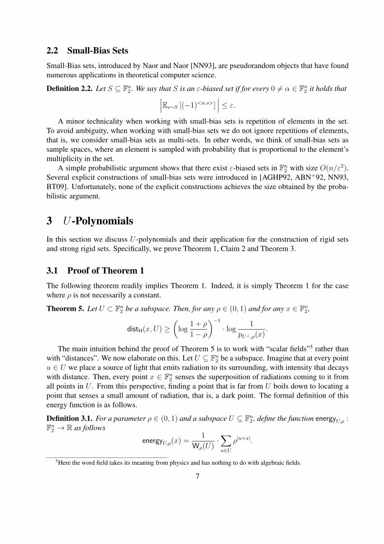
2.2 Small-Bias SetsSmall-Bias sets, introduced by Naor and Naor [NN93], are pseudorandom objects that have foundnumerous applications in theoretical computer science.

Definition 2.2. Let S ⊆ Fn2 . We say that S is an ε-biased set if for every 0 6= α ∈ Fn2 it holds that∣∣∣Es∼S [(−1)<α,s>]∣∣∣ ≤ ε.

A minor technicality when working with small-bias sets is repetition of elements in the set.To avoid ambiguity, when working with small-bias sets we do not ignore repetitions of elements,that is, we consider small-bias sets as multi-sets. In other words, we think of small-bias sets assample spaces, where an element is sampled with probability that is proportional to the element’smultiplicity in the set.

A simple probabilistic argument shows that there exist ε-biased sets in Fn2 with size O(n/ε2).Several explicit constructions of small-bias sets were introduced in [AGHP92, ABN+92, NN93,BT09]. Unfortunately, none of the explicit constructions achieves the size obtained by the proba-bilistic argument.

3 U -PolynomialsIn this section we discuss U -polynomials and their application for the construction of rigid setsand strong rigid sets. Specifically, we prove Theorem 1, Claim 2 and Theorem 3.

3.1 Proof of Theorem 1The following theorem readily implies Theorem 1. Indeed, it is simply Theorem 1 for the casewhere ρ is not necessarily a constant.

Theorem 5. Let U ⊂ Fn2 be a subspace. Then, for any ρ ∈ (0, 1) and for any x ∈ Fn2 ,

distH(x, U) ≥(

log1 + ρ

1− ρ

)−1

· log1

pU⊥,ρ(x).

The main intuition behind the proof of Theorem 5 is to work with “scalar fields”5 rather thanwith “distances”. We now elaborate on this. Let U ⊆ Fn2 be a subspace. Imagine that at every pointu ∈ U we place a source of light that emits radiation to its surrounding, with intensity that decayswith distance. Then, every point x ∈ Fn2 senses the superposition of radiations coming to it fromall points in U . From this perspective, finding a point that is far from U boils down to locating apoint that senses a small amount of radiation, that is, a dark point. The formal definition of thisenergy function is as follows.

Definition 3.1. For a parameter ρ ∈ (0, 1) and a subspace U ⊆ Fn2 , define the function energyU,ρ :Fn2 → R as follows

energyU,ρ(x) =1

Wρ(U)·∑u∈U

ρ|u+x|.

5Here the word field takes its meaning from physics and has nothing to do with algebraic fields.

7

When it is not needed to specify one or more of the parameters ρ, U , we omit them. We notethat energyU(x) ∈ (0, 1], and that energyU(x) = 1 if and only if x ∈ U . (The lower bound isobvious, whereas the upper bound and the characterization of equality follows from equation 3.3below.) Thus, not surprisingly, a maximum amount of radiation is sensed on the subspace U itself.Moreover, for a uniformly sampled x ∈ Fn2 , energyU(x) is exponential in Ω(k − n). That is, atypical point in Fn2 senses a small amount of radiation, and so most of Fn2 is dark.

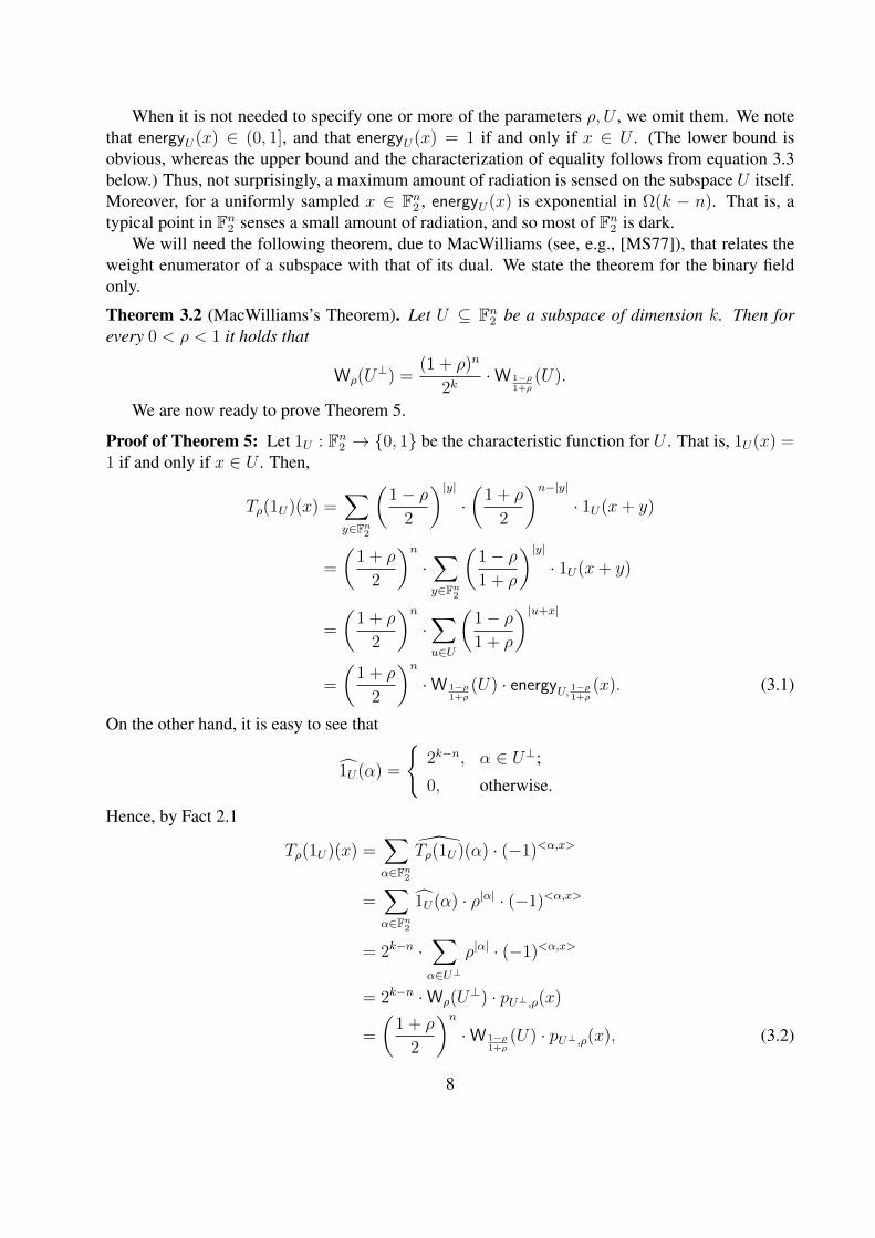
We will need the following theorem, due to MacWilliams (see, e.g., [MS77]), that relates theweight enumerator of a subspace with that of its dual. We state the theorem for the binary fieldonly.

Theorem 3.2 (MacWilliams’s Theorem). Let U ⊆ Fn2 be a subspace of dimension k. Then forevery 0 < ρ < 1 it holds that

Wρ(U⊥) =

(1 + ρ)n

2k·W 1−ρ

1+ρ(U).

We are now ready to prove Theorem 5.

Proof of Theorem 5: Let 1U : Fn2 → 0, 1 be the characteristic function for U . That is, 1U(x) =1 if and only if x ∈ U . Then,

Tρ(1U)(x) =∑y∈Fn2

(1− ρ

2

)|y|·(

1 + ρ

2

)n−|y|· 1U(x+ y)

=

(1 + ρ

2

)n·∑y∈Fn2

(1− ρ1 + ρ

)|y|· 1U(x+ y)

=

(1 + ρ

2

)n·∑u∈U

(1− ρ1 + ρ

)|u+x|

=

(1 + ρ

2

)n·W 1−ρ

1+ρ(U) · energyU, 1−ρ

1+ρ(x). (3.1)

On the other hand, it is easy to see that

1U(α) =

2k−n, α ∈ U⊥;

0, otherwise.

Hence, by Fact 2.1

Tρ(1U)(x) =∑α∈Fn2

Tρ(1U)(α) · (−1)<α,x>

=∑α∈Fn2

1U(α) · ρ|α| · (−1)<α,x>

= 2k−n ·∑α∈U⊥

ρ|α| · (−1)<α,x>

= 2k−n ·Wρ(U⊥) · pU⊥,ρ(x)

=

(1 + ρ

2

)n·W 1−ρ

1+ρ(U) · pU⊥,ρ(x), (3.2)

8

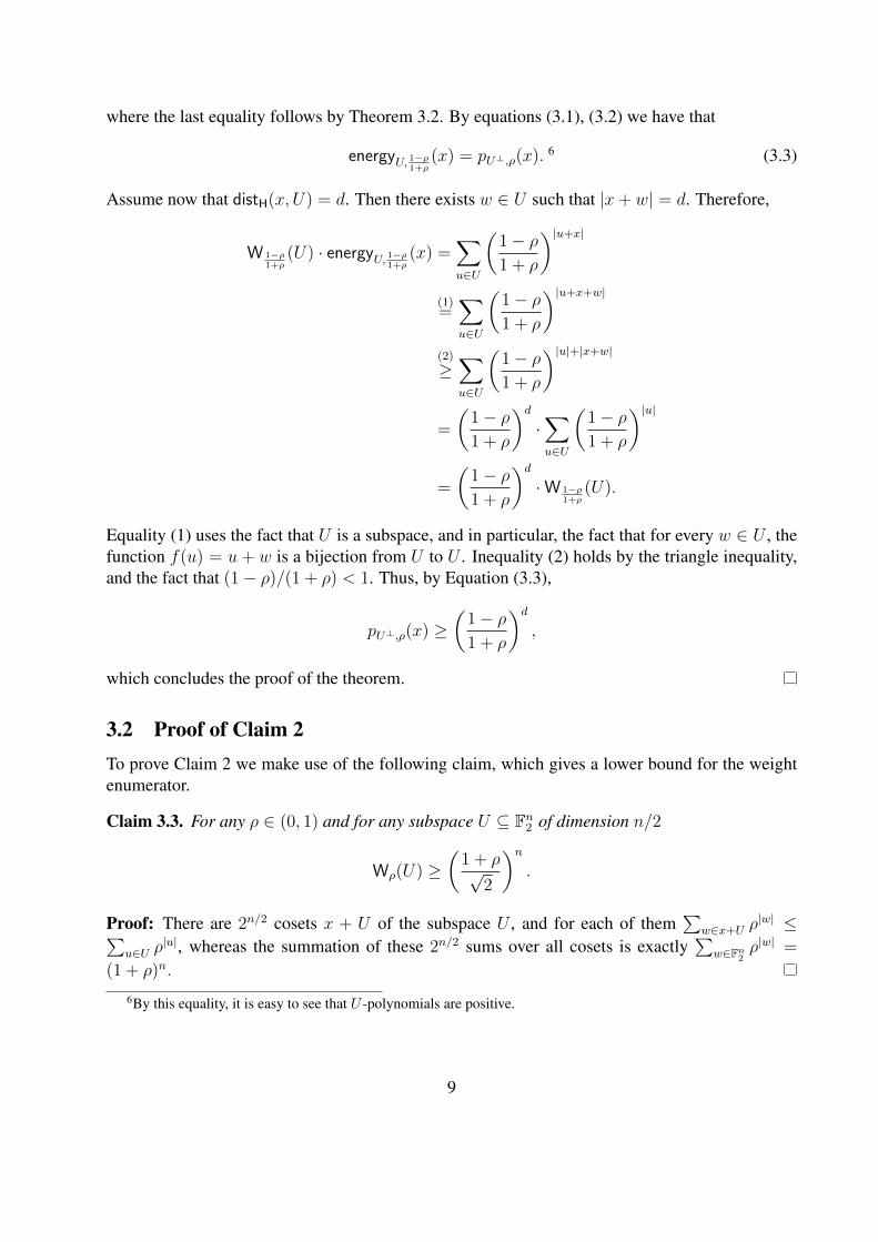
where the last equality follows by Theorem 3.2. By equations (3.1), (3.2) we have that

energyU, 1−ρ1+ρ

(x) = pU⊥,ρ(x). 6 (3.3)

Assume now that distH(x, U) = d. Then there exists w ∈ U such that |x+ w| = d. Therefore,

W 1−ρ1+ρ

(U) · energyU, 1−ρ1+ρ

(x) =∑u∈U

(1− ρ1 + ρ

)|u+x|

(1)=∑u∈U

(1− ρ1 + ρ

)|u+x+w|

(2)

≥∑u∈U

(1− ρ1 + ρ

)|u|+|x+w|

=

(1− ρ1 + ρ

)d·∑u∈U

(1− ρ1 + ρ

)|u|=

(1− ρ1 + ρ

)d·W 1−ρ

1+ρ(U).

Equality (1) uses the fact that U is a subspace, and in particular, the fact that for every w ∈ U , thefunction f(u) = u + w is a bijection from U to U . Inequality (2) holds by the triangle inequality,and the fact that (1− ρ)/(1 + ρ) < 1. Thus, by Equation (3.3),

pU⊥,ρ(x) ≥(

1− ρ1 + ρ

)d,

which concludes the proof of the theorem.

3.2 Proof of Claim 2To prove Claim 2 we make use of the following claim, which gives a lower bound for the weightenumerator.

Claim 3.3. For any ρ ∈ (0, 1) and for any subspace U ⊆ Fn2 of dimension n/2

Wρ(U) ≥(

1 + ρ√2

)n.

Proof: There are 2n/2 cosets x + U of the subspace U , and for each of them∑

w∈x+U ρ|w| ≤∑

u∈U ρ|u|, whereas the summation of these 2n/2 sums over all cosets is exactly

∑w∈Fn2

ρ|w| =

(1 + ρ)n.

6By this equality, it is easy to see that U -polynomials are positive.

9

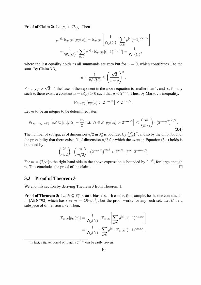
Proof of Claim 2: Let pU ∈ Pn/2. Then

µ , Ex∼Fn2 [pU(x)] = Ex∼Fn2

[1

Wρ(U)·∑u∈U

ρ|u|(−1)<u,x>

]

=1

Wρ(U)·∑u∈U

ρ|u| · Ex∼Fn2 [(−1)<u,x>] =1

Wρ(U),

where the last equality holds as all summands are zero but for u = 0, which contributes 1 to thesum. By Claim 3.3,

µ =1

Wρ(U)≤

( √2

1 + ρ

)n

.

For any ρ >√

2−1 the base of the exponent in the above equation is smaller than 1, and so, for anysuch ρ, there exists a constant α = α(ρ) > 0 such that µ < 2−αn. Thus, by Markov’s inequality,

Prx∼Fn2[pU(x) > 2−αn/2

]≤ 2−αn/2.

Let m to be an integer to be determined later.

Prx1,...,xm∼Fn2

[∃S ⊆ [m], |S| = m

2s.t. ∀i ∈ S pU(xi) > 2−αn/2

]≤(m

m/2

)·(2−αn/2

)m/2.

(3.4)The number of subspaces of dimension n/2 in Fn2 is bounded by

(2n

n/2

)7, and so by the union bound,

the probability that there exists U of dimension n/2 for which the event in Equation (3.4) holds isbounded by (

2n

n/2

)·(m

m/2

)·(2−αn/2

)m/2< 2n

2/2 · 2m · 2−αnm/4.

For m = (7/α)n the right hand side in the above expression is bounded by 2−n2 , for large enough

n. This concludes the proof of the claim.

3.3 Proof of Theorem 3We end this section by deriving Theorem 3 from Theorem 1.

Proof of Theorem 3: Let S ⊆ Fn2 be an ε-biased set. It can be, for example, be the one constructedin [ABN+92] which has size m = O(n/ε3), but the proof works for any such set. Let U be asubspace of dimension n/2. Then,

Ex∼S[pU(x)] =1

Wρ(U)· Ex∼S

[∑u∈U

ρ|u| · (−1)<u,x>

]

=1

Wρ(U)·∑u∈U

ρ|u| · Ex∼S [(−1)<u,x>].

7In fact, a tighter bound of roughly 2n2/4 can be easily proven.

10

Any summand except for u = 0 is bounded in absolute value by ε. Thus,

Ex∼S[pU(x)] < ε+1

Wρ(U).

Assume for now that we will pick ε > 1/Wρ(U), and so we can further simplify to get Ex∼S[pU(x)] <2ε. Since log(1/x) is a convex function, we get, by Jensen’s inequality that

Ex∼S[log

(1

pU(x)

)]≥ log

(1

Ex∼S[pU(x)]

)≥ log

(1

2ε

).

Since we are working with subspaces of dimension n/2, the above equation also holds for thedual of every subspace of dimension n/2. Thus, by Theorem 1, for every subspace U ⊂ Fn2 withdimension n/2

Ex∼S [distH(x, U)] = Ω

(log

1

ε

).

Recall that in our case m = O(n/ε3), and so setting m = n · 2Θ(d) would give that S is an(n, n/2, d)-strong rigid set with size m.

We now return to the assumption we made, namely, that ε > 1/Wρ(U). Eventually we choseε = exp(−d), and so to justify the assumption, it is enough to show that Wρ(U) > exp(d). ByClaim 3.3 we have that Wρ(U) ≥ ((1 + ρ)/

√2)n. For ρ >

√2 − 1, the base of the exponent is

larger than 1. For any such ρ, there exists a constant c = c(ρ) > 0 such that our assumption is metas long as d ≤ c · n.

4 Strong Rigid Sets from Small-Bias Sets - Alternative ProofsIn this section we give two alternative proofs for Theorem 3. We refer to the two proofs as thebias-reduction proof and the covering proof.

4.1 The Bias-Reduction ProofThis proof relies on the Parity Lemma (c.f., for example, [NN93]).

Lemma 4.1 (The Parity Lemma). Let S ⊆ 0, 1n be an ε-biased set. Let T ⊆ [n] be a non-emptyset of size k. Denote by ST the projection of S on the index set T . Then,

SD(ST ,Uk) ≤ ε · 2k/2.

Lemma 4.1 roughly states that the projection of a small-bias set on a small number of coordi-nates is close, in statistical distance, to the uniform distribution. Since a random vector is, withhigh probability, far from any given subspace with small dimension, one would hope that a typicalvector in a small-bias set would also be far from any given subspace. This idea fails because al-though the bound on the statistical distance guaranteed by the Parity Lemma depends linearly onthe bias of the small-bias set, it depends exponentially on n, the length of the vectors.

A natural suggestion for circumventing this problem is to partition the set of indices [n] toblocks and apply the argument above for each block separately. This way, the statistical distance

11

guaranteed by the Parity Lemma will be exponential in the block length, which can be controlled,as opposed to being exponential in n. However, this suggestion fails as well since one must takethe block size large enough so that the projection of the subspace on a block would still havesmall dimension with respect to the block length. Indeed, otherwise a random vector would notnecessarily be far from the projection.

As mentioned, the statistical distance guaranteed by the Parity Lemma depends linearly on thebias of the small-bias set and exponentially on n. The natural idea above tried to obtain a betterguarantee on the statistical distance by decreasing the exponential part as it naturally seems tocause the problem. However, this idea failed. The idea behind the “bias-reduction proof” as itsname suggests, is to reduce the bias enough so as to cancel the exponential loss incurred by theParity Lemma. The way we reduce the bias is by applying the above argument not to the originalsmall-bias set S, but rather to the set S + · · ·+ S, where the number of summands depends on thedistance, d, that we want to achieve. The bias of this sum decreases exponentially with the numberof summands (see Claim 4.2 below). This cancels out the exponential loss we absorb by the ParityLemma, as desired. This shows that S + · · · + S is a strong rigid set with good parameters. Wethen show that this implies that S itself must also be a strong rigid set (with weaker parameters).We now make this formal. We need the following claim.

Claim 4.2. Let S be an ε-biased set. Then, for every integer c ≥ 1, c · S is an εc-biased set.

Proof: For any 0 6= α ∈ Fn2

|Ex∼c·S [(−1)<α,x>]| =∣∣Es1,...,sc∼S [(−1)<α,s1+···+sc>

]∣∣=

∣∣∣∣∣Es1,...,sc∼S[

c∏i=1

(−1)<α,si>

]∣∣∣∣∣=

c∏i=1

|Esi∼S [(−1)<α,si>]| ≤ εc.

We are now ready to give the bias-reduction proof for Theorem 3.

Proof of Theorem 3: Let S be a 2−c′d-biased set for a constant c′ > 0 to be determined later on.

Let S ′ = (n/20d) · S. By Claim 4.2, S ′ is a 2−c′n/20-biased set. Let U ⊂ Fn2 be a subspace of

dimension n/2. By standard counting arguments one can show that

Prx∼Fn2

[distH(x, U) >

n

10

]> 0.6.

By the Parity Lemma (Lemma 4.1), we have that

SD (S ′,Fn2 ) ≤ 2−c′n/20+n/2 < 0.1,

where the last inequality holds for a sufficiently large constant c′. We choose c′ accordingly. Thus,

Prx∼S′[distH(x, U) >

n

10

]> 0.5.

12

In particular, the latter implies that

Ex∼S′ [distH(x, U)] >n

20.

Recall that S ′ = (n/20d) · S, and so the above equation can be written as

Es1,...,sn/20d∼S

distHn/20d∑

i=1

si, U

> n

20. (4.1)

At this point we note that for every s1, . . . , sn/20d ∈ S

n/20d∑i=1

distH(si, U) ≥ distH

n/20d∑i=1

si, U

.

Indeed, for i ∈ [n/20d], let ui ∈ U be such that distH(si, U) = |si + ui|. Then,

n/20d∑i=1

distH(si, U) =

n/20d∑i=1

|si + ui| ≥

∣∣∣∣∣∣n/20d∑i=1

si +

n/d∑i=1

ui

∣∣∣∣∣∣ ≥ distH

n/20d∑i=1

si, U

,

where the last inequality follows since U is closed under addition. Plugging this into Equation (4.1)and using linearity of expectation, we get

Es∼S[distH (s, U)] > d.

4.2 The Covering ProofIn this section we give a third proof for Theorem 3. We need some preliminary definitions andresults regarding expander graphs. For more information regarding expander graphs we refer thereader to the survey by Hoory, Linial and Wigderson [HLW06].

Let G = (V,E) be an undirected D-regular graph on N vertices. Let AG be the normalizedadjacency matrix of G. That is, for u, v ∈ V , (AG)uv equals the number of edges connecting thevertices u, v, divided by D. It is well-known that the eigenvalues of AG are all real numbers, andthat the maximum eigenvalue is 1. The graph G is called (N,D, λ)-expander if the second largesteigenvalue in absolute value is at most λ.

For a subset S ⊂ V , let e(S) be the number of edges in the induced subgraph of G on S. Thequantity e(S) measures the density of this induced subgraph. In [AC88] Alon and Chung provedthe following lemma, which states that induced subgraphs of expanders have approximately the“right” density.

Theorem 4.3 (Lemma 2.3 in [AC88]). Let G = (V,E) be an (N,D, λ)-expander. Then, for anyset S ⊆ V with size |S| = αN∣∣∣∣e(S)− 1

2Dα2N

∣∣∣∣ ≤ 1

2λDα(1− α)N.

13

We also need the following theorem proved in [AR94].

Theorem 4.4. Let S ⊆ Fn2 be an ε-biased set. Define the graph GS = (V,E) as follows. V = Fn2 ,and an edge connects a pair of vertices u, v if and only if u + v ∈ S. Then, GS is a (2n, |S|, ε)-expander.

With the two theorems above we are ready to prove the following lemma. A similar lemmawas proved by Arvind and Srinivasan [AS10]. Here we give a somewhat simpler proof.

Lemma 4.5. Let S ⊆ Fn2 be an ε-biased set. Then, for any subspace U ⊆ Fn2 of dimension k

|S ∩ U ||S|

≤ 2k−n + ε.

Proof: Define the graph GS = (V,E) as in Theorem 4.4. That is V = Fn2 , and an edge connectsa pair of vertices u, v if and only if u+ v ∈ S. By Theorem 4.4, GS is a (2n, |S|, ε)-expander. LetU ⊂ Fn2 = V be a subspace of dimension k. For u ∈ U , the degree of u in the induced subgraphof GS on U is

|s ∈ S : u+ s ∈ U| = |s ∈ S : s ∈ U| = |U ∩ S|.Thus,

|e(S)| = 1

2· |U | · |U ∩ S|.

By Theorem 4.3,

|U | · |U ∩ S| ≤ |S| ·(|U |2n

)2

· 2n + ε · |S| · |U |,

or equivalently,|U ∩ S||S|

≤ |U |2n

+ ε,

which concludes the proof of the lemma as |U | = 2k.

Proof of Theorem 3: Let U ⊂ Fn2 be a subspace of dimension n/2. We now describe the coveringof the neighborhood of U , proposed in [APY09]. Partition the n unit vectors of Fn2 into 8d setsB1, . . . , B8d of size n/8d each. For every set I ⊆ [8d] with size |I| = 2d, define

UI = Span

(U ∪

⋃i∈I

Bi

).

We note that dim(UI) ≤ 3n/4 for every I , as we add to U , which has dimension n/2, (n/8d) · 2dunit vectors, thus increasing U ’s dimension by at most n/4. Moreover, it is easy to see that everyvector x satisfying distH(x, U) ≤ 2d is contained in UI for some I . Let S be an ε-biased set. ByLemma 4.5, for every I as above,

|S ∩ UI | ≤ |S| ·(2−n/4 + ε

).

There are(

8d2d

)< 120d such sets I , and as mentioned, they cover the 2d-neighborhood of U .

Therefore, S intersects the 2d-neighborhood of U in at most 120d · |S| ·(2−n/4 + ε

)vectors. As

we assume d ≤ c · n, for small enough constant c, setting ε = 120−d/4 implies that at most half ofthe vectors in S are contained in the 2d-neighborhood of U . Thus,

Es∼S [distH(s, U)] ≥ d.

14

5 Rigid Sets from Unbalanced ExpandersIn this section we prove Theorem 4. First we give some preliminary definitions and results regard-ing bipartite expanders. For more information we refer the reader to [HLW06]. Let G = (L,R,E)be a bipartite graph with |L| = m, |R| = n, and left-degree d. For a set S ⊆ L define

Γ(S) = r ∈ R : ∃s ∈ S such that sr ∈ E,

andΓ1(S) = r ∈ R : ∃!s ∈ S such that sr ∈ E.

G is called (kmax, 1− ε)-bipartite-expander if for every S ⊆ L with size at most kmax, it holdsthat |Γ(S)| ≥ (1− ε)d|S|. G is called (kmax, 1− ε)-unique neighbor expander if for every S ⊆ Lwith size at most kmax, it holds that |Γ1(S)| ≥ (1− ε)d|S|. The following simple well known factrelates the two definitions.

Fact 5.1. Every (kmax, 1− ε)-bipartite expander is a (kmax, 1− 2ε)-unique neighbor expander.

We will be interested in the case where m >> n. Such bipartite expanders are called unbal-anced expanders. It can be shown, using a standard probabilistic argument, that for every n, d, kmax

such that kmax = O(n/d) and for every constant ε > 0, there exists a (kmax, 1−ε)-bipartite expanderwith

m = kmax ·(

n

d · kmax

)Ω(d)

.

In particular, by Fact 5.1, this bipartite expander is a (kmax, 1− 2ε)-unique neighbor expander. Thestate of the art explicit construction for unbalanced expanders is due to Guruswami et al. [GUV09].Unfortunately, it falls short of achieving the same parameters as the probabilistic constructionabove. We are now ready to prove Theorem 4.

Proof of Theorem 4: By Fact 5.1, we have that G is a (kmax, 1/3)-unique neighbor expander. LetU ⊆ Fn2 be a subspace of dimension k. Assume for contradiction that for every c ∈ C there existsuc ∈ U such that |c + uc| ≤ d. In case there is more than one element in U that is of distance atmost d from c, we choose one such element arbitrarily. Define U ′ = uc : c ∈ C.

Claim 5.2. |U ′| = |C| = m

Proof: Let c, c′ be two distinct elements in C. To prove the claim it is enough to show thatuc 6= uc′ . Assume for contradiction that uc = uc′ . Then, by the triangle inequality,

|c+ c′| ≤ |c+ uc|+ |c′ + uc′|+ |uc + uc′ | ≤ 2d. (5.1)

On the other hand, G is a (kmax, 1/3)-unique neighbor expander. Hence,

|c+ c′| ≥ 1

3· 4d · 2 > 2d,

contradicting Equation (5.1).

15

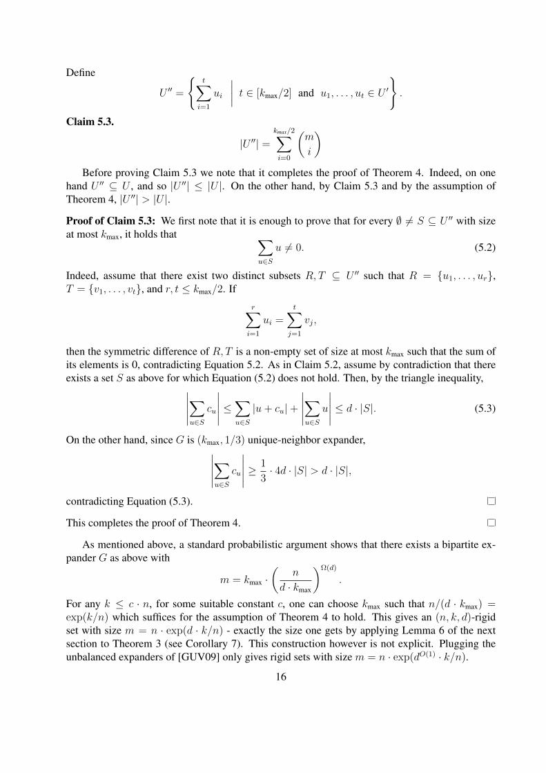
Define

U ′′ =

t∑i=1

ui

∣∣∣∣ t ∈ [kmax/2] and u1, . . . , ut ∈ U ′.

Claim 5.3.

|U ′′| =kmax/2∑i=0

(m

i

)Before proving Claim 5.3 we note that it completes the proof of Theorem 4. Indeed, on one

hand U ′′ ⊆ U , and so |U ′′| ≤ |U |. On the other hand, by Claim 5.3 and by the assumption ofTheorem 4, |U ′′| > |U |.

Proof of Claim 5.3: We first note that it is enough to prove that for every ∅ 6= S ⊆ U ′′ with sizeat most kmax, it holds that ∑

u∈S

u 6= 0. (5.2)

Indeed, assume that there exist two distinct subsets R, T ⊆ U ′′ such that R = u1, . . . , ur,T = v1, . . . , vt, and r, t ≤ kmax/2. If

r∑i=1

ui =t∑

j=1

vj,

then the symmetric difference of R, T is a non-empty set of size at most kmax such that the sum ofits elements is 0, contradicting Equation 5.2. As in Claim 5.2, assume by contradiction that thereexists a set S as above for which Equation (5.2) does not hold. Then, by the triangle inequality,∣∣∣∣∣∑

u∈S

cu

∣∣∣∣∣ ≤∑u∈S

|u+ cu|+

∣∣∣∣∣∑u∈S

u

∣∣∣∣∣ ≤ d · |S|. (5.3)

On the other hand, since G is (kmax, 1/3) unique-neighbor expander,∣∣∣∣∣∑u∈S

cu

∣∣∣∣∣ ≥ 1

3· 4d · |S| > d · |S|,

contradicting Equation (5.3).

This completes the proof of Theorem 4.

As mentioned above, a standard probabilistic argument shows that there exists a bipartite ex-pander G as above with

m = kmax ·(

n

d · kmax

)Ω(d)

.

For any k ≤ c · n, for some suitable constant c, one can choose kmax such that n/(d · kmax) =exp(k/n) which suffices for the assumption of Theorem 4 to hold. This gives an (n, k, d)-rigidset with size m = n · exp(d · k/n) - exactly the size one gets by applying Lemma 6 of the nextsection to Theorem 3 (see Corollary 7). This construction however is not explicit. Plugging theunbalanced expanders of [GUV09] only gives rigid sets with size m = n · exp(dO(1) · k/n).

16

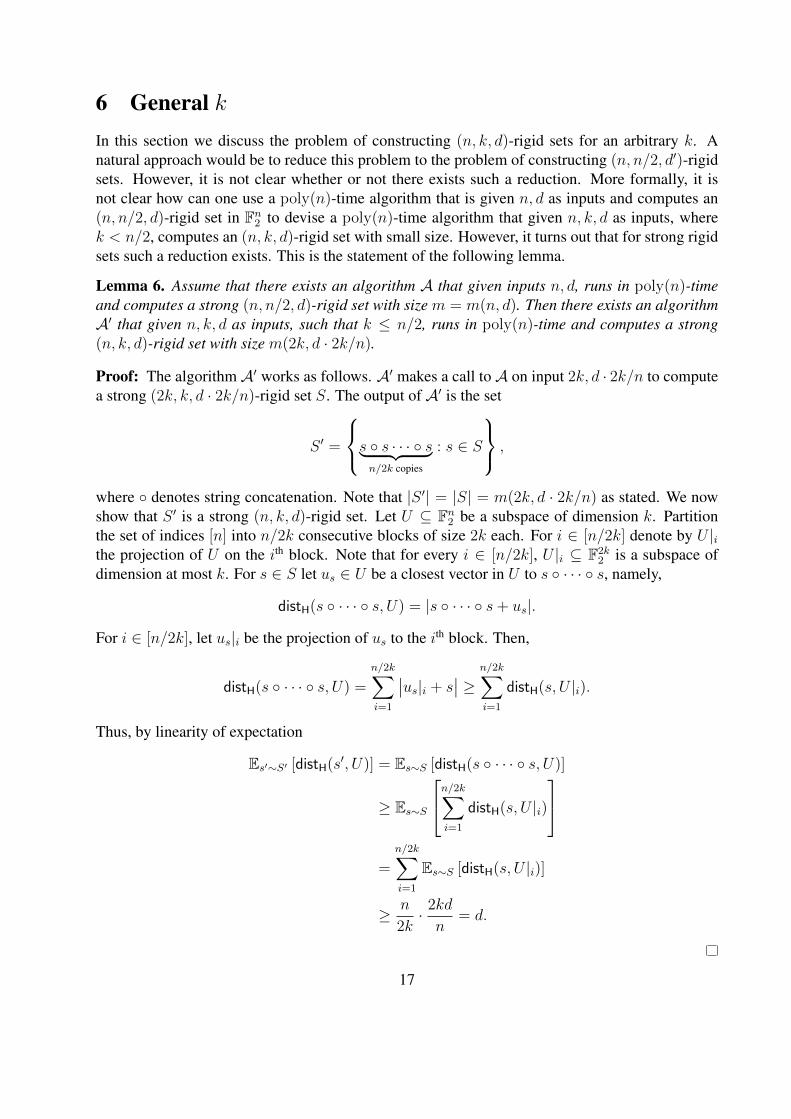
6 General kIn this section we discuss the problem of constructing (n, k, d)-rigid sets for an arbitrary k. Anatural approach would be to reduce this problem to the problem of constructing (n, n/2, d′)-rigidsets. However, it is not clear whether or not there exists such a reduction. More formally, it isnot clear how can one use a poly(n)-time algorithm that is given n, d as inputs and computes an(n, n/2, d)-rigid set in Fn2 to devise a poly(n)-time algorithm that given n, k, d as inputs, wherek < n/2, computes an (n, k, d)-rigid set with small size. However, it turns out that for strong rigidsets such a reduction exists. This is the statement of the following lemma.

Lemma 6. Assume that there exists an algorithm A that given inputs n, d, runs in poly(n)-timeand computes a strong (n, n/2, d)-rigid set with size m = m(n, d). Then there exists an algorithmA′ that given n, k, d as inputs, such that k ≤ n/2, runs in poly(n)-time and computes a strong(n, k, d)-rigid set with size m(2k, d · 2k/n).

Proof: The algorithm A′ works as follows. A′ makes a call to A on input 2k, d · 2k/n to computea strong (2k, k, d · 2k/n)-rigid set S. The output of A′ is the set

S ′ =

s s · · · s︸ ︷︷ ︸n/2k copies

: s ∈ S

,

where denotes string concatenation. Note that |S ′| = |S| = m(2k, d · 2k/n) as stated. We nowshow that S ′ is a strong (n, k, d)-rigid set. Let U ⊆ Fn2 be a subspace of dimension k. Partitionthe set of indices [n] into n/2k consecutive blocks of size 2k each. For i ∈ [n/2k] denote by U |ithe projection of U on the ith block. Note that for every i ∈ [n/2k], U |i ⊆ F2k

2 is a subspace ofdimension at most k. For s ∈ S let us ∈ U be a closest vector in U to s · · · s, namely,

distH(s · · · s, U) = |s · · · s+ us|.

For i ∈ [n/2k], let us|i be the projection of us to the ith block. Then,

distH(s · · · s, U) =

n/2k∑i=1

∣∣us|i + s∣∣ ≥ n/2k∑

i=1

distH(s, U |i).

Thus, by linearity of expectation

Es′∼S′ [distH(s′, U)] = Es∼S [distH(s · · · s, U)]

≥ Es∼S

n/2k∑i=1

distH(s, U |i)

=

n/2k∑i=1

Es∼S [distH(s, U |i)]

≥ n

2k· 2kd

n= d.

17

Theorem 3 together with Lemma 6 yield the following corollary.

Corollary 7. Let n, k, d be such that k ≤ n/2 and d ≤ c · n for some suitable constant 0 < c < 1.Then there exists an explicit construction of an (n, k, d)-strong rigid set with size n · exp(d · k/n).

In fact, one can generalize each of the proofs we gave for Theorem 3 to show that an exp(−d ·k/n)-biased set is an (n, k, d)-strong rigid set. Nevertheless, the reduction in Lemma 6 might beof use in the construction of (n, k, d)-strong rigid sets from arbitrary (n, n/2, d)-rigid sets.

AcknowledgementsThe second author is grateful for his advisor Ran Raz for his continuous support and encourage-ment, and for helpful discussions regarding this work. He would also like to thank Amir Shpilka forintroducing him to the paper [APY09] and Avraham Ben-Aroya and Igor Shinkar for stimulatingdiscussions.

References[ABN+92] N. Alon, J. Bruck, J. Naor, M. Naor, and R. Roth. Construction of asymptotically good

low-rate error-correcting codes through pseudo-random graphs. IEEE Transactionson Information Theory, 38:509–516, 1992.

[AC88] N. Alon and F.R.K. Chung. Explicit construction of linear sized tolerant networks.Discrete Mathematics, 72(1):15–19, 1988.

[AGHP92] N. Alon, O. Goldreich, J. Hastad, and R. Peralta. Simple construction of almostk-wise independent random variables. Random Structures and Algorithms, 3(3):289–304, 1992.

[APY09] N. Alon, R. Panigrahy, and S. Yekhanin. Deterministic approximation algorithmsfor the nearest codeword problem. In APPROX 09 / RANDOM 09: Proceedings ofthe 12th International Workshop and 13th International Workshop on Approximation,Randomization, and Combinatorial Optimization. Algorithms and Techniques, pages339–351, 2009.

[AR94] N. Alon and Y. Roichman. Random cayley graphs and expanders. Random Structuresand Algorithms, 5(2):271–285, 1994.

[AS10] V. Arvind and S. Srinivasan. The remote point problem, small bias spaces, and ex-panding generator sets. In 27th STACS, pages 59–70, 2010.

[BDWY11] B. Barak, Z. Dvir, A. Wigderson, and A. Yehudayoff. Rank bounds for design ma-trices with applications to combinatorial geometry and locally correctable codes. InProceedings of the 43rd annual ACM symposium on Theory of computing, pages 519–528. ACM, 2011.

18

[BT09] A. Ben-Aroya and A. Ta-Shma. Constructing small-bias sets from algebraic-geometric codes. In Proceedings of the 50th annual IEEE symposium on foundationsof computer science (FOCS), pages 191–197, 2009.

[Dvi10] Z. Dvir. On matrix rigidity and locally self-correctable codes. In Proceedings of the25th Annual CCC, pages 291–298, 2010.

[Fri93] J. Friedman. A note on matrix rigidity. Combinatorica, 13(2):235–239, 1993.

[GUV09] V. Guruswami, C. Umans, and S. Vadhan. Unbalanced expanders and randomnessextractors from Parvaresh–Vardy codes. J. ACM, 56(4):1–34, 2009.

[HLW06] S. Hoory, N. Linial, and A. Wigderson. Expander graphs and their applications. Bul-leting of the American Mathematical Society, 43:439–561, 2006.

[KR98] B.S. Kashin and A.A. Razborov. Improved lower bounds on the rigidity of Hadamardmatrices. Mathematical Notes, 63(4):471–475, 1998.

[Lok95] S. V. Lokam. Spectral methods for matrix rigidity with applications to size-depthtradeoffs and communication complexity. In 36th Annual FOCS, pages 6–15, 1995.

[Lok09] S. V. Lokam. Complexity lower bounds using linear algebra. Foundations and Trendsin Theoretical Computer Science, 4(1-2):1–155, 2009.

[MS77] F. J. MacWilliams and N. J. A. Sloane. The Theory of Error-Correcting Codes, PartII. North-Holland, 1977.

[NN93] J. Naor and M. Naor. Small-bias probability spaces: Efficient constructions and ap-plications. SIAM J. on Computing, 22(4):838–856, 1993.

[O’D] R. O’Donnell. Analyis of boolean functions. http://analysisofbooleanfunctions.org/.

[SSS97] M.A. Shokrollahi, D. Spielman, and V. Stemann. A remark on matrix rigidity. Infor-mation Processing Letters, 64(6):283–285, 1997.

[Val77] L. G. Valiant. Graph-theoretic arguments in low-level complexity. In Lecture notesin Computer Science, volume 53, pages 162–176. Springer, 1977.

19