Step 4 – Applying the Boundary Conditions The global system of equations :The global system of...

4/13/2012

1

Discrete systems

Steps of the Finite Element Method

1. Discretizing the domaing

subdividing the domain into elements and nodes

For discrete systems like trusses and frames the system is already discretized and this step isunnecessary. In this case the answers obtained areexact.

For continuous systems like plates and shells this stepbecomes very important and the answers obtained areonly approximate. In this case, the accuracy of thesolution depends on the discretization used.

4/13/2012

2

2. Writing the element stiffness matrices

The element stiffness equations need to be writtenThe element stiffness equations need to be writtenfor each element in the domain. This step will beperformed using MATLAB.

3. Assembling the global stiffness matrix

Thi ill b d i th di t tiffThis will be done using the direct stiffnessapproach. This step will be performed usingMATLAB.

4. Applying the boundary conditions

like supports and applied loads and displacements.

5. Solving the equations

This will be done by partitioning the global stiffnessmatrix and then solving the resulting equationsusing MATLAB with Gaussian elimination.

6. Post‐processing

To obtain additional information like the reactionsand element forces and stresses.

4/13/2012

3

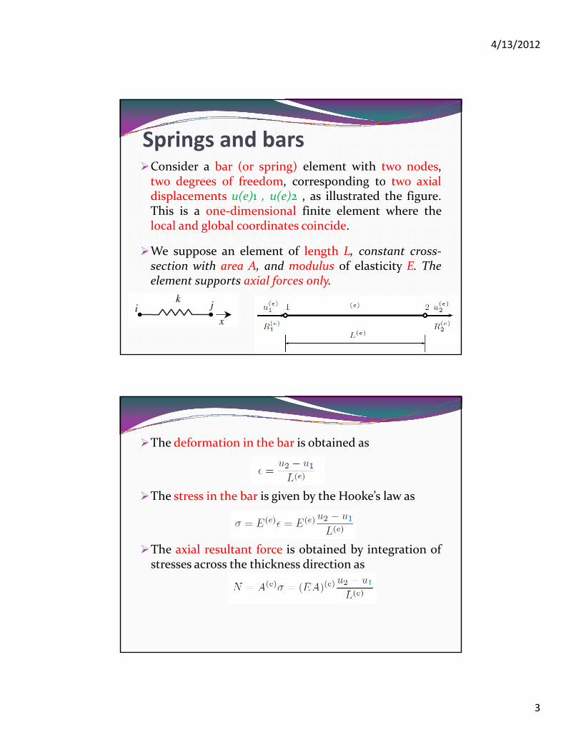
Springs and barsConsider a bar (or spring) element with two nodes,two degrees of freedom, corresponding to two axialtwo degrees of freedom, corresponding to two axialdisplacements u(e)1 , u(e)2 , as illustrated the figure.This is a one‐dimensional finite element where thelocal and global coordinates coincide.

We suppose an element of length L, constant cross‐section with area A, and modulus of elasticity E. Thesection with a ea , and modulus o e ast c ty . heelement supports axial forces only.

The deformation in the bar is obtained as

The stress in the bar is given by the Hooke’s law as

The axial resultant force is obtained by integration ofstresses across the thickness direction asstresses across the thickness direction as

4/13/2012

4

Taking into account the static equilibrium of the axial forces

We can write the equations in the form (taking k(e) = EA/L )q ( g ( ) / )

where K(e) is the stiffness matrix of the bar (spring) element,a(e) is the displacement vector, and q(e) represents the vector ofnodal forces.

If the element undergoes the action of distributed forces, it isnecessary to transform those forces into nodal forces, by

Equilibrium at nodes

W d bl h ib i f ll lWe need to assemble the contribution of all elementsso that a global system of equations can be obtained.

To do that we recall that in each node the sum of allforces arising from various adjacent elementsforces arising from various adjacent elementsequals the applied load at that node.

4/13/2012

5

We then obtain

producing a global system of equations in the form

Or in a more compact form

Here K represents the system (or structure) stiffnessmatrix, a is the system displacement vector, and frepresents the system force vector.

Some basic steps1. Define a set of elements connected at nodes or

Discretizing the Domain.Discretizing the Domain.

2. For each element, compute stiffness matrix K(e), andforce vector f (e)

3. Assemble the contribution of all elements into the globalsystem Ka = f

4. Modify the global system by imposing essential(di l t ) b d diti(displacements) boundary conditions

5. Solve the global system and obtain the globaldisplacements a

6. For each element, evaluate the strains and stresses (post‐processing)

4/13/2012

6

Example 1:Consider the two‐element spring system shown in theConsider the two element spring system shown in theFigure. Given k1 = 100 kN/m, k2 = 200 kN/m, and P = 15 kN,determine:

1. the global stiffness matrix for the system.

2. the displacements at nodes 2 and 3.p 3

3. the reaction at node 1.

4. the force in each spring.

Solution: Step 1 – Discretizing the Domain:

Step 2 –Writing the Element Stiffness Matrices:The two element stiffness matrices k1 and k2 are obtained by makingcalls to the MATLAB function SpringElementStiffness. Each matrix hassize 2 × 2.

function y = SpringElementStiffness(k)%SpringElementStiffness This function returns the element stiffness% matrix for a spring with stiffness k.% The size of the element stiffness matrix% is 2 x 2.y = [k –k; –k k];

4/13/2012

7

» k1=SpringElementStiffness(100)

k1 =

100 ‐100

‐100 100

» k2=SpringElementStiffness(200)

k2 =k2

200 ‐200

‐200 200

Step 3 – Assembling the Global Stiffness Matrix:

Since the spring system has three nodes, the size of the global stiffness matrix is3×3. Therefore to obtain K we first set up a zero matrix of size 3 × 3 then maketwo calls to the MATLAB function SpringAssemble.

function y = SpringAssemble(K,k,i,j)

%SpringAssemble This function assembles the element stiffness

% matrix k of the spring with nodes i and j into the

% global stiffness matrix K.

% This function returns the global stiffness matrix K

% after the element stiffness matrix k is assembled% after the element stiffness matrix k is assembled.

K(i,i) = K(i,i) + k(1,1);

K(i,j) = K(i,j) + k(1,2);

K(j,i) = K(j,i) + k(2,1);

K(j,j) = K(j,j) + k(2,2);

y = K;

4/13/2012

8

» K=zeros(3,3)K =

0 0 00 0 00 0 00 0 0

» K=SpringAssemble(K,k1,1,2)K =

100 ‐100 0‐100 100 00 0 0


100 ‐100 0‐100 300 ‐2000 ‐200 200

Step 4 – Applying the Boundary Conditions

The global system of equations :The global system of equations :

The boundary conditions:

Thus :

4/13/2012

9

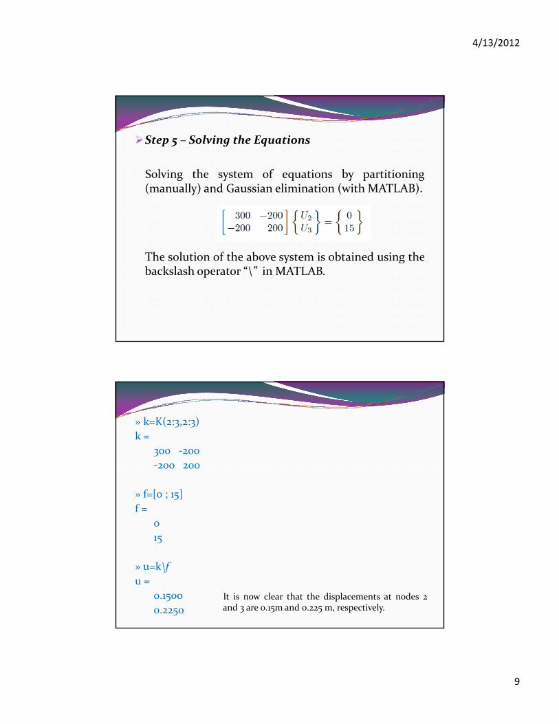
Step 5 – Solving the Equations

Solving the system of equations by partitioningSolving the system of equations by partitioning(manually) and Gaussian elimination (with MATLAB).

The solution of the above system is obtained using theThe solution of the above system is obtained using thebackslash operator “\” in MATLAB.

» k=K(2:3,2:3)

k =

300 ‐200

200 200‐200 200

» f=[0 ; 15]

f =

0

15

» u=k\f

u =

0.1500

0.2250

It is now clear that the displacements at nodes 2and 3 are 0.15m and 0.225 m, respectively.

4/13/2012

10

Step 6 – Post‐processing:

The reaction at node 1 and the force in each spring usingMATLAB are obtained. First we set up the global nodaldisplacement vector U, then we calculate the global nodalforce vector Fforce vector F.

» U=[0 ; u]U =

00.15000.2250

» F=K*UF =

‐15015

Finally we set up the element nodal displacement vectors u1and u2, then we calculate the element force vectors f1 and f2by making calls to the MATLAB functionSpringElementForcesSpringElementForces.

function y = SpringElementForces(k,u)

%SpringElementForces This function returns the

% element nodal force vector

% given the element stiffness% given the element stiffness

% matrix k and the element

% nodal displacement vector u.

y = k * u;

4/13/2012

11

» u1=[0 ; U(2)]u1 =

00.1500

» f1=SpringElementForces(k1,u1)f1 =

‐1515

» u2=[U(2) ; U(3)]u2 =

0.15000.2250


‐1515

It is clear that the force in element 1 is 15 kN(tensile) and the force in element 2 is also 15kN (tensile).

Example 2Consider the spring system composed of six springs as Consider the spring system composed of six springs as shown in the figure Given k = 120 kN/m and P = 20kN, determine:

1. the global stiffness matrix for the system.

2. the displacements at nodes 3, 4, and 5.p 3 4 5

3. the reactions at nodes 1 and 2.

4. the force in each spring.

4/13/2012

12

SolutionStep 1 – Discretizing the DomainStep 1 Discretizing the Domain

Step 2 –Writing the Element Stiffness MatricesThe six element stiffness matrices k1, k2, k3, k4, k5, and k6are obtained by making calls to the MATLAB functionSpringElementStiffness. Each matrix has size 2 × 2.

» k1=SpringElementStiffness(120)k1 =

120 ‐120‐120 120

.

.

.

» k6=SpringElementStiffness(120)k6 =

120 ‐120‐120 120

4/13/2012

13

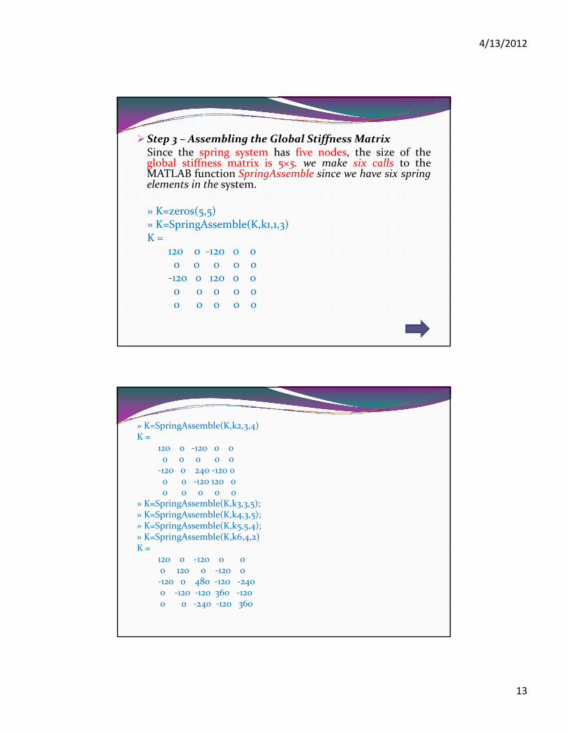
Step 3 – Assembling the Global Stiffness MatrixSince the spring system has five nodes, the size of theglobal stiffness matrix is 5×5. we make six calls to theMATLAB function SpringAssemble since we have six springl helements in the system.

» K=zeros(5,5)» K=SpringAssemble(K,k1,1,3)K =

120 0 ‐120 0 00 0 0 0 00 0 0 0 0‐120 0 120 0 00 0 0 0 00 0 0 0 0


120 0 ‐120 0 00 0 0 0 0120 0 240 120 0‐120 0 240 ‐120 00 0 ‐120 120 00 0 0 0 0

» K=SpringAssemble(K,k3,3,5);» K=SpringAssemble(K,k4,3,5);» K=SpringAssemble(K,k5,5,4);» K=SpringAssemble(K,k6,4,2)K =

120 0 ‐120 0 00 120 0 ‐120 0‐120 0 480 ‐120 ‐2400 ‐120 ‐120 360 ‐1200 0 ‐240 ‐120 360

4/13/2012

14


The boundary conditions

U1 = 0, U2 = 0, F3 = 0, F4 = 0, F5 = 20kN

Thus Thus

Step 5 – Solving the EquationsSolving the system of equations will be performed bypartitioning (manually) and Gaussian elimination (withMATLAB).

» k=K(3:5,3:5)k =

480 ‐120 ‐240‐120 360 ‐120‐240 ‐120 360

» f=[0 ; 0 ; 20]f =

0020

» u=k\fu =0.08970.07690.1410

4/13/2012

15

Step 6 – Post‐processingwe obtain the reactions at nodes 1 and 2 and the force ineach spring using MATLAB. First we set up the globalnodal displacement vector U, then we calculate the globalnodal force vector F.

» U=[0 ; 0 ; u]U =

000.08970.07690.14100.1410

» F=K*UF =

‐10.7692‐9.23080020.0000

Finally we set up the element nodal displacement vectors u1, u2, u3, u4,u5, and u6, then we calculate the element force vectors f1, f2, f3, f4, f5,and f6 by making calls to the MATLAB function SpringElementForces.

» u1=[0 ; U(3)]u1 =u1 =

00.0897


-10.764010.7640..

» u6=[U(4) ; 0]u6 =

0.07690


9.2280-9.2280

4/13/2012

16

Example 3

%................................................................% MATLAB codes for Finite Element Analysis% problem1.m% antonio ferreira 2008% clear memoryclear all% elementNodes: connections at elementselementNodes=[1 2;2 3;2 4];% numberElements: number of ElementsnumberElements=size(elementNodes,1);% numberNodes: number of nodesnumberNodes=4;% for structure:% di l t di l t t% displacements: displacement vector% force : force vector% stiffness: stiffness matrixdisplacements=zeros(numberNodes,1);force=zeros(numberNodes,1);stiffness=zeros(numberNodes);% applied load at node 2force(2)=10.0;

4/13/2012

17

% computation of the system stiffness matrixfor e=1:numberElements;% elementDof: element degrees of freedom (Dof)elementDof=elementNodes(e,:) ;stiffness(elementDof elementDof) stiffness(elementDof elementDof)+[1 1; 1 1]; stiffness(elementDof,elementDof)=stiffness(elementDof,elementDof)+[1 ‐1;‐1 1]; end% boundary conditions and solution% prescribed dofsprescribedDof=[1;3;4];% free Dof : activeDofactiveDof=setdiff([1:numberNodes]’,[prescribedDof]);% solutiondisplacements=stiffness(activeDof,activeDof)\force(activeDof);d sp ace e s s ess(ac e o ,ac e o )\ o ce(ac e o );% positioning all displacementsdisplacements1=zeros(numberNodes,1);displacements1(activeDof)=displacements;% output displacements/reactionsoutputDisplacementsReactions(displacements1,stiffness,numberNodes,prescribedDof)

%..............................................................functionoutputDisplacementsReactions(displacements,stiffness,GDof,prescribedDof)

% output of displacements and reactions in% tabular form% GD f t t l b f d f f d f% GDof: total number of degrees of freedom of% the problem% displacementsdisp(’Displacements’)%displacements=displacements1;jj=1:numberNodes; [jj’ displacements]% reactionsF=stiffness*displacements1;reactions=F(prescribedDof);disp(’reactions’)[prescribedDof reactions]

4/13/2012

18

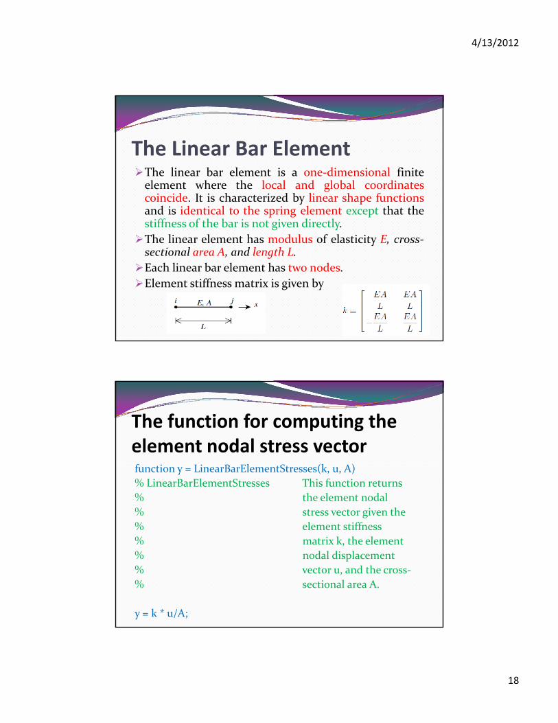
The Linear Bar ElementThe linear bar element is a one‐dimensional finiteelement where the local and global coordinatescoincide. It is characterized by linear shape functionsand is identical to the spring element except that thestiffness of the bar is not given directly.

The linear element has modulus of elasticity E, cross‐sectional area A, and length L.

Each linear bar element has two nodes.

Element stiffness matrix is given by

The function for computing the element nodal stress vectorfunction y = LinearBarElementStresses(k, u, A)

% LinearBarElementStresses This function returns

% the element nodal

% stress vector given the

% element stiffness

% matrix k, the element ,

% nodal displacement

% vector u, and the cross‐

% sectional area A.

y = k * u/A;

4/13/2012

19

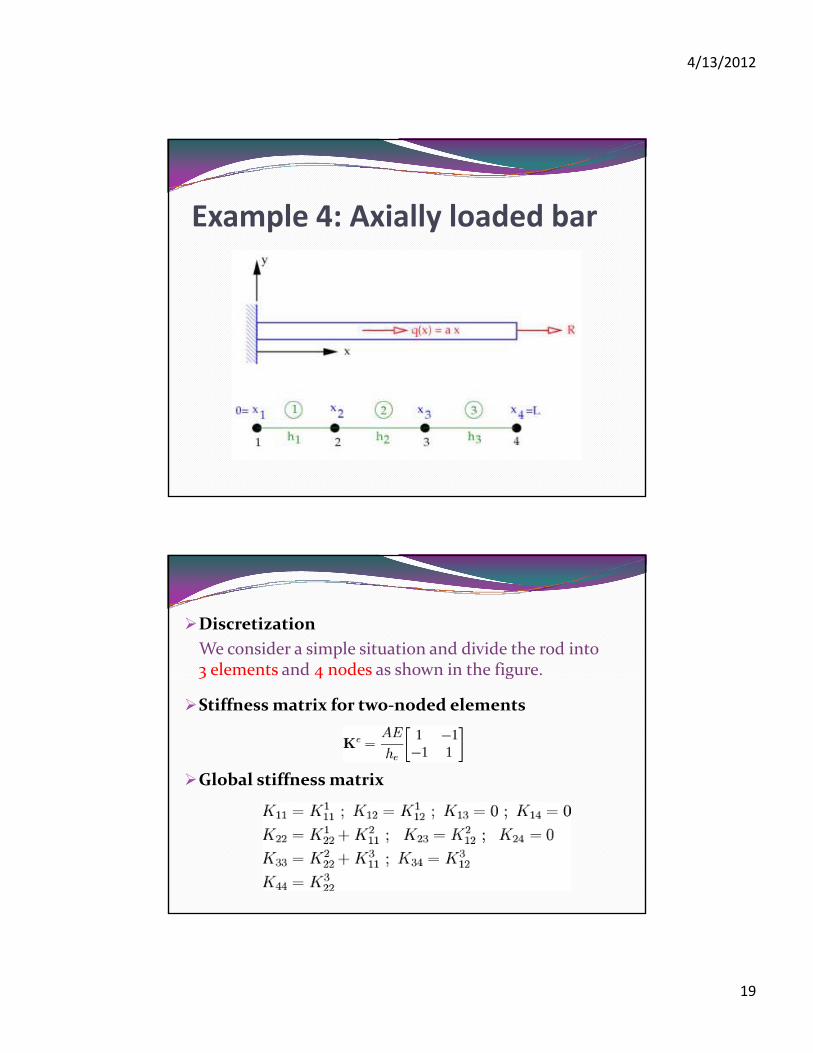
Example 4: Axially loaded bar

Discretization

We consider a simple situation and divide the rod into 3 elements and 4 nodes as shown in the figure.3 elements and 4 nodes as shown in the figure.

Stiffness matrix for two‐noded elements

Global stiffness matrix

4/13/2012

20

Load vector for two‐noded elements

Using the linear shape functions and replacing q withax , the components of the element load vector are

Global load vector

4/13/2012

21

Finite element system of equations

If all the elements are assumed to be of the samelength h, the finite element system of equations canthen be written as

Essential boundary conditions

To solve this system of equations we have to apply theessential boundary condition u=0 at x=0 . This isessential boundary condition u 0 at x 0 . This isequivalent to setting u1 = 0. The reduced system ofequations is

4/13/2012

22

Solve the equationAssume that A, E, L, a, and R are all equal to 1. Then x1 = 0, x2 = 1 / 3, x3 = 2 / 3, x4 = 1, and h = 1 / 3. The system of equations becomes

Computing element strains and stressesThe strain within an element is

The stress in the element is given by

4/13/2012

23

function AxialBarFEMA = 1.0;L = 1.0;E = 1.0;a = 1.0;R = 1 0;

The finite element code (Matlab) usedto compute this solution :

R = 1.0;e = 3;h = L/e;n = e+1;for i=1:nnode(i) = (i‐1)*h;endfor i=1:eelem(i,:) = [i i+1];endK = zeros(n);f eros(n )f = zeros(n,1);for i=1:enode1 = elem(i,1);node2 = elem(i,2);Ke = elementStiffness(A, E, h);fe = elementLoad(node(node1),node(node2), a, h);K(node1:node2,node1:node2) = K(node1:node2,node1:node2) + Ke;f(node1:node2) = f(node1:node2) + fe;end

4/13/2012

24

f(n) = f(n) + 1.0;Kred = K(2:n,2:n);fred = f(2:n);d = inv(Kred)*fred;dsol = [0 d'];fsol = K*dsol';sum(fsol)

figure;p0 = plotDisp(E, A, L, R, a);p1 = plot(node, dsol, 'ro‐‐', 'LineWidth', 3); hold on;legend([p0 p1],'Exact','FEM');for i=1:enode1 = elem(i,1);node2 = elem(i,2);u1 = dsol(node1);u2 = dsol(node2);[eps(i), sig(i)] = elementStrainStress(u1, u2, E, h);End

figure;p0 = plotStress(E, A, L, R, a);for i=1:enode1 = node(elem(i,1));node2 = node(elem(i,2));p1 = plot([node1 node2], [sig(i) sig(i)], 'r‐','LineWidth',3); holdon;Endlegend([p0 p1],'Exact','FEM');

function [p] = plotDisp(E, A, L, R, a)dx = 0.01;nseg = L/dx;for i=1:nseg+1x(i) = (i‐1)*dx;u(i) = (1/6*A*E)*(‐a*x(i)^3 + (6*R + 3*a*L^2)*x(i));

dendp = plot(x, u, 'LineWidth', 3); hold on;xlabel('x', 'FontName', 'palatino', 'FontSize', 18);ylabel('u(x)', 'FontName', 'palatino', 'FontSize', 18);set(gca, 'LineWidth', 3, 'FontName', 'palatino', 'FontSize', 18);

function [p] = plotStress(E, A, L, R, a)dx = 0.01;nseg = L/dx;for i=1:nseg+1for i=1:nseg+1x(i) = (i‐1)*dx;sig(i) = (1/2*A*E)*(‐a*x(i)^2 + (2*R + a*L^2));Endp = plot(x, sig, 'LineWidth', 3); hold on;xlabel('x', 'FontName', 'palatino', 'FontSize', 18);ylabel('\sigma(x)', 'FontName', 'palatino', 'FontSize', 18);set(gca, 'LineWidth', 3, 'FontName', 'palatino', 'FontSize', 18);

4/13/2012

25

function [Ke] = elementStiffness(A, E, h)Ke = (A*E/h)*[[1 ‐1];[‐1 1]];

function [fe] = elementLoad(node1, node2, a, h)x1 = node1;x2 = node2;fe1 = a*x2/(2*h)*(x2^2‐x1^2) ‐ a/(3*h)*(x2^3‐x1^3);fe2 = ‐a*x1/(2*h)*(x2^2‐x1^2) + a/(3*h)*(x2^3‐x1^3);fe = [fe1;fe2];

function [eps, sig] = elementStrainStress(u1, u2, E, h)B = [‐1/h 1/h];u = [u1; u2];eps = B*usig = E*eps;

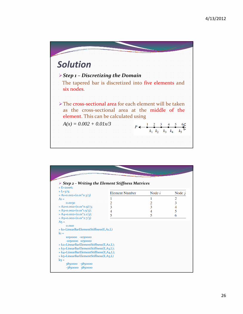
Example 5Consider the tapered bar shown in the figure withp gE = 210GPa and P = 18kN. The cross‐sectional areasof the bar at the left and right ends are 0.002 m²and 0.012 m², respectively. Use linear bar elementsto determine the displacement at the free end ofthe bar.

4/13/2012

26

SolutionStep 1 – Discretizing the DomainStep 1 Discretizing the Domain

The tapered bar is discretized into five elements andsix nodes.

The cross‐sectional area for each element will be takenas the cross‐sectional area at the middle of theelement. This can be calculated using

A(x) = 0.002 + 0.01x/3

Step 2 –Writing the Element Stiffness Matrices» E=210e6;» L=3/5;» A1=0.002+(0.01*0.3/3)A1 =

0.0030» A2=0.002+(0.01*0.9)/3;» A3=0.002+(0.01*1.5/3);» A4=0.002+(0.01*2.1/3);» A5=0.002+(0.01*2.7/3)A5 =

0.0110» k1=LinearBarElementStiffness(E,A1,L)k1 =

1050000 10500001050000 ‐1050000‐1050000 1050000

» k2=LinearBarElementStiffness(E,A2,L);» k3=LinearBarElementStiffness(E,A3,L);» k4=LinearBarElementStiffness(E,A4,L);» k5=LinearBarElementStiffness(E,A5,L)k5 =

3850000 ‐3850000‐3850000 3850000

4/13/2012

27

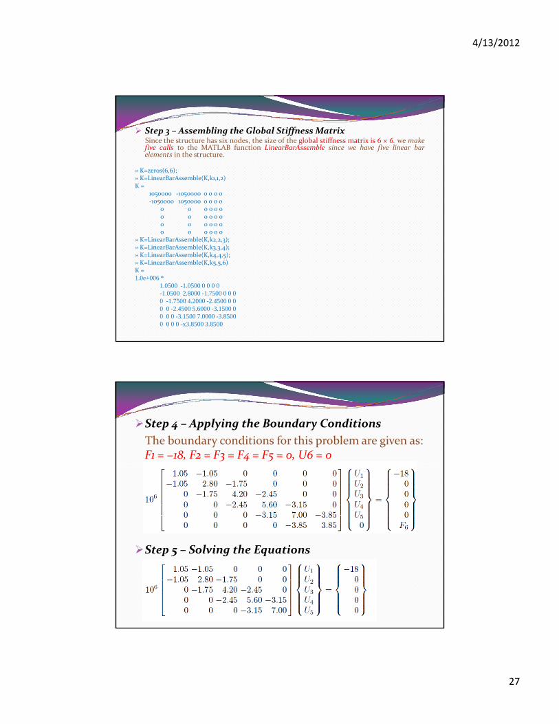
Step 3 – Assembling the Global Stiffness MatrixSince the structure has six nodes, the size of the global stiffness matrix is 6 × 6. we makefive calls to the MATLAB function LinearBarAssemble since we have five linear barelements in the structure.

» K=zeros(6,6);» K LinearBarAssemble(K k1 1 2)» K=LinearBarAssemble(K,k1,1,2)K =

1050000 ‐1050000 0 0 0 0‐1050000 1050000 0 0 0 0

0 0 0 0 0 00 0 0 0 0 00 0 0 0 0 00 0 0 0 0 0

» K=LinearBarAssemble(K,k2,2,3);» K=LinearBarAssemble(K,k3,3,4);» K=LinearBarAssemble(K,k4,4,5);

( )» K=LinearBarAssemble(K,k5,5,6)K =1.0e+006 *

1.0500 -1.0500 0 0 0 0-1.0500 2.8000 -1.7500 0 0 00 -1.7500 4.2000 -2.4500 0 00 0 -2.4500 5.6000 -3.1500 00 0 0 -3.1500 7.0000 -3.85000 0 0 0 -x3.8500 3.8500


The boundary conditions for this problem are given as: F1 = −18, F2 = F3 = F4 = F5 = 0, U6 = 0

S S l i h E iStep 5 – Solving the Equations

4/13/2012

28

» k=K(1:5,1:5)k =1.0e+006 *

1.0500 ‐1.0500 0 0 0‐1.0500 2.8000 ‐1.7500 0 00 ‐1 7500 4 2000 ‐2 4500 00 1.7500 4.2000 2.4500 00 0 ‐2.4500 5.6000 ‐3.15000 0 0 ‐3.1500 7.0000

» f=[‐18 ; 0 ; 0 ; 0 ; 0 ]f =

‐180000

» u= k\fu =1.0e‐004 *

‐0.4517‐0.2802‐0.1774‐0.1039‐0.0468

Example 6

4/13/2012

29

%................................................................% MATLAB codes for Finite Element Analysis% problem2.m% antonio ferreira 2008% clear memoryclear all% E; modulus of elasticity% A: area of cross section% L: length of barE = 30e6;A=1;EA=E*A; L = 90;% generation of coordinates and connectivities% numberElements: number of elementsnumberElements=3;% generation equal spaced coordinatesnodeCoordinates linspace(0 L numberElements+1);nodeCoordinates=linspace(0,L,numberElements+1);xx=nodeCoordinates;% numberNodes: number of nodesnumberNodes=size(nodeCoordinates,2);% elementNodes: connections at elementsii=1:numberElements;elementNodes(:,1)=ii;elementNodes(:,2)=ii+1;

% for structure:% displacements: displacement vector% force : force vector% stiffness: stiffness matrixdisplacements=zeros(numberNodes,1);force=zeros(numberNodes,1);stiffness=zeros(numberNodes,numberNodes);% applied load at node 2force(2)=3000.0;% computation of the system stiffness matrixfor e=1:numberElements;% elementDof: element degrees of freedom (Dof)elementDof=elementNodes(e,:) ;

l th( l tD f)nn=length(elementDof);length_element=nodeCoordinates(elementDof(2))...‐nodeCoordinates(elementDof(1));detJacobian=length_element/2;invJacobian=1/detJacobian;% central Gauss point (xi=0, weight W=2)[shape,naturalDerivatives]=shapeFunctionL2(0.0);Xderivatives=naturalDerivatives*invJacobian;

4/13/2012

30

% B matrixB=zeros(1,nn); B(1:nn) = Xderivatives(:);stiffness(elementDof,elementDof)=...stiffness(elementDof,elementDof)+B’*B*2*detJacobian*EA;( , ) J ;End% boundary conditions and solution% prescribed dofsfixedDof=find(xx==min(nodeCoordinates(:)) ...| xx==max(nodeCoordinates(:)))’;prescribedDof=[fixedDof]% free Dof : activeDofactiveDof=setdiff([1:numberNodes]’,[prescribedDof]);% l i% solutionGDof=numberNodes;displacements=solution(GDof,prescribedDof,stiffness,force);% output displacements/reactionsoutputDisplacementsReactions(displacements,stiffness,...numberNodes,prescribedDof)

% .............................................................function [shape,naturalDerivatives]=shapeFunctionL2(xi)% shape function and derivatives for L2 elements% shape : Shape functions% naturalDerivatives: derivatives w.r.t. xi% naturalDerivatives: derivatives w.r.t. xi% xi: natural coordinates (‐1 ... +1)shape=([1‐xi,1+xi]/2)’;naturalDerivatives=[‐1;1]/2;end % end function shapeFunctionL2

%................................................................function displacements=solution(GDof,prescribedDof,stiffness,f )force)% function to find solution in terms of global displacementsactiveDof=setdiff([1:GDof]’, [prescribedDof]);U=stiffness(activeDof,activeDof)\force(activeDof);displacements=zeros(GDof,1);displacements(activeDof)=U;

Step 4 – Applying the Boundary Conditions The global system of equations :The global system of...

Documents

Transcript of Step 4 – Applying the Boundary Conditions The global system of equations :The global system of...