TIME STEP RESTRICTIONS USING SEMI-IMPLICIT

METHODS FOR THE INCOMPRESSIBLE

NAVIER-STOKES EQUATIONS

WENDY KRESS, PER LOTSTEDT

Dept. of Information Technology, Scientific Computing, Uppsala University, Box 337,SE-75105 Uppsala, Sweden.

Abstract

The incompressible Navier-Stokes equations are discretized in spaceand integrated in time by the method of lines and a semi-implicit method.In each time step a set of systems of linear equations has to be solved.The size of the time steps are restricted by stability and accuracy of thetime-stepping scheme, and convergence of the iterative methods for thesolution of the systems of equations. The stability is investigated with alinear model equation derived from the Navier-Stokes equations. The res-olution in space and time is estimated from turbulent flow physics. Theconvergence of the iterative solvers is studied using the same model equa-tion. The stability constraints and the convergence rate obtained from themodel equation are compared to results for a semi-implicit integrator of theNavier-Stokes equations with good agreement. The most restrictive boundon the time step is given by accuracy, stability, or convergence dependingon the flow conditions and the numerical method.

Keywords: incompressible flow, iterative solution, semi-implicit method,accuracy constraints, stability

AMS subject classification 2000: 65M06, 65M12

1 Introduction

Direct simulation of the Navier-Stokes equations (DNS) is a computational tool tostudy turbulent flow. Spectral and pseudospectral methods have been developedfor this purpose but they are restricted to simple geometries such as straightchannels. For more complex problems a finite difference or finite element methodis more suitable. Examples of such methods are found, e.g., in [4], [6], [27].DNS calculations are computationally very demanding with long execution timesand large memory requirements. One important issue is how the equations are

1

discretized in space. Another question is how to integrate the equations in time.Given the space discretization, the time derivatives are usually approximated bya standard method for ordinary differential equations [18] or a combination ofsuch methods. The scheme may be implicit [11, 34], semi-implicit [6, 20, 34], orexplicit [12, 33]. Then in each time step there are in general one or more systemsof linear equations to solve for the velocity and the pressure. Preferably thesystems of equations are solved by iterative methods since they are superior inefficiency and memory requirements for large problems. In this solution strategy,the time step shall be chosen so that

1. the integration is stable,

2. the solution is sufficiently accurate in time,

3. the iterative solvers converge quickly.

Less computational work is spent in a time interval if the time steps are long, butlong time steps may be in conflict with all three requirements above. Ideally thesolution algorithm should be such that only accuracy restricts the time step butthis is seldom possible for nonlinear problems. In this paper we investigate thismatter and derive bounds on the time step imposed by the stability, accuracy,and convergence for semi-implicit methods in general and the integration methodin [6] in particular.

The Navier-Stokes equations for incompressible flow in two dimensions (2D) inthe primitive variables are as follows. Let u and v be the velocity components inthe x- and y-directions, respectively, p the pressure, and ν the kinematic viscosity.The Reynolds number is defined by Re = ub`/ν for some characteristic velocityub and length scale `. Let w = (u, v)T . Introduce the nonlinear and linear terms

N (w) = (w · ∇)w , L(w, p) = ∇p−Re−1∆w .

Then the Navier-Stokes equations in 2D are

∂tw +N (w) + L(w, p) = 0 , (1)

∇ ·w = 0 . (2)

The space discretizations of N and L in (1) and ∇· in (2) are denoted by Nh

and Lh and ∇h·. Suppose that the solution in space wn is known at time tn andthat we intend to compute wn+1 at tn+1 with the time step ∆t = tn+1 − tn. Inan implicit method, wn+1 fulfills

wn+1 + c1∆tNh(wn+1) + c2∆tLh(w

n+1, p) = bnimpl , (3)

where c1 and c2 are constants depending on the method and bnimpl depends on

previous solutions wn,wn−1 , . . .. The nonlinear term is treated explicitly in asemi-implicit method to avoid the nonlinear equations in (3),

wn+1 + c1∆tLh(wn+1, p) = bn

simpl , (4)

2

where bnsimpl includes Nh and depends on wn,wn−1, . . .. In an explicit scheme,

also the linear term is evaluated from previous solutions,

wn+1 = bnexpl , (5)

so that wn+1 is updated without the need to solve a system of equations for thevelocity.

There are different options to satisfy the incompressibility condition (2) and todetermine the pressure p at tn+1. One possibility is to compute a provisional w∗

and then add a correction so that (2) is satisfied in a pressure correction methodor a projection method [3, 5, 12, 14, 33, 37]. An approximate factorization isdetermined in a fractional step method to obtain two simpler systems of equations[10, 13, 21, 30]. Another way is to solve (3) or (4) and (2) for wn+1 and psimultaneously and iterate until convergence as in [6, 15, 35].

The stability and accuracy of semi-implicit (or mixed explicit/implicit) inte-gration methods for the incompressible Navier-Stokes equations are investigatedin [20]. The length of the time steps is studied in [11] for turbulent flow withan implicit treatment of Nh and Lh. A discussion of appropriate time steps foraccuracy and stability in turbulent flow is found in [16].

The integration method in [6, 7, 28] is semi-implicit as in (4) and second orderaccurate with a fourth order accurate compact finite difference discretization ofthe space derivatives in 2D [8, 22]. The solution is expanded in a Fourier seriesin the third dimension [7]. The system of linear equations for wn+1 and p in eachtime step is solved in one outer and two inner iterations. The analysis developedhere is applied to this method as an example.

The time and space discretizations are discussed in Sect. 2. The time deriva-tive is approximated either by a backward differentiation formula (BDF) or anAdams method. The nonlinear convection term is extrapolated from old solu-tions or advanced by an explicit Adams method. The analysis of the stabilityof the discretization in 2D is based on the Oseen equations with frozen velocitycoefficients in the nonlinear term Nh in Sect. 3. Stability of the particular semi-implicit scheme in [6] is studied in [17] using Fourier analysis. This analysis isgeneralized here to other classes of semi-implicit methods. The model for thestability analysis is validated by comparison of the predictions with the resultsfrom calculations with the Navier-Stokes solver [6] in a straight channel. Themethodology is easily applicable to other space discretizations. The maximumlengths of the temporal and spatial steps for sufficient accuracy are estimated inSect. 4. The assumption is that the scales in time and space in turbulent flowmust be resolved by a certain number of discrete points depending on the orderof accuracy of the discretization. The scales are estimated from basic physicalrelations at the solid wall. The convergence rate and the work in the separatestages of the iterative solution is estimated in Sect. 5. The results of this modelare also corroborated with the iterative solver in [6]. Conclusions are drawn inthe final section.

3

α0 α1 α2 α3 α4 βe1 βe

2 βe3 βe

4

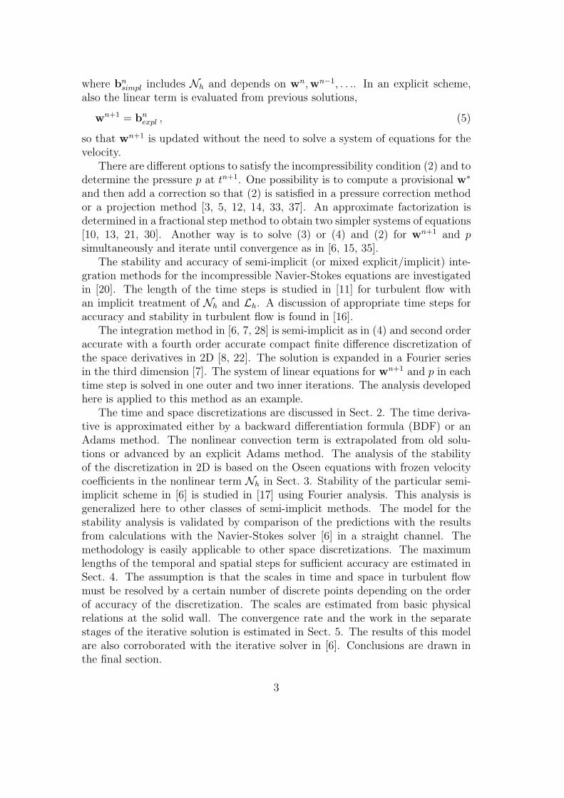
BDF1 1 -1 1BDF2 3/2 -2 1/2 2 -1BDF3 11/6 -3 3/2 -1/3 3 -3 1BDF4 25/12 -4 3 -4/3 1/4 4 -6 4 -1

Table 1: Coefficients for BDF methods (6)

2 Discretization

Equation (1) is discretized in time either by an implicit method (3), a semi-implicit method (4) or an explicit method (5). These methods are here describedfor members of two classes of linear multistep methods: Adams methods andbackward differentiation formulas (BDF) [18]. Linear multistep methods havethe advantage compared to Runge-Kutta (RK) methods that fewer evaluationsof the expensive space derivatives per time step are required.

An implicit scheme is obtained if a BDF-scheme or an implicit Adams-Moultonscheme is applied to (1). The velocity and pressure vectors satisfy a nonlinearsystem of equations (3) and a discretization of (2) in each time step.

One family of semi-implicit methods of order r is obtained by extrapolatingNh(w) from time tn−r+1 up to tn with an (r− 1)-th order polynomial to tn+1 andapplying the r-th order backward differentiation formula (BDFr) to the linearterms to arrive at

r∑j=0

αjwn+1−j + ∆tβi

0Lh(wn+1, pn+1) = −∆t

r∑j=1

βejNh(w

n+1−j) . (6)

The coefficients αj are given by BDFr and the coefficients βej are defined by the

extrapolation

wn+1 =r∑

j=1

βejw

n+1−j +O(∆tr),

and βi0 = 1. The coefficients in (6) up to order r = 4 are given in Table 1. In

addition, wn+1 and p are such that wn+1 satisfies a discretization of the divergenceequation in (2). The result is a system of linear equations for wn+1 and pn+1.The integration is started at t0 with r = 1.

Another class of time discretizations, based on Adams methods, is derivedfrom integrating (1) in time

wn+1 −wn = −∫ tn+1

tnLh(w, p) dt−

∫ tn+1

tnNh(w) dt. (7)

The integral with the nonlinearity is approximated by an explicit Adams-Bashforthmethod and the integral with the linear integrand by an implicit Adams-Moulton

4

βi0 βi

1 βi2 βi

3 βe1 βe

2 βe3 βe

4

Adams2 1/2 1/2 3/2 -1/2Adams3 5/12 8/12 -1/12 23/12 -16/12 5/12Adams4 9/24 19/24 -5/24 1/24 55/24 59/24 37/24 -9/24

Table 2: Coefficients for Adams methods (8)

method [18]. The resulting formula of order r is

wn+1 −wn = −∆t

r−1∑j=0

βijLh(w

n+1−j, pn+1−j)−∆t

r∑j=1

βejNh(w

n+1−j), (8)

i.e., α0 = 1 and α1 = −1. The coefficients for 2 ≤ r ≤ 4 are given in Table2. A common combination is the Adams-Bashforth method of second order andthe implicit trapezoidal (or Crank-Nicolson) method [21, 25]. The last integralin (7) is easily evaluated by an explicit RK scheme at the expense of additionalcalculations of Nh at interior stages between tn and tn+1. The Crank-Nicolsonscheme is combined with an explicit RK method in [4] and a more elaborate RKmethod in [24].

u

v

p

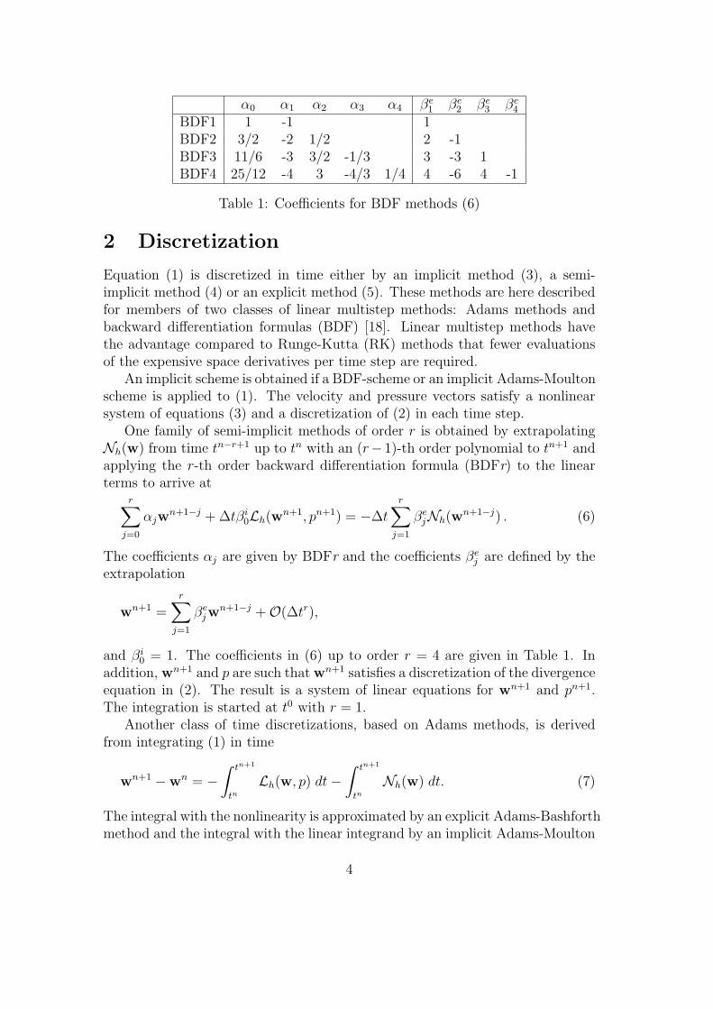
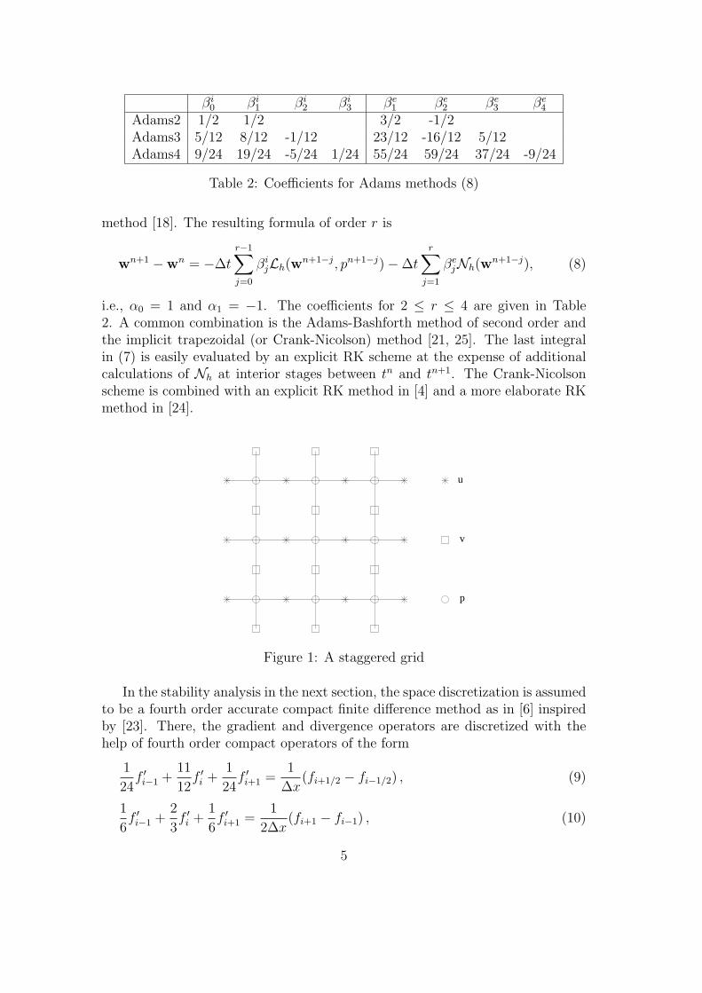
Figure 1: A staggered grid

In the stability analysis in the next section, the space discretization is assumedto be a fourth order accurate compact finite difference method as in [6] inspiredby [23]. There, the gradient and divergence operators are discretized with thehelp of fourth order compact operators of the form

1

24f ′i−1 +

11

12f ′i +

1

24f ′i+1 =

1

∆x(fi+1/2 − fi−1/2) , (9)

1

6f ′i−1 +

2

3f ′i +

1

6f ′i+1 =

1

2∆x(fi+1 − fi−1) , (10)

5

and for the Laplacian, formulas of the type

1

12f ′′i−1 +

10

12f ′′i +

1

12f ′′i+1 =

1

∆x2(fi−1 − 2fi + fi+1) (11)

are used on a Cartesian grid. Together with appropriate numerical boundaryconditions, equations (9), (10) and (11) can be written in matrix form as Pf ′ =Qf , P f ′ = Qf and Rf ′′ = Sf , respectively. The components u, v, and p arecalculated at different points on a staggered grid, as depicted in Figure 1. On aCartesian grid, the fourth order discretization becomes

Lh(w, p) =

(P−1

x Qxp−Re−1(R−1x Sx + R−1

y Sy)uP−1

y Qyp−Re−1(R−1x Sx + R−1

y Sy)v

),

Nh(w) =

(uP−1

x Qxu + EvP−1y Qyu

EuP−1x Qxv + vP−1

y Qyv

),

∇h ·w = P−1x Qxu + P−1

y Qyv ,

(12)

where E is an interpolation operator between the u and v points, see [8]. Astandard second order discretization is achieved by replacing P , P and R withidentity operators.

3 Stability analysis

The Navier-Stokes equations are linearized by freezing the velocity w in front ofthe gradient in the nonlinear term to obtain the Oseen equations as in [17]

wt + (w · ∇)w + L(w, p) = 0 , (13)

∇ ·w = 0 . (14)

where w = (u, v) consists of two constants. A rectangular physical domain withperiodic boundary conditions is discretized with a Cartesian grid with constantstep sizes ∆x and ∆y. The space discretization (12) and a Fourier transformationin x and y is used to arrive at a system of equations for the transformed variablesw = (u, v)T and p. Let ω1 and ω2 be the discrete wavenumbers in the x and ydirections and introduce the notation

ξ1 = ω1∆x , ξ2 = ω2∆y , 0 ≤ |ξ1|, |ξ2| ≤ π ,λx = ∆t/∆x , λy = ∆t/∆y , sj = sin ξj/2 , cj = cos ξj/2, j = 1, 2 .

The CFL-numbers in the x- and y-directions are uλx and vλy. For the Fouriertransformation of the equations of fourth order accuracy the following coefficients

6

are introduced,

a1 =3i sin ξ1

2 + cos ξ1

=6is1c1

1 + 2c21

, a2 =3i sin ξ2

2 + cos ξ2

=6is2c2

1 + 2c22

, (15a)

b1 =24is1

11 + cos ξ1

=12is1

5 + c21

, b2 =24is2

11 + cos ξ2

=12is2

5 + c22

, (15b)

c0 = 24

(s21

5 + cos ξ1

+∆x2s2

2

∆y2(5 + cos ξ2)

)= 12

(s21

2 + c21

+∆x2s2

2

∆y2(2 + c22)

),

(15c)

θ =∆t

Re∆x2. (15d)

The standard, centered second order accurate space discretization generates thefollowing coefficients

a1 = 2is1c1 , a2 = 2is2c2 , (16a)

b1 = 2is1 , b2 = 2is2 , (16b)

c0 = 4(s21 + ∆x2s2

2/∆y2)

. (16c)

Then the Fourier transformed system for the variables u, v and p isr∑

j=0

αjun+1−j + (uλxa1 + vλya2)

r∑j=1

βej u

n+1−j

+λxb1

r−1∑j=0

βij p

n+1−j + θc0

r−1∑j=0

βiju

n+1−j = 0, (17a)

r∑j=0

αj vn+1−j + (uλxa1 + vλya2)

r∑j=1

βej v

n+1−j

+λyb2

r−1∑j=0

βij p

n+1−j + θc0

r−1∑j=0

βij v

n+1−j = 0, (17b)

b1un+1 + b2v

n+1 = 0 . (17c)

Multiply (17a) by b1 and (17b) by b2 and add them together. Since (17c) issatisfied by un and vn for all n ≥ 1, the equation for pn+1 is

(λxb21 + λyb

22)

r−1∑j=0

βij p

n+1−j = 0. (18)

If at least one ξj, j = 1, 2, satisfies ξj 6= 0, then λxb21 + λyb

22 6= 0 and the sum in

(18) vanishes. Then (17b) for vn+1 is identical to (17a) for un+1. We can rewritethe first equation with βi

r = 0 to obtain

(α0 + βi0θc0)u

n+1 +r∑

j=1

(αj + βej (uλxa1 + vλya2) + βi

jθc0)un+1−j = 0.

7

For ξ1 = ξ2 = 0 the time-integration degenerates to

r∑j=0

αjun+1−j = 0. (19)

BDF methods are zero-stable for 1 ≤ r ≤ 6 and all Adams methods have thisproperty [18] and therefore the sequence un in (19) is stable for such r.

We can show that there is no parasitic odd-even oscillatory solution for thesecond and fourth order approximations, cf. [17]. Consider the steady state casein (17). The equations are the same for u and v. We can assume the scaling∑r

j=1 βej =

∑r−1j=0 βi

j = 1. Since∑r

j=0 αj = 0, the time-independent u fulfills

(θc0 + uλxa1 + vλya2)u = 0.

With ξ1 = ξ2 = π in (15) and (16) corresponding to the odd-even parasiticsolution, the equation is

θc0u = 0,

showing that no non-trivial solution exists.The stability of the scheme when ξ1 and ξ2 are not both zero is determined

by the roots of the polynomial

(α0 + βi0θc0)z

r +r∑

j=1

(αj + βej (uλxa1 + vλya2) + βi

jθc0)zr−j = 0. (20)

The scheme is stable if all roots z of the characteristic equation (20) satisfy |z| ≤ 1and if |z| = 1 then it is a simple root.

3.1 Stability domain for BDF2

Let ϑ = θc0. The characteristic equation for the second order BDF method, r = 2in Table 1, is then given by

(1.5 + ϑ)z2 + 2(ξ − 1)z + (0.5− ξ) = 0 , (21)

where we have introduced ξ = uλxa1 + vλya2. The boundary of the stabilitydomain is determined by calculating the values of ξ for |z| = 1. The method isstable for values of ξ inside the boundary. In addition, ξ is purely imaginary.Thus, we only consider an interval on the imaginary axis.

Proposition 1. The characteristic equation (21) has stable solutions |z| ≤ 1for ξ in the interval [−ξ∗, ξ∗], where

ξ∗ = i

√3ϑ(1 + ϑ)(2 + ϑ)− ϑ(1 + ϑ)√2(3 + ϑ)

√3ϑ(1 + ϑ) + 3ϑ

.

8

Proof

With ξ∗ purely imaginary, equation (21) together with |z| = 1 leads to threeequations for the real and imaginary parts of z, <(z) and =(z), and =(ξ∗):

(1.5 + ϑ)(<(z)2 −=(z)2)− 2(=(ξ∗)=(z) + <(z)) + 0.5 = 0 ,(1.5 + ϑ)2<(z)=(z) + 2(=(ξ∗)<(z)−=(z))−=(ξ∗) = 0 ,

<(z)2 + =(z)2 = 1 .

(22)

Taking into account symmetry, we consider only =(ξ∗) ≥ 0. The solution to (22)is given by

<(z) =3 + ϑ−

√3ϑ(1 + ϑ)

3 + 2ϑ,

=(z) =

√2(3 + ϑ)

√3ϑ(1 + ϑ) + 3ϑ

3 + 2ϑ,

=(ξ∗) =

√3ϑ(1 + ϑ)(2 + ϑ)− ϑ(1 + ϑ)√2(3 + ϑ)

√3ϑ(1 + ϑ) + 3ϑ

.

(23)

Only z = 0.5 is a double root.For fixed θ, the boundary of the stability domain in the uλx–vλy plane is

calculated by

uλx = minω1,ω2

(−vλya2/a1 + ξ∗/a1) .

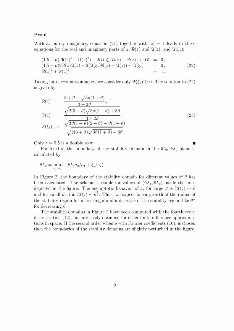
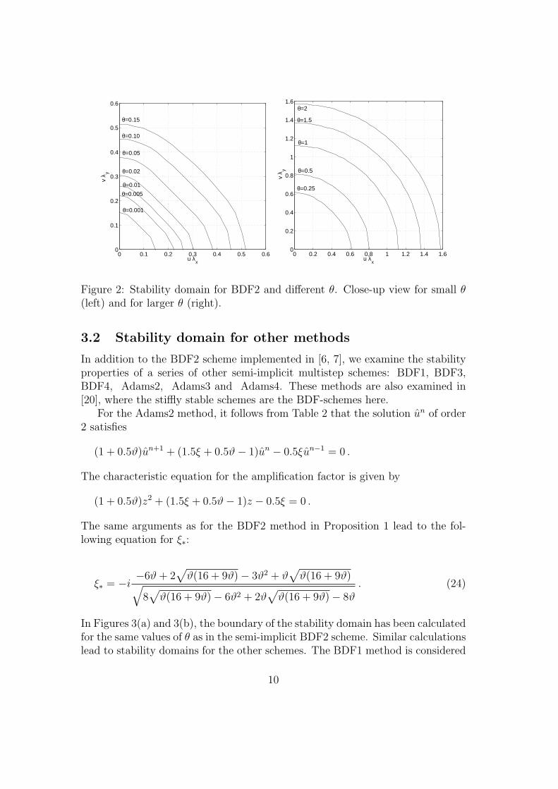
In Figure 2, the boundary of the stability domain for different values of θ hasbeen calculated. The scheme is stable for values of (uλx, vλy) inside the linesdepicted in the figure. The asymptotic behavior of ξ∗ for large ϑ is =(ξ∗) ∼ ϑ

and for small ϑ, it is =(ξ∗) ∼ ϑ14 . Thus, we expect linear growth of the radius of

the stability region for increasing θ and a decrease of the stability region like θ14

for decreasing θ.The stability domains in Figure 2 have been computed with the fourth order

discretization (12), but are easily obtained for other finite difference approxima-tions in space. If the second order scheme with Fourier coefficients (16), is chosenthen the boundaries of the stability domains are slightly perturbed in the figure.

9

0 0.1 0.2 0.3 0.4 0.5 0.60

0.1

0.2

0.3

0.4

0.5

0.6

u λx

v λ y

θ=0.15

θ=0.10

θ=0.05

θ=0.02

θ=0.01

θ=0.005

θ=0.001

0 0.2 0.4 0.6 0.8 1 1.2 1.4 1.60

0.2

0.4

0.6

0.8

1

1.2

1.4

1.6

u λx

v λ y

θ=2

θ=1.5

θ=1

θ=0.5

θ=0.25

Figure 2: Stability domain for BDF2 and different θ. Close-up view for small θ(left) and for larger θ (right).

3.2 Stability domain for other methods

In addition to the BDF2 scheme implemented in [6, 7], we examine the stabilityproperties of a series of other semi-implicit multistep schemes: BDF1, BDF3,BDF4, Adams2, Adams3 and Adams4. These methods are also examined in[20], where the stiffly stable schemes are the BDF-schemes here.

For the Adams2 method, it follows from Table 2 that the solution un of order2 satisfies

(1 + 0.5ϑ)un+1 + (1.5ξ + 0.5ϑ− 1)un − 0.5ξun−1 = 0 .

The characteristic equation for the amplification factor is given by

(1 + 0.5ϑ)z2 + (1.5ξ + 0.5ϑ− 1)z − 0.5ξ = 0 .

The same arguments as for the BDF2 method in Proposition 1 lead to the fol-lowing equation for ξ∗:

ξ∗ = −i−6ϑ + 2

√ϑ(16 + 9ϑ)− 3ϑ2 + ϑ

√ϑ(16 + 9ϑ)√

8√

ϑ(16 + 9ϑ)− 6ϑ2 + 2ϑ√

ϑ(16 + 9ϑ)− 8ϑ. (24)

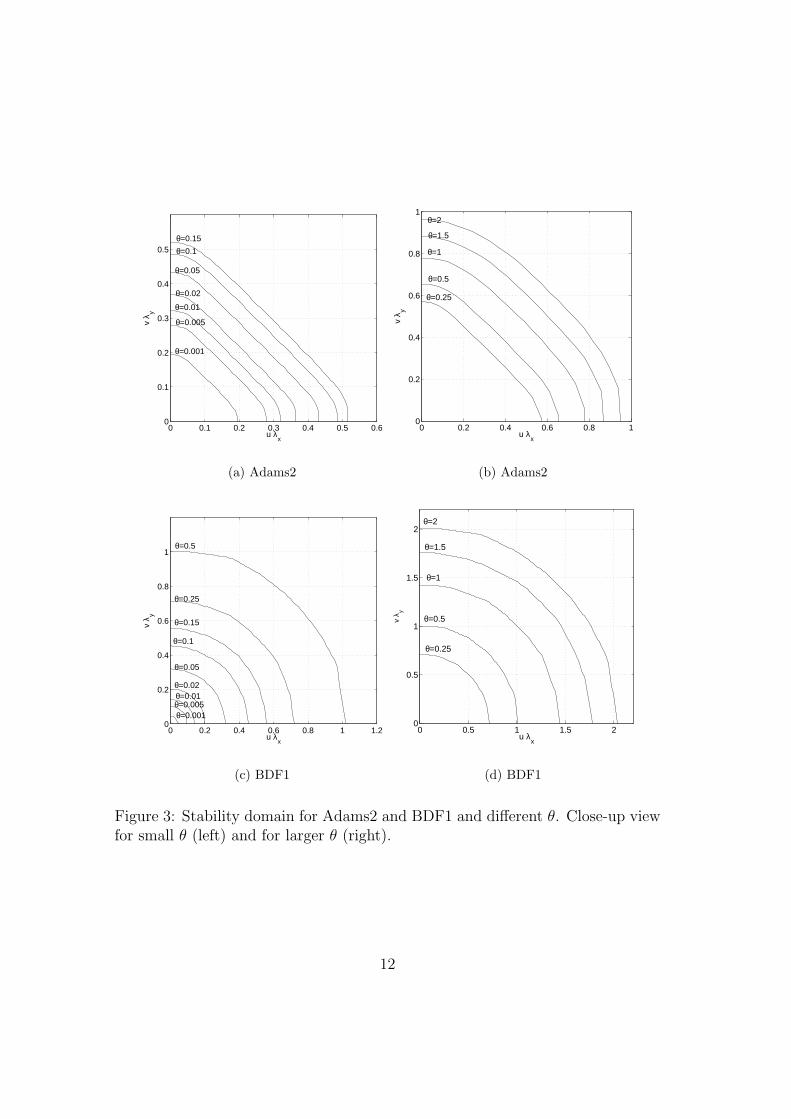
In Figures 3(a) and 3(b), the boundary of the stability domain has been calculatedfor the same values of θ as in the semi-implicit BDF2 scheme. Similar calculationslead to stability domains for the other schemes. The BDF1 method is considered

10

in Figures 3(c) and 3(d). Higher order BDF and Adams methods are consideredin Figures 4 and 5. The methods are stable for points (uλx, vλy) inside thecontours. Closed expressions such as in (23) and (24) are not available for thethird and fourth order methods. The roots of the characteristic equations arecomputed numerically.

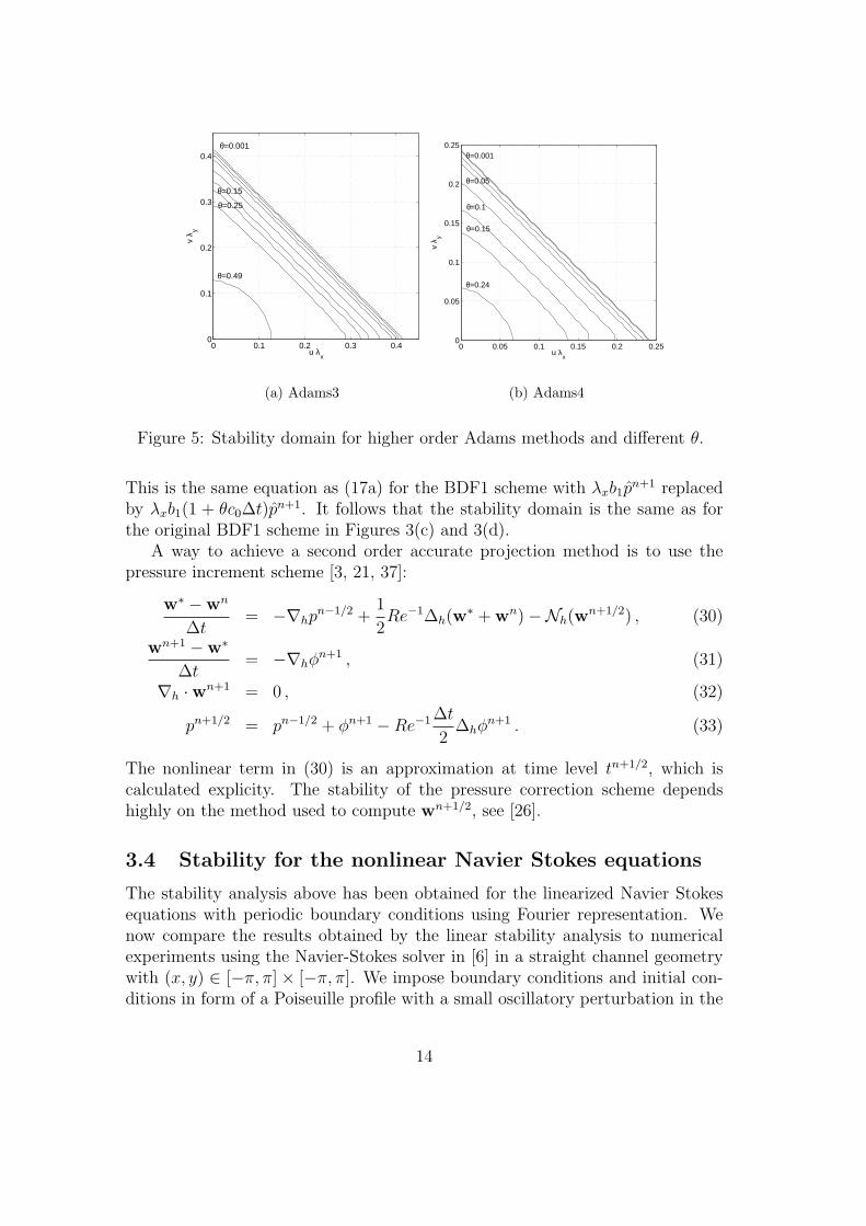
For the higher order BDF schemes, as θ decreases the stability domain ap-proaches the triangles (uλx + vλy) ≤ 0.367 for BDF3 and (uλx + vλy) ≤ 0.313for BDF4. For the Adams methods, the stability domain grows for decreasing θ.Adams3 and Adams4 become unstable for θ > 1

2and θ > 1

4respectively. This is

due to the fact that the stability domain of the higher order implicit Adams meth-ods does not include the entire negative real axis [19]. The stability domains arelimited from above by (uλx + vλy) ≤ 0.416 for Adams3 and (uλx + vλy) ≤ 0.243for Adams4. The Adams3 scheme was deemed ’inappropriate for all practicalreasons’ in [20].

For fully explicit methods, the stability analysis can be simplified and a stan-dard scalar stability analysis as in [19] can be applied.

3.3 Projection methods

In the previous subsection, we have assumed that the equations for un+1, vn+1,and pn+1 are solved simultaneously. Another way of solving the Navier Stokesequations is to decouple the equations for the velocity and the pressure by usingprojection methods. The classical projection method [12, 33] is

w∗ −wn

∆t= Re−1∆hw

∗ −Nh(wn) , (25)

wn+1 −w∗

∆t= −∇hp

n+1 , (26)

∇h ·wn+1 = 0 . (27)

The subscript h denotes the discretized spatial operators introduced in Sect. 2.In practice the equations are solved by taking the discrete divergence of (26)which results in a Poisson equation for the pressure. The scheme is first orderaccurate and can be written as

wn+1 −wn

∆t= −∇hp

n+1 + Re−1∆h(wn+1 + ∆t∇hp

n+1)−Nh(wn) , (28)

∇h ·wn+1 = 0 . (29)

We can now perform a similar analysis as in the beginning of Sect. 3. Fouriertransformation in space yields the following transformed equation for u and thesame equation for v

un+1 − un + (uλxa1 + vλya2)un + λxb1(1 + θc0∆t)pn+1 = −θc0u

n+1 .

11

0 0.1 0.2 0.3 0.4 0.5 0.60

0.1

0.2

0.3

0.4

0.5

u λx

v λ y

θ=0.15

θ=0.1

θ=0.05

θ=0.02

θ=0.01

θ=0.005

θ=0.001

(a) Adams2

0 0.2 0.4 0.6 0.8 10

0.2

0.4

0.6

0.8

1

u λx

v λ y

θ=2

θ=1.5

θ=1

θ=0.5

θ=0.25

(b) Adams2

0 0.2 0.4 0.6 0.8 1 1.20

0.2

0.4

0.6

0.8

1

u λx

v λ y

θ=0.001θ=0.005θ=0.01θ=0.02

θ=0.05

θ=0.1

θ=0.15

θ=0.25

θ=0.5

(c) BDF1

0 0.5 1 1.5 20

0.5

1

1.5

2

u λx

v λ y

θ=0.25

θ=0.5

θ=1

θ=1.5

θ=2

(d) BDF1

Figure 3: Stability domain for Adams2 and BDF1 and different θ. Close-up viewfor small θ (left) and for larger θ (right).

12

0 0.1 0.2 0.3 0.4 0.5 0.60

0.1

0.2

0.3

0.4

0.5

u λx

v λ x

θ=0.25

θ=0.15

θ=0.001

θ=0.5

(a) BDF3

0 0.2 0.4 0.6 0.8 10

0.2

0.4

0.6

0.8

1

u λx

v λ y

θ=0.25

θ=0.5

θ=1

θ=1.5

θ=2

(b) BDF3

0 0.1 0.2 0.3 0.40

0.1

0.2

0.3

0.4

u λx

v λ y

θ=0.5

θ=0.25

θ=0.001

(c) BDF4

0 0.1 0.2 0.3 0.4 0.5 0.60

0.1

0.2

0.3

0.4

0.5

u λx

v λ y

θ=2

θ=1.5

θ=1

θ=0.5

θ=0.25

(d) BDF4

Figure 4: Stability domain for higher order BDF schemes and different θ. Close-up view for small θ (left) and for larger θ (right).

13

0 0.1 0.2 0.3 0.40

0.1

0.2

0.3

0.4

u λx

v λ y

θ=0.001

θ=0.15

θ=0.25

θ=0.49

(a) Adams3

0 0.05 0.1 0.15 0.2 0.250

0.05

0.1

0.15

0.2

0.25

u λx

v λ y

θ=0.001

θ=0.05

θ=0.1

θ=0.15

θ=0.24

(b) Adams4

Figure 5: Stability domain for higher order Adams methods and different θ.

This is the same equation as (17a) for the BDF1 scheme with λxb1pn+1 replaced

by λxb1(1 + θc0∆t)pn+1. It follows that the stability domain is the same as forthe original BDF1 scheme in Figures 3(c) and 3(d).

A way to achieve a second order accurate projection method is to use thepressure increment scheme [3, 21, 37]:

w∗ −wn

∆t= −∇hp

n−1/2 +1

2Re−1∆h(w

∗ + wn)−Nh(wn+1/2) , (30)

wn+1 −w∗

∆t= −∇hφ

n+1 , (31)

∇h ·wn+1 = 0 , (32)

pn+1/2 = pn−1/2 + φn+1 −Re−1 ∆t

2∆hφ

n+1 . (33)

The nonlinear term in (30) is an approximation at time level tn+1/2, which iscalculated explicity. The stability of the pressure correction scheme dependshighly on the method used to compute wn+1/2, see [26].

3.4 Stability for the nonlinear Navier Stokes equations

The stability analysis above has been obtained for the linearized Navier Stokesequations with periodic boundary conditions using Fourier representation. Wenow compare the results obtained by the linear stability analysis to numericalexperiments using the Navier-Stokes solver in [6] in a straight channel geometrywith (x, y) ∈ [−π, π]× [−π, π]. We impose boundary conditions and initial con-ditions in form of a Poiseuille profile with a small oscillatory perturbation in the

14

0 100 200 300 400 500 600 7000.01

0.02

0.03

0.04

0.05

0.06

0.07

0.08

0.09

Re

∆t *

(a) Nx = 24

0 100 200 300 400 500 600 7000.015

0.02

0.025

0.03

0.035

0.04

0.045

0.05

Re

∆ t *

(b) Nx = 48

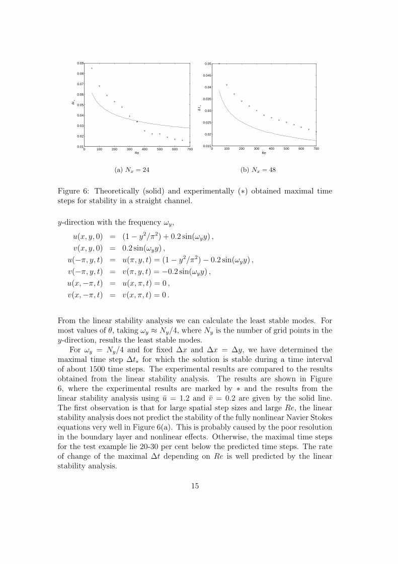
Figure 6: Theoretically (solid) and experimentally (∗) obtained maximal timesteps for stability in a straight channel.

y-direction with the frequency ωy,

u(x, y, 0) = (1− y2/π2) + 0.2 sin(ωyy) ,

v(x, y, 0) = 0.2 sin(ωyy) ,

u(−π, y, t) = u(π, y, t) = (1− y2/π2)− 0.2 sin(ωyy) ,

v(−π, y, t) = v(π, y, t) = −0.2 sin(ωyy) ,

u(x,−π, t) = u(x, π, t) = 0 ,

v(x,−π, t) = v(x, π, t) = 0 .

From the linear stability analysis we can calculate the least stable modes. Formost values of θ, taking ωy ≈ Ny/4, where Ny is the number of grid points in they-direction, results the least stable modes.

For ωy = Ny/4 and for fixed ∆x and ∆x = ∆y, we have determined themaximal time step ∆t∗ for which the solution is stable during a time intervalof about 1500 time steps. The experimental results are compared to the resultsobtained from the linear stability analysis. The results are shown in Figure6, where the experimental results are marked by ∗ and the results from thelinear stability analysis using u = 1.2 and v = 0.2 are given by the solid line.The first observation is that for large spatial step sizes and large Re, the linearstability analysis does not predict the stability of the fully nonlinear Navier Stokesequations very well in Figure 6(a). This is probably caused by the poor resolutionin the boundary layer and nonlinear effects. Otherwise, the maximal time stepsfor the test example lie 20-30 per cent below the predicted time steps. The rateof change of the maximal ∆t depending on Re is well predicted by the linearstability analysis.

15

4 Accuracy

In this section the length and time scales for turbulent flow in a boundary layerare investigated to estimate the spatial step ∆x and the time step ∆t required fora sufficient accuracy in the discretization. The geometry is typically a straightchannel. The assumption is that certain numbers of grid points, nl and nt, areneeded to resolve the length scale and the time scale, respectively. The numbersnl and nt depend on the order of accuracy of the discretization. Then the CFL-number uλx and θ can be estimated.

Let uτ be the friction velocity defined by√

ν∂u/∂y at a wall with y increasingin the normal direction. In near-wall turbulence the length scale `w is y+ =uτ`w/ν = 1, [16, 38], i.e. `w = ν/uτ , and the time scale is tw = `w/uτ = ν/u2

τ .Introduce the quotient χ = ub/uτ between the base flow velocity and the frictionvelocity. In dimensionless quantities the scales Lw and Tw at the solid wall arenow

Lw =`w

`=

ν

uτ`=

χ

Re, Tw =

twub

`=

νub

u2τ`

=χ2

Re. (34)

Assume that we need nt time steps ∆t to resolve the time scale and nl spacesteps ∆x to resolve the length scale. Then at the wall

∆xw =Lw

nl

=χ

nlRe, ∆tw =

Tw

nt

=χ2

ntRe= χ

nl

nt

∆xw. (35)

The quotient χ varies slowly with Re. In DNS experiments in a channel in[1] χ is about 15 in a case with Re = 1955 and increases to 17 when Re = 6210.The measured data in a channel in [29] show a growth in χ from 25 to 31 whenRe increases from 5000 to 30000. In turbulent pipe flow at Re = 5317 in [16]χ = 15. The friction coefficient cf is defined by

cf = u2τ/(0.5u

2b) = 2χ−2

for turbulent flow over a flat plate with Re > 105. It satisfies the empiricalrelation

cf = 0.0576ubν−1x−1/5,

where x is the position in the downstream direction on the plate [32]. Combiningthe two expressions for cf the result for χ is

χ = 5.9Re0.1(x/`)0.1,

which is about 19 for Re = 105 and x = `. Hence, by (35) usually ∆tw > ∆xw.

16

It follows that at the wall

uλw =uτ

ub

λw = χ−1 ∆tw∆xw

= χ−1 Twnl

Lwnt

=nl

nt

,

θw =∆tw

Re∆x2w

=n2

l

nt

.(36)

For good accuracy in time and space with a second order method in time and afourth order method in space we need, say, nt = 10 and nl = 4, see [23]. Hence,u∆tw/∆xw = 0.4. In [11], the time steps are found in numerical experiments ina plane channel to be such that nt ≈ 5 in a second order method similar to theCrank-Nicolson method. The CFL-number for good accuracy is there rather low,0.5− 1.

A much smaller time step is necessary for high accuracy in other flow regimes,such as transitional flow [16].

5 Iterative method

In every time step with a semi-implicit method, a system of linear equationshas to be solved for (wn+1, pn+1) at the N grid points. Let wn+1 ∈ R2N andpn+1 ∈ RN be the solution vectors. Then let Dwn+1 approximate the divergenceof the velocity, Gpn+1 the gradient of the pressure, and Lwn+1 the Laplacianapplied to the velocity components. Here

D ∈ RN×2N , G ∈ R2N×N , L ∈ R2N×2N ,

and A is defined by

A = α0I −Re−1∆tβi0L.

The new solution at tn+1 satisfies(

A ∆tβi0G

D 0

) (wn+1

pn+1

)=

(b1

b2

), (37)

where b1 and b2 depend on previous solutions wn−i, pn−i, i = 0, 1, 2 . . ., and theboundary conditions. The structure of (37) is the same, independent of the timestepping method in Sect. 3.

Two different approaches to solution of (37) are investigated here:

1. An approximate factorization of the system matrix is introduced as in [6,10, 13, 30].

2. An exact factorization of the matrix defines a Schur complement system oflinear equations for the pressure as in [9, 15, 35].

17

An overview and a discussion of different factorizations of the matrix in (37) inthe same spirit as below is found in [31].

In the first case an LU-factorization of a nearby matrix is computed(

A ∆tβi0G

D 0

)≈

(A 0D −α−1

0 ∆tβi0DG

)(I α−1

0 ∆tβi0G

0 I

)

=

(A α−1

0 ∆tβi0AG

D 0

).

(38)

To compute wn+1 and pn+1 with the approximate factorization, two systems oflinear equations have to be solved in a forward and a backward substitution sweep

1. Aw∗ = b1,2. DGpn+1 = α0(∆tβi

0)−1(Dw∗ − b2),

3. wn+1 = w∗ − α−10 βi

0∆tGpn+1.(39)

In [10, 13, 30] these values of wn+1 and pn+1 are accepted but in [6] an outeriteration ensures that (37) is solved with sufficient accuracy.

A pressure correction method and the projection method (26) generate thesame systems of equations to solve as in (39), see Sect. 3.3 and [2, 3, 5, 14, 33, 37].

An exact factorization of the matrix in (37) is(

A ∆tβi0G

D 0

)=

(A 0D −∆tβi

0DA−1G

)(I ∆tβi

0A−1G

0 I

). (40)

In the second alternative, the steps to solve (37) for the velocity and the pressureare

1. Aw∗ = b1,2. DA−1Gpn+1 = (∆tβi

0)−1(Dw∗ − b2),

3. wn+1 = w∗ − βi0∆tA−1Gpn+1.

(41)

The inverse of A is dense and is not computed and stored. In an iterativesolution of step 2 in (41) with a Krylov method where the multiplication of anarbitrary vector f with DA−1G is needed, either A−1 is approximated [15, 35] ora system of equations is solved

Ag = Gf

to compute DA−1Gf = Dg. In step 1, the system is solved by an iterativemethod. The system in step 3 is solved either with an approximation of A−1 orby an iterative method after multiplying the left and right hand sides with A.The approximation of A−1 in step 2 may be different from the one in step 3.

Sufficient accuracy in the solution of (37) is obtained by solving it iterativelyusing the approximate factorization (38) [6] or the exact factorization (40) withan approximation of A−1 [35]. Let the original system (37) be

Mx = b , (42)

18

where x = (wn+1, pn+1)T and b = (bT1 , bT

2 )T , and denote the approximate factor-ization matrix (38) or an approximation of the factorization (40) by M . Then

M =

(A 0D −∆tβi

0DBG

)(I ∆tβi

0BG0 I

), (43)

where B = α−10 I in (38) and B = A−1 or B approximates A−1 in (40).

To solve (42), we use a fixed point iteration with M as a preconditioner in anouter iteration, i.e.

x(k+1) = x(k) + δx(k) = x(k) + M−1(b−Mx(k)) = x(k) + M−1r(k) , (44)

or

r(k+1) = b−Mx(k+1) = (I −MM−1)r(k).

The solution of

Mδx(k) = r(k) (45)

is computed either as in (39) or (41). The difference between M and M in (38)and (40) is in the submatrix M12 in the upper right corner

M12 − M12 = ∆tβi0(I − AB)G,

where

M12 − M12 = α−10 (∆tβi

0)2Re−1LG,

if B = α−10 I as it is in (38). In a fractional step, pressure correction or projection

method a system like (45) is solved once in each time step, corresponding to oneiterative step in (44).

Two systems of equations have to be solved in (39) and (41)

1. Ay1 = b1 , (46)

2. DBGy2 = (∆tβi0)−1(Dy1 − b2) . (47)

The simplest way to solve (46) is by a preconditioned fixed point iteration

y(k+1)1 = y

(k)1 + δy

(k)1 = y

(k)1 + A−1(b1 − Ay

(k)1 ) . (48)

One possible choice of A is α0I. This is also how B−1 can be chosen in (41) [35].Another choice is A = α0I −∆tβi

0Re−1L2 where L2 is a simple approximation ofthe Laplacian.

System (47) is similar to a Poisson equation, but the matrix is not necessarilysymmetric and the matrix may not be explicitly available. This is the case withthe discretization (12).

19

5.1 Convergence of the iterative solvers

It follows from (43) that

I −MM−1 =

(FDA−1 −F

0 0

)

with F = (AB − I)G(DBG)−1. A necessary and sufficient condition for conver-gence of the outer iterations (44), is that the spectral radius of I −MM−1 is lessthan 1, i.e., the eigenvalues of FDA−1 have modulus less than one.

It is proved in [35] under certain conditions on B, e.g. if B = α−10 I as in

(38), that the eigenvalues λi(I − MM−1) of I − MM−1 satisfy |λi| < 1 for allbounded ∆t > 0. This bound is easily determined in two cases showing theexplicit dependence of ∆t.

Proposition 2. Assume that B = α−10 I.

If L is symmetric with non-positive eigenvalues λi(L) and D = GT , then theeigenvalues satisfy

0 ≤ λi(I −MM−1) ≤ γ maxi |λi(L)|α0 + γ maxi |λi(L)| < 1 , (49)

with γ = ∆tβi0Re−1.

If the solution is periodic and discretized with the fourth order operator inSect. 3, then

0 ≤ λi(I −MM−1) ≤ 12βi0θ

α0 + 12βi0θ

< 1 . (50)

Proof

In the first case, let

J = −γL, P = G(GT G)−1GT , K = (α0I − γL)−1.

Then F can be written F = −JG(DG)−1. An eigenvalue λ of FDA−1 fulfills

JPKx = λx. (51)

Since KJ is symmetric and has non-negative eigenvalues, it has a symmetricfactorization KJ = CT C and P is a symmetric projection matrix with P T P = P .Introduce y = CJ−1x in (51) to obtain

(PCT )T PCT y = λy.

20

Hence, λ is non-negative. Since P is a projection matrix we have

maxi λi((PCT )T PCT ) = ‖PCT‖2 ≤ ‖P‖2‖CT‖2 = maxi λi(CT C)

= maxi λi(KJ) = γ maxi |λi(L)|/(α0 + γ maxi |λi(L)|),and (49) is proved.

In the second case, the eigenvalues of FDA−1 are θβi0c0/(α0 + θβi

0c0) with c0

and θ defined in (15c) and (15d). For ∆x = ∆y we have c0 ≤ 12. Thus, (50)follows since α0 is positive.

The spectral radius is less than one for all time steps ∆t in both cases in thetheorem. Hence, under the conditions of the theorem there is no restiction onthe time step introduced by the outer iteration (44).

We now turn to the solution of the inner system. The first inner system (46)is also solved by a fixed point iteration as in (48). For the residual we have

ρ(l+1)1 = b1 − Ay

(l+1)1 = b1 − A(y

(l)1 + A−1(b1 − Ay

(l)1 ))

= (I − AA−1)ρ(l)1 ,

and thus,

‖ρ(l)1 ‖ ≤ ‖I − AA−1‖l‖ρ(0)

1 ‖ .

The fixed point iteration for the first inner system with A−1 = α−10 I converges if

µA = ‖I − AA−1‖ = α−10 ∆tβi

0Re−1‖L‖ < 1 . (52)

If L is symmetric then ∆t must satisfy ∆t < α0Re/(βi0 maxi |λi(L)|). With peri-

odic solutions, ‖L‖ ≤ 12/∆x2, and the iterations converge if

θ < α0(βi0)−1/12 . (53)

For given ∆x and Re, this sets a strict limit on the admissible time step. Thislimitation can be overcome by using a different preconditioner. Take e.g. thediscretization in Sect. 3 and

Amod = α0I −∆tβi0Re−1L2 , (54)

where L2 is a second order approximation of the Laplace operator. Then

µAmod = ‖I − AA−1mod‖ = ∆tβi

0Re−1‖(L2 − L)A−1mod‖ .

For the case of periodic solutions, it can be shown that

µAmod =θ(c0 − c′0)

α0(βi0)−1 + θc′0

,

21

where c′0 for the second order method in (16c) for L2 satisifes

0 ≤ c′0 = 4

(s21 +

∆x2

∆y2s22

)< c0 , c0 − c′0 ≤ 0.5c′0 ,

and therefore,

µAmod ≤ 1

2

θc′0α0(βi

0)−1 + θc′0

<1

2.

The equation

Amodδy(k)1 = b1 − Ay

(k)1

can be solved by a wealth of methods such as Gauss-Seidel iteration and multigridacceleration. The convergence then depends in a more complicated way on ∆t.

If B is independent of ∆t, then the bound on the convergence rate of thesecond inner system (56) is independent of the time step, as ∆t only occurs onthe right hand side. The dependence on ∆t of different methods for the inneriterations deserves further theoretical and experimental investigation.

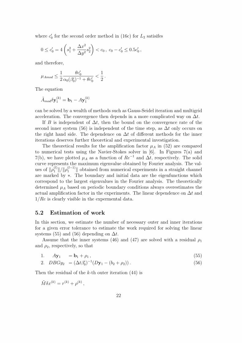
The theoretical results for the amplification factor µA in (52) are comparedto numerical tests using the Navier-Stokes solver in [6]. In Figures 7(a) and7(b), we have plotted µA as a function of Re−1 and ∆t, respectively. The solidcurve represents the maximum eigenvalue obtained by Fourier analysis. The val-ues of ‖ρ(l)

1 ‖/‖ρ(l−1)1 ‖ obtained from numerical experiments in a straight channel

are marked by ∗. The boundary and initial data are the eigenfunctions whichcorrespond to the largest eigenvalues in the Fourier analysis. The theoreticallydetermined µA based on periodic boundary conditions always overestimates theactual amplification factor in the experiments. The linear dependence on ∆t and1/Re is clearly visible in the expermental data.

5.2 Estimation of work

In this section, we estimate the number of necessary outer and inner iterationsfor a given error tolerance to estimate the work required for solving the linearsystems (55) and (56) depending on ∆t.

Assume that the inner systems (46) and (47) are solved with a residual ρ1

and ρ2, respectively, so that

1. Ay1 = b1 + ρ1 , (55)

2. DBGy2 = (∆tβi0)−1(Dy1 − (b2 + ρ2)) . (56)

Then the residual of the k-th outer iteration (44) is

Mδx(k) = r(k) + ρ(k) ,

22

2 3 4 5 6 7 8 9 10

x 10−3

0

0.002

0.004

0.006

0.008

0.01

0.012

0.014

0.016

0.018

0.02

1/Re

µ A

(a) ∆t = 0.05

0.01 0.015 0.02 0.025 0.03 0.035 0.04 0.045 0.050

1

2

3

4

5

6

7x 10

−3

∆ t

µ A

(b) Re = 300

Figure 7: Amplification factor µA in (52). The theoretical estimate of µA (solidline) is compared to experimental values (∗).

with ρ(k) = (ρT1 , ρT

2 )T . If we assume, that ‖ρ(j)‖ ≤ εi and ‖I −MM−1‖ ≤ µM ,then it is shown in [6] that

‖r(k)‖ ≤ µkM‖r(0)‖+ (1 + µM)

1− µkM

1− µM

εi .

A sufficient condition for convergence of the outer iteration in this norm is µM <1.

The convergence requirement on the residual of the outer iteration (44) is

‖r(k)‖ ≤ εo .

Then the maximum number of iterations is

k = dlog

((1− µM)εo − εi

(1− µM)‖r(0)‖ − εo

)/ log µMe ,

where dae denotes the smallest integer aI such that aI ≥ a. For our furtherconsiderations, we assume that an even distribution of the error coming from theinner iterations and the outer iteration is favorable. Then

µkM‖r(0)‖ =

εo

2and

1− µkM

1− µM

εi =εo

2, (57)

and consequently

k = dlog

(εo

2‖r(0)‖)

/log µMe . (58)

23

For the error of the inner iterations, the assumption is that the error between thetwo systems to be solved is split evenly. With the fixed point iteration (48) tosolve (55), the number of iterations l is

εi/2 = µAl‖ρ(0)

1 ‖ .

From (57) we obtain

εi = (1− µM)‖r(0)‖ εo

2

‖r(0)‖ − εo

2

,

and the number of necessary inner iterations can be calculated to be

l = dlog

(εi

2‖ρ(0)1 ‖

)/log µAe = dlog

((1− µM)

‖r(0)‖ εo

2

‖r(0)‖ − εo

2

1

2‖ρ(0)1 ‖

)/log µAe.

(59)

The total work necessary to solve the Navier Stokes equations over a fixedtime interval mainly consists of two parts: the solution of (55) and (56) in everyouter iteration in every time step. Denote by WA the work associated with the Asystem (55) and by WDBG the work associated with (56). For each time step, k Asystems have to be solved. The solution is computed with a fixed point iterationusing l steps and

WA ∼ 1

∆tkl.

Similarly, for each time step, k discrete Poisson-like systems need to be solved.In [6] the equations are solved with BiCGSTAB [36]. Other alternatives arethe generalized minimum residual method (GMRES) or the conjugate gradientmethod if DBG is symmetric and positive definite. While the convergence ratein the worst case is independent of ∆t if B is independent of ∆t, the initial guessx(0) in (44) may be more accurate for small ∆t if it is extrapolated from theprevious time step, thus reducing the work. For WDBG, we have

WDBG ∼ 1

∆tk.

In a periodic case, by Proposition 2 and (53) we have that µA ≈ 12θ/(α0(βi0)−1),

µM ≈ 12θ/(α0(βi0)−1 + 12θ) ≈ µA/(1 + µA) and θ ∼ ∆t. Thus, WA ∼ kl/µA

and WDBG ∼ k/µA. For a growing ∆t, k grows slowly, see (58) and Proposition2, and l grows quickly as ∆t approaches the the largest admissible time step∆t∗ = α0Re∆x2/12 from (53).

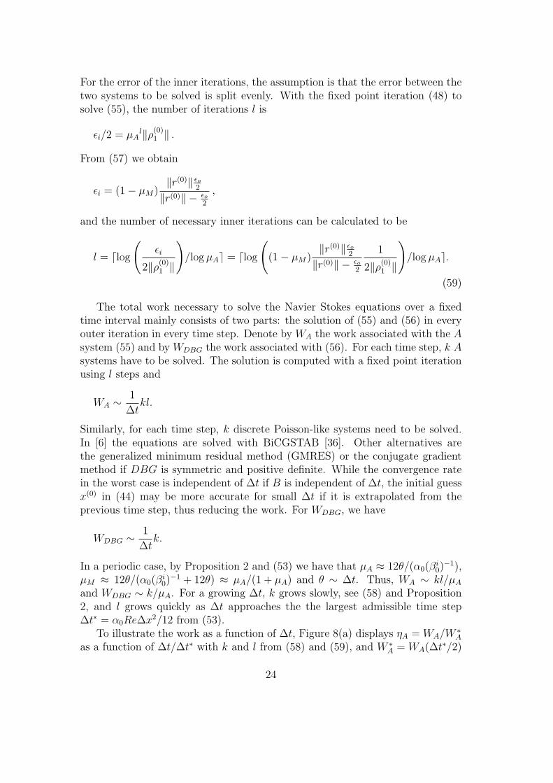
To illustrate the work as a function of ∆t, Figure 8(a) displays ηA = WA/W ∗A

as a function of ∆t/∆t∗ with k and l from (58) and (59), and W ∗A = WA(∆t∗/2)

24

0 0.2 0.4 0.6 0.8 10

2

4

6

8

10

12

∆ t / ∆ t*

η A

(a) ηA

0 0.2 0.4 0.6 0.8 10

2

4

6

8

10

12

14

16

∆ t / ∆ t*

η DB

G

(b) ηDBG

0 0.1 0.2 0.3 0.4 0.5 0.6 0.7 0.8 0.9 10

5

10

15

∆ t / ∆ t*

(10*

η DB

G+

η A)/

11

(c) 10ηDBG + ηA

Figure 8: Total relative work for the iterations as a function of ∆t/∆t∗.

25

0 0.5 1 1.5 2 2.5 3 3.5 4 4.5 50

0.5

1

1.5

2

2.5

3

3.5

θ

ξ

Euler

BDF2

Adams2

BDF3

BDF4

Adams3

Adams4

2nd order

4th order

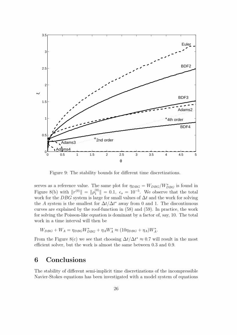
Figure 9: The stability bounds for different time discretizations.

serves as a reference value. The same plot for ηDBG = WDBG/W ∗DBG is found in

Figure 8(b) with ‖r(0)‖ = ‖ρ(0)1 ‖ = 0.1, εo = 10−5. We observe that the total

work for the DBG system is large for small values of ∆t and the work for solvingthe A system is the smallest for ∆t/∆t∗ away from 0 and 1. The discontinuouscurves are explained by the roof-function in (58) and (59). In practice, the workfor solving the Poisson-like equation is dominant by a factor of, say, 10. The totalwork in a time interval will then be

WDBG + WA = ηDBGW ∗DBG + ηAW ∗

A ≈ (10ηDBG + ηA)W ∗A.

From the Figure 8(c) we see that choosing ∆t/∆t∗ ≈ 0.7 will result in the mostefficient solver, but the work is almost the same between 0.3 and 0.9.

6 Conclusions

The stability of different semi-implicit time discretizations of the incompressibleNavier-Stokes equations has been investigated with a model system of equations

26

in Fourier space. The size of the stability domain for the CFL-numbers uλx andvλy depends on the parameter θ = ∆t/(Re∆x2). The time step limits with thelinear theory overestimate the limits obtained experimentally with a solver of theNavier-Stokes equations, but the trend is correctly predicted.

The time and length scales for wall bounded turbulent flow are derived. Anumber of points per unit length is chosen depending on the order of the methodyielding ∆t and ∆x. The requirements on uλx and θ for sufficient accuracy inthe boundary layer depend only on the number of points needed to resolve thescales in time and space.

One system of linear equations is solved iteratively in each time step for thevelocity and the pressure in an outer iteration and two or three inner iterations.Conditions for the outer iteration to converge for ∆t > 0 are given. The equa-tions to be solved in every outer iterative step are similar for many strategiesto solve the Navier-Stokes equations. A particular choice of inner iterations isanalyzed and one part of them imposes conditions on ∆t for convergence. Thetotal work for integration in a time interval is estimated and it grows rapidly as∆t approaches the convergence limit.

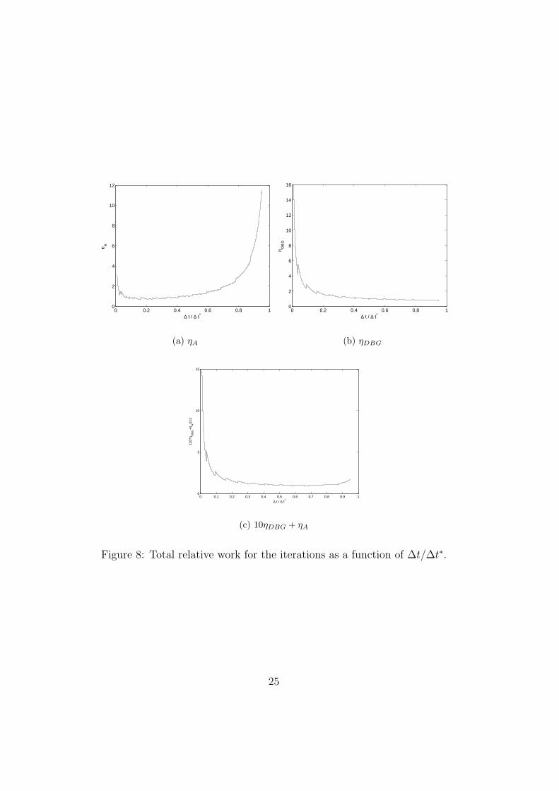
The stability domains for the semi-implicit methods of the BDF and Adamsfamilies up to fourth order are displayed in Figure 9. The bound on the CFL-number ξ = uλx with v = 0 is plotted as a function of θ. The BDF methodshave better stability properties than their Adams counterpart of the same order.The requirements for sufficient accuracy on ξ and θ in a turbulent boundary layerare marked by ∗ for the discretizations of fourth order in space (nl = 4 in (36))and second (nt = 10) and fourth (nt = 4) order in time. The second order markis well within the stability domain for BDF2. Accuracy decides which ξ and θto choose and ∆t is given by ξ, θ, and (36). The ξ and θ for sufficient accuracyin the fourth order case are not stable with BDF4. By decreasing ∆t so that ξand θ move along the dotted line, they are inside the stability domain at aboutθ = 2.5 and the scheme is then both accurate and stable. Stability determinesthe largest possible time step in this case. Note that it is possible to decrease ∆tin this way and obtain stability for all the methods in the figure, no matter whatthe accuracy requirements are on ξ and θ. If the fixed point iteration in (52) isapplied to solve the momentum equation, then θ and ∆t are constrained by (53)and further reduction along the dotted line is necessary.

With an inner iteration with a more favorable behavior for growing time stepsthan in Figure 8(a), Figure 8(b) indicates what we can expect: the total workdecreases with longer time steps. Then the bound on ∆t is imposed by accuracyor stability. From Figure 9 we conclude that BDF4 allows larger θ (and ∆t) thanBDF2 and therefore appears to be the most efficient alternative for wall boundedturbulent flow. The only disadvantage with BDF4 is that two more solutionvectors must be stored.

27

Acknowledgment

Valuable input to the discussion in Sect. 4 was provided by Arne Johansson andArnim Bruger pointed out the references [1, 29] to us. This work was supportedby the Swedish Foundation for Strategic Research.

References

[1] K. Alvelius, Studies of turbulence and its modelling through large eddy-and direct numerical simulation, PhD thesis, Dept of Mechanics, Royal In-stitute of Technology, Stockholm, Sweden, 1999.

[2] S. Armfield, R. Street, The fractional-step method for the Navier-Stokes equations on staggered grids: The accuracy of three variations, J.Comput. Phys., 153 (1999), 660–665.

[3] J. B. Bell, P. Colella, H. M. Glaz, A second- order projection methodfor the incompressible Navier Stokes eqautions, J. Comput. Phys., 85 (1989),257–283.

[4] K. Bhaganagar, D. Rempfer, J. Lumley, Direct numerical simulationof spatial transition to turbulence using fourth-order vertical velocity second-order vertical vorticity formulation, J. Comput. Phys., 180 (2002), 200–228.

[5] D. L. Brown, R. Cortez, M. L. Minion, Accurate projection meth-ods for the incompressible Navier-Stokes equations, J. Comput. Phys., 168(2001), 464–499.

[6] A. Bruger, B. Gustafsson, P. Lotstedt, J. Nilsson, High orderaccurate solution of the incompressible Navier-Stokes equations, Technicalreport 2003-064, Dept of Information Technology, Uppsala University, Upp-sala, Sweden, 2003, available at http://www.it.uu.se/research/reports/.

[7] A. Bruger, B. Gustafsson, P. Lotstedt, J. Nilsson, Splitting meth-ods for high order solution of the incompressible Navier-Stokes equations in3D, presented at ICFD Conference on Numerical Methods for Fluid Dynam-ics, Oxford, UK, March, 2004.

[8] A. Bruger, J. Nilsson, W. Kress, A compact higher order finite differ-ence method for the incompressible Navier-Stokes equations, J. Sci. Com-put., 17 (2002), 551–560.

[9] J. Cahouet, J.-P. Chabard, Some fast 3D finite element solvers for thegeneralized Stokes problem, Int. J. Numer. Meth. Fluids, 8 (1988), 869–895.

28

[10] W. Chang, F. Giraldo, B. Perot, Analysis of an exact fractional stepmethod, J. Comput. Phys., 180 (2002), 183–199.

[11] H. Choi, P. Moin, Effects of the computational time step on numericalsolutions of turbulent flow, J. Comput. Phys., 113 (1994), 1–4.

[12] A. J. Chorin, Numerical solution of the Navier-Stokes equations, Math.Comp., 22 (1968), 745–762.

[13] J. K. Dukowicz, A. S. Dvinsky, Approximate factorization as a highorder splitting for the implicit incompressible flow equations, J. Comput.Phys., 102 (1992), 336–347.

[14] W. E and J.-G. Liu, Projection method I: Convergence and numericalboundary layers, SIAM J. Numer. Anal., 32 (1995), 1017–1057.

[15] H. C. Elman, V. E. Howle, J. N. Shadid, R. S. Tuminaro, A paral-lel block multi-level preconditioner for the 3D incompressible Navier-Stokesequations, J. Comput. Phys., 187 (2003), 504–523.

[16] R. Friedrich, T. J. Huttl, M. Manhart, C. Wagner, Direct numer-ical simulation of incompressible turbulent flows, Computers & Fluids, 30(2001), 555–579.

[17] B. Gustafsson, P. Lotstedt, A. Goran, A fourth order differencemethod for the incompressible Navier-Stokes equations, in Numerical simu-lations of incompressible flows, ed. M.M. Hafez, World Scientific Publishing,Singapore, 2003, 263–276.

[18] E. Hairer, S. P. Nørsett, G. Wanner, Solving Ordinary DifferentialEquations I, Nonstiff Problems, 2nd ed., Springer-Verlag, Berlin, 1993.

[19] E. Hairer, G. Wanner, Solving Ordinary Differential Equations II, Stiffand Differential-Algebraic Problems, 2nd ed., Springer-Verlag, Berlin, 1996.

[20] G. E. Karniadakis, M. Israeli, S. A. Orszag, High-order splittingmethods for incompressible Navier-Stokes equations, J. Comput. Phys., 97(1991), 414–443.

[21] J. Kim, P. Moin, Application of a fractional-step method to incompressibleNavier-Stokes equations, J. Comput. Phys., 59 (1985), 308–323.

[22] W. Kress, J. Nilsson, Boundary conditions and estimates for the lin-earized Navier-Stokes equations on a staggered grid, Computers & Fluids,32 (2003), 1093–1112.

29

[23] S. K. Lele, Compact finite difference schemes with spectral-like resolution,J. Comput. Phys., 103 (1992), 16–42.

[24] R. Lohner, Multistage explicit advective prediction for projection-type in-compressible flow solvers, J. Comput. Phys., 195 (2004), 143–152.

[25] A. Lundbladh, D. S. Henningson, A. V. Johansson, An efficientspectral integration method for the solution of the time-dependent Navier-Stokes equations, Report FFA-TN 1992-28, Aeronautical Research Instituteof Sweden, Bromma, Sweden, 1992.

[26] M. L. Minion, On the stability of Godunov-projection methods for incom-pressible flow, J. Comput. Phys., 123 (1996), 435–449.

[27] S. Nagarajan, S. K. Lele, J. H. Ferziger, A robust high-order com-pact method for large eddy simulation, J. Comput. Phys., 191 (2003), 392–419.

[28] J. Nilsson, B. Gustafsson, P. Lotstedt, A. Bruger, High orderdifference method on staggered, curvilinear grids for the incompressibleNavier-Stokes equations, in Proceedings of Second MIT Conference on Com-putational Fluid and Solid Mechanics 2003, ed. K.J. Bathe, Elsevier, 2003,1057–1061.

[29] J. M. Osterlund, Experimental studies of zero pressure-gradient turbu-lent boundary layer flow, PhD thesis, Dept of Mechanics, Royal Institute ofTechnology, Stockholm, Sweden, 1999.

[30] J. B. Perot, An analysis of the fractional step method, J. Comput. Phys.,108 (1993), 51–58.

[31] A. Quarteroni, F. Saleri, A. Veneziani, Factorization methods forthe numerical approximation of Navier-Stokes equations, Comput. MethodsAppl. Mech. Engrg., 118 (2000), 505–526.

[32] H. Schlichting, Boundary-Layer Theory, McGraw-Hill, New York, 2001.

[33] R. Temam, Sur l’approximation de la solution des equations de Navier-Stokes par la methode des pas fractionnaires, II, Arch. Rational Mech. Anal.,33 (1969), 377–385.

[34] S. Turek, A comparative study of time-stepping techniques for the incom-pressible Navier-Stokes equations: From fully implicit non-linear schemes tosemi-implicit projection methods, Int. J. Numer. Meth. Fluids, 37 (1999),37–47.

30

[35] A. Veneziani, Block factorized preconditioners for high-order accurate intime approximation of the Navier-Stokes equations, Numer. Meth. Part.Diff. Eq., 19 (2003), 487–510.

[36] H. A. van der Vorst, BiCGSTAB: A fast and smoothly converging vari-ant of Bi-CG for the solution of nonsymmetric linear systems, SIAM J. Sci.Comput., 13 (1992), 631–644.

[37] J. van Kan, A second-order accurate pressure correction scheme for viscousincompressible flow, SIAM J. Sci. Stat. Comp., 7 (1986), 870–891.

[38] D. C. Wilcox, Turbulence Modeling for CFD, DCW Industries, La Canada,CA, 1994.

31