Asymptotic analysis of the navier-stokes equations
34
Topological Methods in Nonlinear Analysis Journal of the Juliusz Schauder Center Volume 10, 1997, 249–282 ASYMPTOTIC ANALYSIS OF THE NAVIER–STOKES EQUATIONS IN THIN DOMAINS I. Moise — R. Temam — M. Ziane Dedicated to O. A. Ladyzhenskaya 0. Introduction We are interested in this article with the Navier–Stokes equations of viscous incompressible fluids in three dimensional thin domains. Let Ω ε be the thin domain Ω ε = ω × (0,ε), where ω is a suitable domain in R 2 and 0 <ε< 1. Our aim is to derive an asymptotic expansion of the strong solution u ε of the Navier–Stokes equations in the thin domain Ω ε when ε is small, which is valid uniformly in time. This study should give a better understanding of the global existence results in thin domains obtained previously; see [15]–[17] and [23], [22]. We consider in this work two types of boundary conditions: the Dirichlet-periodic boundary condition and the purely periodic condition. For the first type of boundary condition we derive an asymptotic expansion of the solution u ε in terms of the solution of the associated Stokes problem. More precisely, we prove that the solution can be written, for ε small, as u ε (t)= w ε + u ε exp - νt 2ε 2 , ∀t> 0, where w ε is the solution of the associated Stokes problem and u ε is a bounded (in time) function depending on the initial data. We also give a new proof and an improvement of the global existence result obtained in [23]. 1991 Mathematics Subject Classification. 34C35, 35Q30, 76D05. Key words and phrases. Navier–Stokes equations, global existence of strong solutions, asymptotic analysis. c 1997 Juliusz Schauder Center for Nonlinear Studies 249
-
Upload
independent -
Category
Documents
-
view
1 -
download
0
Transcript of Asymptotic analysis of the navier-stokes equations

Topological Methods in Nonlinear AnalysisJournal of the Juliusz Schauder CenterVolume 10, 1997, 249–282
ASYMPTOTIC ANALYSIS OF THENAVIER–STOKES EQUATIONS IN THIN DOMAINS
I. Moise — R. Temam — M. Ziane
Dedicated to O. A. Ladyzhenskaya
0. Introduction
We are interested in this article with the Navier–Stokes equations of viscousincompressible fluids in three dimensional thin domains. Let Ωε be the thindomain Ωε = ω × (0, ε), where ω is a suitable domain in R2 and 0 < ε < 1.
Our aim is to derive an asymptotic expansion of the strong solution uε ofthe Navier–Stokes equations in the thin domain Ωε when ε is small, which isvalid uniformly in time. This study should give a better understanding of theglobal existence results in thin domains obtained previously; see [15]–[17] and[23], [22]. We consider in this work two types of boundary conditions: theDirichlet-periodic boundary condition and the purely periodic condition. Forthe first type of boundary condition we derive an asymptotic expansion of thesolution uε in terms of the solution of the associated Stokes problem. Moreprecisely, we prove that the solution can be written, for ε small, as
uε(t) = wε + uε exp(− νt
2ε2
), ∀t > 0,
where wε is the solution of the associated Stokes problem and uε is a bounded(in time) function depending on the initial data. We also give a new proof andan improvement of the global existence result obtained in [23].
1991 Mathematics Subject Classification. 34C35, 35Q30, 76D05.
Key words and phrases. Navier–Stokes equations, global existence of strong solutions,asymptotic analysis.
c©1997 Juliusz Schauder Center for Nonlinear Studies
249
250 I. Moise — R. Temam — M. Ziane
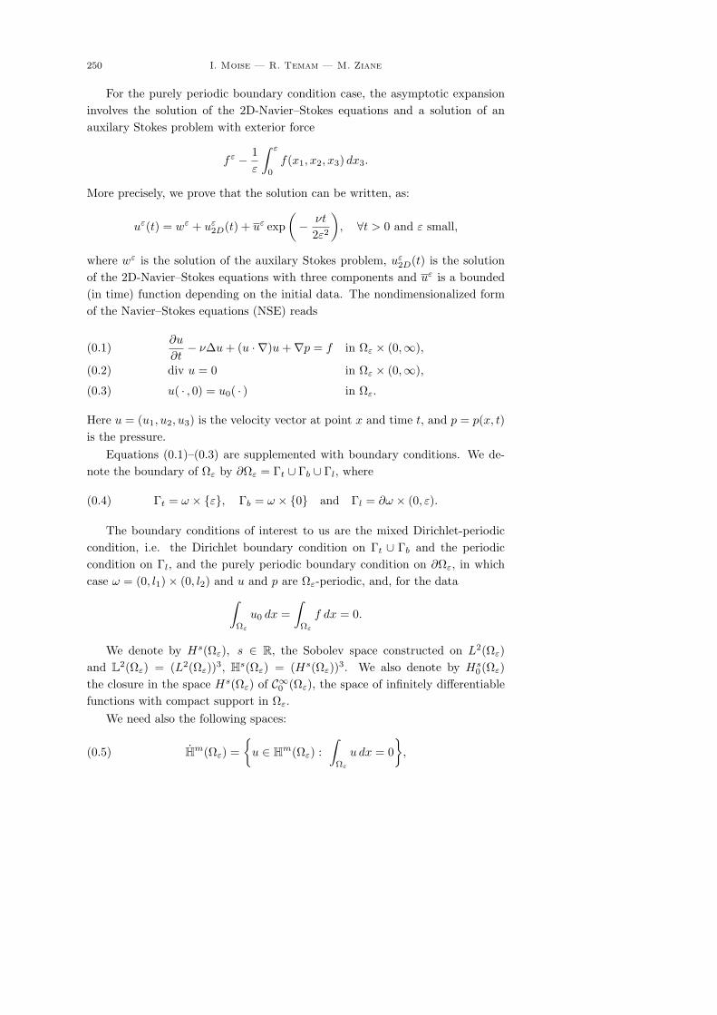
For the purely periodic boundary condition case, the asymptotic expansioninvolves the solution of the 2D-Navier–Stokes equations and a solution of anauxilary Stokes problem with exterior force
fε − 1ε
∫ ε
0
f(x1, x2, x3) dx3.
More precisely, we prove that the solution can be written, as:
uε(t) = wε + uε2D(t) + uε exp
(− νt
2ε2
), ∀t > 0 and ε small,
where wε is the solution of the auxilary Stokes problem, uε2D(t) is the solution
of the 2D-Navier–Stokes equations with three components and uε is a bounded(in time) function depending on the initial data. The nondimensionalized formof the Navier–Stokes equations (NSE) reads
∂u
∂t− ν∆u + (u · ∇)u +∇p = f in Ωε × (0,∞),(0.1)
div u = 0 in Ωε × (0,∞),(0.2)
u( · , 0) = u0( · ) in Ωε.(0.3)
Here u = (u1, u2, u3) is the velocity vector at point x and time t, and p = p(x, t)is the pressure.
Equations (0.1)–(0.3) are supplemented with boundary conditions. We de-note the boundary of Ωε by ∂Ωε = Γt ∪ Γb ∪ Γl, where
(0.4) Γt = ω × ε, Γb = ω × 0 and Γl = ∂ω × (0, ε).
The boundary conditions of interest to us are the mixed Dirichlet-periodiccondition, i.e. the Dirichlet boundary condition on Γt ∪ Γb and the periodiccondition on Γl, and the purely periodic boundary condition on ∂Ωε, in whichcase ω = (0, l1)× (0, l2) and u and p are Ωε-periodic, and, for the data∫
Ωε
u0 dx =∫
Ωε
f dx = 0.
We denote by Hs(Ωε), s ∈ R, the Sobolev space constructed on L2(Ωε)and L2(Ωε) = (L2(Ωε))3, Hs(Ωε) = (Hs(Ωε))3. We also denote by Hs
0(Ωε)the closure in the space Hs(Ωε) of C∞0 (Ωε), the space of infinitely differentiablefunctions with compact support in Ωε.
We need also the following spaces:
(0.5) Hm(Ωε) =
u ∈ Hm(Ωε) :∫
Ωε
u dx = 0
,

Asymptotic Analysis of NSE in Thin Domains 251
and the spaces Hmper(Ωε), which are defined with the help of Fourier series; we
write
(0.6) u(x) =∑k∈Z3
uk exp(
2ik · x
L
),
with uk = u−k (so that u is real valued) and
x
L=
(x1
l1,x2
l2,x3
ε
), k · x
L= k1
x1
l1+ k2
x2
l2+ k3
x3
ε.
Then, u is in L2(Ωε) if and only if
|u|2L2(Ωε) = εl1l2∑k∈Z3
|uk|2 < ∞,
and u is said to be in Hsper(Ωε), s ∈ R+, if and only if∑
k∈Z3
(1 + |k|2)s|uk|2 < ∞.
For the mathematical setting of the Navier–Stokes equations, we classicallyconsider a Hilbert space Hε, which is a closed subspace of L2(Ωε). Dependingon the boundary condition, we define the following:
HP = HεP =
u ∈ L2(Ωε) : div u = 0,
∫Ωε
u dx = 0,
uj is periodic in the direction xj , j = 1, 2, 3
in the case of the purely periodic boundary condition, and
HDP = HεDP =
u ∈ L2(Ωε) : div u = 0, u3 = 0 on Γt ∪ Γb,
∫Ωε
uα dx = 0,
and uα is periodic in the direction xα, α = 1, 2
,
in the case of the mixed Dirichlet-periodic boundary condition.Another useful space is Vε, a closed subspace of H1(Ωε), which is defined as
follows depending on the boundary condition:
VP = V εP =
u ∈ H1
per(Ωε) : div u = 0,
VDP = V εDP =
u ∈ H1(Ωε) ∩HDP : u = 0 on Γt ∪ Γb
and u is periodic in the directions x1 and x2
,
The scalar product on Hε is denoted by ( · , · )ε, the one on Vε is denoted by(( · , · ))ε, and the associated norms are denoted by | · |ε and || · ||ε respectively.We denote by Aε the Stokes operator defined as an isomorphism from Vε ontothe dual V ′ε of Vε, by
(0.7) 〈Aεu, v〉V ′ε ,Vε
= ((u, v))ε, ∀v ∈ Vε.

252 I. Moise — R. Temam — M. Ziane
The operator Aε is extended to Hε as a linear unbounded operator. The domainof Aε in Hε is denoted by D(Aε). The space D(Aε) can be fully characterizedusing the regularity theory. We refer for the study of the regularity of the Stokesoperator to [2], [6], [10], [12], [18]–[20] and [24].
Let bε be the continuous trilinear form on Vε defined by
(0.8) bε(u, v, w) =3∑
i,j=1
∫Ωε
ui∂vj
∂xiwj dx, u, v, w ∈ Vε.
We denote by Bε the bilinear form on Vε defined for (u, v) ∈ Vε × Vε by
〈Bε(u, v), w〉V ′ε ,Vε
= bε(u, v, w), ∀w ∈ Vε,
and we set Bε(u) = Bε(u, u).We assume in this article that the data ν, u0 and f satisfy
(0.9) ν > 0, u0 ∈ Hε (or Vε), f ∈ L∞(0,∞;Hε).
The system of equations (0.1)–(0.3), with one of the boundary conditionslisted above, can be written as a differential equation in V ′ε
(0.10)
u′ + νAεu + Bε(u) = f,
u(0) = u0,
where u′ denotes the derivative (in the distribution sense) of the function u withrespect to time. We recall now the classical result of existence of solutions toproblem (0.10). See e.g. [4], [9], [10], [14], [19], [20].
Theorem 0.1. For u0 ∈ Hε, there exists a solution (not necessarily unique)u = uε to problem (0.10) such that
(0.11) uε ∈ L2(0, T ;Vε) ∩ L∞(0, T ;Hε), ∀T > 0.
Moreover, if u0 ∈ Vε, then there exists Tε = Tε(Ωε, ν, u0, f) > 0 and a uniquesolution uε to problem (0.10) such that
(0.12) uε ∈ L2(0, Tε;D(Aε)) ∩ L∞(0, Tε;Vε).
The solution uε which satisfies (0.12) is called the strong solution of (0.10).
1. Functional inequalities in thin domains
In this section we present some functional inequalities in thin domains. Wewill only state the inequalities without proofs and we refer the reader to [23] fora detailed discussion. The functional inequalities considered here are Sobolev-type inequalities and the Cattabriga–Solonnikov regularity inequality for theStokes operator. We should mention that in the classical Sobolev inequalities,the constants are dilation invariant but do, however, depend on the shape of
Asymptotic Analysis of NSE in Thin Domains 253
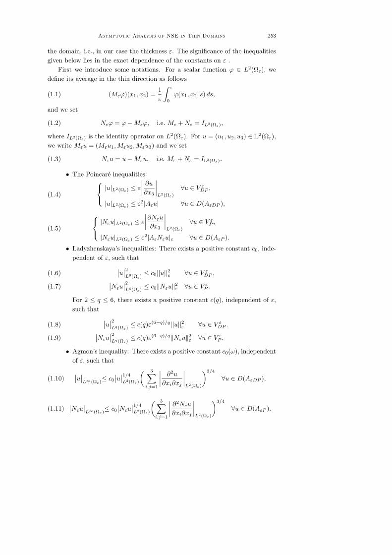
the domain, i.e., in our case the thickness ε. The significance of the inequalitiesgiven below lies in the exact dependence of the constants on ε .
First we introduce some notations. For a scalar function ϕ ∈ L2(Ωε), wedefine its average in the thin direction as follows
(1.1) (Mεϕ)(x1, x2) =1ε
∫ ε
0
ϕ(x1, x2, s) ds,
and we set
(1.2) Nεϕ = ϕ−Mεϕ, i.e. Mε + Nε = IL2(Ωε),
where IL2(Ωε) is the identity operator on L2(Ωε). For u = (u1, u2, u3) ∈ L2(Ωε),we write Mεu = (Mεu1,Mεu2,Mεu3) and we set
(1.3) Nεu = u−Mεu, i.e. Mε + Nε = IL2(Ωε).
• The Poincare inequalities:
(1.4)
|u|L2(Ωε) ≤ ε
∣∣∣∣ ∂u
∂x3
∣∣∣∣L2(Ωε)
∀u ∈ V εDP ,
|u|L2(Ωε) ≤ ε2|Aεu| ∀u ∈ D(AεDP ),
(1.5)
|Nεu|L2(Ωε) ≤ ε
∣∣∣∣∂Nεu
∂x3
∣∣∣∣L2(Ωε)
∀u ∈ V εP ,
|Nεu|L2(Ωε) ≤ ε2|AεNεu|ε ∀u ∈ D(AεP ).
• Ladyzhenskaya’s inequalities: There exists a positive constant c0, inde-pendent of ε, such that∣∣u∣∣2
L6(Ωε)≤ c0||u||2ε ∀u ∈ V ε
DP ,(1.6) ∣∣Nεu∣∣2L6(Ωε)
≤ c0‖Nεu‖2ε ∀u ∈ V ε
P .(1.7)
For 2 ≤ q ≤ 6, there exists a positive constant c(q), independent of ε,such that ∣∣u∣∣2
Lq(Ωε)≤ c(q)ε(6−q)/q||u||2ε ∀u ∈ V ε
DP .(1.8) ∣∣Nεu∣∣2Lq(Ωε)
≤ c(q)ε(6−q)/q‖Nεu‖2ε ∀u ∈ V ε
P .(1.9)
• Agmon’s inequality: There exists a positive constant c0(ω), independentof ε, such that
(1.10)∣∣u∣∣
L∞(Ωε)≤ c0
∣∣u∣∣1/4
L2(Ωε)
( 3∑i,j=1
∣∣∣∣ ∂2u
∂xi∂xj
∣∣∣∣L2(Ωε)
)3/4
∀u ∈ D(AεDP ),
(1.11)∣∣Nεu
∣∣L∞(Ωε)
≤ c0
∣∣Nεu∣∣1/4
L2(Ωε)
( 3∑i,j=1
∣∣∣∣ ∂2Nεu
∂xi∂xj
∣∣∣∣L2(Ωε)
)3/4
∀u ∈ D(AεP ).

254 I. Moise — R. Temam — M. Ziane
• Cattabriga–Solonnikov inequality: There exists a positive constantc0(ω), independent of ε, such that
3∑i,j=1
∣∣∣∣ ∂2u
∂xi∂xj
∣∣∣∣2L2(Ωε)
≤ c0
∣∣Aεu∣∣2L2(Ωε)
, ∀u ∈ D(Aε).
2. The Dirichlet-periodic boundary condition
In this section we derive an asymptotic expansion of the solution uε of theNavier–Stokes equations in the thin domains Ωε, when ε goes to zero. Theboundary condition under consideration is the mixed Dirichlet-periodic condi-tion. It is shown in [23] that the H1-norm of uε converges to zero when ε goes tozero. Hence, one expects, in this case, a slow motion of the fluid. Our purpose inthis section is to establish rigourously that the fluid has slow motion and to findthe leading term. For this purpose, we first compare the solution of the nonlinearstationary problem to the solution of the Stokes problem (the linear problem).Then, we compare the solution of the evolutionary problem to the solution ofthe nonlinear stationary problem. This yields an asymptotic expression of thesolution uε when ε is small.
2.1. Comparison between the nonlinear stationary problem andthe Stokes problem. Consider the steady state Navier–Stokes equations inthe thin domain Ωε
− ν∆vε + (vε · ∇)vε +∇qε = fε in Ωε,(2.1)
div vε = 0 in Ωε,(2.2)
vε = 0 on ω × 0, ε,(2.3)
vε is periodic in the directions x1 and x2.(2.4)
First, note using (1.4), that
(2.5) ν∣∣A1/2
ε vε∣∣2ε
= (fε, vε) ≤ |fε|ε|vε|ε ≤ ε|fε|ε∣∣A1/2
ε vε∣∣ε.
Hence
(2.6)∣∣A1/2
ε vε∣∣2ε≤ ε2|fε|2ε/ν2.
Let wε be the unique solution of the Stokes problem:
− ν∆wε +∇qε = fε in Ωε,(2.7)
div wε = 0 in Ωε,(2.8)
wε = 0 on ω × 0, ε,(2.9)
wε is periodic in the directions x1 and x2.(2.10)

Asymptotic Analysis of NSE in Thin Domains 255
We note that
(2.11)∣∣A1/2
ε wε∣∣2ε≤ ε2|fε|2ε/ν2.
Now we write the equations satisfied by V ε = vε − wε and Qε = qε − qε. Wehave
(2.12)
−ν∆V ε + (V ε · ∇)V ε +∇Qε
= −(wε · ∇)V ε − (V ε · ∇)wε − (wε · ∇)wε in Ωε,
div V ε = 0 in Ωε,
and the boundary condition
(2.13)
V ε = 0 on ω × 0, ε,V ε is periodic in the directions x1 and x2.
We multiply (2.12) with V ε, integrate over Ωε and obtain
(2.14) ν∣∣A1/2
ε V ε∣∣2ε
= −∫
Ωε
(V ε · ∇)wε · V ε dx−∫
Ωε
(wε · ∇)wε · V ε dx,
and with ∣∣∣∣ ∫Ωε
(V ε · ∇)wε · V ε dx
∣∣∣∣ ≤ |V ε|2L4(Ωε)|A1/2ε wε|ε(2.15)
≤ c0ε1/2|A1/2
ε V ε|2ε|A1/2ε wε|ε
and ∣∣∣∣∫Ωε
(wε · ∇)wε · V εdx
∣∣∣∣ ≤ ∣∣wε∣∣L4(Ωε)
∣∣A1/2ε wε
∣∣ε
∣∣V ε∣∣L4(Ωε)
(2.16)
≤ c0ε1/2
∣∣A1/2ε wε
∣∣2ε
∣∣A1/2ε V ε
∣∣ε,
we have
ν∣∣A1/2
ε V ε∣∣2ε≤ c0ε
1/2∣∣A1/2
ε V ε∣∣2ε
∣∣A1/2ε wε
∣∣ε
(2.17)
+ c0ε1/2
∣∣A1/2ε wε
∣∣2ε
∣∣A1/2ε V ε
∣∣ε
≤ c0ε1/2
∣∣A1/2ε V ε
∣∣2ε
∣∣A1/2ε wε
∣∣ε+ ν
∣∣A1/2ε V ε
∣∣2ε/2
+ c20 ε
∣∣A1/2ε wε
∣∣4ε/2ν.
Let R0 be a positive function defined on R+ and satisfying
(2.18) limε→0
εR20(ε) = 0
and choose ε1 such that, for 0 < ε ≤ ε1
(2.19) c0ε1/2R0(ε) ≤ ν/16.
Assume also (see (2.36)) that
(2.20) ε2|fε|2ε ≤ R20(ε)/ν2.

256 I. Moise — R. Temam — M. Ziane
We then infer from (2.11) and (2.17) that
(2.21)∣∣A1/2
ε V ε∣∣2ε≤ 2c2
0εR20(ε)
∣∣A1/2ε wε
∣∣2ε/ν2.
Thanks to (2.18) and (2.21),∣∣A1/2
ε V ε∣∣2ε
is negligeable compared to∣∣A1/2
ε wε∣∣2ε
forε small. We have proved the
Lemma 2.1. Let wε (resp. vε) be the solution of the Stokes problem (resp.the nonlinear stationary Navier–Stokes equations) in the thin domain Ωε. As-sume that (2.18)–(2.20) hold. Then we can write vε = wε + V ε, with V ε smallcompared to wε, i.e.,
(2.22) limε→0
∣∣A1/2ε V ε
∣∣2ε∣∣A1/2
ε wε∣∣2ε
= 0.
2.2. Comparison between the evolutionary and the stationary prob-lems. In this subsection we prove the global existence of the strong solutionuε(t) for ε small and show that up to a time boundary layer near t = 0, thesolution converges exponentially (in time) to a stationary solution of the Navier-Stokes equations. We also show that the convergence, when ε goes to zero, isexponential as long as the initial data belongs to a ball in H1 with radius lessthan ν/(16c0ε
1/2) and center vε, a solution of the stationary problem.Let Uε(t) = uε(t)− vε. The equations satisfied by Uε(t) are:
(2.23)
∂Uε
∂t− ν∆Uε + (Uε · ∇)Uε + (Uε · ∇)vε
+ (vε · ∇)Uε +∇(pε − qε) = 0 in Ωε,
div Uε = 0 in Ωε,
Uε = 0 on ω × 0, ε,Uε is periodic in the directions x1 and x2,
and the initial condition reads
(2.24) Uε(0) = uε0 − vε.
Using equations (2.23), we obtain
(2.25)12
d
dt
∣∣A1/2ε Uε(t)
∣∣2ε
+ ν∣∣AεU
ε(t)∣∣2ε
≤∣∣b(Uε, Uε, AεU
ε)∣∣ +
∣∣b(Uε, vε, AεUε)
∣∣ +∣∣b(vε, Uε, AεU
ε)∣∣,
and with inequalities (1.4), (1.8) and (1.10), we can write
(2.26)12
d
dt
∣∣A1/2ε Uε(t)
∣∣2ε
+ν
2
∣∣AεUε(t)
∣∣2ε
≤ c0ε1/2
∣∣A1/2ε Uε(t)
∣∣ε
∣∣AεUε(t)
∣∣2ε
+ c0ε1/2
∣∣A1/2ε vε
∣∣ε
∣∣AεUε(t)
∣∣2ε.

Asymptotic Analysis of NSE in Thin Domains 257
Hence,
(2.27)d
dt
∣∣A1/2ε Uε(t)
∣∣2ε
+[ν − 2c0ε
1/2∣∣A1/2
ε Uε(t)∣∣ε
− 2c0ε1/2
∣∣A1/2ε vε
∣∣ε
]∣∣AεUε(t)
∣∣2ε≤ 0.
With R0 defined as in (2.18), (2.19), we supplement (2.20) by assuming that
(2.28)∣∣A1/2
ε Uε0
∣∣2ε
+ ε2|fε|2ε/ν2 ≤ R20(ε).
Then there exists T (ε) > 0 such that
(2.29)∣∣A1/2
ε Uε(t)∣∣2ε≤ 4R2
0(ε) for 0 ≤ t ≤ T (ε).
Let [0, T (ε))
denote the maximal interval on which (2.29) holds. Note that ifT (ε) < ∞, then
(2.30)∣∣A1/2
ε Uε(T (ε))∣∣2ε
= 4 R20(ε).
We infer from (2.6) and (2.29) that
(2.31)d
dt
∣∣A1/2ε Uε(t)
∣∣2ε
+[ν − 16c0ε
1/2R0(ε)]∣∣AεU
ε(t)∣∣2ε≤ 0, 0 ≤ t ≤ T (ε).
Using (2.19) we see that for 0 < ε ≤ ε1 and 0 ≤ t ≤ T (ε), we have by thePoincare inequality
(2.32)d
dt
∣∣A1/2ε Uε(t)
∣∣2ε
+ν
2ε2
∣∣A1/2ε Uε(t)
∣∣2ε≤ 0,
which implies that∣∣A1/2
ε Uε(t)∣∣2ε
is decreasing as a function of t and thereforeT (ε) = +∞, for ε ≤ ε1. Moreover, we have∣∣A1/2
ε Uε(t)∣∣2ε≤
∣∣A1/2ε Uε
0
∣∣2εexp
(− νt
2ε2
)(2.33)
≤∣∣A1/2
ε uε0 −A1/2
ε vε∣∣2εexp
(− νt
2ε2
).
Finally, we write
(2.34) uε(t) = vε + Uε(t) = wε + V ε + Uε(t),
where wε is the unique solution of the Stokes problem with exterior force fε,and V ε and Uε(t) satisfy
(2.35)∣∣∣∣V ε
∣∣∣∣2ε≤ 2c2
0ε∣∣∣∣wε
∣∣∣∣4ε/ν2
and ∣∣∣∣Uε(t)∣∣∣∣2
ε≤
∣∣∣∣uε0 − wε − V ε
∣∣∣∣2εexp
(− νt
2ε2
), t ≥ 0

258 I. Moise — R. Temam — M. Ziane
Theorem 2.2. Let R0(ε) be a monotone positive function satisfying condi-tion limε→0 εR2
0(ε) = 0. Assume that vε is a solution of the stationary Navier–Stokes equations with exterior force fε in the domain Ωε, and
(2.36)∣∣∣∣uε
0 − vε∣∣∣∣2
ε+ ε2
∣∣fε∣∣2ε/ν2 ≤ R2
0(ε).
Then there exists ε1 = ε1(ν) such that for 0 < ε ≤ ε1, the maximal time T (ε)of existence of the strong solution uε(t) of the 3D-Navier–Stokes equations in Ωε
satisfies T (ε) = ∞, and for all t ≥ 0
(2.37)∣∣∣∣uε(t)− vε
∣∣∣∣2ε≤
∣∣∣∣uε0 − vε
∣∣∣∣2εexp
(− νt
2ε2
).
Moreover, if wε is the unique solution of the Stokes problem with exterior force fε,then
(2.38) uε(t) = wε + V ε + Uε(t), ∀t ≥ 0,
with
(2.39)∣∣∣∣V ε
∣∣∣∣2ε≤ c2
0
2νε R2
0(ε)∣∣∣∣wε
∣∣∣∣2ε
and for all t ≥ 0 ∣∣∣∣Uε(t)∣∣∣∣2
ε≤
∣∣∣∣uε0 − vε
∣∣∣∣2εexp
(− νt
2ε2
).
Remark 2.1. (i) We obtained in Theorem 2.1 an improvement for the globalregularity result obtained in [23]. Note that the conditions on the data are givenin (2.36); in particular, due to (2.19) uε
0 can belong to a ball in H1(Ωε) of centervε and radius ν/(16c0ε
1/2).(ii) We also obtained an asymptotic expansion for the solution uε(t) for ε
small which is uniformly valid in time. This asymptotic expansion suggests thatthe attractor of the dynamical system associated with the Navier–Stokes equa-tion with Dirichlet-periodic boundary condition in the thin domain Ωε reducesto the set of stationary solutions, when ε is small enough.
(iii) The solution wε to the stationary problem (2.7)–(2.10) which approx-imates vε and hence uε, can be itself approximated by a simpler expression,possibly an explicit one. For example, in the case of a pressure driven flow,
(2.40) fε = Pe1,
where P is constant (the pressure gradient), then wε ≈ ϕεe1, with
(2.41) ϕε = Px3(ε− x3)/2ν.
Note that since 0 < x3 < ε, ϕε is of order of ε2.
Asymptotic Analysis of NSE in Thin Domains 259
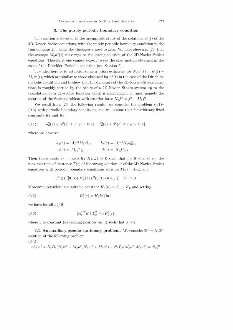
3. The purely periodic boundary condition
This section is devoted to the asymptotic study of the solutions uε(t) of the3D-Navier–Stokes equations, with the purely periodic boundary condition in thethin domains Ωε, when the thickness ε goes to zero. We have shown in [23] thatthe average Mεu
ε(t) converges to the strong solution of the 2D-Navier–Stokesequations. Therefore, one cannot expect to see the slow motion obtained in thecase of the Dirichlet–Periodic condition (see Section 2).
The idea here is to establish some a priori estimates for Nεuε(t) = uε(t) −
Mεuε(t), which are similar to those obtained for uε(t) in the case of the Dirichlet-
periodic condition, and to show that the dynamics of the 3D-Navier–Stokes equa-tions is roughly carried by the orbits of a 2D-Navier–Stokes system up to thetranslation by a 3D-vector function which is independent of time, namely thesolution of the Stokes problem with exterior force Nεf
ε = fε −Mεfε.
We recall from [23] the following result: we consider the problem (0.1)–(0.3) with periodic boundary conditions, and we assume that for arbitrary fixedconstants K1 and K2,
(3.1) a20(ε) + α2(ε) ≤ K1ε ln | ln ε|, b2
0(ε) + β2(ε) ≤ K2 ln | ln ε|,
where we have set
a0(ε) = |A1/2ε Mεu
ε0|ε, b0(ε) = |A1/2
ε Nεuε0|ε,
α(ε) = |Mεfε|ε, β(ε) = |Nεf
ε|ε.
Then there exists ε0 = ε0(ν,K1,K2, ω) > 0 such that for 0 < ε < ε0, themaximal time of existence T (ε) of the strong solution uε of the 3D-Navier–Stokesequations with periodic boundary conditions satisfies T (ε) = +∞, and
uε ∈ C([0,∞);V εP ) ∩ L2(0, T ;D(AεP )) ∀T > 0.
Moreover, considering a suitable constant K3(ν) > K1 + K2 and setting
(3.2) R20(ε) = K3 ln | ln ε|
we have for all t ≥ 0
(3.3) |A1/2ε uε(t)|2ε ≤ σR2
0(ε),
where σ is constant (depending possibly on ν) such that σ > 2.
3.1. An auxiliary pseudo-stationary problem. We consider w ε = Nεwε
solution of the following problem(3.4)νAεw
ε + NεBε(Nεwε + Mεu
ε, Nεwε + Mεu
ε)−NεBε(Mεuε,Mεu
ε) = Nεfε.

260 I. Moise — R. Temam — M. Ziane
Equivalently for all v ∈ Vp, w ε ∈ NεVP satisfies
(3.5) ν(A1/2ε Nεw
ε, A1/2ε Nεv)ε + bε(Nεw
ε, Nεwε, Nεv) + bε(Mεu
ε, Nεwε, Nεv)
+ bε(Nεwε,Mεu
ε, Nεv) = (Nεfε, Nεv)ε.
Since uε = uε(t), we shall consider the time as a parameter.The proof of the existence and uniqueness of w ε is standard (note that the
uniqueness holds if we consider ε small enough). We omit the details and willonly derive the estimates for ωε. For this purpose and throughout this section,we use extensively the following estimates on the trilinear form bε
Lemma 3.1. Let q ∈ (0, 1/2). There exists a positive constant c1(q), inde-pendent of ε, such that:
|bε(Mεu, Nεv, w)| ≤ c1εq|A1/2
ε Mεu|ε|AεNεv|ε|w|ε|bε(Nεv,Mεu, w)| ≤ c1ε
1/2|A1/2ε Mεu|ε|AεNεv|ε|w|ε
for all u ∈ D(A1/2ε ), v ∈ D(Aε), w ∈ L2(Ωε),
|bε(Nεu, Nεv, w)| ≤ c1|A1/2ε Nεu|1/2
ε |AεNεu|1/2ε |A1/2
ε Nεv|ε|w|ε≤ c1ε
1/2|AεNεu|ε|A1/2ε Nεv|ε|w|ε
for all u ∈ D(Aε), v ∈ D(A1/2ε ), w ∈ L2(Ωε),
|bε(Nεu, Nεv, w)| ≤ c1ε1/2|A1/2
ε Nεu|ε|AεNεv|ε|w|ε
for all u ∈ D(A1/2ε ), v ∈ D(Aε), w ∈ L2(Ωε).
This lemma is a slight generalization of Lemma 2.7 in [23]; we omit the detailsof the proof, which essentially relies on the functional inequalities (1.5), (1.7),(1.9) and (1.11).
Estimates for wε. We set Nεv = Nεwε in (3.5) and obtain
(3.6) ν|A1/2ε Nεw
ε|2ε + bε(Nεwε,Mεu
ε, Nεwε) = (Nεf
ε, Nεwε)ε,
which by (1.9) leads to
(3.7) ν|A1/2ε Nεw
ε|2ε≤ |Nεf
ε|ε|Nεwε|ε + c|Nεw
ε|2L4(Ωε)|A1/2ε Mεu
ε|ε
≤ ν
4|A1/2
ε Nεwε|2ε +
2ε2
ν|Nεf
ε|2ε + cε1/2|A1/2ε Nεw
ε|2ε|A1/2ε Mεu
ε|ε,
where c is a constant independent of ε.Now we take into account (3.2) and (3.3) and we obtain the existence of ε1
= ε1(ν, ω, K1,K2) such that for 0 < ε ≤ ε1,
(3.8) |A1/2ε Nεw
ε|2ε ≤ 4ε2|Nεfε|2e/ν2

Asymptotic Analysis of NSE in Thin Domains 261
We observe that | ddtNεw
ε|ε is small in a sense that we make precise now. Indeed,we differentiate (3.5) with respect to t and we obtain
ν
(d
dtA1/2
ε Nεwε, A1/2
ε Nεv
)ε
+ bε
(d
dtNεw
ε, Nεwε, Nεv
)(3.9)
+ bε
(Nεw
ε,d
dtNεw
ε, Nεv
)+ bε
(d
dtMεu
ε, Nεwε, Nεv
)+ bε
(Mεu
ε,d
dtNεw
ε, Nεv
)+ bε
(d
dtNεw
ε,Mεuε, Nεv
)+ bε
(Nεw
ε,d
dtMεu
ε, Nεv
)= 0.
For t > 0 fixed, we set v = A−1ε
ddtNεw
ε in (3.9) and we obtain
(3.10) ν
∣∣∣∣ d
dtNεw
ε
∣∣∣∣2ε
+ bε
(AεNεv,Nεw
ε, Nεv
)+ bε
(Nεw
ε, AεNεv,Nεv
)+ bε
(d
dtMεu
ε, Nεwε, Nεv
)+ bε
(Mεu
ε, AεNεv,Nεv
)+ bε
(AεNεv,Mεu
ε, Nεv
)+ bε
(Nεw
ε,d
dtMεu
ε, Nεv
)= 0,
so that, by Lemma 3.1, we obtain
ν
∣∣∣∣ d
dtNεw
ε
∣∣∣∣2ε
≤ 2c1ε1/2|A1/2
ε Nεwε|ε|AεNεv|2ε(3.11)
+ 2c1ε1/2
∣∣∣∣ d
dtMεu
ε
∣∣∣∣ε
|A1/2ε Nεw
ε|ε|AεNεv|ε
+ 2c1εq|A1/2
ε Mεuε|ε|AεNεv|2ε
Using (3.8), (3.2) and (3.3), we deduce that there exists ε2 = ε2(ν, ω,K1,K2)such that if 0 < ε ≤ ε2, then by (3.8)∣∣∣∣ d
dtNεw
ε
∣∣∣∣ε
≤ c
νε1/2
∣∣∣∣ d
dtMεu
ε
∣∣∣∣ε
|A1/2ε Nεw
ε|ε(3.12)
≤ c(ν)ε3/2
∣∣∣∣ d
dtMεu
ε
∣∣∣∣ε
|Nεfε|ε.
Now we need to bound∣∣ ddtMεu
ε∣∣ε
in terms of R20(ε). We have
(3.13)12
d
dt|A1/2
ε uε|2ε + ν|Aεuε|2ε + bε(uε, uε, Aεu
ε) = (fε, Aεuε)ε,
and therefore
(3.14)d
dt|A1/2
ε uε|2ε + ν|Aεuε|2ε ≤
c
ν|fε|2ε +
c
ν3|A1/2
ε uε|6ε,

262 I. Moise — R. Temam — M. Ziane
c being a numerical constant (independent of ε). Let t0 > 0 be an arbitrarlysmall time. We deduce from (3.1), (3.3) and (3.14) that
(3.15) ν
∫ t+t0
t
|Aεuε(s)|2ε ds ≤ c(ν)
[R2
0(ε) + R60(ε)
]t0, ∀t ≥ 0.
Since |duε/dt|ε ≤ ν|Aεuε|ε + |Bε(uε, uε)|ε + |fε|ε, a simple computation yields
(3.16)∫ t+t0
t
∣∣∣∣duε
dt
∣∣∣∣2ε
≤ c(ν)R20(ε)(1 + R2
0(ε))2t0, ∀t ≥ 0.
Now we differentiate (0.10) with respect to t and we obtain
(3.17)d2uε
dt2+ ν
d
dtAεu
ε + Bε
(duε
dt, uε
)+ Bε
(uε,
duε
dt
)= 0,
which leads then to
(3.18)12
d
dt
∣∣∣∣duε
dt
∣∣∣∣2ε
+ ν
∣∣∣∣A1/2ε
(duε
dt
)∣∣∣∣2ε
≤∣∣∣∣bε
(duε
dt, uε,
duε
dt
)∣∣∣∣≤ c
∣∣∣∣duε
dt
∣∣∣∣1/2
ε
∣∣∣∣A1/2ε
(duε
dt
)∣∣∣∣3/2
ε
|A1/2ε uε|ε,
c being a numerical constant (independent of ε). We infer from (3.18) that
(3.19)d
dt
∣∣∣∣duε
dt
∣∣∣∣2ε
≤ c
ν3|A1/2
ε uε|4ε∣∣∣∣duε
dt
∣∣∣∣2ε
.
We apply the uniform Gronwall lemma recalled below (see Lemma 3.2) with
y =∣∣∣∣duε
dt
∣∣∣∣2ε
, g =c
ν3|A1/2
ε uε|4ε, h = 0.
From (3.16) and (3.3), we infer the following estimates (say t0 ≤ 1)∫ t+t0
t
g(s) ds ≤ c(ν)R40(ε)t0 ≤ c(ν)R4
0(ε),∫ t+t0
t
y(s) ds ≤ c(ν)R20(ε)[1 + R2
0(ε)]2t0,
so that
(3.20)∣∣∣∣duε
dt
∣∣∣∣2ε
≤ c(ν)R20(ε)[1 + R2
0(ε)]2 exp(c(ν)R4
0(ε))
holds for every t ≥ t0 > 0. Since t0 > 0 is arbitrarily small and the right handside of (3.20) is independent of t0, (3.20) holds for (almost) every t > 0. We use(3.20) in (3.12) and we obtain
(3.21)∣∣∣∣ d
dtNεw
ε
∣∣∣∣ε
≤ c(ν)ε3/2R20(ε)[1 + R2
0(ε)] exp(c(ν)R40(ε)).
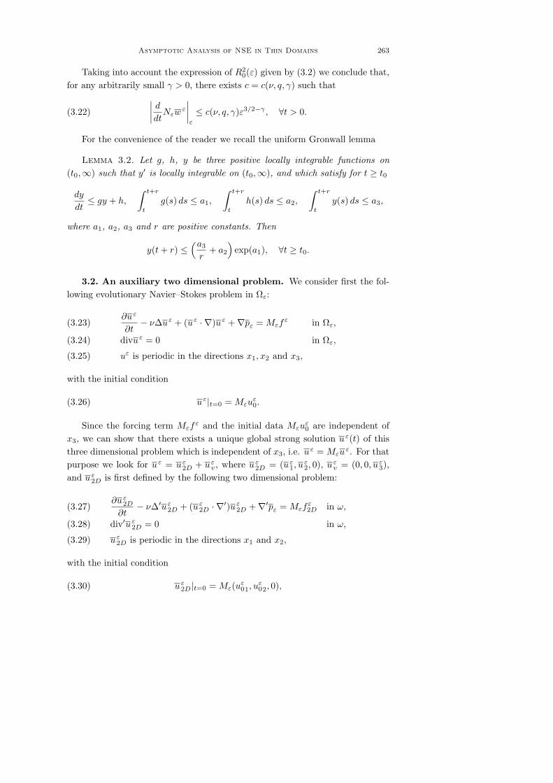
Asymptotic Analysis of NSE in Thin Domains 263
Taking into account the expression of R20(ε) given by (3.2) we conclude that,
for any arbitrarily small γ > 0, there exists c = c(ν, q, γ) such that
(3.22)∣∣∣∣ d
dtNεw
ε
∣∣∣∣ε
≤ c(ν, q, γ)ε3/2−γ , ∀t > 0.
For the convenience of the reader we recall the uniform Gronwall lemma
Lemma 3.2. Let g, h, y be three positive locally integrable functions on(t0,∞) such that y′ is locally integrable on (t0,∞), and which satisfy for t ≥ t0
dy
dt≤ gy + h,
∫ t+r
t
g(s) ds ≤ a1,
∫ t+r
t
h(s) ds ≤ a2,
∫ t+r
t
y(s) ds ≤ a3,
where a1, a2, a3 and r are positive constants. Then
y(t + r) ≤(a3
r+ a2
)exp(a1), ∀t ≥ t0.
3.2. An auxiliary two dimensional problem. We consider first the fol-lowing evolutionary Navier–Stokes problem in Ωε:
∂uε
∂t− ν∆uε + (uε · ∇)uε +∇pε = Mεf
ε in Ωε,(3.23)
divuε = 0 in Ωε,(3.24)
uε is periodic in the directions x1, x2 and x3,(3.25)
with the initial condition
(3.26) uε|t=0 = Mεuε0.
Since the forcing term Mεfε and the initial data Mεu
ε0 are independent of
x3, we can show that there exists a unique global strong solution uε(t) of thisthree dimensional problem which is independent of x3, i.e. uε = Mεu
ε. For thatpurpose we look for uε = uε
2D + uεv, where uε
2D = (uε1, u
ε2, 0), uε
v = (0, 0, uε3),
and uε2D is first defined by the following two dimensional problem:
∂uε2D
∂t− ν∆′uε
2D + (uε2D · ∇′)uε
2D +∇′pε = Mεfε2D in ω,(3.27)
div′uε2D = 0 in ω,(3.28)
uε2D is periodic in the directions x1 and x2,(3.29)
with the initial condition
(3.30) uε2D|t=0 = Mε(uε
01, uε02, 0),

264 I. Moise — R. Temam — M. Ziane
where ∆′, ∇′, div′ are two-dimensional operators, fε2D = (fε
1 , fε2 , 0). Note that
uε2D depends on ε only because fε
2D and Mε(uε01, u
ε02, 0) depend on ε. We then
define uεv as the solution of the two-dimensional problem
∂uεv
∂t− ν∆′uε
v + (uε2D · ∇′)uε
v = Mεfε3~e3 in ω,(3.31) ∫
ω
uεv dx′ = 0,(3.32)
uεv is periodic in the directions x1 and x2,(3.33)
with the initial condition
(3.34) uεv|t=0 = Mεu
ε03~e3.
The proof of the existence and uniqueness of uε2D is classical, uε
2D is theglobal strong solution of a 2D-Navier–Stokes problem [9], [10]. Then we solvethe linear problem for uε
v; it is then easy to verify that uε = uε2D +uε
v is a strongglobal solution of (3.23)–(3.26).
Estimates for uε in L2(ω). First we multiply (3.27) by uε, integrate over ω
and obtain
(3.35)12
d
dt|uε|2L2(ω) + ν|A1/2uε|2L2(ω) = (Mεf
ε, uε)L2(ω),
where A is the 2D-Stokes operator in ω. Thus
(3.36)d
dt|uε|2L2(ω) + ν|A1/2uε|2L2(ω) ≤
1νλ1
|Mεfε|2L2(ω),
λ1 being the first eigenvalue of A. We deduce that for all t ≥ 0∫ t+1
t
|A1/2uε(s)|2L2(ω) ds ≤ 1ν2λ1
|Mεfε|2L2(ω) +
1νλ1
|Mεfε|2L2(ω)(3.37)
+ |uε(0)|2L2(ω) exp(−νλ1t),
and taking into account (3.1), we obtain∫ t+1
t
|A1/2uε(s)|2L2(ω) ds ≤ c(ν)[|A1/2Mεuε0|2L2(ω) + |Mεf
ε|2L2(ω)](3.38)
≤ c(ν)K1 ln | ln ε|.
Estimates for uε2D in H1(ω). We multiply (3.27) by Auε
2D, integrate over ω
and we obtain
(3.39)12
d
dt|A1/2uε
2D|2L2(ω) + ν|Auε2D|2L2(ω) + b(uε
2D, uε2D, Auε
2D)
= (Mεfε2D, Auε
2D)L2(ω)

Asymptotic Analysis of NSE in Thin Domains 265
Note that b(uε2D, uε
2D, Auε2D) = 0 (space periodic case). Thus we deduce:
(3.40)d
dt|A1/2uε
2D|2L2(ω) + ν|Auε2D|2L2(ω) ≤
1ν|Mεf
ε2D|2L2(ω),
and consequently for all t ≥ 0
(3.41) |A1/2uε2D(t)|2L2(ω) ≤ |A1/2uε
2D(0)|2L2(ω) exp(−νλ1t)+1
ν2λ1|Mεf
ε2D|2L2(ω),
and also
ν
∫ t+t0
t
|Auε2D(s)|2L2(ω) ds ≤ |A1/2uε
2D(0)|2L2(ω) exp(−νλ1t)(3.42)
+1
ν2λ1|Mεf
ε2D|2L2(ω) +
1ν|Mεf
ε2D|2L2(ω).
Taking into account the hypothesis (3.1), for all t ≥ 0 we obtain from (3.40)and (3.42)
(3.43) |A1/2uε2D(t)|2L2(ω) ≤ c(ν)[|A1/2Mεu
ε0|2L2(ω) + |Mεf
ε|2L2(ω)]
≤ c(ν)K1 ln | ln ε|,
and also
(3.44)∫ t+t0
t
|Auε2D(s)|2L2(ω) ds ≤ c(ν)K1 ln | ln ε|.
Estimates for uεv in H1(ω). Multiply (3.31) by Auε
v and integrate over ω toobtain
(3.45)12
d
dt|A1/2uε
v|2L2(ω) + ν|Auεv|2L2(ω) + b(uε
2D, uεv, Auε
v)
= (Mεfε3~e3, Auε
v)L2(ω),
and therefore with Agmon’s inequality,
(3.46)12
d
dt|A1/2uε
v|2L2(ω) + ν|Auεv|2L2(ω) ≤ |Mεf
ε3 |L2(ω)|Auε
v|L2(ω)
+ c(ω)|uε2D|
1/2L2(ω)|Auε
2D|1/2L2(ω)|A
1/2uεv|L2(ω)|Auε
v|L2(ω).
We infer from (3.46) that
(3.47)d
dt|A1/2uε
v|2L2(ω) ≤c
ν|Mεf
ε3 |2L2(ω) +
c
νλ1|Auε
2D|2L2(ω)|A1/2uε
v|2L2(ω).
We apply the uniform Gronwall lemma with
y = |A1/2uεv|2L2(ω), g = c|Auε
2D|2L2(ω)
/νλ1, h = c|Mεf
ε|2L2(ω)
/ν.

266 I. Moise — R. Temam — M. Ziane
We use (3.44), (3.49) and (3.1) and for all t ≥ 0 we deduce∫ t+1
t
g(s) ds ≤ c(ν)K1 ln | ln ε| = a1,∫ t+1
t
h(s) ds ≤ c(ν)K1 ln | ln ε| = a2,∫ t+1
t
y(s) ds ≤ c(ν)K1 ln | ln ε| = a3,
so that
|A1/2uεv(t)|2L2(ω) ≤
[|A1/2uε
v(0)|2L2(ω) + a2 + a3
]exp(a1)(3.48)
≤ c(ν)K1 ln | ln ε| exp(c(ν)K1 ln | ln ε|)
for all t ≥ 0. We infer from (3.43) and (3.48) that for all t ≥ 0
(3.49) |A1/2uε(t)|2L2(ω) ≤ c(ν)K1 ln | ln ε| (1 + exp(c(ν)K1 ln | ln ε|)) .
Note furthermore, that
(3.50) |A1/2uε(t)|2ε = ε|A1/2uε(t)|2L2(ω) ≤ c(ν, γ)ε1−γ
for all t ≥ 0 and any arbitrarily small γ > 0.
3.3. The comparison theorem. Our first result stated at the end of sec-tion 3.3 (Theorem 3.3) gives a comparison between uε and uε + w ε. We setUε = uε − uε − w ε and we aim to estimate the Nε and the Mε componentsof Uε.
Estimates for NεUε = Nεu
ε − Nεwε. Starting from the weak formulation
for the equations defining uε, uε and w ε, for all v ∈ V εp we obtain
(3.51)d
dt(NεU
ε, Nεv)ε + ν(A1/2ε NεU
ε, A1/2ε Nεv)ε + bε(NεU
ε, NεUε, Nεv)
+ bε(NεUε, Nεw
ε, Nεv) + bε(Nεwε, NεU
ε, Nεv)
+ bε(NεUε,Mεu
ε, Nεv) + bε(Mεuε, NεU
ε, Nεv)
+(
d
dtNεw
ε, Nεv
)ε
= 0,
NεUε|t=0 = Nεu
ε0 −Nεw
ε(0).(3.52)
We choose v = AεUε(t) and we obtain, using Lemma 3.1
(3.53)12
d
dt|A1/2
ε NεUε|2ε + ν|AεNεU
ε|2ε
≤ c1ε1/2|A1/2
ε NεUε|ε|AεNεU
ε|2ε + 2c1ε1/2|A1/2
ε Nεwε|ε|AεNεU
ε|2ε+ c1ε
1/2|A1/2ε Mεu
ε|ε|AεNεUε|2ε + c1ε
q|A1/2ε Mεu
ε|ε|AεNεUε|2ε
+∣∣∣∣ d
dtNεw
ε
∣∣∣∣ε
|AεNεUε|ε;

Asymptotic Analysis of NSE in Thin Domains 267
since 0 < q < 1/2 and 0 < ε < 1, we deduce from (3.53)
(3.54)d
dt|A1/2
ε NεUε|2ε + [ν − 4c1ε
q|A1/2ε Mεu
ε|ε − 2c1εq|A1/2
ε Nεuε|ε
− 4c1ε1/2|A1/2
ε Nεwε|ε]|AεNεU
ε|2ε ≤1ν
∣∣∣∣ d
dtNεw
ε
∣∣∣∣2ε
.
Now using (3.3), (3.8) and (3.2), we deduce that there exists ε3 = ε3(ν, ω,K1,K2)such that if 0 < ε ≤ ε3, then by (3.22)
(3.55)d
dt|A1/2
ε NεUε|2ε +
ν
2|AεNεU
ε|2ε ≤1ν
∣∣∣∣ d
dtNεw
ε
∣∣∣∣2ε
≤ c(ν, q, γ)ε3−γ
(γ being an arbitrarily small positive number). By the Cauchy–Schwarz inequal-ity we have
|A1/2ε NεU
ε|ε ≤ ε|AεNεUε|ε,
which gives together with (3.55)
(3.56) |A1/2ε NεU
ε(t)|2ε ≤ |A1/2ε NεU
ε(0)|2ε exp(− νt
2ε2
)+ c(ν, q, γ)ε5−γ
for all t ≥ 0 (we recall that q ∈ (0, 1/2) is an arbitrary number and γ > 0 is anarbitrarily small number).
Estimates for MεUε = Mεu
ε−Mεuε. The weak formulation for MεU
ε reads:
(3.57)d
dt(MεU
ε,Mεv)ε + ν(A1/2ε MεU
ε, A1/2ε Mεv) + bε(MεU
ε,MεUε,Mεv)
+ bε(MεUε,Mεu
ε,Mεv) + bε(Mεuε,MεU
ε,Mεv)
+ bε(Nεuε, Nεu
ε,Mεv) = 0,
for all v ∈ V εε with the initial condition
(3.58) MεUε|t=0 = 0.
Estimates for MεUε2D in H1. We choose v = AεU
ε2D in (3.57), where Uε
2D =(Uε
1 , Uε2 , 0) and we obtain
(3.59)12
d
dt|A1/2
ε MεUε2D|2ε + ν|AεMεU
ε2D|2ε + bε(MεU
ε2D,MεU
ε2D, AεMεU
ε2D)
+ bε(MεUε2D,Mεu
ε2D, AεMεU
ε2D) + bε(Mεu
ε2D,MεU
ε2D, AεMεU
ε2D)
+ bε(Nεuε, Nεu
ε, AεMεUε2D) = 0.
Note that bε(MεUε2D,MεU
ε2D, AεMεU
ε2D) = ε b(MεU
ε2D,MεU
ε2D, AMεU
ε2D) = 0.
Using the L2-scalar product and the L2-norm on ω we rewrite (3.59) as:
(3.60)12
d
dt|A1/2MεU
ε2D|2L2(ω) + ν|AMεU
ε2D|2L2(ω)
=− b(MεUε2D,Mεu
ε2D, AMεU
ε2D)− b(Mεu
ε2D,MεU
ε2D, AMεU
ε2D)
− bε(Nεuε, Nεu
ε, AεMεUε2D)/ε.

268 I. Moise — R. Temam — M. Ziane
We estimate the nonlinear terms as follows:
|b(MεUε2D,Mεu
ε2D, AMεU
ε2D)|+ |b(Mεu
ε2D,MεU
ε2D, AMεU
ε2D)|
≤ cλ−1/21 |AMεu
ε2D|L2(ω)|A1/2MεU
ε2D|L2(ω)|AMεU
ε2D|L2(ω),
1ε|bε(Nεu
ε, Nεuε, AεMεU
ε)| ≤ c1ε−1/2|A1/2
ε Nεuε|ε|AεNεU
ε|ε|AεMεUε|ε
= c1|A1/2ε Nεu
ε|ε|AεNεuε|ε|AMεU
ε|L2(ω).
We deduce then from (3.60)
(3.61)d
dt|A1/2MεU
ε2D|2L2(ω) + ν|AMεU
ε2D|2L2(ω)
≤ c
νλ1|AMεu
ε2D|2L2(ω)|A
1/2MεUε2D|2L2(ω) +
c
ν|A1/2
ε Nεuε|2ε|AεNεu
ε|2e.
Then we apply the uniform Gronwall lemma with
y = |A1/2MεUε2D|2L2(ω),(3.62)
g =c
νλ1|AMεu
ε2D|2L2(ω),(3.63)
h =c
ν|A1/2
ε Nεuε|2ε|AεNεu
ε|2ε.(3.64)
We have the following estimate, using (3.44):
(3.65)∫ t+1
t
g(s) ds ≤ c(ν)K1 ln | ln ε|, ∀t ≥ 0.
We recall from [23] (formula (3.13)) the following relation
d
dt|A1/2
ε Nεuε|2ε +
ν
2|AεNεu
ε|2ε ≤1ν|Nεf
ε|2ε,
so that for all t ≥ 0 we have
|A1/2ε Nεu
ε(t)|2ε ≤ |A1/2ε Nεu
ε0|2ε exp
(− νt
2ε2
)+
2ε2
ν2|Nεf
ε|2ε,
and
ν
2
∫ t+1
t
|AεNεuε(s)|2ε ds ≤ |A1/2
ε Nεuε0|2ε exp
(− νt
2ε2
)(3.66)
+2ε2
ν2|Nεf
ε|2ε +1ν|Nεf
ε|2ε,
which yield to
(3.67)∫ t+1
t
h(s) ds ≤ c(ν)R40(ε), ∀t ≥ 0,

Asymptotic Analysis of NSE in Thin Domains 269
and finally,∫ t+1
t
y(s) ds =∫ t+1
t
|A1/2MεUε2D|2L2(ω) ds
≤ 2∫ t+1
t
[|A1/2Mεuε2D|2L2(ω) + |A1/2Mεu
ε2D|2L2(ω)|] ds.
We recall also from [23] (formula (3.27)) the following inequality:
d
dt|Mεu
ε|2L2(ω)+ν|A1/2Mεuε|2L2(ω) ≤
1νλ1
|Mεfε|2L2(ω)+
c
ν|A1/2
ε Nεuε|2ε|AεNεu
ε|2ε,
which for all t ≥ 0 gives
ν
∫ t+1
t
|A1/2Mεuε(s)|2L2(ω) ds ≤ |Mεu
ε(t)|2L2(ω) +1
νλ1|Mεf
ε|2L2(ω)
+c
ν
∫ t+1
t
|A1/2Nεuε|2ε|AεNεu
ε|2ε ds
≤ c(ν)[R2
0(ε) + R40(ε)
].
Taking into account (3.39), we conclude
(3.68)∫ t+1
t
y(s) ds ≤ c(ν)[R2
0(ε) + R40(ε)
], ∀t ≥ 0.
Using the usual and uniform Gronwall lemmas, we infer from (3.62), (3.64)and (3.65) that
|A1/2MεUε2D(t)|2L2(ω) ≤ c(ν)
[R2
0(ε) + R40(ε)
]exp(c(ν)K1 ln | ln ε|), ∀t ≥ 0.
Estimates for MεUεv in H1. We write v = AεU
εv in (3.57), where Uε
v =(0, 0, Uε
3 ), and we find:
12
d
dt|A1/2
ε MεUεv |2ε + ν|AεMεU
εv |2ε + bε(MεU
ε2D,MεU
εv , AεMεU
εv )(3.70)
+bε(MεUε2D,Mεu
εv, AεMεU
εv ) + bε(Mεu
ε2D,MεU
εv , AεMεU
εv )
+ bε(Nεuε, Nεu
ε, AεMεUεv ) = 0.
Using the L2 scalar product and the L2 norm on ω we rewrite (3.70) as:
12
d
dt|A1/2MεU
εv |2L2(ω) + ν|AMεU
εv |2L2(ω) + b(MεU
ε2D,MεU
εv , AMεU
εv )
+b(MεUε2D,Mεu
εv, AMεU
εv ) + b(Mεu
ε2D,MεU
εv , AMεU
εv )
+ bε(Nεuε, Nεu
ε, Aε,MεUεv )/ε = 0,

270 I. Moise — R. Temam — M. Ziane
and then
d
dt|A1/2MεU
εv |2L2(ω) + ν|AMεU
εv |2L2(ω)
≤ c
ν|MεU
ε2D|L2(ω)|AMεU
ε2D|L2(ω)|A1/2MεU
εv |2L2(ω)
+c
ν|Mεu
ε2D|L2(ω)|AMεu
ε2D|L2(ω)|A1/2MεU
εv |2L2(ω)
+c
ν|MεU
ε2D|L2(ω)|AMεU
ε2D|L2(ω)|A1/2Mεu
εv|2L2(ω)
+c
ν|A1/2
ε Nεuε|2ε|AεNεu
ε|2ε
We apply again the uniform Gronwall lemma with
g =c
νλ1[|AMεU
ε2D|2L2(ω) + |AMεu
ε2D|2L2(ω)],(3.71)
h =c
ν|A1/2
ε Nεuε|2ε|AεNεu
ε|2ε(3.72)
+c
ν|MεU
ε2D|L2(ω)|AMεU
ε2D|L2(ω)|A1/2Mεu
εv|2L2(ω),
y = |A1/2MεUεv |2L2(ω).(3.73)
For all t ≥ 0 we have the following estimates:
∫ t+1
t
g(s) ds,
∫ t+1
t
y(s) ds ≤ c(ν)[R2
0(ε) + R40(ε)
],∫ t+1
t
h(s) ds ≤ c(ν)[R2
0(ε) + R40(ε)
]exp(c(ν)(R2
0(ε) + R40(ε)))
so that, taking into account the fact that MεUε(0) = 0,
(3.74) |A1/2MεUεv (t)|2L2(ω) ≤ c(ν)
[R2
0(ε) + R40(ε)
]exp(c(ν)(R2
0(ε) + R40(ε))).
We infer from (3.66) and (3.68) that
|A1/2MεUε(t)|2L2(ω) ≤ c(ν)
[R2
0(ε) + R40(ε)
]exp(c(ν)(R2
0(ε) + R40(ε))), ∀t ≥ 0.
Note that for all t ≥ 0
(3.75) |A1/2ε MεU
ε(t)|2L2(ω) = ε|A1/2MεUε(t)|2L2(ω)
≤ c(ν)ε[R2
0(ε) + R40(ε)
]exp(c(ν)(R2
0(ε) + R40(ε))),
≤ c(ν, γ)ε1−γ .
We summarize the previous result in the following Theorem comparing uε touε + w ε.

Asymptotic Analysis of NSE in Thin Domains 271
Theorem 3.3. In the fully periodical case, we assume that (3.1) holds sothat u = uε, the solution to the Navier–Stokes equations (0.1)–(0.3) is definedand regular for all t > 0, for 0 < ε ≤ ε1, for some ε1. Let w ε and uε be thesolutions of (3.5) and of the 2D-like Navier–Stokes problem (3.23)–(3.26) (seealso (3.27)–(3.34)). Then for 0 < ε ≤ ε3 ≤ ε1, where ε3 depends only on thedata, Uε = uε − uε − w ε is small in the following sense:
‖MεUε(t)‖2
ε ≤ c(ν, γ) ε1−γ ,(3.76)
‖NεUε(t)‖2
ε ≤ ‖NεUε(0)‖2
ε exp(− νt
2ε2
)+ c(ν, q, γ)ε5−γ ,(3.77)
for all t ≥ 0, some q ∈ (0, 1/2) and any γ > 0 small.
Remark 3.1. (i) In section 3.4 we will approximate w ε by a function wε,solution of a problem simpler than (3.5) which does not involve uε. Hence wε willbe “explicit”, and this will make the approximation results above more useful.
(ii) We could also approximate uε by a function u independent of ε, solutionof a problem similar to (3.23)–(3.26), where Mεf
ε and Mεuε0 are replaced by
their limit as ε → 0. The estimates on the rest of the expansion depend then ofthe differences between Mεf
ε and Mεuε0 and their limit; the details are left to
the reader.
3.4. Comparison between Nεwε and wε. Let wε be the unique solution
of the Stokes problem:
(3.78)
−ν∆wε +∇q = Nεf
ε in Ωε,
divwε = 0 in Ωε,
wε is periodic in the directions x1, x2 and x3.
We note that wε = Nεwε. Using (1.5) we easily find the following estimates
for wε:
|A1/2ε wε|ε ≤
ε
ν|Nεf
ε|ε,(3.79)
|Aεwε|ε ≤
1ν|Nεf
ε|ε.(3.80)
Remark also that if fε ∈ Hp, then ∇qε = Nεfε + ν∆wε ∈ Hε
p , which implies∇qε = 0. Consider now the difference
NεWε = Nεw
ε −Nεwε.
Using the weak formulation (3.52) for Nεwε, we find for NεW
ε
(3.81) ν|A1/2ε NεW
ε|2ε + bε(Nεwε, Nεw
ε, NεWε)
+ bε(Nεwε,Mεu
ε, NεWε) + bε(Mεu
ε, Nεwε, NεW
ε) = 0,
272 I. Moise — R. Temam — M. Ziane
and thus
(3.82) ν|A1/2ε NεW
ε|2ε ≤ c1ε1/2|A1/2
ε Nεwε|2ε|A1/2
ε NεWε|ε
+ 2c1εq|A1/2
ε Mεuε|ε|A1/2
ε Nεwε|ε|A1/2
ε NεWε|ε,
which implies, using (3.3) and (3.8),
ν|A1/2ε NεW
ε|ε ≤ c(ν)ε5/2|Nεfε|2ε + c(ν)ε1+qR0(ε)|Nεf
ε|ε(3.83)
≤ c(ν)ε1+qR20(ε).
Taking into account (3.2), this then leads to
(3.84) |A1/2ε NεW
ε|ε ≤ c(ν, q, γ)ε1+q−γ ,
for any arbitrarily small γ > 0. Combining (3.84) with Theorem 3.1 we see that(3.70) and (3.71) still hold for Uε = uε − uε − wε.
Corollary 3.4. Under the hypothesis of Theorem 3.3, wε being the solutionof the Stokes problem (3.72), then for 0 < ε ≤ ε3, Uε = uε − uε −wε is small inthe sense of (3.70) and ((3.71).
Remark 3.2. It is easy to see that wε can be itself approximated by wε:
wε =∑k∈Z3k 6=0
wkeikx,
wk =1
ν(k21 + k2
2)gk if k3 = 0, wk =
ε2
νk23
gk if k3 6= 0,
where gk are the Fourier coefficients of Nεf .
4. Complements in the space periodic case
In this section we give some complements concerning the purely periodiccase. We show how the results of [15], [16] and [23] can be improved, namelythat one can obtain, for thin domains, the existence for all time of a smoothsolution for a larger set of initial data u0 and volume forces f . These results canalso be used to improve those of Section 3, but this will not be developed here.
We consider the problem (0.1)–(0.3) with periodic boundary conditions. LetR0(ε) be a positive function satisfying for some q ∈ (0, 1)
(4.1) limε→0
εqR20(ε) = 0.
We set
(4.2)
R2
n(ε) = g2n(ε)R2
0(ε),
R2m(ε) = g2
m(ε)R20(ε),

Asymptotic Analysis of NSE in Thin Domains 273
where
(4.3)
g2
n(ε) =ε(5q−1)/6
| ln ε|,
g2m(ε) =
ε2(q+1)/3
| ln ε|.
We assume that the data uε0 ∈ V ε
p and fε ∈ Hεp satisfy:
(4.4)
|A1/2
ε Mεuε0|2ε + |Mεf
ε|2ε ≤ R2m(ε),
|A1/2ε Nεu
ε0|2ε + |Nεf
ε|2ε ≤ R2n(ε),
and let T σ(ε) be the maximal time such that
(4.5) |A1/2ε uε(t)|2ε ≤ σR2
0(ε), 0 ≤ t < T σ(ε).
Here σ > 2 is a fixed number which will be chosen later on (see (4.46)). Notethat if T σ(ε) < ∞, then
(4.6) |A1/2ε uε(T σ(ε))|2ε = σR2
0(ε).
Since limε→0 εqR20(ε) = 0, there exists ε1 = ε1(ν, q) (depending also on the
function R0) such that
(4.7) εqR20(ε) ≤ ν2/4 for 0 < ε ≤ ε1.
In what follows we restrict ourselves to ε ≤ ε1, and we aim first to derive anumber of a priori estimates.
A priori estimates.
Estimates for Nεuε. We multiply (0.1) with AεNεu
ε and we integrate overΩε. We estimate the nonlinear terms using Lemma 3.1, then we take into account(4.5) and (4.7) to obtain for 0 < ε ≤ ε1, 0 ≤ t < T σ(ε)
(4.8)d
dt|A1/2
ε Nεuε|2ε +
ν
2|AεNεu
ε|2ε ≤|Nεf
ε|2εν
,
and since by the Cauchy–Schwarz inequality
|A1/2ε Nεu
ε|2ε ≤ ε2|AεNεuε|2ε,
we deduce from (4.8) that
(4.9)d
dt|A1/2
ε Nεuε|2ε +
ν
2ε2|A1/2
ε Nεuε|2ε ≤
|Nεfε|2ε
ν.
Thus by the Gronwall lemma
(4.10) |A1/2ε Nεu
ε(t)|2ε ≤ |A1/2ε Nεu
ε|2ε exp(− νt
2ε2
)+
2ε2
ν2|Nεf
ε|2ε,

274 I. Moise — R. Temam — M. Ziane
for 0 < ε ≤ ε1, 0 ≤ t < T σ(ε). Taking into account (4.4), we deduce
(4.11) |A1/2ε Nεu
ε(t)|2ε ≤ R2n
[exp
(− νt
2ε2
)+
2ε2
ν2
].
We also infer from (4.8) that
ν
2
∫ t
0
|AεNεuε(s)|2ε ds ≤ |A1/2
ε Nεuε0|2ε +
|Nεfε|2ε
νt,
so that
(4.12)∫ t
0
|AεNεuε(s)|2ε ds ≤ c(ν)R2
n(ε) (1 + t),
for 0 < ε ≤ ε1, 0 ≤ t < T σ(ε).
Estimates for Mεuε. We first multiply (0.1) with Mεu
ε and we integrateover Ωε. A simple computation taking into account (4.5) and (4.7) yields:
(4.13)d
dt|Mεu
ε|2ε + ν|A1/2ε Mεu
ε|2ε ≤|Mεf
ε|2ενλ1
+c ε
ν|A1/2
ε Nεuε|4ε,
for 0 < ε ≤ ε1, 0 ≤ t < T σ(ε), where λ1 is the first eigenvalue of the two-dimensional Stokes operator defined on ω. Then (4.13) implies
(4.14) ν
∫ t
0
|A1/2ε Mεu
ε(s)|2ε ds ≤ |Mεfε|2ε
νλ1t +
c ε
ν
∫ t
0
|A1/2ε Nεu
ε(s)|4ε ds,
for 0 < ε ≤ ε1, 0 ≤ t < T σ(ε).Using (4.11), (4.2) and (4.7) we estimate
c ε
ν
∫ t
0
|A1/2ε Nεu
ε(s)|4ε ds ≤ c ε
ν
[sup
0≤s≤t|A1/2
ε Nεuε(s)|2ε
](∫ t
0
|A1/2ε Nεu
ε(s)|2ε ds
)≤ c(ν) ε R4
n(ε)[
exp(− νt
2ε2) +
2ε2
ν2
] [2ε2
ν+
2ε2
ν2t
]≤ c(ν)ε3R4
n(ε)(1 + t) = c(ν)ε3g4n(ε)R4
0(ε)(1 + t)
≤ c(ν)ε3−qg4n(ε)R2
0(ε)(1 + t),
so that we deduce from (4.14)
(4.15)∫ t
0
|A1/2ε Mεu
ε(s)|2ε ds ≤ c(ν, λ1)R2m(ε)(1 + t)
+ c(ν)ε3−qg4n(ε)R2
0(ε)(1 + t)
= c(ν, λ1)g2m(ε)R2
0(ε)[1 +
ε3−qg4n(ε)
g2m(ε)
](1 + t),

Asymptotic Analysis of NSE in Thin Domains 275
for 0 < ε ≤ ε1, 0 ≤ t < T σ(ε). We set uε2D = (uε
1, uε2, 0). We multiply (0.1) with
AεMεuε2D and integrate over Ωε to obtain:
(4.16)12
d
dt|A1/2
ε Mεuε2D|2ε + bε(Mεu
ε2D,Mεu
ε2D, AεMεu
ε2D) + ν|AεMεu
ε2D|2ε
+ bε(Nεuε, Nεu
ε, AεMεuε2D) = (Mεf
ε, AεMεuε2D)ε.
Note that
bε(Mεuε2D,Mεu
ε2D, AεMεu
ε2D) = ε b(Mεu
ε2D,Mεu
ε2D, AMεu
ε2D) = 0,
due to a well-known orthognality property in the periodic boundary conditionscase; therefore (4.16) becomes
d
dt|A1/2
ε Mεuε2D|2ε + ν|AεMεu
ε2D|2ε ≤
c|Mεfε|2ε
ν(4.17)
+c ε
ν|A1/2
ε Nεuε|2ε |AεNεu
ε|2ε
for 0 < ε ≤ ε1, 0 ≤ t < T σ(ε). Hence, with the Gronwall lemma we have:
(4.18) |A1/2ε Mεu
ε2D(t)|2ε ≤ |A1/2
ε Mεuε2D(0)|2ε exp(−νλ1t)
+c ε
ν
∫ t
0
|A1/2ε Nεu
ε(s)|2ε |AεNεuε(s)|2ε ds +
c|Mεfε|2ε
ν2λ1
for 0 < ε ≤ ε1, 0 ≤ t < T σ(ε).Using (4.11), (4.12), (4.2) and (4.7) we estimate
c ε
ν
∫ t
0
|A1/2ε Nεu
ε(s)|2ε |AεNεuε(s)|2ε ds
≤ c ε
ν
[sup
0≤s≤t|A1/2
ε Nεuε(s)|2ε
] [∫ t
0
|AεNεuε(s)|2ε ds
]≤ c(ν) ε R4
n(ε)(1 + t) = c(ν) ε g4nR4
n(ε)(1 + t)
≤ c(ν)ε1−qg4n(ε)R2
0(ε)(1 + t).
We deduce from (4.18), (4.2) and the previous estimate that
(4.19) |A1/2ε Mεu
ε2D(t)|2ε ≤ c(ν, λ1)R2
m(ε) + c(ν) ε1−q g4n(ε)R2
0(ε)(1 + t)
= c(ν, λ1)g2m(ε)
[1 +
ε1−qg4n(ε)
g2m(ε)
(1 + t)]
R20(ε),
for 0 < ε ≤ ε1, 0 ≤ t < T σ(ε). Now we set vε = (0, 0,Mεuε3). We multiply (0.1)
with AεMεvε and we integrate over Ωε to obtain
12
d
dt|A1/2
ε vε|2ε + ν|Aεvε|2ε + bε(Mεu
ε2D, vε, Aεv
ε)(4.20)
+ bε(Nεuε, Nεu
ε, Aεvε) = (Mεf
ε3 , Aεv
ε).

276 I. Moise — R. Temam — M. Ziane
Note that
(4.21) |bε(Mεuε2D, vε, Aεv
ε)| ≤ c ε |Mεuε2D|L4(w)|∇′vε|L4(w)|Avε|L2(ω)
≤ 18ν|Aεv
ε|2ε +c
ν3ε2|Mεu
ε2D|2ε |A1/2
ε Mεuε2D|2ε |A1/2
ε vε|2ε
and
(4.22) |bε(Nεuε, Nεu
ε, Aεvε)| ≤ ν|Aεv
ε|2ε/8 + cε|A1/2ε Nεu
ε|2ε|AεNεuε|2ε/ν.
Hence (4.20)–(4.22) for 0 < ε ≤ ε1, 0 ≤ t < T σ(ε) give
d
dt|A1/2
ε vε|2ε + ν|Aεvε|2ε ≤
c |Mεfε3 |2ε
ν+
c ε
ν|A1/2
ε Nεuε|2ε |AεNεu
ε|2ε(4.23)
+c
ν3ε2|Mεu
ε2D|2ε |A1/2
ε Mεuε2D|2ε |A1/2
ε vε|2ε,
and Gronwall’s lemma for 0 < ε ≤ ε1, 0 ≤ t < T σ(ε). yields
|A1/2ε vε(t)|2ε ≤ |A1/2
ε vε(0)|2ε exp(−νλ1t) +c|Mεf
ε3 |2ε
ν2λ1(4.24)
+ c(ν)ε[
sup0≤s≤t
|A1/2ε Nεu
ε(s)|2ε]( ∫ t
0
|AεNεuε(s)|2 ds
)+
c(ν)ε2
[sup
0≤s≤tλ−1
1 |A1/2ε Mεu
ε2D(s)|4ε
]( ∫ t
0
|A1/2ε vε(s)|2ε ds
),
We use (4.11), (4.12),(4.19) and (4.15) in (4.24) and we obtain
|A1/2ε vε(t)|2ε ≤ c(ν, λ1)R2
m(ε) + c(ν) ε R4n(ε)(1 + t) +
c(ν, λ1)ε2
g6m(ε)
·[1 +
ε1−qg4n(ε)
g2m(ε)
(1 + t)2]2[
1 +ε3−qg4
n(ε)g2
m(ε)
]R6
0(ε)(1 + t).
We use (4.7) and we obtain
(4.25) |A1/2ε vε(t)|2ε ≤ c(ν, λ1)
g2
m(ε) + ε1−qg4n(ε)(1 + t) + ε−2−2qg6
m(ε)
·[1 +
ε1−qg4n(ε)
g2m(ε)
(1 + t)2]2[
1 +ε3−qg4
n(ε)g2
m(ε)
](1 + t)
R2
0(ε)
for 0 < ε ≤ ε1, 0 ≤ t < T σ(ε).Now we take into account the expressions of gm and gn given by (4.3) and
we rewrite (4.19) and (4.25) as
(4.26) |A1/2ε Mεu
ε2D(t)|2ε ≤ c(ν, λ1)
ε2(q+1)/3
| ln ε|
[1 +
1 + t
| ln ε|
]R2
0(ε),

Asymptotic Analysis of NSE in Thin Domains 277
for 0 < ε ≤ ε1, 0 ≤ t < T σ(ε) and
|A1/2ε vε(t)|2ε ≤ c(ν, λ1)
ε2(q+1)/3
| ln ε|
(1 +
1 + t
| ln ε|
)R2
0(ε)(4.27)
+ c(ν, λ1)1 + t
| ln ε|3
(1 +
(1 + t)2
| ln ε|
)2(1 +
ε2
| ln ε|
)R2
0(ε)
≤ c(ν, λ1)ε2(q+1)/3
| ln ε|
(1 +
1 + t
| ln ε|
)R2
0(ε)
+ c(ν, λ1)[(1 + t)3
| ln ε|5+
(1 + t)2
| ln ε|4+
(1 + t)| ln ε|3
]R2
0(ε).
for 0 < ε ≤ ε1, 0 ≤ t < T σ(ε). At this stage we are able to prove that
(4.28) limε→0
T σ(ε)| ln ε|1/2
= ∞.
If this were not true, we would have (T σ(ε) < ∞):
(4.29)(|A1/2
ε Nεuε|2ε + |A1/2
ε Mεuε2D|2ε + |A1/2
ε vε|2ε)(T σ(ε)) = σR2
0(ε),
so that, using (4.11), (4.26) and (4.27) we obtain
(4.30) σ ≤ c(ν)ε(5q−1)/6
| ln ε|+ c(ν, λ1)
ε2(q+1)/3
| ln ε|
[1 +
1 + T σ(ε)| ln ε|
]+ c(ν, λ1)
[(1 + T σ(ε))3
| ln ε|5+
(1 + T σ(ε))2
| ln ε|4+
1 + T σ(ε)| ln ε|3
]Since the right-hand side of the inequality (4.30) goes to zero as ε goes to zero,we find σ = 0, a contradiction. Hence we have proved (4.28).
Now we will prove that T σ(ε) = ∞. We use the same notation as in (3.1),namely we set
a0(ε) = |A1/2ε Mεu
ε0|ε, b0(ε) = |A1/2
ε Nεuε0|ε,
α(ε) = |Mεfε|ε, β(ε) = |Nεf
ε|ε,
We also consider:
(4.31) K2ε = |A1/2
ε Mεuε0|2ε +
64ν2λ1
|Mεfε|2ε + B2
ε ,
where
(4.32) B2ε = |A1/2
ε Nεuε0|2ε + |Nεf
ε|2ε
Note that Bε and Kε are both bounded by cR0 and therefore due to (4.1),
(4.33) limε→0
εqB2ε = lim
ε→0εqK2
ε = 0.

278 I. Moise — R. Temam — M. Ziane
We choose ε4 = ε4(ν, λ1, q) > 0 satisfying the following conditions, where c10(ν)is defined below in (4.37)
(4.34)
(i) 0 < ε4 ≤ 1
(ii) c10(ν)εqB2ε ≤ 1/32, ε1−q(1 + | ln ε|1/2) ≤ 2 for 0 < ε ≤ ε4,
(iii) 2ε2/ν2 ≤ 1/8, exp(− ν| ln ε|1/2/2ε2
)≤ 1/4,
exp(−νλ1| ln ε|1/2) ≤ 1/8 for 0 < ε ≤ ε4,
(iv) T σ(ε)/| ln ε|1/2 > 4 for 0 < ε ≤ ε4.
The existence of ε4 is obvious, since the left-hand side of the inequalities (ii) and(iii) go to zero as ε goes to zero; and by (4.28) the left-hand side of (iv) goes toinfinity as ε goes to zero.
Using (4.8), (4.10), (4.34) and |A1/2ε Nε
ε | ≤ ε |A1εN
εε |, we easily find
(4.35)∫ t
0
|A1/2ε Nεu
ε(s)|3ε |AεNεuε(s)|ε ds ≤ ν
4max(1, 1/ν3)B2
ε (1 + t)
for 0 ≤ t ≤ T σ(ε). Hence
(4.36) |A1/2ε Nεu
ε(t)|2ε ≤ b20(ε) exp
(− νt
2ε2
)+
2ε2
ν2β2(ε)
and for a suitable constant c(ν) which we denote c10(ν) and for 0 ≤ t ≤ T σ(ε)
(4.37) |A1/2ε Mεu
ε(t)|2ε ≤ a20(ε) exp(−νλ1t) +
2ν2λ1
|Mεfε|2ε + c10(ν)εB4
ε (1 + t).
We set
(4.38) tε = | ln ε|1/2 for 0 < ε ≤ ε4.
Observe that by (4.34)(iv), tε ≤ T σ(ε)/4. According to (4.36) and (4.37), wehave
|A1/2ε Nεu
ε(tε)|2ε ≤ b20(ε) exp
(− νtε
2ε2
)+
2ε2
ν2β2(ε)
≤ b20(ε) exp
(− ν| ln ε|1/2
2ε2
)+
18β2(ε)
≤ 14b20(ε) +
18β2(ε) ≤ 1
4B2
ε ,
and
|A1/2ε Mεu
ε(tε)|2ε ≤ a20(ε) exp(−νλ1tε) +
2α2(ε)ν2λ1
+ c10(ν)(εqB2ε )ε1−q(1 + tε)B2
ε
≤ a20(ε) exp(−νλ1| ln ε|1/2) +
2α2(ε)ν2λ1
+ε1−q
32(1 + | ln ε|1/2)B2
ε
≤ 18
(a20(ε) +
16α2(ε)ν2λ1
)+
116
B2ε ≤
14K2
ε .

Asymptotic Analysis of NSE in Thin Domains 279
Hence, adding the last two relations,
(4.39) |A1/2ε uε(tε)|2ε ≤ B2
ε/4 + K2ε /4 ≤ K2
ε /2.
We claim that for any n ≥ 1
(4.40)
ntε ≤ T σ(ε)
and
|A1/2ε Nε(ntε)|2ε ≤ B2
ε/4, |A1/2ε Mε(ntε)|2ε ≤ K2
ε /4.
We have shown that the claim holds for n = 1. Suppose now that the claimholds for some n. We want to prove the induction step. For ntε ≤ t ≤ T σ(ε) weobtain the following estimates
|A1/2ε Nεu
ε(t)|2ε ≤ |A1/2ε Nεu
ε(ntε)|2ε exp(− ν(t− ntε)
2ε2
)+
2ε2
ν2β2(ε)
and using the induction hypothesis we find
|A1/2ε Nεu
ε(t)|2ε ≤14B2
ε exp(− ν(t− ntε)
2ε2
)+
2ε2
ν2β2(ε)(4.41)
≤ 14B2
ε exp(− ν(t− ntε)
2ε2
)+
18β2(ε).
Similarly, we have
|A1/2ε Mεu
ε(t)|2ε ≤ |A1/2ε Mεu
ε(ntε)|2ε exp(−νλ1(t− ntε)) + 2α2(ε)/ν2λ1
+ c10(ν)ε[|A1/2ε Nεu
ε(ntε)|2ε + |Mεfε|2ε]2(1 + (t− ntε))
for ntε ≤ t < T σ(ε) and using the induction hypothesis we obtain
(4.42) |A1/2ε Mεu
ε(t)|2ε ≤14K2
ε exp(−νλ1(t− ntε)) +2α2(ε)ν2λ1
+ c10(ν) ε
[14B2
ε + β2(ε)]2
(1 + (t− ntε))
≤ 14K2
ε exp(−νλ1(t− ntε)) +2α2(ε)ν2λ1
+ c10(ν) ε
(54
)2
B4ε (1 + (t− ntε))
=14K2
ε exp(−νλ1(t− ntε)) +2α2(ε)ν2λ1
+ c10(ν)(εqB2ε )
(54
)2
B2εε1−q[1 + (t− ntε)]
≤ 14K2
ε exp(−νλ1(t− ntε)) +2α2(ε)ν2λ1
+132
(54
)2
B2εε1−q[1 + (t− ntε)].

280 I. Moise — R. Temam — M. Ziane
Now, if ntε ≤ t ≤ (n + 1)tε, we obtain from (4.41) and (4.42)
|A1/2ε Nεu
ε(t)|2ε ≤14B2
ε +18β2(ε) ≤ 1
83B2
ε(4.43)
|A1/2ε Mεu
ε(t)|2ε ≤14K2
ε +2α2(ε)ν2λ1
(4.44)
+132
(54
)2
B2ε ε1−q(1 + | ln ε|1/2)
≤ 14K2
ε +132
K2ε +
132
(54
)2
2B2ε ≤
183K2
ε
Hence
(4.45) |A1/2ε uε(t)|2ε ≤ 3B2
ε/8 + 3K2ε /8 ≤ K2
ε for ntε ≤ t ≤ (n + 1)tε
and if
(4.46) σ > max(1, 16/ν2λ1),
we obtain
(4.47) |A1/2ε uε(t)|2ε < σR2
0(ε) for ntε ≤ t ≤ (n + 1)tε.
In addition, taking t = (n + 1)tε in (4.45) and (4.46), we obtain
|A1/2ε Nεu
ε((n + 1)tε)|2ε ≤14B2
ε exp(− νtε
2ε2
)+
18β2(ε)
≤ 116
B2ε +
18β2(ε) ≤ 1
4B2
ε ,
|A1/2ε Mεu
ε((n + 1)tε)|2ε ≤14K2
ε exp(−νλ1tε) +2α2(ε)ν2λ1
+132
(54
)2
B2εε1−q(1 + tε)
≤ 132
K2ε +
2α2(ε)ν2λ1
+116
(54
)2
B2ε
≤ 132
K2ε +
18B2
ε ≤14K2
ε .
This proves the claim for n + 1 and proves that T σ(ε) > ntε for all n provided(4.46) is satisfied. Hence T σ(ε) = ∞ for 0 < ε ≤ ε4. We can state the followingresult
Theorem 4.1. There exists ε4 = ε4(ν, q, σ) such that if u0, f are given,u0 ∈ V ε
p , f ∈ Hεp , u0, f satisfying (4.1)–(4.4), and 0 < ε ≤ ε4, then the strong
solution u of (0.1)–(0.3) with periodic boundary conditions exists for all times,i.e. for all T > 0
uε ∈ C([0,∞), V εp ) ∩ L2(0, T ;D(Aε)).
Asymptotic Analysis of NSE in Thin Domains 281
References
[1] A. Assemien, G. Bayada and M. Chambat, Inertial effects in the asymptotic behaviorof a thin film flow, Asymptotic Anal. 9 (1994), 177–208.
[2] L. Cattabriga, Su un problema al contorno relativo al sistema di equazioni di Stokes,
Rend. Sem. Mat. Univ. Padova 31 (1961), 308–340.
[3] Ph. Ciarlet, Plates and junctions in elastic multi-structures, An Asymptotic Analysis,
Masson, Paris and Springer-Verlag, New York, 1990.
[4] P. Constantin and C. Foias, Navier–Stokes equations, Univ. of Chicago Press, Chi-
cago, 1988.
[5] H.L. Le Dret, Problemes variationnels dans les multi-domaines: Modelisation des
jonctions et applications, Masson, Paris, 1991.
[6] J. M. Ghidaglia, Regularite des solutions de certains problemes aux limites lineaireslies aux equations d’Euler, Comm. Partial Differential Equations 9 13 (1984), 1265–1298.
[7] P. Grisvard, Elliptic problems in nonsmooth domains, Monographs and Studies inMathematics, vol. 24, Pitman, London, 1985.
[8] J. Hale and G. Raugel, A damped hyperbolic equation on thin domains, Trans. Amer.Math. Soc. 329 (1992), 185–219.
[9] O. A. Ladyzhenskaya, Solution “in the large” to the boundary-value problem for the
Navier–Stokes equations in two space variables, Soviet Physics. Dokl. 123 (1958), 1128–
1131.
[10] , The mathematical theory of viscous incompressible flow, Gordon and Breach,
New York, 1969.
[11] , Some comments on my papers on the theory of attractors for abstract semi-groups, Zap. Nauchn. Sem. LOMI 182 (1990) (Russian); English translation, J. Soviet
Math. 62 (1992), 101–147.
[12] O. A. Ladyzhenskaya and V. A. Solonnikov, On the solutions of the boundary value
problems for the Navier–Stokes equations in domains with non compact boundaries,
Leningrad Universitat Vestnik 13 (1977), 39–47.
[13] J. Leray, Etude de diverses equations integrales et non lineaires et de quelques proble-mes que pose l’hydrodynamique, J. Math. Pures Appl. 12 (1933), 1–82.
[14] J. L. Lions, Quelques methodes de resolution des problemes aux limites non lineaires,Gauthier Villars, Paris, 1969.
[15] G. Raugel and G. Sell, Equations de Navier-Stokes dans des domaines minces en
dimension trois: regularite globale, C.R. Acad. Sci. Paris Ser. I Math. 309 (1989), 299–
303.
[16] , Navier–Stokes equations on thin 3D domains. I. Global attractors and global
regularity of solutions, J. Amer. Math. Society 6 (1993), 503–568.
[17] , Navier–Stokes equations on thin 3D domains. II. Global regularity of spatiallyperiodic conditions, College de France Proceedings, Pitman Res. Notes Math. Ser., Pit-
man, New York and London (1994).
[18] V. A. Solonnikov, On general boundary value problems for elliptic systems in the
sense of Douglis–Nirenberg, I, Izv. Akad. Nauk SSSR, Ser. Mat. 28 (1964), 665–706; II,
Trudy Mat. Inst. Steklov 92 (1996), 233–297.
[19] R. Temam, Navier–Stokes Equations, Studies in Mathematics and its Applications 2,North–Holland, 1984.
[20] , Navier–Stokes Equations and nonlinear functional analysis, CBMS RegionalConference Series, No. 41, SIAM, Philadelphia, 1995.
[21] , Infinite dimensional dynamical systems in mechanics and physics, Springer-
Verlag, New York, 1997.

282 I. Moise — R. Temam — M. Ziane
[22] R. Temam and M. Ziane, Navier–Stokes equations in thin spherical domains, Contem-
porary Mathematics, AMS (to appear).
[23] , Navier–Stokes Equations in Three–Dimensional Thin Domains with various
boundary conditions, Adv. Differential Equations 1 (1996), 499–546.
[24] M. Ziane, On the two dimensional Navier–Stokes equations with the free boundary
condition, J. Appl. Math. and Optimization (to appear).
[25] M. Ziane, Optimal bounds on the dimension of atractors for the Navier–Stokes equa-
tions in thin spherical domains, Physica D 105 (1997), 1–19.
Manuscript received October 28, 1996
I. Moise and R. TemamThe Institute for Scientific
Computing and Applied Mathematics
Indiana UniversityBloomington, Indiana 47405, USA
and
Laboratoire d’Analyse NumeriqueUniversite de Paris-Sud
91405 Orsay, FRANCE
E-mail address: [email protected]
M. Ziane
The Institute for ScientificComputing and Applied Mathematics
Indiana University
Bloomington, Indiana 47405, USAand
Department of Mathematics
and Center for Turbulence ResearchStanford University
Stanford, California 94309, USA
E-mail address: [email protected]
TMNA : Volume 10 – 1997 – No 2