Asymptotic Analysis of Large Auctions

Gadi Fibich ∗ Arieh Gavious † Aner Sela ‡

March 9, 2006

Abstract

We study private-value auctions with n bidders, where n is a large number. We

use asymptotic techniques to calculate explicit approximations of the equilibrium

bids and of the seller’s revenue in symmetric k-price auction (k = 1, 2, . . .) with

risk-averse bidders, and use these explicit approximations to show that the effect of

risk aversion on the seller’s revenue is O(1/n2) small. We also prove that second-

price auctions with asymmetric bidders are O(1/n2) revenue equivalent to a large

class of standard auctions.

Keywords: Large auctions, asymmetric auctions, risk-averse bidders, asymp-

totic methods, revenue equivalence.

∗School of Mathematical Sciences, Tel-Aviv University, Tel-Aviv 69978, Israel, fibich@math.tau.ac.il†Department of Industrial Engineering and Management, Faculty of Engineering Sciences, Ben-Gurion

University, P.O. Box 653, Beer-Sheva 84105, Israel, ariehg@bgumail.bgu.ac.il‡Department of Economics, Ben-Gurion University, P.O. Box 653, Beer-Sheva 84105, Israel, an-

ersela@bgumail.bgu.ac.il

1

1 Introduction

Many auctions, particularly those which have recently began to appear on the internet,

have a large number of bidders. The standard approach to study large auctions has

been to consider their limit as n, the number of bidders, approaches infinity.1 Using this

approach, it has been shown for quite general conditions that as n goes to infinity, the bid

approaches the true value, the seller’s expected revenue approaches the maximal possible

value, and the auction becomes efficient.2 Most of the studies that adopted this approach,

however, do not provide the rate of convergence to the limit, i.e., a bound on the difference

between the limiting value and the value at a finite n. Therefore, it is not clear how large

n should be (5, 10, 100?) in order for the auction “to be large” (i.e., in order for the

limiting results obtained for n = ∞ to be applicable). Results of this type were obtained

by Satterthwaite and Williams (1989), who showed that the rate of convergence of the

bid to the true value in a double auction is O(1/m), where m is the number of traders

on each side of the market, and by Rustichini, Satterthwaite and Williams (1994), who

showed that the rate of convergence of the bid to the true value in a k-double auction is

O(1/m) and the corresponding inefficiency is O(1/m2).3

In this study we use asymptotic analysis techniques in order to go beyond rate-of-

convergence results, namely, we utilize the existence of the large parameter n to calculate

1This is the approach, for example, in Wilson (1976), Pesendorfer and Swinkels (1997), Kremer (1999),

Swinkels (1999).2See, for example, Swinkels (2001) and Bali and Jackson (2001).3Hong and Shum (2004) calculated the convergence rate in common-value multi-unit first-price auc-

tions.

2

explicitly the leading-order deviation from the limiting value of the equilibrium bids and

of the seller’s revenue, regardless of whether bidders are symmetric or asymmetric, risk-

neutral or risk-averse. Since the leading-order deviation terms are O(1/n), our asymptotic

results are O(1/n2) accurate. Hence, our asymptotic results become valid at much smaller

values of n than the limiting results, which are only O(1/n) accurate.

In our previous studies we used perturbation analysis techniques to analyze auctions

with weakly asymmetric bidders (Fibich and Gavious (2003), Fibich, Gavious and Sela,

(2004)) and with weakly risk-averse bidders (Fibich, Gavious and Sela, (2002)). The

present paper improves on those studies in two aspects:

1. From the economic theory aspect, in those studies we had to assume that the level

of asymmetry (or risk-aversion) is small, in order to be able to expand the solution

in the small asymmetry (or risk-aversion) parameter. The results of this study are

stronger, since we do not need to make such assumptions, as we can utilize the

existence of the large parameter n.

2. From the mathematical analysis aspect, in our previous studies we used perturbation

techniques that “essentially” amounts to Taylor expansions in a small parameter that

lead to convergent sums. In contrast, in this study we use asymptotic methods (e.g.,

Laplace method for evaluation of integrals) which typically lead to divergent sums if

carried out to all orders (see, e.g., Murray, 1984). To the best of our knowledge, these

asymptotic techniques have not been used in auction theory so far. These techniques,

as well as other asymptotic methods (WKB, method of steepest descent, etc.) are

3

quite likely to be useful in other economic problems where a large parameter exist,

e.g., multi-unit auctions with many units (Jackson and Kremer, 2004; Jackson and

Kremer, 2005).

Since the pioneering work of Vickrey (1961) who established the revenue equivalence of

the classical private-value auctions (first-price, second-price, English, Dutch), a consider-

able research effort has been devoted to revenue ranking of different auction mechanisms.

Vickrey’s result was generalized twenty years later by the Revenue Equivalence Theorem

(Riley and Samuelson (1981) and Myerson (1981)) according to which the seller’s revenue

is the same for a wide class of private-value auctions with symmetric and risk-neutral

bidders. Private value auctions are, however, in general not revenue equivalent when

bidders are asymmetric (Marshall et al. (1994), Maskin and Riley (2000)) or risk-averse

(Maskin and Riley (1984), Matthews (1987)). As we mentioned, previous studies showed

that under quite general conditions, such auctions become revenue equivalent as n ap-

proaches infinity. In this work we prove a stronger result, namely, that independently of

whether bidders are symmetric or asymmetric, risk-neutral or risk-averse, for large classes

of standard auctions the O(1/n) deviation of the revenue from the limiting revenue is also

independent of the auction mechanism. In other words, the revenue difference among large

auctions with n bidders is at most O(1/n2). This result suggests that revenue ranking of

large auctions is probably more of academic interest than of practical value.4

4In fact, in all the numerical examples that we have tested (see, e.g., Table 1) we found that already

for auctions with six bidders, the revenue difference between first- and second-price auctions is in the

fourth or fifth digit.

4

The paper is organized as follows. In Section 2 we calculate asymptotic approximations

of the equilibrium bids and of the seller’s revenue in large symmetric k-price auctions

(k = 1, 2, . . . ) with risk-averse bidders, and show that the differences in the equilibrium

bids and in the seller’s revenue between risk-neutral and risk-averse bidders are only

O(1/n2). Therefore, we conclude that all large k-price auctions with risk-averse or risk-

neutral bidders are O(1/n2) revenue equivalent. In Section 3 we calculate asymptotic

approximations of the revenue in large asymmetric auctions. As was pointed out by

Swinkels (2001), while in large asymmetric auctions “players’ values may come from

very different distributions, their environments, and thus their optimal behavior with any

given valuation, may be very similar”. Since the environment (competition) that players

i and j face differs by one out of n − 1 players (i is facing j but not i and vice versa),

one can expect the resulting revenue differences among different auction mechanisms to

be O(1/n). However, our results show that a large class of auctions with asymmetric

bidders are O(1/n2) revenue equivalent. Finally, numerical examples suggest that the

asymptotic approximations derived in this study are quite accurate for auctions with as

little as n = 6 players. Therefore, the number of bidders n does not have to be really large

for our asymptotic results to be valid. Section 4 concludes, and the Appendix contains

proofs omitted from the main body of the paper.

5

2 Large symmetric auctions

Consider a large number (n � 1) of bidders who are competing for a single object. The

bidders are symmetric such that the valuation vi of bidder i for the object is independently

distributed according to a common distribution function F (v) on the interval [0, 1]. We

denote by f = F ′ the corresponding density function. We assume that F is twice continu-

ously differentiable and that f > 0 in [0, 1]. We assume that each bidder’s utility is given

by a function U(v− b), which is twice continuously differentiable, normalized to have zero

utility at zero, and monotonically increasing, i.e.,

U(x) ∈ C2, U(0) = 0, U ′(x) > 0. (1)

Since we place no restriction on U ′′, the results of this section hold for risk-averse, risk-

neutral, and risk-loving bidders.

2.1 First-price auctions

In the case of first-price auctions, the inverse equilibrium bids satisfy

v′(b) =1

n − 1

F (v(b))

f(v(b))

U ′(v(b)− b)

U(v(b) − b), v(0) = 0. (2)

In this setup, there are no explicit formulae for the equilibrium bids and for the revenue,

except for some special cases. Recently, Fibich, Gavious and Sela (2002) obtained ex-

plicit approximations of the equilibrium bids for the case of weak risk aversion, by using

perturbation methods to expand the solution in the small risk-aversion parameter. In

contrast, here we use different mathematical techniques and expand the solution in the

6

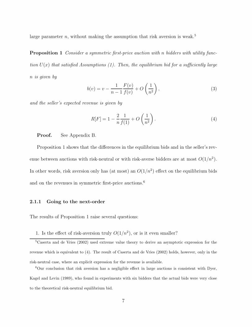
large parameter n, without making the assumption that risk aversion is weak.5

Proposition 1 Consider a symmetric first-price auction with n bidders with utility func-

tion U(x) that satisfied Assumptions (1). Then, the equilibrium bid for a sufficiently large

n is given by

b(v) = v − 1

n − 1

F (v)

f(v)+ O

(1

n2

), (3)

and the seller’s expected revenue is given by

R[F ] = 1 − 2

n

1

f(1)+ O

(1

n2

). (4)

Proof. See Appendix B.

Proposition 1 shows that the differences in the equilibrium bids and in the seller’s rev-

enue between auctions with risk-neutral or with risk-averse bidders are at most O(1/n2).

In other words, risk aversion only has (at most) an O(1/n2) effect on the equilibrium bids

and on the revenues in symmetric first-price auctions.6

2.1.1 Going to the next-order

The results of Proposition 1 raise several questions:

1. Is the effect of risk-aversion truly O(1/n2), or is it even smaller?

5Caserta and de Vries (2002) used extreme value theory to derive an asymptotic expression for the

revenue which is equivalent to (4). The result of Caserta and de Vries (2002) holds, however, only in the

risk-neutral case, where an explicit expression for the revenue is available.6Our conclusion that risk aversion has a negligible effect in large auctions is consistent with Dyer,

Kagel and Levin (1989), who found in experiments with six bidders that the actual bids were very close

to the theoretical risk-neutral equilibrium bid.

7

2. Can we estimate the constants in the O(1/n2) error terms?

3. To what extent do the results depend on Assumptions (1) for the utility function?

We can answer the first two questions by calculating explicitly the O(1/n2) terms:

Proposition 2 Consider a symmetric first-price auction with n bidders with utility func-

tion U(x) that satisfied Assumptions (1). Then, the equilibrium bid for a sufficiently

large n is given by

b(v) = v − 1

n − 1

F (v)

f(v)+

1

(n − 1)2

[F (v)

f(v)− F 2(v)f ′(v)

f3(v)− F 2(v)

2f2(v)

U ′′(0)

U ′(0)

]+ O

(1

n3

), (5)

and the seller’s expected revenue is given by

R[F ] = 1 − 1

n

2

f(1)+

1

n2

[2

f(1)− 3f ′(1)

f3(1)− 1

2f2(1)

U ′′(0)

U ′(0)

]+ O

(1

n3

). (6)

Proof. See Appendix C.

We thus see that risk-aversion has an O(1/n2) effect on the bid when U ′′(0) 6= 0, but a

smaller effect if U ′′(0) = 0. As expected, the bids and revenue increase (decrease) for risk-

averse (risk-loving) bidders. Note that the magnitude of risk-aversion effect is determined

by the value of the absolute risk-aversion −U ′′/U ′ at zero.

To answer the third question, we note that Assumptions (1) imply that U ′(0) < ∞,

and are thus invalid in the case of a CRRA utility function U(x) = xα, 0 < α < 1. In

that case, risk-aversion turns out to have an O(1/n) effect on the bid and revenue:

8

Lemma 1 Consider a large symmetric first-price auction with n bidders with a CRRA

utility function U(x) = xα where 0 < α < 1. Then,

b(v) = v − α

n

F (v)

f(v)+ O

(1

n2

), (7)

R[F ] = 1 − 1

n

1 + α

f(1)+ O

(1

n2

). (8)

Proof. See Appendix D.

The observation that risk-aversion has a small effect on the revenue in large auctions

is not surprising. Indeed, since in large auctions the bids are close to the values, one can

approximate U(v−b) ≈ (v−b)U ′(0), which is the risk-neutral case. However, this intuitive

argument cannot tell us that the effect of risk-aversion decays as 1/n2 when U ′(0) > 0,

but as 1/n for CRRA bidders, etc.

2.2 k-price auctions

The results of Proposition 1 can be generalized to any k-price auction:7

Proposition 3 Consider a symmetric k-price auction (k = 1, 2, 3, . . . ), with n bidders

with utility function U(x) that satisfies Assumptions (1). Then, the equilibrium bid for a

sufficiently large n is

b(v) = v +k − 2

n − k

F (v)

f(v)+ O

(1

n2

), (9)

and the seller’s expected revenue is given by (4).

7In a k-price auction the bidder with the highest bid wins the auction and pays the k-th highest bid.

For more details on k-price auctions with risk averse bidders, see Monderer and Tennenholtz (2000).

9

Proof. See Appendix E.

Recall that in the risk-neutral case U(x) = x, the equilibrium bids in k-price auctions

are given by (Wolfstetter, 1995)

b(v) = v +k − 2

n − k + 1

F (v)

f(v).

Comparison with equation (9) shows that in large symmetric k-price auctions, risk aversion

only has an O(1/n2) effect on the equilibrium bids. Proposition 3 also shows that risk

aversion only has an O(1/n2) effect on the revenue in large symmetric k-price auctions.

Since all k-price auctions are revenue equivalent in the risk-neutral case, this implies,

in particular, that all large symmetric k-price auctions, with risk-loving or risk-averse

bidders, are O(1/n2) revenue equivalent.

Remark. As in the case of first-price auctions (see Section 2.1.1), we can calculate

explicitly the O(1/n2) terms in order to to see that the effect of risk-aversion is truly

O(1/n2) when U ′(0) > 0 and U ′′(0) 6= 0, that the effect of risk-aversion is only O(1/n) for

CRRA bidders, etc.

3 Asymmetric large auctions

We now consider the case of large asymmetric auctions with n risk-neutral bidders. The

valuation of bidder i for the object vi is independently distributed according to a distribu-

tion function Fi(v) on the common interval [0, 1]. We denote by fi = F ′i the corresponding

density function.

10

We assume that fj , f ′j and f ′′

j are uniformly bounded, i.e., that there exist two positive

constants 0 < m < M , such that for every v ∈ [0, 1] and for j = 1, . . . , n,

m ≤ fj(v) ≤ M, |f ′j(v|), |f ′′

j (v)| ≤ M. (10)

In fact, for our results to hold, it is enough to require that (10) holds in a small neighbor-

hood of v = 1.

We denote by

FG(v) =

(n∏

i=1

Fi(v)

)1/n

the geometric average of the distribution functions and also denote fG(v) = F ′G(v).

3.1 Second-price auctions

Consider a large number (n � 1) of asymmetric bidders with distribution functions

F1, . . . , Fn who are competing for a single object in a second-price auction. In this case,

the equilibrium bid functions are bi(v) = v, and the seller’s expected revenue is given by

(see, e.g., Fibich and Gavious (2003))

R2nd[F1, . . . , Fn] = 1 −∫ 1

0

n∏

i=1

Fi(v) dv −n∑

i=1

∫ 1

0

(1 − Fi(v))n∏

j=1j 6=i

Fj(v) dv. (11)

Asymptotic expansion of R2nd in 1/n leads to the following result:

Proposition 4 In an asymmetric large second-price auction with n bidders, the seller’s

expected revenue for a sufficiently large n is

R2nd[F1, . . . , Fn] = 1 − 2

n

1

fG(1)+ O

(1

n2

), (12)

11

where fG(1) = F ′G(1) = 1

n

n∑j=1

fj(1).

Proof. See Appendix F.

Cantillon (2003) showed that the revenue in asymmetric second-price auctions is al-

ways smaller than in a symmetric second-price auctions with the same number of players

whose (symmetric) distribution function is FG. Since fG(1) is the same in both cases,

Proposition 4 shows that the revenue difference between the two cases is O(1/n2) small.

Example 1 We consider a large asymmetric second-price auction where bidders are equally

split to n/2 bidders with a distribution function F1(v) = v1/2 and n/2 bidders with a dis-

tribution function F2(v) = v2.

In this case, 1fG(1)

= 4/5 and the asymptotic approximation (12) yields

R2nd = 1 − 8

5n+ O

(1

n2

). (13)

By (11), the exact value of the seller’s expected revenue is given by

R2nd = 1 +n − 1

1.25n + 1− n/2

1.25n − 1− n/2

1.25n + 0.5.

Expanding this in 1/n gives

R2nd = 1 − 8

5n+

104

125n2+ . . . ,

which is in agreement with (13).

12

3.2 Asymptotic revenue equivalence

In the following we show that the asymptotic expression for the revenue in asymmetric

second-price auctions (12) can be generalized to a large class of asymmetric auctions.8

Theorem 1 Consider any auction mechanism that satisfies the following conditions:

1. All n players are risk neutral.

2. Player i’s valuation is private information to i and is drawn independently by a twice

continuously differentiable distribution function Fi(v) from a support [0, 1].

3. The object is allocated to the player with the highest bid.9

4. Any player with valuation 0 expects zero surplus.

5. The maximal bid is identical for all bidders, i.e., bi(1) = bj(1) for every i and j.10

6. The asymmetry among the equilibrium bids and their first, second, and third deriva-

tives at the maximal value is at most O(1/n), i.e., b(k)i (1)/b

(k)j (1) = 1 + O(1/n) for

every i and j, and for k = 1, 2, 3. 11

8Fibich, Gavious and Sela (2003) showed that weakly-asymmetric auctions are asymptotically revenue

equivalent, by expanding the revenue in the small asymmetry parameter. The result here is stronger,

since we do not need to assume that the asymmetry among players is weak.9In the symmetric case, assumption 3 is equivalent to the assumption that in equilibrium the object

is allocated to the player with the highest valuation. This equivalence, however, does not hold in the

asymmetric case since asymmetric auctions are not necessarily efficient.10This condition is satisfied e.g., for asymmetric first- and second price auctions.11The motivation for this condition is as follows. Since the environment (competition) that players i

13

Then, the seller’s expected revenue for a sufficiently large n is given by

R[F1, . . . , Fn] = 1 − 2

n

1

fG(1)+ O

(1

n2

). (14)

Proof. See Appendix G.

As we have said, previous studies established the revenue equivalence of a large class of

auctions in the limit as n −→ ∞. The novelty in Theorem 1 is, thus, in showing that the

O(1/n) deviation from the limiting value is also independent of the auction mechanism.

Clearly, in the case of symmetric auctions, the asymptotic relation (14) reduces to (4).

It is interesting to note that Condition 6 is not satisfied by asymmetric first-price auc-

tions, since in that case b′i(1)/b′j(1) = fi(1)/fj(1). Nevertheless, the result of Theorem 1

does hold for asymmetric first-price auctions, as is corroborated by our subsequent nu-

merical examples. The reason for this is that one can split the integration segment [0, 1]

into two segments [0, 1−ε] and [1−ε, 1], and choose ε = ε(n) � 1, such that Condition 6

holds for v = 1− ε, and such that the contribution of the interval [1− ε, 1] to the revenue

is O(1/n2). Therefore, application of Theorem 1 to the interval [0, 1 − ε] will yield the

result.

In order to examine the level of revenue equivalence when the number of players is

not really large, in Table 1 we compare the expected revenue in first-price auctions, the

expected revenue in second-price auction, and the asymptotic approximation for the rev-

enue, for the case of 6 asymmetric bidders with various distributions. The first thing to

and j face differs by one out of n− 1 players (i is facing j but not i and vice versa), one could expect the

resulting asymmetry among the bids to be O(1/n).

14

note is that our asymptotic prediction

R[F1, . . . , Fn] ≈ 1 − 2

n

1

fG(1)= 1 − 2∑n

i=1 fi(1)

is considerably more accurate12 than the ‘old’ prediction

R[F1, . . . , Fn] ≈ limn→∞

R[F1, . . . , Fn] = 1.

In addition, the good agreement between the asymptotic prediction and the actual rev-

enues suggests (yet again) that the results of the asymptotic analysis are already valid

for n ≈ 6. Finally, we note that in all cases the differences between R1st and R2nd are

only in the fourth or fifth digit. This observation suggests that, for all practical purposes,

first-price and second-price auction with n ≥ 6 bidders are revenue equivalent.

distributions R1st R2nd 1 − 2n

1fG(1)

R1st − R2nd R1st −(1 − 2

n1

fG(1)

)

F1 = F2 = F3 = F4 = v4, F5 = F6 = v1/2 0.877782 0.877778 0.882353 0.000004 -0.004571

F1 = F2 = F3 = v4, F4 = F5 = F6 = v1/2 0.84487 0.84483 0.851852 0.00004 -0.006982

F1 = F2 = F3 = v2, F4 = F5 = F6 = v1/2 0.751773 0.751697 0.733333 0.00008 0.01844

Fi = vi, i = 1, . . . , 6 0.900224 0.900143 0.904762 0.000081 -0.004538

Table 1: Expected revenue R1st[F1, . . . , F6] and R2nd[F1, . . . , F6].

4 Concluding remarks

Fibich, Gavious and Sela (2003) showed that for weakly-asymmetric auction, if ε is the

small asymmetry parameter, all standard auctions are O(ε2) revenue equivalent. Hence,

12by a factor of 13–27 for these examples

15

the revenue difference among weakly-asymmetric auctions is negligible. In this study

we do not assume that the asymmetry is weak, yet we find that the revenue difference

among large asymmetric auctions is also negligible. Together, these two studies suggest

that in most cases asymmetry among bidders valuations plays a minor role in revenue

ranking of auctions. Since asymmetry leads to a considerable increase in the complexity

of the mathematical model, but has negligible effect on revenue ranking, it can probably be

neglected in revenue ranking studies. A similar conclusion, however, cannot be applied to

risk-aversion. Indeed, Fibich, Gavious and Sela (2002) showed that for symmetric auction

with weakly-risk averse bidders, if ε is a small risk-aversion parameter, risk aversion has

an O(ε) effect on the equilibrium bids, and then the revenue difference among auctions

is O(ε). Therefore, risk-aversion can play an important role in revenue ranking of small

auctions, but not in large ones.

If we try to generalize the results of this research, we can identify several unifying

themes: 1) Auctions with a large number of bidders are considerably simpler to analyze

than auctions with a small number of bidders, since the effects of various “complications”

such as asymmetry, and risk-aversion are negligible. 2) The revenue ranking of large

auctions is more of academic than of practical value. 3) Auctions with as few as six

bidders can be considered as large auctions.

The last point raises the important question of how large the number of bidders (n)

should be for our asymptotic results to be valid. Since our expansions have an O(1/n2)

accuracy, roughly speaking, they have a 1% accuracy for 10 bidders. As the numerical

examples in this study show, however, our asymptotic results are already quite accurate

16

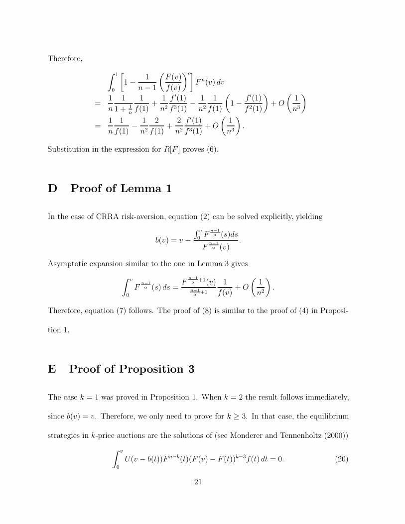
even for values as low as n = 6. The issue of how small can n be for our asymptotic results

to be valid can be resolved theoretically, in principle, by calculating explicitly the next

O(1/n2) term in the asymptotic expansion, but this is beyond the scope of the present

study.

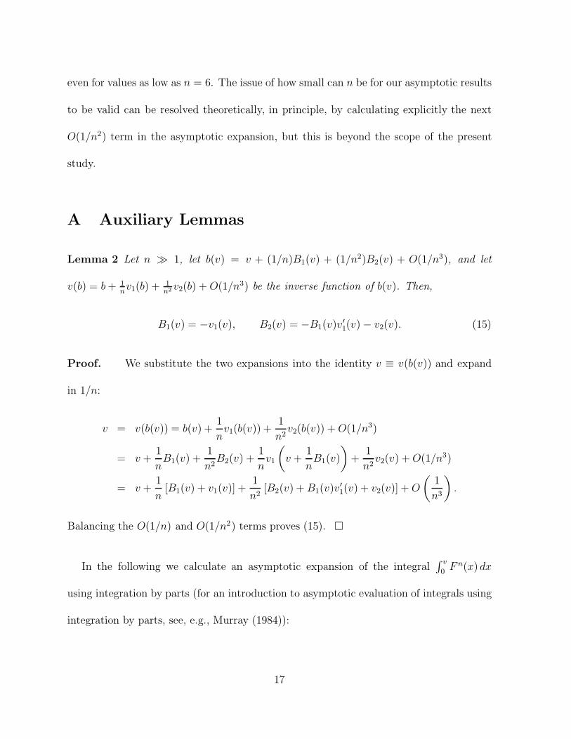
A Auxiliary Lemmas

Lemma 2 Let n � 1, let b(v) = v + (1/n)B1(v) + (1/n2)B2(v) + O(1/n3), and let

v(b) = b + 1nv1(b) + 1

n2 v2(b) + O(1/n3) be the inverse function of b(v). Then,

B1(v) = −v1(v), B2(v) = −B1(v)v′1(v) − v2(v). (15)

Proof. We substitute the two expansions into the identity v ≡ v(b(v)) and expand

in 1/n:

v = v(b(v)) = b(v) +1

nv1(b(v)) +

1

n2v2(b(v)) + O(1/n3)

= v +1

nB1(v) +

1

n2B2(v) +

1

nv1

(v +

1

nB1(v)

)+

1

n2v2(v) + O(1/n3)

= v +1

n[B1(v) + v1(v)] +

1

n2[B2(v) + B1(v)v′

1(v) + v2(v)] + O

(1

n3

).

Balancing the O(1/n) and O(1/n2) terms proves (15). �

In the following we calculate an asymptotic expansion of the integral∫ v

0F n(x) dx

using integration by parts (for an introduction to asymptotic evaluation of integrals using

integration by parts, see, e.g., Murray (1984)):

17

Lemma 3 Let F (v) be a twice-continuously differentiable, function and let f = F ′ > 0.

Then, for a sufficiently large n,

∫ v

0

F n(x) dx =1

n

F n+1(v)

f(v)

[1 + O

(1

n

)]. (16)

Proof. Using integration by parts,

∫ v

0

F n(x) dx =

∫ v

0

[F n(x)f(x)]1

f(x)dx =

1

n + 1

F n+1(v)

f(v)+

1

n + 1

∫ v

0

[F n+1(x)f(x)]f ′(x)

f3(x)dx

=1

n + 1

F n+1(v)

f(v)+

1

n + 1

1

n + 2F n+2(v)

f ′(v)

f3(v)− 1

n + 1

1

n + 2

∫ v

0

F n+2(x)

(f ′(x)

f3(x)

)′

dx.

Therefore, the result follows.

B Proof of Proposition 1

Since limn→∞ v(b) = b, we can look for a solution of (2) of the form

v(b) = b +1

n − 1v1(b) + O

(1

n2

).

Substitution in (2) gives

1 + O

(1

n

)

=1

n − 1

F (b) + (v1/(n − 1))f(b) + O(n−2)

f(b) + (v1/(n − 1))f ′(b) + O(n−2)· U ′(0) + (v1/(n − 1))U ′′(0) + O(n−2)

U(0) + (v1/(n − 1))U ′(0) + O(n−2).

Since U(0) = 0 and U ′(0) > 0, the balance of the leading order terms gives

1 =F (b)

f(b)· U ′(0)

v1U ′(0).

Therefore, v1(b) = F (b)/f(b) and the inverse equilibrium bids are given by

v(b) = b +1

n − 1

F (b)

f(b)+ O

(1

n2

).

18

Inverting this relation (see Lemma 2) shows that the equilibrium bids are given by (3).

To calculate the expected revenue, we use (3) to obtain

R[F ] =

∫ 1

0

b(v) dF n(v) = b(1) −∫ 1

0

b′(v)F n(v) dv

= 1 − 1

n

1

f(1)+ O

(1

n2

)−∫ 1

0

[1 + O(1/n)]F n(v) dv.

Therefore, by (16), the result follows.

C Proof of Proposition 2

Since limn→∞ v(b) = b, we can look for a solution of the form

v(b) = b +1

n − 1v1(b) +

1

(n − 1)2v2(b) + O

(1

n3

). (17)

Substituting (17) in (2) and using U(0) = 0 and 0 < U ′(0) < ∞ gives

1 +1

n − 1v′

1(b) + O

(1

n2

)

=1

n − 1

F (b) + v1

n−1f(b) + O(n−2)

f(b) + v1

n−1f ′(b) + O(n−2)

· U ′(0) + (v1/(n − 1))U ′′(0) + O(n−2)

U(0) + ( v1

n−1+ v2

(n−1)2)U ′(0) +

v21

2(n−1)2U ′′(0) + O(n−3)

=F (b) + v1

n−1f(b) + O(n−2)

f(b) + v1

n−1f ′(b) + O(n−2)

·U ′(0) + v1

n−1U ′′(0) + O(n−2)

(v1 + v2

(n−1))U ′(0) +

v21

2(n−1)U ′′(0) + O(n−2)

=

(F (b)

f(b)+

v1

n − 1+ O(n−2)

)(1 − v1

n − 1

f ′(b)

f(b)+ O(n−2)

)×

(1

v1+

1

n − 1

U ′′(0)

U ′(0)+ O(n−2)

)(1 − 1

(n − 1)

v2

v1− v1

2(n − 1)

U ′′(0)

U ′(0)+ O(n−2)

)

=F (b)

f(b)

1

v1+

1

n − 1

[1 − f ′(b)F (b)

f2(b)+

F (b)

2f(b)

U ′′(0)

U ′(0)− F (b)

f(b)

v2

v21

]+ O(n−2).

Balancing the O(1) terms gives, as before,

v1(b) =F (b)

f(b). (18)

19

Balancing the O( 1n−1

) terms gives

v′1(b) = 1 − f ′(b)F (b)

f2(b)+

F (b)

2f(b)

U ′′(0)

U ′(0)− F (b)

f(b)

v2

v21

.

Substituting v1(b) = F (b)/f(b) and v′1(b) = 1 − F (b)f ′(b)

f2(b)gives

v2(b) =F 2(b)

2f2(b)

U ′′(0)

U ′(0). (19)

Using Lemma 2 and (18,19) to invert the expansion (17) gives

b(v) = v +1

n − 1B1(v) +

1

(n − 1)2B2(v) + O

(1

n3

),

where

B1(v) = −F (v)

f(v), B2(v) =

F (v)

f(v)− F 2(v)f ′(v)

f3(v)− F 2(v)

2f2(v)

U ′′(0)

U ′(0).

This completes the proof of (5).

To calculate the expected revenue, we first use (5) to obtain

R[F ] =

∫ 1

0

b(v) dF n(v) = b(1) −∫ 1

0

b′(v)F n(v) dv

= 1 − 1

n − 1

1

f(1)+

1

(n − 1)2

[1

f(1)− f ′(1)

f3(1)− 1

2f2(1)

U ′′(0)

U ′(0)

]

−∫ 1

0

[1 − 1

n − 1

(F (v)

f(v)

)′]F n(v) dv + O

(1

n3

).

Integration by integration by parts (as in Lemma 3) gives,

∫ 1

0

F n(v) dv =1

n + 1

1

f(1)+

1

n + 1

1

n + 2

f ′(1)

f3(1)+ O

(1

n3

),

and∫ 1

0

(F (v)

f(v)

)′

F n(v) dv =1

n + 1

1

f(1)

(F (v)

f(v)

)′

v=1

+ O

(1

n2

).

20

Therefore,

∫ 1

0

[1 − 1

n − 1

(F (v)

f(v)

)′]F n(v) dv

=1

n

1

1 + 1n

1

f(1)+

1

n2

f ′(1)

f3(1)− 1

n2

1

f(1)

(1 − f ′(1)

f2(1)

)+ O

(1

n3

)

=1

n

1

f(1)− 1

n2

2

f(1)+

2

n2

f ′(1)

f3(1)+ O

(1

n3

).

Substitution in the expression for R[F ] proves (6).

D Proof of Lemma 1

In the case of CRRA risk-aversion, equation (2) can be solved explicitly, yielding

b(v) = v −∫ v

0F

n−1α (s)ds

Fn−1

α (v).

Asymptotic expansion similar to the one in Lemma 3 gives

∫ v

0

Fn−1

α (s) ds =F

n−1α

+1(v)n−1

α+1

1

f(v)+ O

(1

n2

).

Therefore, equation (7) follows. The proof of (8) is similar to the proof of (4) in Proposi-

tion 1.

E Proof of Proposition 3

The case k = 1 was proved in Proposition 1. When k = 2 the result follows immediately,

since b(v) = v. Therefore, we only need to prove for k ≥ 3. In that case, the equilibrium

strategies in k-price auctions are the solutions of (see Monderer and Tennenholtz (2000))

∫ v

0

U(v − b(t))F n−k(t)(F (v)− F (t))k−3f(t) dt = 0. (20)

21

Defining m = n − k and t = v − s, we can rewrite equation (20) as

0 =

∫ v

0

U(v − b(t))F m(t)(F (v)− F (t))k−3f(t) dt (21)

=

∫ v

0

em ln(F (t))U(v − b(t))(F (v)− F (t))k−3f(t) dt

= em lnF (v)

∫ v

0

e−m[ln F (v)−lnF (v−s)] U(v − b(v − s))(F (v)− F (v − s))k−3f(v − s) ds.

Since the maximum of ln(F (v − s)) is attained at s = 0, we can calculate an asymptotic

approximation of this integral using Laplace method (see, e.g., Murray (1984)). To do

that, we make the change of variables x(s) = [lnF (v) − lnF (v − s)] and expand all the

terms in the last integral in a Taylor series in s near s = 0.

Expansion of x(s) near s = 0 gives x = sf(v)/F (v) + O(s2). Therefore,

dx

ds= f(v)/F (v) + O(s), s = x

F (v)

f(v)+ O(s2), ds =

dx

f(v)/F (v)[1 + O(x)]

Let us expand the solution b(v) in a power series in m, i.e.,

b(v) = b0(v) +1

mb1(v) + O

(1

m2

).

Therefore, near s = 0,

b(v − s) = b0(v)− sb′0(v) +1

mb1(v)− 1

msb′1(v) + O(s2) + O

(1

m2

).

In addition,

(F (v)− F (v − s))k−3 = (sf(v) + O(s2))k−3 = sk−3fk−3(v)1 + O(s)],

and

f(v − s) = f(v) + O(s).

22

Substitution all the above in (21) gives

0 =

∫ v

0

{e−mx U

[v −

(b0(v)− sb′0(v) +

b1(v)

m− sb′1(v)

m+ O(s2) + O

(1

m2

))]×

sk−3fk−3(v) [1 + O(s)] [f(v) + O(s)]

}ds

∼∫ ∞

0

{e−mx U

[v −

(b0(v)− x

F (v)

f(v)b′0(v) +

1

mb1(v) − x

m

F (v)

f(v)b′1(v) + O(x2) + O

(1

m2

))]×

xk−3F k−3(v) [1 + O(x)] [f(v) + O(x)]dx

f(v)/F (v)[1 + O(x)]

}

= F k−2(v)

∫ ∞

0

{e−mx

[U(v − b0(v)) + U ′(v − b0(v))

(xF (v)

f(v)b′0(v) − b1(v)

m+

x

m

F (v)

f(v)b′1(v)

)

+O(x2) + O

(1

m2

)]xk−3 [1 + O(x)]

}dx. (22)

We recall that for p integer,∫∞

0e−mxxp dx = p!/mp+1. Therefore, balancing the leading

O(m−(k−2)) terms gives

U(v − b0(v))F k−2(v)

∫ ∞

0

e−mx xk−3 dx = 0.

Since U(z) = 0 only at z = 0, this implies that b0(v) ≡ v. Using this and U ′(0) = 0,

equation (22) reduces to

0 =

∫ ∞

0

{e−mx

(xF (v)

f(v)− 1

mb1(v) +

x

m

F (v)

f(v)b′1(v)

)[xk−3 + O(xk−2)

]}dx

Therefore, balance of the next-order O(m−(k−1)) terms gives

F (v)

f(v)

∫ ∞

0

e−mxxk−2 dx − 1

mb1(v)

∫ ∞

0

e−mxxk−3 dx = 0,

or

F (v)

f(v)

(k − 2)!

mk−1− (k − 3)!

mk−1b1(v) = 0.

Therefore,

b1(v) = (k − 2)F (v)

f(v).

23

Hence, we proved (9).

The seller’s expected revenue in a k-price auction is given by

Rk =

∫ 1

0

b(v)dFk(v),

where b(v) is the equilibrium bid in the k price auction and Fk(v) is the distribution

of the k-th valuation in order (i.e., k-order statistic of the bidders private valuations).

Substituting the asymptotic expansion for the equilibrium bids gives

Rk =

∫ 1

0

[v +

k − 2

n − k

F (v)

f(v)

]dFk(v) + O(

1

n2).

Since the asymptotic expansion for the equilibrium bid is independent of the utility func-

tion U until order O( 1n2 ), the revenue in the risk-averse case is the same as in the risk-

neutral case, with O( 1n2 ) accuracy. By the revenue equivalence theorem, the latter is given

by (4).

F Proof of Proposition 4

From (11) it follows that

R2nd[F1, . . . , Fn] = 1 −∫ 1

0

n∏

i=1

Fi(v) dv −n∑

i=1

∫ 1

0

(1 − Fi(v))

Fi(v)

n∏

j=1

Fj(v) dv. (23)

Repeating the proof of Lemma 3 with F = FG gives

∫ 1

0

n∏

i=1

Fi(v) dv =

∫ 1

0

F nG(v) dv =

1

n + 1

1

fG(1)− 1

n + 1

1

n + 2

1

fG(1)

(1

fG

)′ ∣∣∣∣v=1

+1

n + 1

1

n + 2

∫ 1

0

F n+2G (v)

(1

fG(v)

(1

fG(v)

)′)′

dv.

24

Since 1/fG(1), (1/fG)′|v=1 and∫ 1

0F n+2

G (v)

(1

fG(v)

(1

fG(v)

)′)′

dv are uniformly bounded

in n, see Lemma 4,∫ 1

0

n∏

i=1

Fi(v) dv =1

n

1

fG(1)+ O

(1

n2

). (24)

In order to continue to evaluate the remaining terms in (23), we first use two integra-

tions by parts

∫ 1

0

(1 − Fi(v))

Fi(v)

n∏

j=1

Fj(v) dv

=1

n + 1

F n+1G (v)

fG(v)

1 − Fi(v)

Fi(v)

∣∣∣∣1

0

− 1

n + 1

∫ 1

0

F n+1G (v)

fG(v)

fG(v)

(1

fG(v)

1 − Fi(v)

Fi(v)

)′

dv

= 0 − 1

n + 1

1

n + 2

F n+2G (v)

fG(v)

(1

fG(v)

1 − Fi(v)

Fi(v)

)′∣∣∣∣1

0

+1

n + 1

1

n + 2

∫ 1

0

F n+2G (v)

(1

fG(v)

(1

fG(v)

1 − Fi(v)

Fi(v)

)′)′

dv

=1

n2

fi(1)

f2G(1)

+1

n2

∫ 1

0

F n+2G (v)

(1

fG(v)

(1

fG(v)

1 − Fi(v)

Fi(v)

)′)′

dv + O

(1

n3

).

Arguments similar to the ones in Lemma 4 show that F 3G(v)

(1

fG(v)

(1

fG(v)1−Fi(v)Fi(v)

)′)′

is

uniformly bounded. Therefore,

∣∣∣∣∫ 1

0

F n+2G (v)

(1

fG(v)

(1

fG(v)

1 − Fi(v)

Fi(v)

)′)′

dv

∣∣∣∣ ≤ C

∫ 1

0

F n−1G (v) dv = O(1/n),

where is the last stage we used (24). Since, in addition, fG(1) = 1n

n∑i=1

fi(1),

n∑

i=1

∫ 1

0

(1 − Fi(v))

Fi(v)

n∏

j=1

Fj(v) dv =1

n2

n∑i=1

fi(1)

f2G(1)

+ O

(1

n2

)=

1

n

1

fG(1)+ O

(1

n2

).

Substituting the last relation and (24) in (23) concludes the proof.

Lemma 4 There exists a positive number C, independent of n, such that

|1/fG(1)| ≤ C, |(1/fG)′(1)| ≤ C,

∣∣∣∣∣

∫ 1

0

F n+2G (v)

(1

fG(v)

(1

fG(v)

)′)′

dv

∣∣∣∣∣ ≤ C.

25

Proof: From Assumptions (10) it follows that mv ≤ Fj(v) ≤ Mv. Therefore, mv ≤

FG(v) ≤ Mv, and

m

M≤ FG(v)

Fj(v)≤ M

m, 0 ≤ v ≤ 1. (25)

Since

fG(v) =1

nFG(v)

n∑

j=1

fj(v)

Fj(v)=

1

n

n∑

j=1

FG(v)

Fj(v)fj(v), (26)

equation (25) implies that

m2

M≤ fG(v) ≤ M2

m,

m

M2≤ 1

fG(v)≤ M

m2. (27)

In particular, we see that 1/fG(1) is uniformly bounded.

Differentiating equation (26) gives

f ′G(v) =

1

n2FG(v)

(n∑

j=1

fj(v)

Fj(v)

)2

+1

nFG(v)

n∑

j=1

f ′j(v)Fj(v)− f2

j (v)

F 2j (v)

. (28)

Therefore, from assumptions (10) it immediately follows that |f ′G(1)| is uniformly bounded,

hence also |(1/fG)′|v=1.

In order to bound the integral, we first note that since F nG(v) ≤ 1, it is enough to show

that

F 2G(v)

(1

fG(v)

(1

fG(v)

)′)′

= −F 2G(v)f ′′

G(v)

f3G(v)

+ 3F 2

G(f ′G(v))2

f4G(v)

is bounded (uniformly in v and in n). In light of (27), we only need to show that F 2Gf ′′

G

and FGf ′G are bounded. Indeed, by (28),

FG(v)f ′G(v) =

1

n2

(n∑

j=1

FG(v)

Fj(v)fj(v)

)2

+1

n

n∑

j=1

F 2G(v)

F 2j (v)

(f ′

j(v)Fj(v)− f2j (v)

).

26

Therefore, relations (10,27) show that |FG(v)f ′G(v)| is uniformly bounded. Similar argu-

ments show that

F 2G(v)f ′′

G(v) =1

n3

(n∑

j=1

FG(v)

Fj(v)fj(v)

)3

+3

n2

n∑

j=1

FG(v)fj(v)

Fj(v)

n∑

j=1

F 2G(v)

F 2j (v)

(f ′

j(v)Fj(v) − f2j (v)

)

+1

nFG(v)

n∑

j=1

F 2G(v)

F 2j (v)

(f ′′

j (v)Fj(v)− fj(v)f ′j(v)

)

−1

n

n∑

j=1

F 3G(v)

F 3j (v)

2(f ′

j(v)Fj(v)− f2j (v)

)fj(v)

is uniformly bounded.

G Proof of Theorem 1

When all players with a zero valuation expect a zero surplus (Condition 4), then the

seller’s expected revenue is given by (Fibich, Gavious and Sela, 2003)

R = −n∑

i=1

∫ v̄

v

Pi(v)[v(1− Fi(v))]′ dv, (29)

where Pi(v) is the probability of winning for bidder i with type v at equilibrium. Since

Pi(v) = P

(bi(v) > max

j 6=ibj

)=

n∏

j=1j 6=i

Fj(b−1j (bi(v))),

we can rewrite (29) as

R = −n∑

i=1

∫ 1

0

(n∏

j=1

Fj(b−1j (bi(v))

)1 − Fi(v) − vfi(v)

Fi(v)dv.

In order to approximate R for large n, we use an asymptotic method known as Laplace

method for integrals (see, e.g., Murray (1984)). We first define

Gi(v) =

(n∏

j=1

Fj(b−1j (bi(v))

)1/n

, gi(v) =d

dvGi(v).

27

Then, we have

R = −n∑

i=1

∫ 1

0

en lnGi(v) ·(

1 − Fi(v)− vfi(v)

Fi(v)

)dv

= −n∑

i=1

∫ 1

0

en lnGi(1−s) ·(

1 − Fi(1 − s) − (1 − s)fi(1 − s)

Fi(1 − s)

)ds, (30)

where the last equality is obtained by the change of variables s = 1 − v.

The essence of Laplace method is the realization that as n increases, the contribution to

each integral comes essentially only from the neighborhood of the point where Gi attains

its maximum, i.e., near v = 1 or s = 0. Hence, with exponential accuracy, one can

replace the integrand with its Taylor expansion near s = 0, and also extend the domain

of integration from [0, 1] to [0, ∞). To do that, let us first prove the following result:

Lemma 5 Let xi(s) = − lnGi(1 − s), and let 0 ≤ s � 1. Then,

s =xi

gi(1)(1 + O(xi)) , ds =

dxi

gi(1)

[1 + xi

(g′

i(1)

g2i (1)

− 1

)+ O(x2

i )

].

Proof. Taylor expansion in s gives13

xi = sgi(1) +s2

2η(z(s)), η(s) =

d

ds

(gi(1 − s)

Gi(1 − s)

), 0 ≤ z(s) ≤ s.

Solving the quadratic equation for s (for the root that satisfies x(s = 0) = 0) gives

s =−gi(1) +

√g2

i (1) + 2xiη

η,

Since xi � 1, and since |η(z(s))|, |1/gi(1)| ≤ C, see Lemma 6, we can expand this

expression as

s =−gi(1) + gi

√1 + 2xiη/g2

i (1)

η=

xi

gi(1)

(1 − xiη

2g2i (1)

+ . . .

)=

xi

gi(1)(1 + O(xi)) .

13Here we used Condition 5 to deduce that Gi(1) = 1.

28

Similarly,

ds

dxi

=Gi(1 − s)

gi(1 − s)=

1

gi(1)−s

g2i (1) − g′

i(1)

g2i (1)

+s2

2ξ(w(s)), ξ =

d2

ds2

(Gi(1 − s)

gi(1 − s)

), 0 ≤ w(s) ≤ s.

Since |ξ(w(s))| ≤ C, see Lemma 6,

ds =dxi

gi(1)

[1 + xi

(g′

i(1)

g2i (1)

− 1

)+ O(x2

i )

].

�

In addition,

1 − Fi(1 − s) − (1 − s)fi(1 − s)

Fi(1 − s)= −fi(1) − s(f2

i (1) − f ′i(1) − 2fi(1)) + O(s2)

= −fi(1) −xi

gi(1)(f2

i (1) − f ′i(1) − 2fi(1)) + O(x2

i ).

Substituting the above in (30) gives that

R =

∫ ∞

0

n∑

i=1

[e−nxi

(fi(1) +

xi

gi(1)(f2

i (1) − f ′i(1) − 2fi(1))

)(1 + xi

(g′

i(1)

g2i (1)

− 1

))+O(x2

i )

]dxi

gi(1).

Since xi is a dummy variable, we can rename xi = x. Therefore,

R =n∑

i=1

∫ ∞

0

{e−nx ·

(fi(1) +

x

gi(1)(f2

i (1) − f ′i(1) − 2fi(1))

)(1 + xi

(g′

i(1)

g2i (1)

− 1

))+ O(x2)

}dx

gi(1)

=n∑

i=1

1

gi(1)

∫ ∞

0

e−nx

(fi(1) + x

[1

gi(1)(f2

i (1) − f ′i(1) − 2fi(1)) + fi(1)

(g′

i(1)

g2i (1)

− 1

)]+ O(x2)

)dx

=n∑

i=1

fi(1)

gi(1)

∫ ∞

0

e−nx dx

+

n∑

i=1

1

gi(1)

[1

gi(1)(f2

i (1) − f ′i(1) − 2fi(1)) + fi(1)

(g′

i(1)

g2i (1)

− 1

)]∫ ∞

0

e−nxx dx + O(n−2).

29

We thus see that

R =1

n

n∑

i=1

fi(1)

gi(1)+

1

n2

n∑

i=1

1

g2i (1)

[(f2

i (1) − f ′i (1) − 2fi(1)) + fi(1)

g′i(1)

gi(1)

]

− 1

n2

n∑

i=1

fi(1)

gi(1)+ O(n−2). (31)

In order to calculate the first term on the right-hand-side of (31), we first note that

gi(v) =d

dv

(n∏

j=1

Fj(b−1j (bi(v))

)1/n

=1

n

(n∏

k=1

Fk(b−1k (bi(v))

)1/n−1 n∑

j=1

(n∏

k 6=j

Fk(b−1k (bi(v))

)fj(b

−1j (bi(v))

b′i(v)

b′j(b−1j (bi(v))

= Gi(v)1

nb′i(v)

n∑

j=1

fj(b−1j (bi(v))

Fj(b−1j (bi(v))

1

b′j(b−1j (bi(v))

. (32)

Since all bidders have the same maximal bid, then b−1j (bi(1)) = 1. Therefore,

gi(1) =b′i(1)

n

n∑

j=1

fj(1)

b′j(1). (33)

¿From this, it follows that

gi(1) = αb′i(1), (34)

where α is a constant which is independent of i, and hence that

1

n

n∑

i=1

fi(1)

gi(1)= 1. (35)

Differentiating (32) and using b−1j (bi(1)) = 1 gives

g′i(1) =

1

n2(b′i(1))

2

(n∑

j=1

fj(1)

b′j(1)

)2

+1

nb′′i (1)

n∑

j=1

fj(1)

b′j(1)

+1

nb′i(1)

n∑

j=1

(f ′

j(1)

b′j(1)−

f2j (1)

b′j(1)−

fj(1)b′′j (1)

(b′j(1))2

)b′i(1)

b′j(1)

= g2i (1) +

b′′i (1)

b′i(1)gi(1) +

1

nb′i(1)

n∑

j=1

(f ′

j(1)

b′j(1)−

f2j (1)

b′j(1)−

fj(1)b′′j (1)

(b′j(1))2

)b′i(1)

b′j(1). (36)

30

Multiplying by fi(1) and using (34) gives

fi(1)g′i(1) = fi(1)g

2i (1) + αb′′i (1)fi(1) +

1

nfi(1)g

2i (1)

n∑

j=1

(f ′

j(1)

g2j (1)

−f2

j (1)

g2j (1)

−αfj(1)b

′′j (1)

g3j (1)

).

Dividing by g3i (1) and summing gives

n∑

i=1

(fi(1)g

′i(1)

g3i (1)

)=

n∑

i=1

fi(1)

gi(1)︸ ︷︷ ︸

=n

+αn∑

i=1

b′′i (1)fi(1)

g3i (1)

+

(1

n

n∑

i=1

fi(1)

gi(1)

)

︸ ︷︷ ︸=1

n∑

j=1

(f ′

j(1)

g2j (1)

−f2

j (1)

g2j (1)

−αfj(1)b

′′j (1)

g3j (1)

).

Therefore,n∑

i=1

(fi(1)g

′i(1)

g3i (1)

+f2

i (1) − f ′i(1)

g2i (1)

)= n.

Substituting this and (35) in (31) gives

R = 1 − 2

n2

n∑

i=1

fi(1)

g2i (1)

+ O(n−2). (37)

Using (33) and Condition 6 gives that

gi(1) =1

n

n∑

j=1

fj(1) + O(1/n). (38)

Substitution in (37) gives (14).

Lemma 6 Let s � 1. Then, there exist a positive constant C, independent of n, such

that

|1/gi(1)| ≤ C, |η(z(s))| ≤ C, |ξ(w(s))| ≤ C.

Proof. From (33) and Assumptions ?? it follows that

m + O(1/n) ≤ |gi(1)| ≤ M + O(1/n). (39)

31

Since s � 1, it follows that z(s), w(s) � 1 and thus, it suffices to bound |η(t)| and |ξ(t)|

for t � 1. Now,

η(t) =−g′

i(1 − t)Gi(1 − t) + g2i (1 − t)

G2i (1 − t)

,

ξ(t) =−g3

i (1 − t)g′i(1 − t) − g′′

i (1 − t)g2i (1 − t)Gi(1 − t) + 2gi(1 − t) (g′

i)2 (1 − t)Gi(1 − t)

g4i (1 − t)

.

Therefore, we need to bound Gi(1 − t), gi(1 − t), g′i(1 − t), g′′

i (1 − t), 1/Gi(1 − t) and

1/gi(1 − t). Since Gi(1) = 1, and since gi(1) is bounded from above and away from zero

from below, see (39), it is enough to bound g′i(1) and g′′

i (1), since by continuity, the bound

is still valid for t � 1. Using (36), and the conditions b′i(1)/b′j(1) = 1 + O(1/n) and

b′′i (1)/b′′j (1) = 1 + O(1/n), gives that

g′i(1) = g2

i (1) +1

n

n∑

j=1

(f ′

j(1) − f2j (1)

)+ O(1/n). (40)

Similarly, using also the condition that b′′′i (1)/b′′′j (1) = 1 + O(1/n) gives

g′′i (1) = g3

i (1) +3

ngi(1)

n∑

j=1

(f ′

j(1) − f2j (1)

)+

+1

n

n∑

j=1

(f ′′

j (1) − 2fj(1)f′j(1) + f3

j (1))

+ O(1/n).

Therefore, Assumptions (10) imply that g′i(1) and g′′

i (1) are uniformly bounded.

32

References

[1] Bali V. and Jackson, M. (2001): “Asymptotic Revenue Equivalence in Auctions,”

Journal of Economic Theory, 106, 161-176.

[2] Cantillon, E. (2003), ”The Effect of Bidders Asymmetries on Expected Revenue in

Auctions”, mimeo, available at http://www.people.hbs.edu/ecantillon

[3] Caserta, S. and de Vries, C. (2002): “Auctions with Numerous Bidders,” mimeo.

[4] Fibich, G. and Gavious, A. (2003): “Asymmetric First-Price Auctions - A Perturba-

tion Approach,” Mathematics of Operations Research 28: 836-852.

[5] Fibich, G., Gavious, A. and Sela, A. (2004): “Revenue Equivalence in Asymmetric

Auctions,” Journal of Economic Theory 115: 309-321.

[6] Fibich, G., Gavious A. and Sela A. (2002): “All-pay auctions with risk-averse buyers,”

working paper. Available electronically at www.math.tau.ac.il/∼fibich

[7] Dyer D., Kagel J. H. and Levin D. (1989): “Resolving Uncertainty About the Number

of Bidders in Independent Private-Value Auctions: An Experimental Analysis”, Rand

Journal of Economics, Vol. 20, No. 2, pp. 268-279.

[8] Hong, H. and Shum, M. (2004): “Rates of information aggregation in common value

auctions”, Journal of Economic Theory, Vol. 116, No. 1, pp. 1-40.

[9] Jackson, M.O. and Kremer, I. (2004): “The Relationship between the Allocation of

Goods and a Seller’s Revenue”, Journal of Mathematical Economics, 40, 371-392.

33

[10] Jackson, M.O. and Kremer, I. (2005): “The Relevance of a Choice of Auction Format

in a Competitive Environment”, working paper.

[11] Kremer, I. (2002): “Information aggregation in common value auctions”, Economet-

rica, 70, 4, 1675-1682.

[12] Krishna, V. (2002): Auction Theory, Academic Press.

[13] Lebrun, B. (1999), “First Price Auctions and the Asymmetric N Bidder Case,” In-

ternational Economic Review, 40, 125-142.

[14] Marshall, R. C., Meurer, M. J., Richard, J.-F. and Stromquist, W. (1994): “Numer-

ical Analysis of Asymmetric First Price Auctions,” Games and Economic Behavior,

7, 193-220.

[15] Maskin, E., Riley, J. G. (1984): “Optimal Auctions with Risk Averse Buyers,” Econo-

metrica, 6, 1473-1518.

[16] Maskin, E. S. and Riley, J. G. (2000): “Equilibrium in Sealed High Bid Auctions,”

Review of Economic Studies, 67, 439-454.

[17] Maskin, E. S. and Riley, J. G. (2000): “Asymmetric auctions,” Review of Economic

Studies, 67, 413-438.

[18] Matthews, S. (1987): “Comparing auctions for risk averse buyers: a buyer’s point of

view,” Econometrica, 55, 636-646.

[19] Murray, J. D. (1984): Asymptotic Analysis, Springer-Verlag, New York.

34

[20] Myerson, R. B. (1981): “Optimal Auction Design,” Mathematics of Operations Re-

search, 6, 58-73.

[21] Monderer, D. and Tennenholtz, M. (2000): “K-Price Auctions,” Games and Eco-

nomic Behavior, 31, 220-244.

[22] Pesendorfer, W. and Swinkels, J. M. (1997): “The Loser’s Curse and Information

Aggregation in Common Value Auctions,”Econometrica, 65, 1247-1282.

[23] Riley, J. G. and Samuelson, W. F. (1981): “Optimal Auctions,” American Economic

Review, 71, 381-392.

[24] Rustichini, A., Satterthwaite, M.A. and Williams, S.R. (1994): “Convergence to

Efficiency in a Simple Market with Incomplete Information, ” Econometrica, 62,

1041-1063.

[25] Satterthwaite, M.A. and Williams, S.R. (1989): “The Rate of Convergence to Effi-

ciency in the Buyer’s Bid Double Auction as the Market Becomes Large, ” Review

of Economic Studies, 56, 477-498.

[26] Swinkels, J. M. (1999): “Asymptotic Efficiency for Discriminatory Private Value

Auctions,” Review of Economic Studies 66, 509-528.

[27] Swinkels, J. M. (2001): “Efficiency of Large Private Value Auctions,” Econometrica,

69, 37-68.

35

[28] Vickrey, W. (1961): “Counterspeculation, Auctions, and Competitive Sealed Ten-

ders,” Journal of Finance, 16, 8-37.

[29] Wilson, R. (1976): “A Bidding Model of Perfect Competition,” Review of Economic

Studies, 44, 511-518.

[30] Wolfstetter, E. (1995): “Third- and Higher-Price Auctions,” mimeo.

36