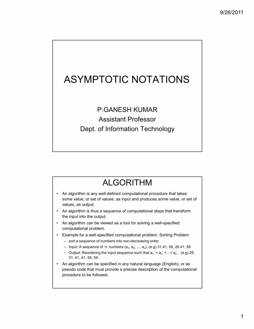
9/26/2011

1

ASYMPTOTIC NOTATIONS

P.GANESH KUMAR

Assistant Professor

Dept. of Information Technology

ALGORITHM• An algorithm is any well-defined computational procedure that takes

some value, or set of values, as input and produces some value, or set of

values, as output.

• An algorithm is thus a sequence of computational steps that transform

the input into the output.

• An algorithm can be viewed as a tool for solving a well-specified

computational problem.

• Example for a well-specified computational problem: Sorting Problem

– sort a sequence of numbers into non-decreasing order.

– Input: A sequence of ‘n’ numbers (a1, a2, ..., an), (e.g) 31,41, 59, 26,41, 58

– Output: Reordering the input sequence such that a1’ < a2’ <A< an’. (e.g) 26,

31, 41, 41, 58, 59.

• An algorithm can be specified in any natural language (English), or as

pseudo code that must provide a precise description of the computational

procedure to be followed.

9/26/2011

2

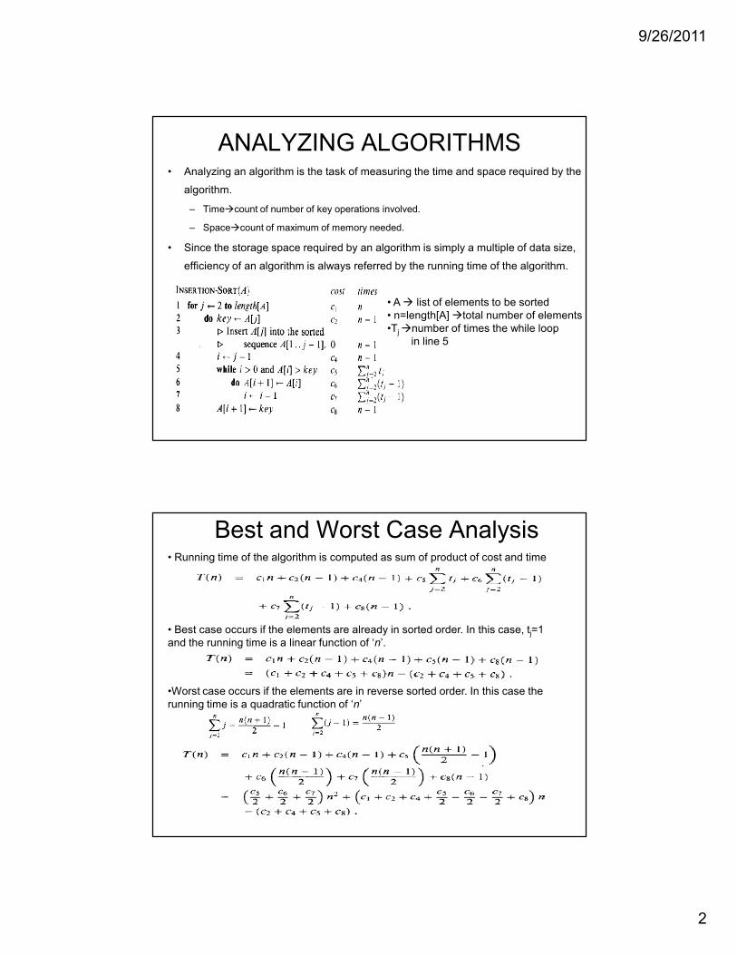
ANALYZING ALGORITHMS• Analyzing an algorithm is the task of measuring the time and space required by the

algorithm.

– Timecount of number of key operations involved.

– Spacecount of maximum of memory needed.

• Since the storage space required by an algorithm is simply a multiple of data size,

efficiency of an algorithm is always referred by the running time of the algorithm.

• A list of elements to be sorted

• n=length[A] total number of elements

•Tj number of times the while loop

in line 5

Best and Worst Case Analysis• Running time of the algorithm is computed as sum of product of cost and time

• Best case occurs if the elements are already in sorted order. In this case, tj=1

and the running time is a linear function of ‘n’.

•Worst case occurs if the elements are in reverse sorted order. In this case the

running time is a quadratic function of ‘n’

9/26/2011

3

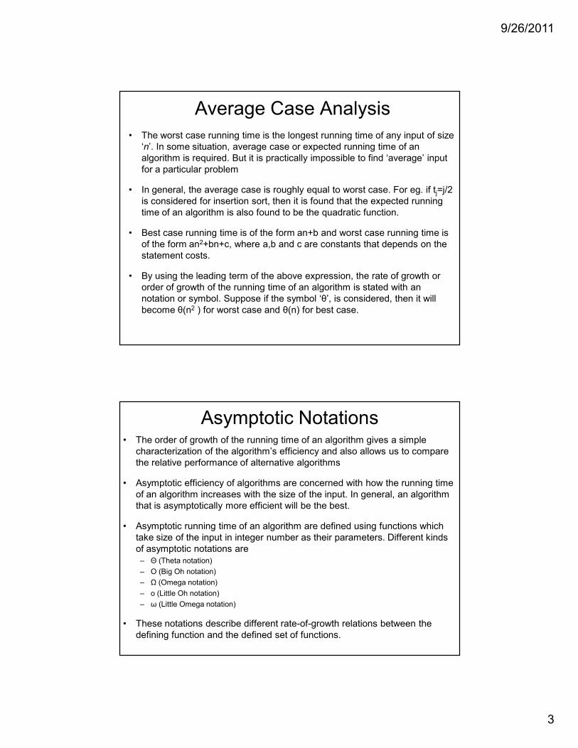
Average Case Analysis

• The worst case running time is the longest running time of any input of size

‘n’. In some situation, average case or expected running time of an

algorithm is required. But it is practically impossible to find ‘average’ input

for a particular problem

• In general, the average case is roughly equal to worst case. For eg. if tj=j/2

is considered for insertion sort, then it is found that the expected running

time of an algorithm is also found to be the quadratic function.

• Best case running time is of the form an+b and worst case running time is

of the form an2+bn+c, where a,b and c are constants that depends on the

statement costs.

• By using the leading term of the above expression, the rate of growth or

order of growth of the running time of an algorithm is stated with an

notation or symbol. Suppose if the symbol ‘θ’, is considered, then it will

become θ(n2 ) for worst case and θ(n) for best case.

Asymptotic Notations• The order of growth of the running time of an algorithm gives a simple

characterization of the algorithm’s efficiency and also allows us to compare

the relative performance of alternative algorithms

• Asymptotic efficiency of algorithms are concerned with how the running time

of an algorithm increases with the size of the input. In general, an algorithm

that is asymptotically more efficient will be the best.

• Asymptotic running time of an algorithm are defined using functions which

take size of the input in integer number as their parameters. Different kinds

of asymptotic notations are

– Θ (Theta notation)

– O (Big Oh notation)

– Ω (Omega notation)

– o (Little Oh notation)

– ω (Little Omega notation)

• These notations describe different rate-of-growth relations between the

defining function and the defined set of functions.

9/26/2011

4

7

Algorithm Analysis: Example

• Alg.: MIN (a[1], …, a[n])m ← a[1];

for i ← 2 to n

if a[i] < m

then m ← a[i];

• Running time:

– the number of primitive operations (steps)

executed before terminationT(n) =1 [first step] + (n) [for loop] + (n-1) [if condition] +

(n-1) [the assignment in then] = 3n - 1

• Order (rate) of growth:

– The leading term of the formula

– Expresses the asymptotic behavior of the algorithm

8

Typical Running Time Functions

• 1 (constant running time):

– Instructions are executed once or a few times

• logN (logarithmic)

– A big problem is solved by cutting the original problem in smaller

sizes, by a constant fraction at each step

• N (linear)

– A small amount of processing is done on each input element

• N logN

– A problem is solved by dividing it into smaller problems, solving

them independently and combining the solution

9/26/2011

5

9

Typical Running Time Functions

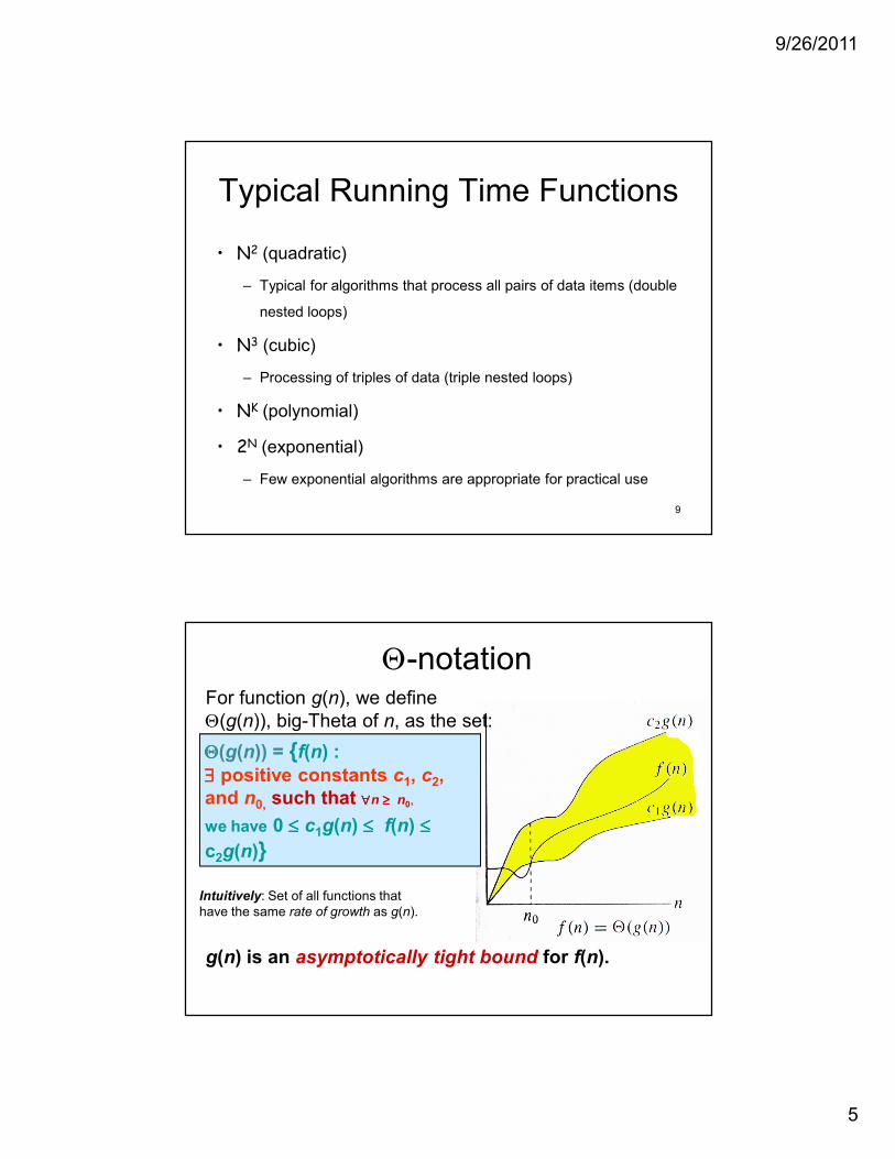
• N2 (quadratic)

– Typical for algorithms that process all pairs of data items (double

nested loops)

• N3 (cubic)

– Processing of triples of data (triple nested loops)

• NK (polynomial)

• 2N (exponential)

– Few exponential algorithms are appropriate for practical use

Θ-notation

ΘΘΘΘ(g(n)) = f(n) : ∃∃∃∃ positive constants c1, c2,

and n0, such that ∀∀∀∀n ≥≥≥≥ n0,

we have 0 ≤≤≤≤ c1g(n) ≤≤≤≤ f(n) ≤≤≤≤

c2g(n)

For function g(n), we define

Θ(g(n)), big-Theta of n, as the set:

g(n) is an asymptotically tight bound for f(n).

Intuitively: Set of all functions that

have the same rate of growth as g(n).

9/26/2011

6

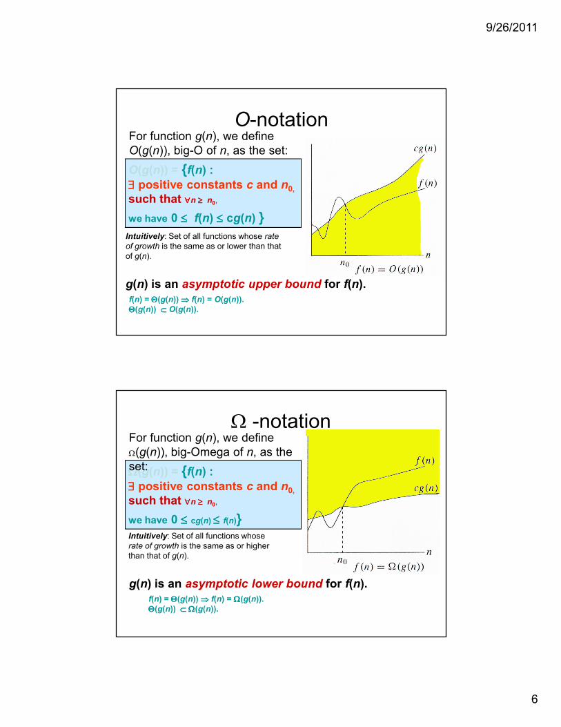
O-notation

O(g(n)) = f(n) : ∃∃∃∃ positive constants c and n0,such that ∀∀∀∀n ≥≥≥≥ n0,

we have 0 ≤≤≤≤ f(n) ≤≤≤≤ cg(n)

For function g(n), we define

O(g(n)), big-O of n, as the set:

g(n) is an asymptotic upper bound for f(n).

Intuitively: Set of all functions whose rate

of growth is the same as or lower than that

of g(n).

f(n) = ΘΘΘΘ(g(n)) ⇒⇒⇒⇒ f(n) = O(g(n)).

ΘΘΘΘ(g(n)) ⊂⊂⊂⊂ O(g(n)).

Ω -notation

g(n) is an asymptotic lower bound for f(n).

Intuitively: Set of all functions whose

rate of growth is the same as or higher

than that of g(n).

f(n) = ΘΘΘΘ(g(n)) ⇒⇒⇒⇒ f(n) = ΩΩΩΩ(g(n)).

ΘΘΘΘ(g(n)) ⊂⊂⊂⊂ ΩΩΩΩ(g(n)).

ΩΩΩΩ(g(n)) = f(n) : ∃∃∃∃ positive constants c and n0,such that ∀∀∀∀n ≥≥≥≥ n0,

we have 0 ≤≤≤≤ cg(n) ≤≤≤≤ f(n)

For function g(n), we define

Ω(g(n)), big-Omega of n, as the

set:

9/26/2011

7

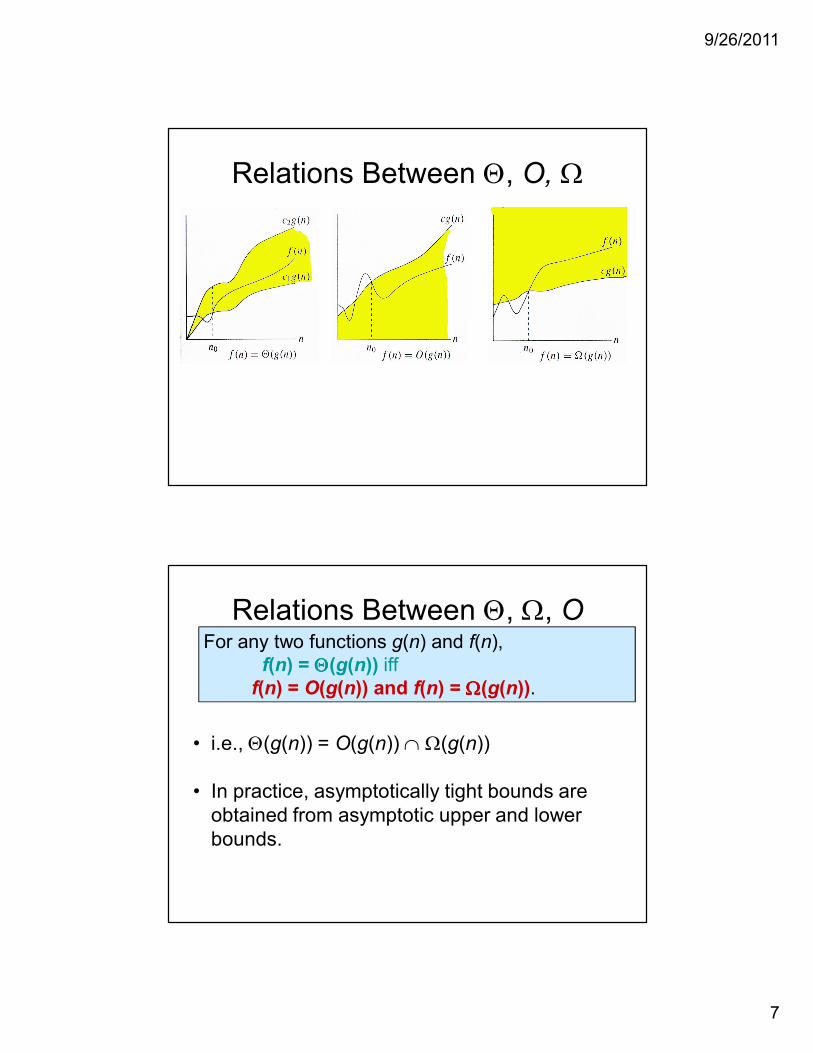
Relations Between Θ, O, Ω

Relations Between Θ, Ω, O

• i.e., Θ(g(n)) = O(g(n)) ∩ Ω(g(n))

• In practice, asymptotically tight bounds are

obtained from asymptotic upper and lower

bounds.

For any two functions g(n) and f(n),

f(n) = ΘΘΘΘ(g(n)) iff

f(n) = O(g(n)) and f(n) = ΩΩΩΩ(g(n)).

9/26/2011

8

15

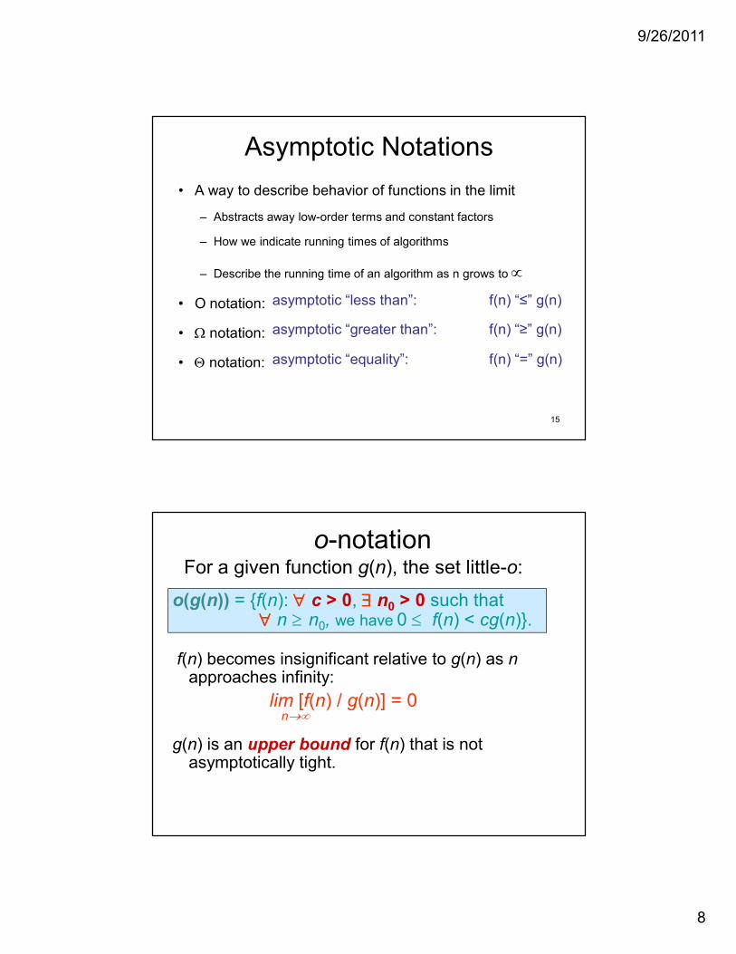
Asymptotic Notations

• A way to describe behavior of functions in the limit

– Abstracts away low-order terms and constant factors

– How we indicate running times of algorithms

– Describe the running time of an algorithm as n grows to ∝

• O notation:

• Ω notation:

• Θ notation:

asymptotic “less than”: f(n) “≤” g(n)

asymptotic “greater than”: f(n) “≥” g(n)

asymptotic “equality”: f(n) “=” g(n)

o-notation

f(n) becomes insignificant relative to g(n) as n approaches infinity:

lim [f(n) / g(n)] = 0n→∞

g(n) is an upper bound for f(n) that is not asymptotically tight.

o(g(n)) = f(n): ∀∀∀∀ c > 0, ∃∃∃∃ n0 > 0 such that ∀∀∀∀ n ≥ n0, we have 0 ≤ f(n) < cg(n).

For a given function g(n), the set little-o:

9/26/2011

9

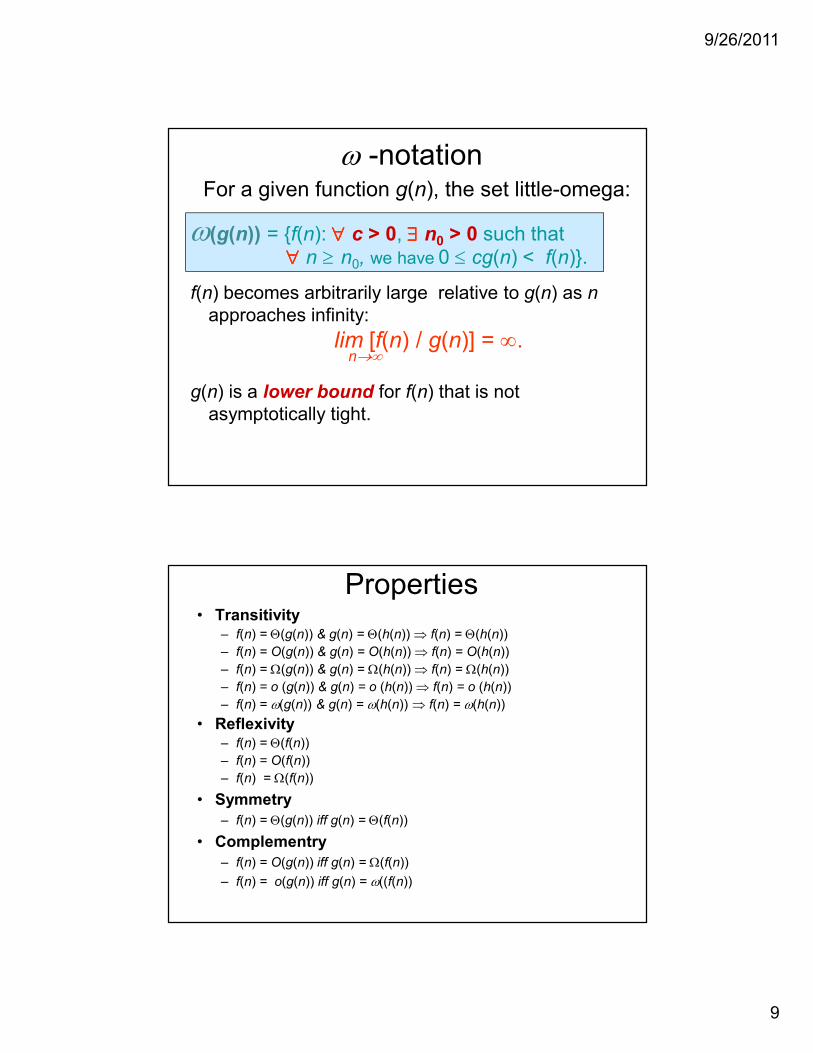
ω(g(n)) = f(n): ∀∀∀∀ c > 0, ∃∃∃∃ n0 > 0 such that ∀∀∀∀ n ≥ n0, we have 0 ≤ cg(n) < f(n).

ω -notation

f(n) becomes arbitrarily large relative to g(n) as n

approaches infinity:

lim [f(n) / g(n)] = ∞.n→∞

g(n) is a lower bound for f(n) that is not

asymptotically tight.

For a given function g(n), the set little-omega:

Properties• Transitivity

– f(n) = Θ(g(n)) & g(n) = Θ(h(n)) ⇒ f(n) = Θ(h(n))

– f(n) = O(g(n)) & g(n) = O(h(n)) ⇒ f(n) = O(h(n))

– f(n) = Ω(g(n)) & g(n) = Ω(h(n)) ⇒ f(n) = Ω(h(n))

– f(n) = o (g(n)) & g(n) = o (h(n)) ⇒ f(n) = o (h(n))

– f(n) = ω(g(n)) & g(n) = ω(h(n)) ⇒ f(n) = ω(h(n))

• Reflexivity– f(n) = Θ(f(n))

– f(n) = O(f(n))

– f(n) = Ω(f(n))

• Symmetry

– f(n) = Θ(g(n)) iff g(n) = Θ(f(n))

• Complementry

– f(n) = O(g(n)) iff g(n) = Ω(f(n))

– f(n) = o(g(n)) iff g(n) = ω((f(n))

9/26/2011

10

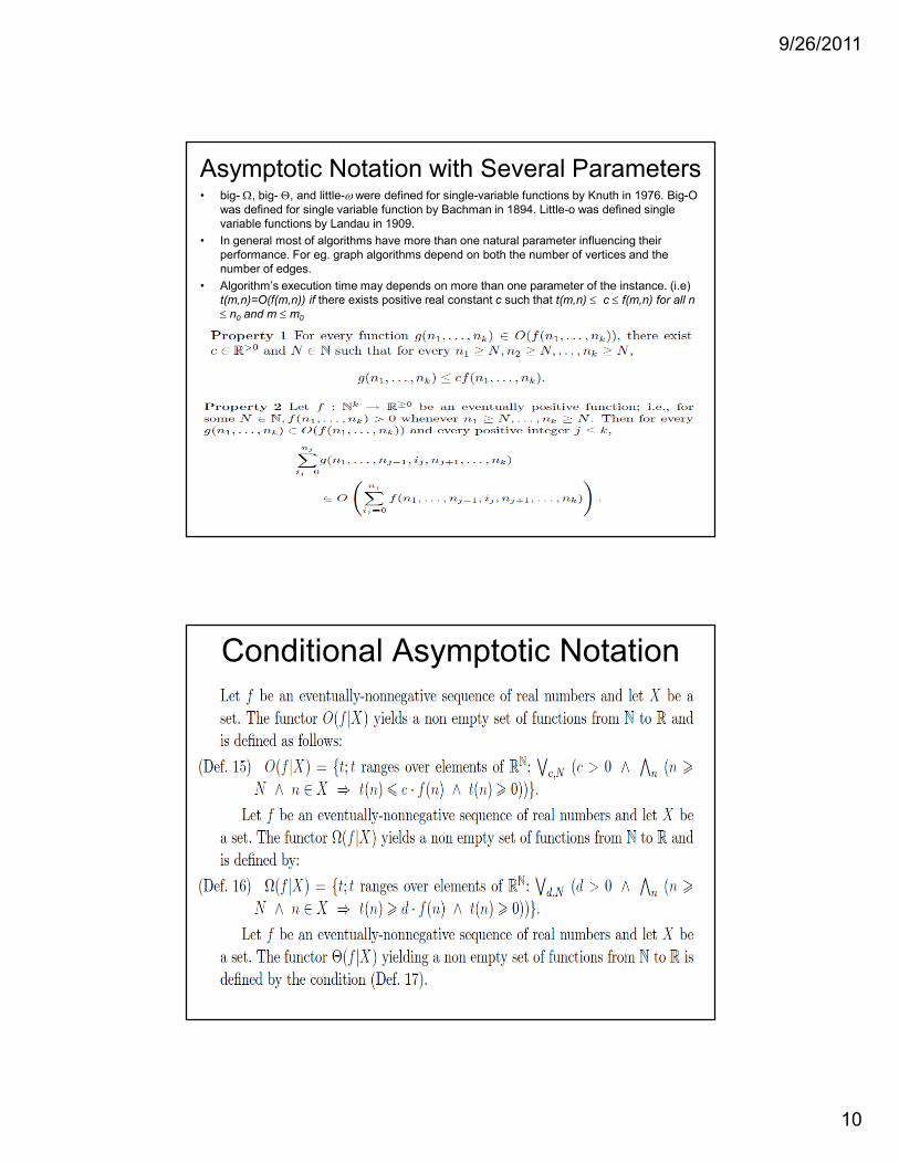
Asymptotic Notation with Several Parameters• big- Ω, big- Θ, and little-ω were defined for single-variable functions by Knuth in 1976. Big-O

was defined for single variable function by Bachman in 1894. Little-o was defined single

variable functions by Landau in 1909.

• In general most of algorithms have more than one natural parameter influencing their

performance. For eg. graph algorithms depend on both the number of vertices and the

number of edges.

• Algorithm’s execution time may depends on more than one parameter of the instance. (i.e)

t(m,n)=O(f(m,n)) if there exists positive real constant c such that t(m,n) ≤ c ≤ f(m,n) for all n

≤ n0 and m ≤ m0

Conditional Asymptotic Notation

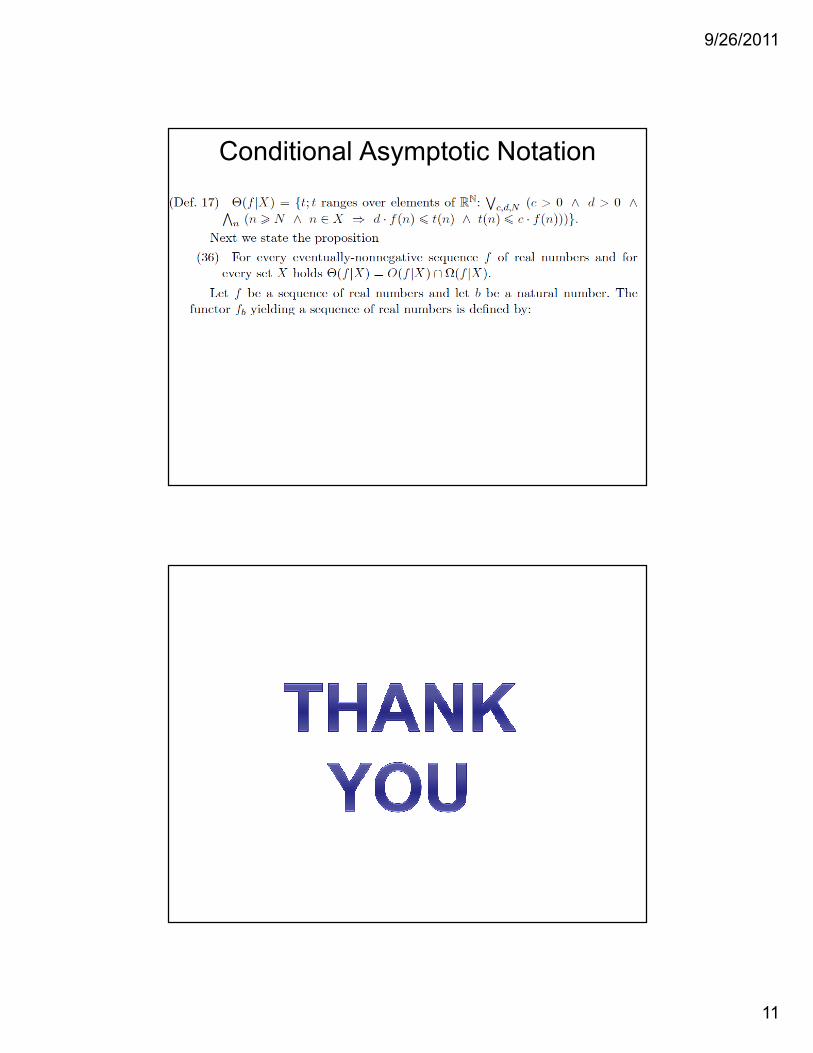
9/26/2011

11

Conditional Asymptotic Notation