Una nueva implementación para las ecuaciones de Navier-Stokes mediante KLE y elementos espectrales

Digital Object Identifier (DOI) 10.1007/s00211010383Numer. Math. (2002) 93: 201–221 Numerische
Mathematik
Convergence analysis and error estimatesfor a parallel algorithmfor solving the Navier-Stokes equations
I. Albarreal 1,, M.C. Calzada2,, J.L. Cruz2,, E. Fernandez-Cara1,,J. Galo2,, M. Mar ın2,
1 Department of Differential Equations and Numerical Analysis, University of Sevilla,Tarfia s/n, 41012 Sevilla, Spain; e-mail: [email protected]
2 Department of Computational Science and Numerical Analysis, University of Cordoba,Campus de Rabanales, Ed. C2-3, 14071 Cordoba, Spain; e-mail: [email protected]
Received April 20, 2001 / Revised version received May 21, 2001 /Published online March 8, 2002 –c© Springer-Verlag
Summary. This paper is concerned with the analysis of the convergenceand the derivation of error estimates for a parallel algorithmwhich is used tosolve the incompressibleNavier-Stokes equations. As usual, themain idea isto split the main differential operator; this allows to consider independentlythe two main difficulties, namely nonlinearity and incompressibility. Theresults justify the observed accuracy of related numerical results.
Mathematics Subject Classification (1991):65M12
1 Introduction
Let Ω ⊂ Rd be a regular bounded domain (d = 2 or 3) and assume that
T > 0. In this paper, we will consider a fluid governed by the Navier-Stokesequations inΩ × (0, T ), that is:
∂u
∂t− ν∆u+ (u · ∇)u+ ∇p = f in Ω × (0, T ),
∇ · u = 0 in Ω × (0, T ).(1)
Here,u = u(x, t) is the velocity field,p = p(x, t) is the pressure,ν > 0 isthe kinematic viscosity (a constant) andf = f(x, t) is the density function
Partially supported by D.G.E.S. (Spain), Proyecto PB98–1134 Partially supported by D.G.E.S. (Spain), Proyecto PB96–0986

202 I. Albarreal et al.
for a field of external forces. For simplicity, we have assumed in(1) thatthe fluid density is1. Of course,(1) has to be completed with appropriateboundary and initial conditions.
It is well known that the numerical solution of problems of this kindinvolves several major difficulties. Among them, let us emphasize the fol-lowing:
– The unknownsui are coupled through the incompressibility condition∇ · u = 0, which plays the role of an additional equation.
– The problem is nonlinear, owing to the presence of the term(u · ∇)u.
On the other hand, in many realistic situations,d = 3 andν is verysmall (once the variables have been adimensionalized,ν is the reciprocalof the Reynolds number and it may become of the order of10−5 or evensmaller). It is then usual to find flows with a very complicated structure,with high oscillations ofu andp in space and time. Accordingly, time andspace discretizations require many grid points in order to obtain an accuratedescription of the fluid.
All this has justified during the last decades an intensive research ofnumerical algorithms providing approximate solutions.
Usually, the numerical approximation procedure consists of two majorsteps. First, the equations are discretized in time and, then, the resulting(sub)problems are discretized in space.
There are many classical sequential schemes that can be used to dis-cretize in time, see [14]. Among those most frequently used, we find theso-calledfractional step methods, see [7]. The reason is that fractional stepdiscretization can lead to an effective splitting of the above mentioned maindifficulties. In this way, the task is reduced to the solution of a set of station-ary problems of two different kinds: (a)Quasilinear elliptic systemswherethe incompressibility condition has been ignored and (b)Linear systems ofthe Stokes kind.
In this paper, we are concerned with the convergence analysis and theobtention of error estimates for some fractional step algorithms which areparallel in time.
This paper is the sequel of [3] and [4]. It will be followed by [5], wherewe introduce also parallelization at the space approximation level. The al-gorithms and also the arguments discussed in the error estimates analysisare very close to those in [1].
Our motivation to consider parallel algorithms is two-fold. First, we no-tice that time parallelization enables to solve the resulting stationary prob-lems (quasilinear elliptic systems and Stokes-like systems) simultaneously.Secondly, we observe that parallelization in space simplifies notably the na-ture of the problems we have to solve. In particular, the techniques in [5]lead at the end to the solution of one-dimensional problems (see also [10]).
Convergence analysis and error estimates for a parallel algorithm 203
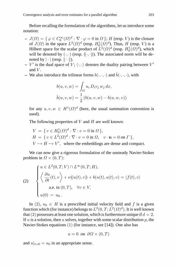
Before recalling the formulation of the algorithms, let us introduce somenotation:
– J(Ω) = ϕ ∈ C∞0 (Ω)d : ∇ · ϕ = 0 in Ω ; H (resp.V ) is the closure
of J(Ω) in the spaceL2(Ω)d (resp.H10 (Ω)d). Thus,H (resp.V ) is a
Hilbert space for the scalar product ofL2(Ω)d (resp.H10 (Ω)d), which
will be denoted by(·, ·) (resp.((·, ·))). The associated norm will be de-noted by| · | (resp.‖ · ‖).
– V ′ is the dual space ofV ; 〈·, ·〉 denotes the duality pairing betweenV ′andV .
– We also introduce the trilinear formsb(·, ·, ·) andb(·, ·, ·), with
b(u, v, w) =∫
Ωui Divj wj dx,
b(u, v, w) =12
(b(u, v, w) − b(u,w, v))
for any u, v, w ∈ H1(Ω)d (here, the usual summation convention isused).
The following properties ofV andH are well known:
V = v ∈ H10 (Ω)d : ∇ · v = 0 in Ω ,
H = v ∈ L2(Ω)d : ∇ · v = 0 in Ω, v · n = 0 onΓ ,V → H → V ′, where the embeddings are dense and compact.
We can now give a rigorous formulation of the unsteady Navier-Stokesproblem inΩ × (0, T ):
u ∈ L2(0, T ;V ) ∩ L∞(0, T ;H),⟨∂u
∂t(t), v
⟩+ ν((u(t), v)) + b(u(t), u(t), v) = 〈f(t), v〉
a.e. in(0, T ), ∀v ∈ V,
u(0) = u0 .
(2)
In (2), u0 ∈ H is a prescribed initial velocity field andf is a givenfunction which (for instance) belongs toL2(0, T ;L2(Ω)d). It is well knownthat(2)possesses at least one solution,which is furthermore unique ifd = 2.If u is a solution, thenu solves, together with some scalar distributionp, theNavier-Stokes equations(1) (for instance, see [14]). One also has
u = 0 on ∂Ω × (0, T )
andu|t=0 = u0 in an appropriate sense.

204 I. Albarreal et al.
An important property ofb(·, ·, ·) is thatb(u, v, v) = 0 for all u ∈ Vandv ∈ H1
0 (Ω)d. This is not true in general if∇ · u = 0. Since we areinterested in determining approximations ofu which are not necessarilydivergence-free, it is reasonable to replace the nonlinear term(u · ∇)u by
(u · ∇)u+12(∇ · u)u,
which is associated to the trilinear formb(u, u, v). Of course,
b(u, v, w) = b(u, v, w), ∀u ∈ V, ∀v, w ∈ H10 (Ω)d
and, also,b(u, v, v) = 0 for all v ∈ H10 (Ω)d (even when∇ · u = 0).
Obviously, the variational evolution equation in (2) can also be written interms ofb(·, ·, ·). This gives the following equivalent formulation:
u ∈ L2(0, T ;V ) ∩ L∞(0, T ;H),⟨∂u
∂t(t), v
⟩+ ν((u(t), v)) + b(u(t), u(t), v) = 〈f(t), v〉,
a.e. in(0, T ), ∀v ∈ V,
u(0) = u0 .
(3)
We are now going to specify the algorithms considered in this paper. Thenumerical approximation is carried out at two levels:
a)Approximation with respect to the time variablet – First, the time deriva-tives are replaced by difference quotients. Accordingly, one is led to theformulation of stationary subproblems of two kinds where only one of theabove mentioned difficulties is conserved. At each time step, two of thesesubproblems can be solved simultaneously. Their solutions can then be usedto compute an approximation at the next value oft.
b)Approximation with respect to the space variablesxi – This is needed tosolve the previous subproblems. Among other possibilities, we will use, asin [3] and [4], finite element methods, although the theoretical argumentsalso hold for other approximations.
First level: Assume that[0, T ] is divided inN subintervals of lengthτ(τ = T/N ) and assume that three parametersσ, θ, µ ∈ (0, 1) are given.First, we set
u0 = u0 .(4)
Convergence analysis and error estimates for a parallel algorithm 205
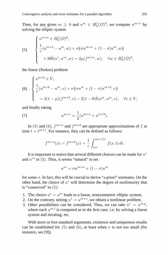
Then, for any givenm ≥ 0 andum ∈ H10 (Ω)d, we computeum+1 by
solving the elliptic system
um+a ∈ H10 (Ω)d,
1τ(um+a − um, w) + ν((σum+a + (1 − σ)um, w))
+ 2θb(u∗, u∗∗, w) = 2µ(fm+a, w), ∀w ∈ H10 (Ω)d,
(5)
the linear (Stokes) problem
um+b ∈ V,
1τ(um+b − um, v) + ν((σum + (1 − σ)um+b, v))
= 2(1 − µ)(fm+b, v) − 2(1 − θ)b(um, um, v), ∀v ∈ V,
(6)
and finally taking
um+1 =12(um+a + um+b).(7)
In (5) and(6), fm+a andfm+b are appropriate approximations off attime t = tm+1. For instance, they can be defined as follows:
fm+a(x) = fm+b(x) =1τ
∫ (m+1)τ
mτf(x, t) dt.
It is important to notice that several different choices can be made foru∗andu∗∗ in (5). Thus, it seems “natural” to set
u∗∗ = σum+a + (1 − σ)um
for someσ. In fact, this will be crucial to derive “a priori” estimates. On theother hand, the choice ofu∗ will determine the degree of nonlinearity thatis “conserved” in(5):
1. The choiceu∗ = um leads to a linear, nonsymmetric elliptic system.2. On the contrary, settingu∗ = um+a, we obtain a nonlinear problem.3. Other possibilities can be considered. Thus, we can takeu∗ = um,p,
where eachum,i is computed as in the first case, i.e. by solving a linearsystem and iterating, etc.
With more or less standard arguments, existence and uniqueness resultscan be established for(5) and (6), at least whenν is not too small (forinstance, see [9]).

206 I. Albarreal et al.
Second level:For simplicity, wewill only present the completely discretizedproblems (in time and space) whenΩ is a polyhedral domain and a standardP -Lagrange finite element approximation is used (# ≥ 2).
Thus, letTh be a uniformly regular family of triangulations ofΩ (inthe sense of [2]) and letWh be the corresponding (finite dimensional) sub-space ofH1
0 (Ω)d formed by all functionsvh ∈ C0(Ω)d whose componentscoincide with a polynomial of degree≥ # on eachK ∈ Th and vanish on∂Ω.
We will also introduce the spacesVh, with
Vh =vh ∈ Wh :
∫K
(∇ · vh) dx = 0, ∀K ∈ Th
.(8)
We will discretize(4)–(7) as follows: First,u0h is the orthogonal projection
of u0 in the spaceWh (for theL2-scalar product), i.e.
(u0h, vh) = (u0, vh), ∀vh ∈ Wh, u0
h ∈ Wh .(9)
Then, for any givenm ≥ 0 andumh ∈ Wh, we computeu
m+1h by solving
um+ah ∈ Wh,
1τ(um+a
h − umh , wh) + ν((σum+a
h + (1 − σ)umh , wh))
+ 2θbh(u∗h, u
∗∗h , wh) = 2µ(fm+a, wh), ∀wh ∈ Wh ,
(10)
and the linear problem
um+bh ∈ Vh,
1τ(um+b
h − umh , vh) + ν((σum
h + (1 − σ)um+bh , vh))
= 2(1 − µ)(fm+b, vh) − 2(1 − θ)b(umh , u
mh , vh), ∀vh ∈ Vh ,
(11)
and by taking
um+1h =
12(um+a
h + um+bh ).(12)
Of course, we have in mind to chooseu∗h andu
∗∗h as before: we will take
u∗∗h = σum+a
h + (1 − σ)umh
and (for instance)u∗h = um
h , u∗h = um+a
h , etc.The numerical behavior of scheme(9)–(12) has been illustrated in [3]
and [4] through the solution of several test problems. In fact, the choice ofVh we have made in(8) is not optimal forP -Lagrange finite elements with# ≥ 3 but, for simplicity, this will be the one considered here.

Convergence analysis and error estimates for a parallel algorithm 207
The rest of this paper is organized as follows. In Sect. 2, we recall aconvergence result for the totally discretized algorithm(9)–(12) that is es-sentially contained in [4]. For completeness, we also recall the main ideasused in the proof. In Sect. 3, we derivee some error estimates in a particularcase. In this context, wewill only consider the semi-discretized scheme. Thederivation of error estimates for scheme(9)–(12) is more intrincate and willbe the goal of a forthcoming paper.
2 A convergence result
In the sequel,C denotes a generic positive constant only depending on thedataΩ, T , ν, u0 andf and, possibly, the parametersσ, θ andµ.
In the finite dimensional spaceWh , ‖ · ‖ and| · | are equivalent norms.More precisely, we have
λ|wh| ≤ ‖wh‖ ≤ S(h)|wh|, ∀wh ∈ Wh(13)
for someoptimalquantitiesλ andS(h). It is known thatλ = λ1/21 ,λ1 being
the first eigenvalue of the Laplace operator inΩ with Dirichlet boundaryconditions. On the other hand, in view of the uniform regularity ofTh,S(h) can be estimated in the form
S(h) ≤ C
h(14)
(see [14]). This will be crucial in the proof of the convergence of the scheme(we are thus forced to consider uniformly regular familiesTh).
We also have
|b(vh, vh, wh)| ≤ S(h)|vh|2‖wh‖, ∀vh, wh ∈ Wh(15)
for someoptimal S(h). Of course,S(h) ≤ C S(h)2, but much better esti-mates hold because of the particular choice ofWh we have made. Specifi-cally, for all ε > 0, we have
S(h) ≤ Cε
h1+εif d = 2;(16)
on the other hand,
S(h) ≤ C
h3/2 if d = 3(17)
(see [14] for more details).

208 I. Albarreal et al.
For each time stepτ and eachh > 0, let us introduce the functionsuτh ,vτh , wτh , zτh , uτh , vτh andwτh , which are given as follows:uτh, vτh, wτh, zτh : [0, T ] → Wh are piecewise constant, with
uτh(t) = umh , vτh(t) = um+a
h , wτh(t) = um+bh
and zτh(t) = σum+ah + (1 − σ)um
h in [mτ, (m+ 1)τ ),uτh, vτh, wτh : [0, T ] → Wh are continuous and piecewise linear, with
uτh(mτ) = umh , vτh(mτ) = um+a
h , wτh(mτ) = um+bh .
Theorem 1 Assume thatσ ∈ (12 , 1], u∗∗
h = σum+ah + (1 − σ)um+b
h and,for instance,u∗
h = umh in (10). There exist constantsK0 andK1 , only
depending onΩ, |u0|, ‖f‖L2(0,T ;H) , ν andσ, such that, whenever
τS(h)2 ≤ K0, τ S(h)2 ≤ K1,(18)
we have:
1. There exist subsequencesuτ ′h′ , . . . , wτ ′h′ that converge strongly in thespaceL2(0, T ;L2(Ω)d), weakly inL2(0, T ;H1
0 (Ω)d) and also weakly-∗in L∞(0, T ;L2(Ω)d) to the same functionu.
2. The limit of any such subsequence is a solution of(2).3. Consequently, whend = 2, the whole sequencesuτh , . . . , wτh converge
(in the above sense) to the unique solution of(2).4. Finally, if d = 2 andτ andh satisfy
τS(h)2 → 0, τ S(h)2 → 0,(19)
we also have strong convergence of the whole sequences in the spaceL2(0, T ;H1
0 (Ω)d). Remark 1Obviously,(18)canbeviewedasastability condition. Inpractice,it means thatτ cannot be too large whenh is small: it must be of the order ofh2 (resp.h3) if d = 2 (resp.d = 3). Accordingly, Theorem 1 says (amongother things) that scheme(4)–(7) is conditionally stable. Remark 2The argument used in the proof of Part 4 shows that the strongconvergence remains true whend = 3 (at least for a subsequence) providedconditions(19) are fulfilled and the solutionu satisfies the energy identityat timet = T , (see(28)).
The proof of Theorem 1is essentially given in [4]. Other similar results forrelated but different algorithms are given in [6] and [8]. For completeness,let us give a sketch of it. The proof consists of several steps:

Convergence analysis and error estimates for a parallel algorithm 209
First step. Some “a priori” estimates
For simplicity, we droph in this step and in the following one. Let us takew = σum+a + (1 − σ)um in (10) andv = um+b in (11). Then, usingthe fact that12 < σ ≤ 1, we find after some computations the followingfundamental estimates
max0≤m≤N
|um|2 +N∑
m=0
|um+a − um|2 +N∑
m=0
|um+b − um|2
+τN∑
m=0
‖um‖2 + τ
N∑m=0
‖um+b‖2 + τ
N∑m=0
‖um+a − um‖2 ≤ C,(20)
whereC depends only ofΩ, T, ν, |u0|, ‖f‖L2(Q) andσ.From(20), it is not difficult to derive uniform estimates for all the func-
tionsuτ , vτ , etc. Namely, we find that
‖uτ‖L∞(0,T ;L2(Ω)d) + ‖uτ‖L2(0,T ;H10 (Ω)d) ≤ C
and the same holds forvτ , wτ , uτ , vτ andwτ .(21)
It is also easy to see that
‖uτ − vτ‖L2(0,T ;L2(Ω)d) ≤ C√τ
and the same holds foruτ − wτ , uτ − uτ , etc.(22)
Second step. Compactness inL2(0, T ;L2(Ω)d)
Let us extend by zero the functionsuτ outside[0, T ]. Let us denote againby uτ these extensions. Then, it can be proved that, for anyβ ∈ (0, 1
4), theFourier transformuτ of uτ satisfies the estimates
∫ +∞
−∞|s|2β|uτ (s)|2 ds ≤ Cβ .(23)
This, togetherwith the uniformbound inL2(0, T ;L2(Ω)d), yields compact-ness in this last space. Indeed,(23) implies thatuτ is uniformly boundedin the Sobolev spaceHβ(0, T ;L2(Ω)d) for eachβ ∈ (0, 1
4) and it is wellknown thatHβ(0, T ;L2(Ω)d) is compactly embedded inL2(0, T ;L2(Ω)d).

210 I. Albarreal et al.
Third step. The converging subsequences
From the estimates in the first step, we see that it is possible to extract asubsequenceuτ ′h′ satisfying
uτ ′h′ → u weakly inL2(0, T ;H10 (Ω)d)
and weakly-∗ in L∞(0, T ;L2(Ω)d)
ash′ → 0, τ ′ → 0. On the other hand, in accordance with the second step,we also have
uτ ′h′ → u strongly inL2(Q)d.(24)
Recalling(22), we see that similar convergence properties must hold forvτ ′h′ , . . . , wτ ′h′ .
In particular, this implies thatu ∈ L2(0, T ;V ) ∩ L∞(0, T ;H).
Fourth step. Any limit pointu solves(2)
Assume thatϕ ∈ J(Ω)and letψ bea function inC1([0, T ]), withψ(T ) = 0.It is not difficult to find a sequenceϕh , with ϕh ∈ Vh for all h, such thatϕh → ϕ strongly inH1
0 (Ω)d. Then we have
−∫ T
0(uτh(t), ψ′(t)ϕh) dt
+ν
2
∫ T
0(( uτh(t) + σvτh(t) + (1 − σ)wτh(t), ψ(t)ϕh )) dt
+θ∫ T
0b(uτh(t), σvτh(t) + (1 − σ)uτh(t), ψ(t)ϕh)dt
+(1 − θ)∫ T
0b(uτh(t), uτh(t), ψ(t)ϕh) dt
= (uτh(0), ϕh)ψ(0) +∫ T
0(µf1τ (t) + (1 − µ)f2τ (t), ψ(t)ϕh) dt,
where the functionsf1τ andf2τ converge strongly tof inL2(0, T ;L2(Ω)d).In view of this identity and the convergence results we have proved in theprevious steps, it is possible to deduce the following for any limit pointu:
−∫ T
0(u(t), ψ′(t)ϕ) dt+ ν
∫ T
0((u(t), ψ(t)ϕ)) dt
+∫ T
0b(u(t), u(t), ψ(t)ϕ) dt
= (u0, ϕ)ψ(0) +∫ T
0(f(t), ψ(t)ϕ) dt.
(25)

Convergence analysis and error estimates for a parallel algorithm 211
By density,(25) must also hold for anyϕ ∈ V . This proves thatu solvesthe evolution equation in(3). Finally, by imposingψ(0) = 1, we find that
(u0, ϕ) = −∫ T
0(u(t), ψ′(t)ϕ) dt+ ν
∫ T
0((u(t), ψ(t)ϕ)) dt
+∫ T
0b(u(t), u(t), ψ(t)ϕ) dt−
∫ T
0(f(t), ψ(t)ϕ) dt
= (u(0), ϕ)
for anyϕ ∈ V , whence the initial condition in(2) is also satisfied. Thisproves thatu is a solution of(2).
Fifth step. Strong convergence
Assume thatd = 2 andτ andh are chosen in such a way thatτS(h)2 → 0andτ S(h)2 → 0. The strong convergence ofuτh in L2(0, T ;H1
0 (Ω)d) canbe proved as follows:
First, we notice that a sequenceu+h can be found, withu+
h ∈ L2(0,T ;Wh) for all h, such that
u+h → u strongly inL2(0, T ;H1
0 (Ω)d).(26)
Then, we introduce the following quantityXτh (whereατh → 0):
Xτh = 2|uNh − u(T )|2 +
N−1∑m=0
12|um+a
h − um+bh |2
+(2σ − 1)|um+ah − um
h |2 + |um+bh − um
h |2
+2ν∫ T
0‖zτh(t) − u+
h (t)V ert2 dt
+2ν∫ T
0‖wτh(t) − u+
h (t)‖2 dt+ 2νN−1∑m=0
((umh − um+b
h , um+bh ))
+2
T∫0
b(uτh(t), uτh(t), wτh(t)) dt+ ατh
∫ T
0‖uτh(t)‖2
h dt
+ατh
∫ T
0‖wτh(t)‖2 dt
(recall thatzτh = σvτh + (1 − σ)uτh).Assuming thatuN
h′ converges weakly inL2(Ω)d to χ ash′ → 0 andτ ′ → 0, we can subsequently show:

212 I. Albarreal et al.
– That the following relation holds:
(χ− u(T ), v) = 0, ∀v ∈ H.(27)
Here, we use the fact thatu satisfies the energy identity at timet = T ,that is
12|u(T )|2 + ν
∫ T
0‖u(t)‖2 dt =
12|u0|2 +
∫ T
0(f(t), u(t)) dt.(28)
– Also, thatXτ ′h′ → 0 ash′ → 0 andτ ′ → 0.(29)
– Finally, that
Xτh ≥∫ T
0‖zτ ′h′(t) − u+
h′(t)‖2 dt ≥ 0.(30)
From(29) and(30), we obtain in particular that∫ T
0‖zτ ′h′(t) − u+
h′(t)‖2 dt → 0,
whence it is clear thatuτ ′h′ converges strongly. This concludes the proof ofthe theorem.
3 Error estimates
As in [12] and [13], we will use the following definition to determine theorder of accuracy of a scheme:
Definition 1 Let X be a Banach space for the norm‖ · ‖X and letF :[0, T ] → X be a continuous function. Lett(τ)
m Nm=0 be given, withτ =
T/N and
0 = t(τ)0 < . . . < t(τ)
m < t(τ)m+1 < . . . < t
(τ)N = T,
max0≤m≤N−1
|t(τ)m+1 − t(τ)
m | ≤ δτ → 0.
Assume that, for eachτ , a piecewise constant functionFτ : [0, T ] → X is
given, withFτ (t) = Fτ (t(τ)m ) in [mτ, (m+ 1)τ). It will be said thatFτ is a
weak approximation ofF in X of orderα if one has
τ
N∑m=0
‖F (t(τ)m ) − Fτ (t(τ)
m )‖2X ≤ Cτ2α
for someC independent ofτ . On the other hand, it will be said thatFτ is astrong approximation ofF in X of orderα if
max0≤m≤N
‖F (t(τ)m ) − Fτ (t(τ)
m )‖2X ≤ Cτ2α.

Convergence analysis and error estimates for a parallel algorithm 213
In the sequel, the following discrete Gronwall lemma will be used (for aproof, see [11], p. 369):
Lemma 1 Assume thatk, B andam , bm , cm , γm are given nonnegativenumbers such that
an + k
n∑m=0
bm ≤ k
n∑m=0
γmam + k
n∑m=0
cm +B, ∀n ≥ 0.(31)
Assume thatkγm < 1 for all m and setσm ≡ (1 − kγm)−1. Then
an + k
n∑m=0
bm ≤ exp
(k
n∑m=0
σmγm
)k
n∑m=0
cm +B
,
∀n ≥ 0.(32) Remark 3If γn = 0 in the first sum in the right of(31), then (32) issatisfied for allk > 0, with all σm ≡ 1. In this case, if the coefficientsγm
are uniformly bounded andn ≤ [T/k], we also have:
an + k
n∑m=0
bm ≤ Ck
n∑m=0
cm + CB, ∀n ≥ 0.(33)
We will now deduce error estimates for the semi-discretized (in time)
schemes. We will have to assume that:
– The dataf andu0 are regular enough, more precisely
u0 ∈ H2(Ω)d ∩ V , f,∂f
∂t∈ L∞(0, T ;L2(Ω)d).(34)
– There exists a strong regular solution of(1) defined in the whole interval[0, T ] (if d = 3). More precisely, we will assume that
supt∈[0,T ]
‖u(t)‖ < +∞.(35)
Under hypotheses(34) and(35), it is proved in [11] that
supt∈[0,T ]
‖u(t)‖H2 + |ut(t)| + |∇p(t)| ≤ Cu ,(36)
∫ T
0‖ut(t)‖2 dt ≤ Cu(37)
and ∫ T
0t‖utt(t)‖2
H−1 dt ≤ Cu .(38)
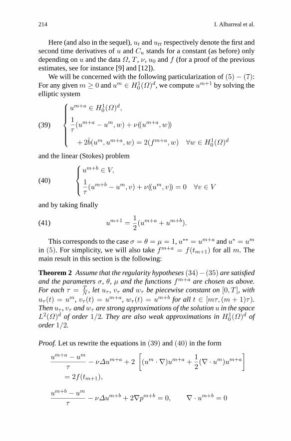
214 I. Albarreal et al.
Here (and also in the sequel),ut andutt respectively denote the first andsecond time derivatives ofu andCu stands for a constant (as before) onlydepending onu and the dataΩ, T , ν, u0 andf (for a proof of the previousestimates, see for instance [9] and [12]).
We will be concerned with the following particularization of(5) − (7):For any givenm ≥ 0 andum ∈ H1
0 (Ω)d, we computeum+1 by solving theelliptic system
um+a ∈ H10 (Ω)d,
1τ(um+a − um, w) + ν((um+a, w))
+ 2b(um, um+a, w) = 2(fm+a, w) ∀w ∈ H10 (Ω)d
(39)
and the linear (Stokes) problemum+b ∈ V,
1τ(um+b − um, v) + ν((um, v)) = 0 ∀v ∈ V
(40)
and by taking finally
um+1 =12(um+a + um+b).(41)
This corresponds to the caseσ = θ = µ = 1,u∗∗ = um+a andu∗ = um
in (5). For simplicity, we will also takefm+a = f(tm+1) for all m. Themain result in this section is the following:
Theorem 2 Assume that the regularity hypotheses(34)− (35) are satisfiedand the parametersσ, θ, µ and the functionsfm+a are chosen as above.For eachτ = T
N , let uτ , vτ andwτ be piecewise constant on[0, T ], withuτ (t) = um, vτ (t) = um+a, wτ (t) = um+b for all t ∈ [mτ, (m + 1)τ).Thenuτ , vτ andwτ are strong approximations of the solutionu in the spaceL2(Ω)d of order 1/2. They are also weak approximations inH1
0 (Ω)d oforder1/2.
Proof.Let us rewrite the equations in(39) and(40) in the form
um+a − um
τ− ν∆um+a + 2
[(um · ∇)um+a +
12(∇ · um)um+a
]= 2f(tm+1),
um+b − um
τ− ν∆um+b + 2∇pm+b = 0, ∇ · um+b = 0
Convergence analysis and error estimates for a parallel algorithm 215
and let us introduce the following velocity errors at timetm+1:
em+a = u(tm+1) − um+a, em+b = u(tm+1) − um+b
andem+1 = u(tm+1) − um+1.
We are going to derive appropriate estimates forem, em+a andem+b.They will show that the piecewise constant functionsuτ , vτ andwτ re-spectively associated toum, um+a andum+b are strong approximations inL2(Ω)d of order1/2 and also weak approximations inH1
0 (Ω)d of order1/2.
Let us introduce the truncation errorRm , which is given as follows:
u(tm+1) − u(tm)τ
− ν∆u(tm+1) + (u(tm+1) · ∇)u(tm+1)
+∇p(tm+1) = f(tm+1) +Rm,(42)
Obviously, we have
Rm =u(tm+1) − u(tm)
τ− ut(tm+1)
=1τ
∫ tm+1
tm
(t− tm)utt(t) dt.(43)
From(42) and the equation satisfied byum+a, one has
1τ(em+a − em) − ν∆em+a
= 2[(um · ∇)um+a +
12(∇ · um)um+a
]−(u(tm+1) · ∇)u(tm+1) − ∇p(tm+1) − f(tm+1) +Rm .
(44)
Let us compute the scalar product of(44) by 2τem+a and let us use theidentity
(a− b, 2a) = |a|2 − |b|2 + |a− b|2.(45)
Then we find
|em+a|2 − |em|2 + |em+a − em|2 + 2τν‖em+a‖2
= 4τ b(um, um+a, em+a) − 2τ b(u(tm+1), u(tm+1), em+a)
− 2τ(∇p(tm+1), em+a) − 2τ(f(tm+1), em+a)
+ 2τ(Rm, em+a).
(46)

216 I. Albarreal et al.
On the other hand, from(42) and the equation satisfied byum+b, we alsosee that
1τ(em+b − em) − ν∆em+b = −(u(tm+1) · ∇)u(tm+1)
+ 2∇pm+b − ∇p(tm+1) + f(tm+1) +Rm.
(47)
Now, let us compute the scalar product of(47) by 2τem+b and let us applyagain(45). We obtain:
|em+b|2 − |em|2 + |em+b − em|2 + 2τν‖em+b‖2
= −2τ b(u(tm+1), u(tm+1), em+b)
+ 4τ(∇pm+b, em+b) − 2τ(∇p(tm+1), em+b)
+ 2τ(f(tm+1), em+b) + 2τ(Rm, em+b).
(48)
Notice that, in(48), the pressure terms vanish, since∇·em+b = 0. From(46) and(48), we obtain the following identity:
12
(|em+a|2 + |em+b|2
)− |em|2 +
12|em+a − em|2
+12|em+b − em|2 + τν‖em+a‖2 + τν‖em+b‖2
= 2τ b(um, um+a, em+a) − τ b(u(tm+1), u(tm+1), em+a)
− τ b(u(tm+1), u(tm+1), em+b)
− τ(∇p(tm+1), em+a − em+b) + τ(f(tm+1), em+b − em+a)
+ τ(Rm, em+a) + τ(Rm, em+b).
(49)
After some manipulation, we can rewrite the first three terms in the righthand side as follows:
2τ b(um, um+a, em+a) − τ b(u(tm+1), u(tm+1), em+a)
− τ b(u(tm+1), u(tm+1), em+b)
= 2τ b(em, em+a, u(tm+1)) − 2τ b(u(tm) − u(tm+1), em+a, u(tm+1))
+ τ b(u(tm+1), u(tm+1), em+a − em)
+ τ b(u(tm+1), u(tm+1), em − em+b).

Convergence analysis and error estimates for a parallel algorithm 217
Accordingly,(49) can be put into the form
12
(|em+a|2 + |em+b|2
)− |em|2 +
12|em+a − em|2
+12|em+b − em|2 + τν‖em+a‖2 + τν‖em+b‖2
= 2τ b(em, em+a, u(tm+1))
− 2τ b(u(tm) − u(tm+1), em+a, u(tm+1))
+ τ b(u(tm+1), u(tm+1), em+a − em)
+ τ b(u(tm+1), u(tm+1), em − em+b)
− τ(∇p(tm+1), em+a − em+b) + τ(f(tm+1), em+b − em+a)
+ τ(Rm, em+a) + τ(Rm, em+b)
(50)
Let us now estimate the terms in the right hand side of(50). First,∣∣∣τ(Rm, em+a) + τ(Rm, em+b)∣∣∣ ≤ τ‖Rm‖H−1(‖em+a‖ + ‖em+b‖)
≤ 2τν
‖Rm‖2H−1 +
τν
4‖em+a‖2 +
τν
4‖em+b‖2.(51)
Thus, taking(43) into account, one has:
∣∣τ(Rm, em+a) + τ(Rm, em+b)∣∣
≤ τ
(∫ tm+1
tm
t‖utt(t)‖2H−1 dt
)
+τν
4‖em+a‖2 +
τν
4‖em+b‖2.
(52)
Secondly,
|τ(f(tm+1), em+b − em+a)|= |τ(f(tm+1), em − em+a) + τ(f(tm+1), em+b − em)|
≤ 6τ2|f(tm+1)|2 +112
|em+a − em|2 +112
|em+b − em|2.(53)
We also have
|τ(∇p(tm+1), em+a − em+b)|= |τ(∇p(tm+1), em+a − em) + τ(∇p(tm+1), em − em+b)|
≤ 6τ2|∇p(tm+1)|2 +112
|em+a − em|2 +112
|em+b − em|2.(54)

218 I. Albarreal et al.
On the other hand, it is not difficult to check that∣∣∣2τ b(em, em+a, u(tm+1)) − 2τ b(u(tm) − u(tm+1), em+a, u(tm+1))∣∣∣
≤ Cτ |em| · ‖em+a‖ · ‖u(tm+1)‖H2
+Cτ |u(tm) − u(tm+1)| · ‖em+a‖ · ‖u(tm+1)‖H2
≤ Cuτ |em|2 + Cuτ |u(tm) − u(tm+1)|2 +τν
4‖em+a‖2
≤ Cuτ |em|2 + Cuτ2∫ tm+1
tm
|ut(t)|2 dt+τν
4‖em+a‖2.(55)
Finally, we have∣∣∣τ b(u(tm+1), u(tm+1), em+a − em)
+τ b(u(tm+1), u(tm+1), em+b − em)∣∣∣
≤ Cτ‖u(tm+1)‖ · ‖u(tm+1)‖H2 · |em+a − em|+Cτ‖u(tm+1)‖ · ‖u(tm+1)‖H2 · |em+b − em|≤ Cuτ
2‖u(tm+1)‖2 +112
|em+a − em|2 +112
|em+b − em|2.(56)
Taking into account that
|em+1|2 ≤ 12
[|em+a|2 + |em+b|2
]and combining the estimates(52) − (56) and(50), we obtain:
|em+1|2 − |em|2 +12|em+a − em|2 +
12|em+b − em|2
+τν‖em+a‖2 + τν‖em+b‖2
≤ τ
∫ tm+1
tm
t‖utt(t)‖2H−1 dt+ Cuτ
2∫ tm+1
tm
|ut(t)|2 dt
+Cuτ2‖u(tm+1)‖2 + 6τ2|f(tm+1)|2 + 6τ2|∇p(tm+1)|2
+Cuτ |em|2 +τν
2‖em+a‖2 +
τν
4‖em+b‖2
+14|em+a − em|2 +
14|em+b − em|2.(57)
Consequently,
|em+1|2 − |em|2 +14|em+a − em|2 +
14|em+b − em|2
Convergence analysis and error estimates for a parallel algorithm 219
+τν
2‖em+a‖2 +
3τν4
‖em+b‖2
≤ Cuτ |em|2 + τ
∫ tm+1
tm
t‖utt(t)‖2H−1 dt
+τ2
[Cu
∫ tm+1
tm
|ut(t)|2dt+ Cu‖u(tm+1)‖2
+6|f(tm+1)|2 + 6|∇p(tm+1)|2].(58)
The addition of these inequalities form = 0, . . . , n and the fact that|e0| = 0yield the following estimates:
|en+1|2 +n∑
m=0
|em+a − em|2 + |em+b − em|2
+τνn∑
m=0
‖em+a‖2 + ‖em+b‖2
≤ Cuτ
n∑m=0
|em|2 + Cuτ2
n∑m=0
‖u(tm+1)‖2
+Cτ2n∑
m=0
|f(tm+1)|2 + Cτ2n∑
m=0
|∇p(tm+1)|2 + Cuτ.(59)
We will now estimate the last three terms in the right-hand side of(59).To this end, we will use(35), (36) and(37). We have:
τ
n∑m=0
|f(tm+1)|2 ≤ τ
N−1∑m=0
supt∈[0,T ]
|f(t)|2
≤ T supt∈[0,T ]
|f(t)|2 = C .(60)
Similarly,
τ
n∑m=0
|∇p(tm+1)|2 ≤ Cu(61)
and
τ
n∑m=0
‖u(tm+1)‖2 ≤ Cu .(62)

220 I. Albarreal et al.
Accordingly, we are led to the following:
|en+1|2 +n∑
m=0
|em+a − em|2 + |em+b − em|2
+ τν
n∑m=0
‖em+a‖2 + ‖em+b‖2
≤ Cuτ
n∑m=0
|em|2 + Cuτ.
(63)
In particular
|en+1|2 ≤ Cuτ
n∑m=0
|em|2 + Cuτ(64)
for all n. Let us now apply Lemma 1 to(64). This leads to the estimates
|en+1|2 ≤ Cuτ ∀n = 0, 1, . . . , N − 1(65)
andn∑
m=0
|em|2 ≤N−1∑m=0
|em|2 ≤ Cu .(66)
Combining(63) and(66), we also obtain that
|en+1|2 +n∑
m=0
|em+a − em|2 + |em+b − em|2
+τνn∑
m=0
‖em+a‖2 + ‖em+b‖2
≤ Cuτ
(67)
We also have
|em+b|2 ≤ 2|em+b − em|2 + 2|em|2 ≤ Cuτ,(68)
and
|em+a|2 ≤ 2|em+a − em|2 + 2|em|2 ≤ Cuτ.(69)
Consequently, ifuτ , vτ andwτ are defined as before, we have that
max0≤m≤N
|u(tm) − uτ (tm)|2 = max0≤m≤N
|em|2 ≤ Cuτ
and similar properties hold forvτ andwτ . This shows thatuτ , vτ andwτ
are strong approximations ofu in the spaceL2(Ω)d of order1/2.On the other hand, we see from(67) that
τ
n∑m=0
‖u(tm) − uτ (tm)‖2 ≤ Cuτ
and (again) the same holds forvτ andwτ . Accordingly,uτ , vτ andwτ areweak approximations ofu in the spaceH1
0 (Ω)d of order1/2. This completesthe proof.
Convergence analysis and error estimates for a parallel algorithm 221
References
1. J. Blasco: Thesis, Universitat Politecnica de Catalunya, Barcelona 19962. P.G. Ciarlet: The Finite Element Method for Elliptic Problems, North-Holland, Ams-
terdam 19793. J.L. Cruz et al.: A parallel algorithm for solving the incompressible Navier-Stokes
problem. Comput. Math. Appl.25(No. 9), 51–58 (1993)4. J.L. Cruz et al.: A convergence result for a parallel algorithm for solving the Navier-
Stokes equations. Comput. Math. Appl.35(4), 71–88 (1998)5. J.L. Cruz et al.: Time and space parallelization of the Navier-Stokes equations, in
preparation6. E. Fernandez-Cara, M. Marın: The convergence of two numerical schemes for the
Navier-Stokes equations. Numer. Math.55, 33–60 (1989)7. R. Glowinski: Numerical Methods for Nonlinear Variational Problems, 2nd Ed.
Springer-Verlag, New York 19848. P.Kloucek, F.S.Rys.: Stability of the fractional stepθ-scheme for nonstationaryNavier-
Stokes equations. SIAM J. Numer. Anal.31(5), 1312–1335 (1994)9. J.L. Lions:Quelques Methodesde ResolutiondesProblemesauxLimitesnonLineaires,
Dunod, Gauthiers-Villars, Paris 196910. T. Liu et al.: A parallel splitting-up method for partial differential equations and its
applications to Navier-Stokes equations, Math. Models and Numer. Anal.26(6), 673–708
11. J.G. Heywood, R. Rannacher: Finite element approximation of the nonstationaryNavier-Stokesproblem, I. Regularity of solutionsand second-order estimates for spatialdiscretization. SIAM J. Numer. Anal.19(2), 275–311 (1982)
12. J. Shen: On error estimates of projection methods for Navier-Stokes equations: first-order schemes. SIAM J. Numer. Anal.29(1), 57–77 (1992)
13. J. Shen: Remarks on the pressure error estimates for the projection methods. Numer.Math.67, 513–520 (1994)
14. R. Temam : Navier-Stokes Equations, 2nd Ed. North-Holland, Amsterdam 1977
Copyright © 2022 FDOKUMEN