symmetryS S

Article

Exact Solutions to the Navier–Stokes Equationswith Couple Stresses

Evgenii S. Baranovskii 1,* , Natalya V. Burmasheva 2,3 , Evgenii Yu. Prosviryakov 2,4

�����������������

Citation: Baranovskii, E.S.;

Burmasheva, N.V.; Prosviryakov, E.Y.

Exact Solutions to the Navier–Stokes

Equations with Couple Stresses.

Symmetry 2021, 13, 1355. https://

doi.org/10.3390/sym13081355

Academic Editor: Constantin Fetecau

Received: 21 June 2021

Accepted: 19 July 2021

Published: 26 July 2021

Publisher’s Note: MDPI stays neutral

with regard to jurisdictional claims in

published maps and institutional affil-

iations.

Copyright: © 2021 by the authors.

Licensee MDPI, Basel, Switzerland.

This article is an open access article

distributed under the terms and

conditions of the Creative Commons

Attribution (CC BY) license (https://

creativecommons.org/licenses/by/

4.0/).

1 Department of Applied Mathematics, Informatics and Mechanics, Voronezh State University,394018 Voronezh, Russia

2 Sector of Nonlinear Vortex Hydrodynamics, Institute of Engineering Science, Ural Branch of the RussianAcademy of Sciences, 620049 Ekaterinburg, Russia; nat_burm@mail.ru (N.V.B.); evgen_pros@mail.ru (E.Y.P.)

3 Ural Institute of Humanities, Ural Federal University, 620002 Ekaterinburg, Russia4 Institute of Fundamental Education, Ural Federal University, 620002 Ekaterinburg, Russia* Correspondence: esbaranovskii@gmail.com

Abstract: This article discusses the possibility of using the Lin–Sidorov–Aristov class of exact solu-tions and its modifications to describe the flows of a fluid with microstructure (with couple stresses).The presence of couple shear stresses is a consequence of taking into account the rotational degreesof freedom for an elementary volume of a micropolar liquid. Thus, the Cauchy stress tensor is notsymmetric. The article presents exact solutions for describing unidirectional (layered), shear andthree-dimensional flows of a micropolar viscous incompressible fluid. New statements of boundaryvalue problems are formulated to describe generalized classical Couette, Stokes and Poiseuille flows.These flows are created by non-uniform shear stresses and velocities. A study of isobaric shearflows of a micropolar viscous incompressible fluid is presented. Isobaric shear flows are describedby an overdetermined system of nonlinear partial differential equations (system of Navier–StokesEquations and incompressibility equation). A condition for the solvability of the overdeterminedsystem of equations is provided. A class of nontrivial solutions of an overdetermined system ofpartial differential equations for describing isobaric fluid flows is constructed. The exact solutions an-nounced in this article are described by polynomials with respect to two coordinates. The coefficientsof the polynomials depend on the third coordinate and time.

Keywords: exact solutions; Navier–Stokes Equations; couple stresses; micropolar fluid; non-symmetricstress tensor; isobaric flows; gradient flows; overdetermined system; solvability condition

1. Introduction

The overwhelming majority of studies dealing with fluid flows are based on the appli-cation of the conventional Navier–Stokes Equations supplemented by the incompressibilitycondition [1,2]. The Navier–Stokes Equations are derived from the postulates (hypotheses)of the Newtonian mechanics of continua, each particle of which is viewed as a materialpoint. When the representative volume of a continuum is substituted by a material point, itis considered by default to have three degrees of freedom (translational degrees of freedom).The application of this approach imposes restrictions on studying changes in fluid viscosity,friction coefficients, and other surface effects [3–8]. The difference between the experimen-tally and theoretically obtained results reported in the pioneering study [8] stems fromignoring the rotational (orientational) degrees of freedom of the representative volume of acontinuum. By taking into account additional degrees of freedom of the elementary volumeof a deformable medium (continuum), one finds that the Cauchy stresses do not balanceeach other. The stress tensor becomes asymmetric in this case since additional stresses occurdue to taking into account the deformation properties of the vortex velocities of elementaryfluid volumes [9–11]. These media are currently termed micropolar [9–14]. As applied to

Symmetry 2021, 13, 1355. https://doi.org/10.3390/sym13081355 https://www.mdpi.com/journal/symmetry

Symmetry 2021, 13, 1355 2 of 12

elastic bodies, media with additional tangential stresses were first described in [15]. It canbe stated that micropolar fluids began to be studied as late as in the mid-1960s [3,4].

In [4], not only were the Navier–Stokes Equations derived to describe fluids with arepresentative volume having six degrees of freedom but also the first exact solutions wereconstructed and studied. Since [4] was published, steady-state and non-steady-state flowsof micropolar viscous incompressible fluids have been studied in an exact formulationfor unidirectional flows, e.g., in [4,8,16,17]. The exact solutions for Newtonian fluids wereextended to micropolar media for Couette flows, the first and second Stokes problems,the Poiseuille flow, and their combinations and modifications.

There still appears to be no publications discussing classes of exact solutions to theNavier–Stokes Equations for shearing and three-dimensional micropolar viscous incom-pressible fluids. In this paper, the Lin–Sidorov–Aristov family found in [18–20] is chosenas a basis for constructing exact solutions. This class prescribes functional variable sep-aration for the velocity field described by linear forms with respect to two (horizontalor longitudinal) coordinates x and y. The coefficients of these forms depend on the thirdcoordinate (vertical or transverse) z and time t. In the Lin–Sidorov–Aristov class, pressureis a quadratic form similar to the velocity field. Various extensions and modifications ofthe Lin–Sidorov–Aristov family can be found in [21–25]. It was shown in [21,22] that theexact solution for the velocity field can nonlinearly depend on two coordinates.

In this paper, in view of the relevance of the research and on account of the insufficientcompleteness of the exact integration of micropolar fluid motion equations, we constructnew exact solutions to the generalized Navier–Stokes Equations for unidirectional, shearing,and three-dimensional flows.

2. The Navier–Stokes Equations with Couple Stresses

The incompressible Navier–Stokes Equations with tangential couple stresses are writ-ten as follows [3,4]:

dVdt

= −∇P + ν∆V − µ∆2V ,

∇ · V = 0,(1)

where V(t, x, y, z) = (Vx, Vy, Vz) is the velocity vector; P = p/ρ0 is the pressure normalizedto the fluid density ρ0; ν is kinematic viscosity (ν > 0); µ is the couple stress viscosityparameter (µ > 0); the symbols ∇, ∆, and ∆2 denote, respectively, the Hamilton operator,the Laplace operator, and the biharmonic operator:

∇ =

(∂

∂x,

∂

∂y,

∂

∂z

), ∆ =

∂2

∂x2 +∂2

∂y2 +∂2

∂z2 ,

∆2 =∂4

∂x4 +∂4

∂y4 +∂4

∂z4 + 2∂4

∂x2∂y2 + 2∂4

∂x2∂z2 + 2∂4

∂y2∂z2 ;

whereddt

=∂

∂t+ (V · ∇) is the Lagrangian derivative;

∂

∂tis the local derivative, (V · ∇) is

the convective derivative [1]. The contribution of the couple stresses −µ∆2V is due to thepossibility of fluid particles to have rotational interaction (the representative fluid volumehas rotational degrees of freedom) [3,4,13,16,17,26–29]. In the limit case µ = 0, system (1)passes to the standard Navier–Stokes Equations, describing flows of a Newtonian fluid.

Note that model (1) can be considered a suitable µ-approximation of the Navier–StokesEquations [30]. Ladyzhenskaya [31] established the global unique solvability of an initialboundary value problem for (1) with the following boundary conditions:

V |Γ = 0, ∆V × n|Γ = 0,

where Γ is the boundary of the flow domain and n denotes the exterior unit normal to thesurface Γ.

Symmetry 2021, 13, 1355 3 of 12

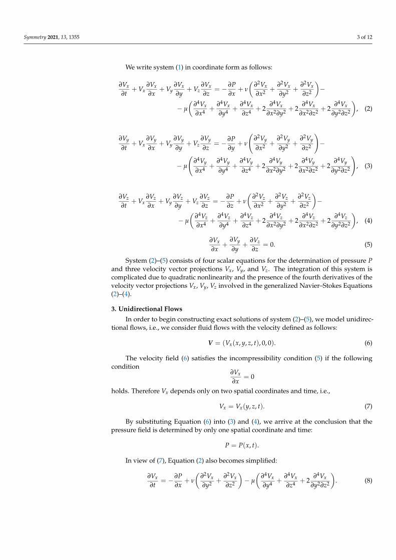
We write system (1) in coordinate form as follows:

∂Vx

∂t+ Vx

∂Vx

∂x+ Vy

∂Vx

∂y+ Vz

∂Vx

∂z= −∂P

∂x+ ν

(∂2Vx

∂x2 +∂2Vx

∂y2 +∂2Vx

∂z2

)−

− µ

(∂4Vx

∂x4 +∂4Vx

∂y4 +∂4Vx

∂z4 + 2∂4Vx

∂x2∂y2 + 2∂4Vx

∂x2∂z2 + 2∂4Vx

∂y2∂z2

), (2)

∂Vy

∂t+ Vx

∂Vy

∂x+ Vy

∂Vy

∂y+ Vz

∂Vy

∂z= −∂P

∂y+ ν

(∂2Vy

∂x2 +∂2Vy

∂y2 +∂2Vy

∂z2

)−

− µ

(∂4Vy

∂x4 +∂4Vy

∂y4 +∂4Vy

∂z4 + 2∂4Vy

∂x2∂y2 + 2∂4Vy

∂x2∂z2 + 2∂4Vy

∂y2∂z2

), (3)

∂Vz

∂t+ Vx

∂Vz

∂x+ Vy

∂Vz

∂y+ Vz

∂Vz

∂z= −∂P

∂z+ ν

(∂2Vz

∂x2 +∂2Vz

∂y2 +∂2Vz

∂z2

)−

− µ

(∂4Vz

∂x4 +∂4Vz

∂y4 +∂4Vz

∂z4 + 2∂4Vz

∂x2∂y2 + 2∂4Vz

∂x2∂z2 + 2∂4Vz

∂y2∂z2

), (4)

∂Vx

∂x+

∂Vy

∂y+

∂Vz

∂z= 0. (5)

System (2)–(5) consists of four scalar equations for the determination of pressure Pand three velocity vector projections Vx, Vy, and Vz. The integration of this system iscomplicated due to quadratic nonlinearity and the presence of the fourth derivatives of thevelocity vector projections Vx, Vy, Vz involved in the generalized Navier–Stokes Equations(2)–(4).

3. Unidirectional Flows

In order to begin constructing exact solutions of system (2)–(5), we model unidirec-tional flows, i.e., we consider fluid flows with the velocity defined as follows:

V = (Vx(x, y, z, t), 0, 0). (6)

The velocity field (6) satisfies the incompressibility condition (5) if the followingcondition

∂Vx

∂x= 0

holds. Therefore Vx depends only on two spatial coordinates and time, i.e.,

Vx = Vx(y, z, t). (7)

By substituting Equation (6) into (3) and (4), we arrive at the conclusion that thepressure field is determined by only one spatial coordinate and time:

P = P(x, t).

In view of (7), Equation (2) also becomes simplified:

∂Vx

∂t= −∂P

∂x+ ν

(∂2Vx

∂y2 +∂2Vx

∂z2

)− µ

(∂4Vx

∂y4 +∂4Vx

∂z4 + 2∂4Vx

∂y2∂z2

). (8)

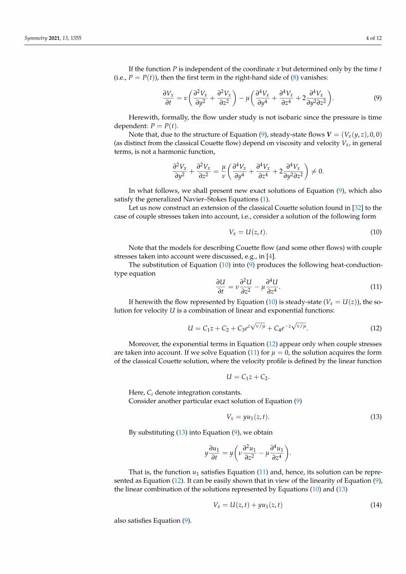
Symmetry 2021, 13, 1355 4 of 12

If the function P is independent of the coordinate x but determined only by the time t(i.e., P = P(t)), then the first term in the right-hand side of (8) vanishes:

∂Vx

∂t= ν

(∂2Vx

∂y2 +∂2Vx

∂z2

)− µ

(∂4Vx

∂y4 +∂4Vx

∂z4 + 2∂4Vx

∂y2∂z2

). (9)

Herewith, formally, the flow under study is not isobaric since the pressure is timedependent: P = P(t).

Note that, due to the structure of Equation (9), steady-state flows V = (Vx(y, z), 0, 0)(as distinct from the classical Couette flow) depend on viscosity and velocity Vx, in generalterms, is not a harmonic function,

∂2Vx

∂y2 +∂2Vx

∂z2 =µ

ν

(∂4Vx

∂y4 +∂4Vx

∂z4 + 2∂4Vx

∂y2∂z2

)6= 0.

In what follows, we shall present new exact solutions of Equation (9), which alsosatisfy the generalized Navier–Stokes Equations (1).

Let us now construct an extension of the classical Couette solution found in [32] to thecase of couple stresses taken into account, i.e., consider a solution of the following form

Vx = U(z, t). (10)

Note that the models for describing Couette flow (and some other flows) with couplestresses taken into account were discussed, e.g., in [4].

The substitution of Equation (10) into (9) produces the following heat-conduction-type equation

∂U∂t

= ν∂2U∂z2 − µ

∂4U∂z4 . (11)

If herewith the flow represented by Equation (10) is steady-state (Vx = U(z)), the so-lution for velocity U is a combination of linear and exponential functions:

U = C1z + C2 + C3ez√

ν/µ + C4e−z√

ν/µ. (12)

Moreover, the exponential terms in Equation (12) appear only when couple stressesare taken into account. If we solve Equation (11) for µ = 0, the solution acquires the formof the classical Couette solution, where the velocity profile is defined by the linear function

U = C1z + C2.

Here, Ci denote integration constants.Consider another particular exact solution of Equation (9)

Vx = yu1(z, t). (13)

By substituting (13) into Equation (9), we obtain

y∂u1

∂t= y

(ν

∂2u1

∂z2 − µ∂4u1

∂z4

).

That is, the function u1 satisfies Equation (11) and, hence, its solution can be repre-sented as Equation (12). It can be easily shown that in view of the linearity of Equation (9),the linear combination of the solutions represented by Equations (10) and (13)

Vx = U(z, t) + yu1(z, t) (14)

also satisfies Equation (9).

Symmetry 2021, 13, 1355 5 of 12

We now add a nonlinear (in the y coordinate) term to (14), i.e., consider a solution ofthe following form

Vx = U(z, t) + yu1(z, t) +y2

2u2(z, t). (15)

Substitute the last sum into (9). Some simple transformations yield

∂U∂t

+ y∂u1

∂t+

y2

2∂u2

∂t= ν

(u2 +

∂2U∂z2 + y

∂2u1

∂z2 +y2

2∂2u2

∂z2

)−

− µ

(∂4U∂z4 + y

∂4u1

∂z4 +y2

2∂4u2

∂z4

).

Applying the method of undetermined coefficients to this equation, we obtain thefollowing system of equations:

∂U∂t

= ν

(u2 +

∂2U∂z2

)− µ

∂4U∂z4 ,

∂u1

∂t= ν

∂2u1

∂z2 − µ∂4u1

∂z4 ,

∂u2

∂t= ν

∂2u2

∂z2 − µ∂4u2

∂z4 .

The latter two equations in this system are equations of the form of (11) and theequation for determining the homogeneous term U in (15) is not isolated any longer.Thus, the consideration of nonlinearity in the variable results in the fact that the solutionrepresented by (15) stops being a superposition of the previously presented solutions.As the power at the y coordinate increases, this tendency holds true. In other words,a unidirectional flow is described by the following exact solution

Vx = U(z, t) +n

∑k=1

yk

k!uk(z, t).

This exact solution, as all those presented in what follows, need to be studied forstability. However, studying for stability questions is not the aim of this paper.

Note that unidirectional flows of non-Newtonian fluids have been studied in manyworks (see, e.g., [33–36] and the references therein).

4. Exact Solutions for Three-Dimensional Flows

In order to study the properties of three-dimensional flows of viscous fluids, one needsto have a reserve of exact solutions to the Navier–Stokes Equations. The exact solutionsinheriting nonlinear properties of the motion equations help to understand better theequations structure in further analytical and numerical integrations [23–25,37–44].

As a preliminary, the exact solution of the system of nonlinear partial Equations (2)–(5)is sought within the Lin–Sidorov–Aristov family [18–20]:

Vx(x, y, z, t) = U(z, t) + xu1(z, t) + yu2(z, t),

Vy(x, y, z, t) = V(z, t) + xv1(z, t) + yv2(z, t),

Vz(z, t) = w(z, t).

(16)

Note that the expressions in Equation (16), they can be treated as the Taylor seriesexpansion of the velocity vector components that is confined to linear terms [37].

Symmetry 2021, 13, 1355 6 of 12

We substitute the class (16) into (2) and immediately ignore the terms containing thesecond and fourth derivatives with respect to the x and y variables since the expressions inEquation (16) linearly depend on these coordinates; this gives

∂(U + xu1 + yu2)

∂t+ (U + xu1 + yu2)

∂(U + xu1 + yu2)

∂x+

+(V + xv1 + yv2)∂(U + xu1 + yu2)

∂y+ w

∂(U + xu1 + yu2)

∂z=

= −∂P∂x

+ ν∂2(U + xu1 + yu2)

∂z2 − µ∂4(U + xu1 + yu2)

∂z4 .

We now make the following simple transformations in this equation by computing thepartial derivatives and combining similar terms at the identical powers of the independentvariables x and y:(

∂U∂t

+ Uu1 + Vu2 + w∂U∂z

)+ x(

∂u1

∂t+ u2

1 + v1u2 + w∂u1

∂z

)+

+y(

∂u2

∂t+ u1u2 + v2u2 + w

∂u2

∂z

)= −∂P

∂x+

(ν

∂2U∂z2 − µ

∂4U∂z4

)+ (17)

+x(

ν∂2u1

∂z2 − µ∂4u1

∂z4

)+ y(

ν∂2u2

∂z2 − µ∂4u2

∂z4

).

The structure of the obtained expression suggests that the pressure should be viewedas a quadratic form of the x and y variables. In other words, we have

P(x, y, z, t) =P0(z, t) + xP1(z, t) + yP2(z, t)+

+x2

2P11(z, t) + xyP12(z, t) +

y2

2P22(z, t).

(18)

Taking into account (18), when the method of undetermined coefficients is applied,Equation (17) splits into the following three equations:

∂U∂t

+ Uu1 + Vu2 + w∂U∂z

= −P1 + ν∂2U∂z2 − µ

∂4U∂z4 ,

∂u1

∂t+ u2

1 + v1u2 + w∂u1

∂z= −P11 + ν

∂2u1

∂z2 − µ∂4u1

∂z4 , (19)

∂u2

∂t+ u1u2 + v2u2 + w

∂u2

∂z= −P12 + ν

∂2u2

∂z2 − µ∂4u2

∂z4 .

Similar operations with the substitution of Equations (16) and (18) into the other twoequations of system (2)–(4) yield, respectively, the following two systems:

∂V∂t

+ Uv1 + Vv2 + w∂V∂z

= −P2 + ν∂2V∂z2 − µ

∂4V∂z4 ,

∂v1

∂t+ u1v1 + v1v2 + w

∂v1

∂z= −P12 + ν

∂2v1

∂z2 − µ∂4v1

∂z4 , (20)

∂v2

∂t+ u2v1 + v2

2 + w∂v2

∂z= −P22 + ν

∂2v2

∂z2 − µ∂4v2

∂z4 ;

∂w∂t

+ w∂w∂z

=− ∂P0

∂z+ ν

∂2w∂z2 − µ

∂4w∂z4 ,

∂P1

∂z= 0,

∂P2

∂z= 0,

∂P11

∂z= 0,

∂P12

∂z= 0,

∂P22

∂z= 0.

(21)

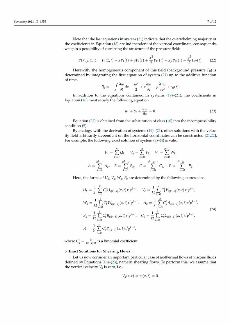
Symmetry 2021, 13, 1355 7 of 12

Note that the last equations in system (21) indicate that the overwhelming majority ofthe coefficients in Equation (18) are independent of the vertical coordinate; consequently,we gain a possibility of correcting the structure of the pressure field:

P(x, y, z, t) = P0(z, t) + xP1(t) + yP2(t) +x2

2P11(t) + xyP12(t) +

y2

2P22(t). (22)

Herewith, the homogeneous component of this field (background pressure P0) isdetermined by integrating the first equation of system (21) up to the additive functionof time,

P0 = −∫

∂w∂t

dz− w2

2+ ν

∂w∂z− µ

∂3w∂z3 + c0(t).

In addition to the equations contained in systems (19)–(21), the coefficients inEquation (16) must satisfy the following equation

u1 + v2 +∂w∂z

= 0. (23)

Equation (23) is obtained from the substitution of class (16) into the incompressibilitycondition (5).

By analogy with the derivation of systems (19)–(21), other solutions with the veloc-ity field arbitrarily dependent on the horizontal coordinates can be constructed [21,22].For example, the following exact solution of system (2)–(4) is valid:

Vx =n

∑k=0

Uk, Vy =n

∑k=0

Vk, Vz =n−1

∑k=0

Wk,

A =n2−n

∑k=0

Ak, B =n2−n

∑k=0

Bk, C =n2−n+1

∑k=0

Ck, P =n2−n+1

∑k=0

Pk.

Here, the forms of Uk, Vk, Wk, Pk are determined by the following expressions:

Uk =1k!

k

∑i=0

CikUi(k−i)(z, t)xiyk−i, Vk =

1k!

k

∑i=0

CikVi(k−i)(z, t)xiyk−i,

Wk =1k!

k

∑i=0

CikWi(k−i)(z, t)xiyk−i, Ak =

1k!

k

∑i=0

Cik Ai(k−i)(z, t)xiyk−i,

Bk =1k!

k

∑i=0

CikBi(k−i)(z, t)xiyk−i, Ck =

1k!

k

∑i=0

CikCi(k−i)(z, t)xiyk−i,

Pk =1k!

k

∑i=0

CikPi(k−i)(z, t)xiyk−i,

(24)

where Cik =

k!(k−i)!i! is a binomial coefficient.

5. Exact Solutions for Shearing Flows

Let us now consider an important particular case of isothermal flows of viscous fluidsdefined by Equations (16)–(23), namely, shearing flows. To perform this, we assume thatthe vertical velocity Vz is zero, i.e.,

Vz(z, t) = w(z, t) = 0.

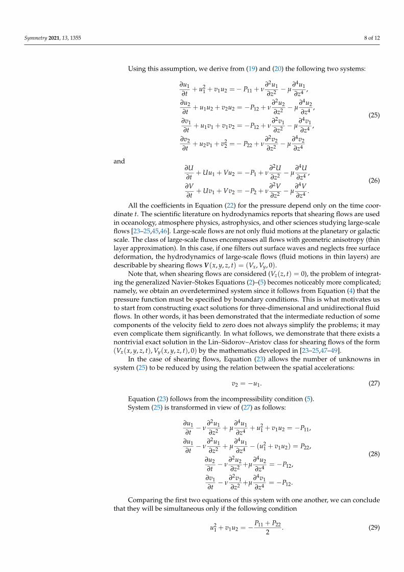
Symmetry 2021, 13, 1355 8 of 12

Using this assumption, we derive from (19) and (20) the following two systems:

∂u1

∂t+ u2

1 + v1u2 =− P11 + ν∂2u1

∂z2 − µ∂4u1

∂z4 ,

∂u2

∂t+ u1u2 + v2u2 = −P12 + ν

∂2u2

∂z2 − µ∂4u2

∂z4 ,

∂v1

∂t+ u1v1 + v1v2 = −P12 + ν

∂2v1

∂z2 − µ∂4v1

∂z4 ,

∂v2

∂t+ u2v1 + v2

2 =− P22 + ν∂2v2

∂z2 − µ∂4v2

∂z4

(25)

and∂U∂t

+ Uu1 + Vu2 = −P1 + ν∂2U∂z2 − µ

∂4U∂z4 ,

∂V∂t

+ Uv1 + Vv2 = −P2 + ν∂2V∂z2 − µ

∂4V∂z4 .

(26)

All the coefficients in Equation (22) for the pressure depend only on the time coor-dinate t. The scientific literature on hydrodynamics reports that shearing flows are usedin oceanology, atmosphere physics, astrophysics, and other sciences studying large-scaleflows [23–25,45,46]. Large-scale flows are not only fluid motions at the planetary or galacticscale. The class of large-scale fluxes encompasses all flows with geometric anisotropy (thinlayer approximation). In this case, if one filters out surface waves and neglects free surfacedeformation, the hydrodynamics of large-scale flows (fluid motions in thin layers) aredescribable by shearing flows V(x, y, z, t) = (Vx, Vy, 0).

Note that, when shearing flows are considered (Vz(z, t) = 0), the problem of integrat-ing the generalized Navier–Stokes Equations (2)–(5) becomes noticeably more complicated;namely, we obtain an overdetermined system since it follows from Equation (4) that thepressure function must be specified by boundary conditions. This is what motivates usto start from constructing exact solutions for three-dimensional and unidirectional fluidflows. In other words, it has been demonstrated that the intermediate reduction of somecomponents of the velocity field to zero does not always simplify the problems; it mayeven complicate them significantly. In what follows, we demonstrate that there exists anontrivial exact solution in the Lin–Sidorov–Aristov class for shearing flows of the form(Vx(x, y, z, t), Vy(x, y, z, t), 0) by the mathematics developed in [23–25,47–49].

In the case of shearing flows, Equation (23) allows the number of unknowns insystem (25) to be reduced by using the relation between the spatial accelerations:

v2 = −u1. (27)

Equation (23) follows from the incompressibility condition (5).System (25) is transformed in view of (27) as follows:

∂u1

∂t− ν

∂2u1

∂z2 + µ∂4u1

∂z4 + u21 + v1u2 = −P11,

∂u1

∂t− ν

∂2u1

∂z2 + µ∂4u1

∂z4 − (u21 + v1u2) = P22,

∂u2

∂t− ν

∂2u2

∂z2 +µ∂4u2

∂z4 = −P12,

∂v1

∂t− ν

∂2v1

∂z2 +µ∂4v1

∂z4 = −P12.

(28)

Comparing the first two equations of this system with one another, we can concludethat they will be simultaneous only if the following condition

u21 + v1u2 = −P11 + P22

2. (29)

Symmetry 2021, 13, 1355 9 of 12

holds.Let us define a linear differential operator Lν,µ by the following formula

Lν,µ =∂

∂t− ν

∂2

∂z2 + µ∂4

∂z4 .

In view of the consistency condition (29), system (28) can be represented as follows:

Lν,µu1 = −P11 − P22

2, Lν,µu2 = −P12, Lν,µv1 = −P12. (30)

Similar results for isobaric two-dimensional and quasi-two-dimensional flows wereobtained earlier (see, e.g., [22,47,50]), but the possibility of the rotational interaction of fluidparticles was not then taken into account. Herewith, system (30) generalizes the resultsreported in [47–49] and it can be reduced to them by passing to the limit as µ→ 0 in theexpression for the operator Lν,µ:

Lν,0 =∂

∂t− ν

∂2

∂z2 .

Note that the consistency condition (29) for the overdetermined system ofEquations (25)–(27) can be obtained on other grounds. Let us write the Navier–Stokesequations (2)–(4) for shearing flows as follows:

∂Vx

∂t+ Vx

∂Vx

∂x+ Vy

∂Vx

∂y= −∂P

∂x+ ν

(∂2Vx

∂x2 +∂2Vx

∂y2 +∂2Vx

∂z2

)−

− µ

(∂4Vx

∂x4 +∂4Vx

∂y4 +∂4Vx

∂z4 + 2∂4Vx

∂x2∂y2 + 2∂4Vx

∂x2∂z2 + 2∂4Vx

∂y2∂z2

), (31)

∂Vy

∂t+ Vx

∂Vy

∂x+ Vy

∂Vy

∂y= −∂P

∂y+ ν

(∂2Vy

∂x2 +∂2Vy

∂y2 +∂2Vy

∂z2

)−

− µ

(∂4Vy

∂x4 +∂4Vy

∂y4 +∂4Vy

∂z4 + 2∂4Vy

∂x2∂y2 + 2∂4Vy

∂x2∂z2 + 2∂4Vy

∂y2∂z2

). (32)

These equations are closed by the incompressibility condition

∂Vx

∂x+

∂Vy

∂y= 0. (33)

We differentiate Equation (31) with respect to the variable x and Equation (32) withrespect to y and add up the obtained expressions. Some simple transformations andthe use of the incompressibility condition (33) result in the following relationship (theconsistency condition):

∂Vx

∂y∂Vy

∂x− ∂Vx

∂x∂Vy

∂y= −1

2

(∂2P∂x2 +

∂2P∂y2

). (34)

The particular case of the condition represented by Equation (34) for isobaric flowswas obtained in [22].

Symmetry 2021, 13, 1355 10 of 12

Substituting expressions (16) and (18) into Equation (34), we obtain

∂(U + xu1 + yu2)

∂y· ∂(V + xv1 + yv2)

∂x− ∂(U + xu1 + yu2)

∂x· ∂(V + xv1 + yv2)

∂y=

= −12

(∂2

∂x2 +∂2

∂y2

)(P0 + xP1 + yP2 +

x2

2P11 + xyP12 +

y2

2P22

).

Elementary transformations for calculating partial derivatives produce thefollowing relation

u2v1 − u1v2 = −P11 + P22

2.

Finally, by substituting Equation (27) into the latter equation, we arrive at the consis-tency condition (29).

By analogy with the results reported in [22], the class of exact solutions (16) forsystem (19)–(21) can be expanded. Note the following velocity field

V(i)x =

n

∑k=0

U(i)k (z, t)

yk

k!, V(i)

y = V(i)(z, t)

and the pressure field

P(x, y, z, t) = P0(z, t) + xP1(t) + yP2(t) +x2

2P11(t) + xyP12(t) +

y2

2P22(t)

satisfy the reduced Navier–Stokes Equations system and the incompressibility condition,i.e., system (25)–(27). If a rotational transformation is performed for the coordinates andvelocities according to the following rule:

x −→ x cos ϕ− y sin ϕ, y −→ x sin ϕ + y cos ϕ,

Vx −→ Vx cos ϕ−Vy sin ϕ, Vy −→ Vx sin ϕ + Vy cos ϕ,

then we obtain a family of exact solutions of the form (24) with a nonlinear dependence ontwo horizontal coordinates (the x and y coordinates).

6. Conclusions

The paper has presented families of exact solutions to the Navier–Stokes Equationsfor describing viscous fluid flows with rotational interaction of fluid particles taken intoaccount. Models describing unidirectional vertical vortex flows have been separatelydiscussed. The class proposed for such flows is characterized by a polynomial dependenceof velocity on one of the horizontal coordinates. The polynomial can be of any order; thecoefficients in the polynomial representation are arbitrarily related to the vertical coordinateand time. It has been demonstrated that quadratic and higher-power polynomial solutionscannot be obtained by superposition of lower-power solutions.

The solution families for describing three-dimensional flows have been considered.The Lin–Sidorov–Aristov family of exact solutions is chosen as the basic class and extendedto the case of arbitrary-power dependences of the velocity field on the horizontal coordi-nates. The case of shearing flows has been separately discussed. It has been shown that thesystem of constitutive relations for spatial accelerations is reducible to a system of operatorequations for which the solutions must satisfy a consistency condition of a special form.The consistency condition itself is derived in several ways.

It has also been shown that the proposed classes are a generalization of our previousresults. Moreover, in the passage to the limit, which enables one to ignore the possibilityof rotational interaction among fluid particles, these classes coincide with previouslypublished results.

Symmetry 2021, 13, 1355 11 of 12

Author Contributions: Conceptualization, N.V.B. and E.Y.P.; methodology, N.V.B. and E.Y.P.; writing—original draft preparation, E.S.B., N.V.B. and E.Y.P.; writing—review and editing, E.S.B., N.V.B. andE.Y.P. All authors have read and agreed to the published version of the manuscript.

Funding: This research received no external funding.

Institutional Review Board Statement: Not applicable.

Informed Consent Statement: Not applicable.

Data Availability Statement: Not applicable.

Conflicts of Interest: The authors declare no conflict of interest.

References1. Landau, L.D.; Lifshitz, E.M. Course of Theoretical Physics. Volume 6. Fluid Mechanics; Pergamon Press: Oxford, UK, 1987.2. Temam, R. Navier–Stokes Equations. Theory and Numerical Analysis; North-Holland: Amsterdam, The Netherlands, 1979.3. Aero, E.L.; Bulygin, A.N.; Kuvshinskii, E.V. Asymmetric hydromechanics. J. App. Math. Mech. 1965, 29, 333–346. [CrossRef]4. Stokes, V.K. Couple stresses in fluids. Phys. Fluids. 1966, 9, 1709–1715. [CrossRef]5. Stokes, V.K. Theories of Fluids with Microstructure. An Introduction; Springer: Berlin, Germany, 1984. [CrossRef]6. Stokes, V.K. Effects of couple stresses in fluids on hydromagnetic channel flows. Phys. Fluids. 1968, 11, 1131–1133. [CrossRef]7. Stokes, V.K. On some effects of couple stresses in fluids on heat transfer. J. Heat Transfer. 1969, 91, 182–184. [CrossRef]8. Devakar, M.; Iyengar, T.K.V. Stokes’ problems for an incompressible couple stress fluid. Nonlinear Anal. Model. Control. 2008, 13,

181–190. [CrossRef]9. Eringen, A.C. Simple microfluids. Int. J. Eng. Sci. 1964, 2, 205–217. [CrossRef]10. Eringen, A.C.; Suhubi, E.S. Nonlinear theory of simple micro-elastic solids. Int. J. Eng. Sci. 1964, 2, 189–203. [CrossRef]11. Eringen, A.C. Theory of micropolar fluids. J. Math. Mech. 1966, 16, 1–18. [CrossRef]12. Toupin, R.A. Elastic materials with couple-stresses. Arch. Ration. Mech. Anal. 1962, 11, 385. [CrossRef]13. Eremeev, V.A.; Zubov, L.M. Fundam. Mech. A Viscoelastic Micropolar Fluid; SSC RAS: Rostov, Russia, 2009. (In Russian)14. Joseph, S.P. Some exact solutions for incompressible couple stress fluid flows. Malaya J. Mat. 2020, 648–652. [CrossRef]15. Cosserat, E.; Cosserat, F. Théorie des Corps Déformables; A. Hermann et Fils: Paris, France, 1909.16. Ahmad, F.; Nazeer, M.; Ali, W.; Saleem, A.; Sarwar, H.; Suleman, S.; Abdelmalek, Z. Analytical study on couple stress fluid in an

inclined channel. Sci. Iran. 2021. [CrossRef]17. Srinivas, J.; Ramana Murthy, J.V. Thermal analysis of a flow of immiscible couple stress fluids in a channel. J. Appl. Mech. Tech.

Phys. 2016, 57, 997–1005. [CrossRef]18. Lin, C.C. Note on a class of exact solutions in magneto-hydrodynamics. Arch. Ration. Mech. Anal. 1957, 1, 391–395. [CrossRef]19. Sidorov, A.F. Two classes of solutions of the fluid and gas mechanics equations and their connection to traveling wave theory.

J. Appl. Mech. Tech. Phys. 1989, 30, 197–203. [CrossRef]20. Aristov, S.N. Eddy Currents in Thin Liquid Layers. Ph.D. Thesis, Institute of Automation and Control Processes, Vladivostok,

Russia, 1990. (In Russian)21. Prosviryakov, E.Y. New class of exact solutions of Navier–Stokes Equations with exponential dependence of velocity on two

spatial coordinates. Theor. Found. Chem. Eng. 2019, 53, 107–114. [CrossRef]22. Zubarev, N.M.; Prosviryakov, E.Y. Exact solutions for layered three-dimensional nonstationary isobaric flows of a viscous

incompressible fluid. J. Appl. Mech. Tech. Phys. 2019, 60, 1031–1037. [CrossRef]23. Burmasheva, N.V.; Prosviryakov, E.Y. Exact solution of Navier–Stokes Equations describing spatially inhomogeneous flows of a

rotating fluid. Tr. Instit. Mat. I Mekh. UrO RAN. 2020, 26, 79–87. (In Russian) [CrossRef]24. Burmasheva, N.V.; Prosviryakov, E.Y. A class of exact solutions for two-dimensional equations of geophysical hydrodynamics

with two Coriolis parameters. Izv. Irkutsk. Gos. Univ. Ser. Mat. 2020, 32, 33–48. (In Russian) [CrossRef]25. Burmasheva, N.V.; Prosviryakov, E.Y. Isothermal layered flows of a viscous incompressible fluid with spatial acceleration in the

case of three Coriolis parameters. DReaM 2020, 3, 29–46. (In Russian) [CrossRef]26. Öz, Y. Rigorous investigation of the Navier–Stokes momentum equations and correlation tensors. AIP Adv. 2021, 11, 055009.

[CrossRef]27. Münch, I.; Neff, P.; Madeo, A.; Ghiba, I.-D. The modified indeterminate couple stress model: Why Yang et al.’s arguments

motivating a symmetric couple stress tensor contain a gap and why the couple stress tensor may be chosen symmetric nevertheless.Z. Angew. Math. Mech. 2017, 97, 1524–1554. [CrossRef]

28. Hadjesfandiari, A.R.; Dargush, G.F. Evolution of Generalized Couple-Stress Continuum Theories: A Critical Analysis. arXiv 2014,arXiv:1501.03112.

29. Reggiani P.; Sivapalan, M.; Hassanizadeh, S.M.; Gray, W.G. Coupled equations for mass and momentum balance in a streamnetwork: Theoretical derivation and computational experiments. Proc. R. Soc. Lond. A. 2001, 457, 157–189. [CrossRef]

30. Ladyzhenskaya, O.A. On nonstationary Navier–Stokes Equations. Vestn. Leningr. Univ. 1958, 19, 9–18.

Symmetry 2021, 13, 1355 12 of 12

31. Ladyzhenskaya, O.A. On some gaps in two of my papers on the Navier–Stokes Equations and the way of closing them. J. Math.Sci. 2003, 115, 2789–2791. [CrossRef]

32. Couette, M. Études sur le frottement des liquids. Ann. Chim. Phys. 1890, 21, 433–510.33. Baranovskii, E.S.; Artemov, M.A. Steady flows of second-grade fluids in a channel. Vestn. S. Peterb. Univ. Prikl. Mat. Inf. Protsessy

Upr. 2017, 13, 342–353. (In Russian) [CrossRef]34. Domnich, A.A.; Baranovskii, E.S.; Artemov, M.A. A nonlinear model of the non-isothermal slip flow between two parallel plates. J.

Phys. Conf. Ser. 2020, 1479, 012005. [CrossRef]35. Fetecau, C.; Vieru, D.; Abbas, T.; Ellahi, R. Analytical solutions of upper convected Maxwell fluid with exponential dependence of

viscosity under the influence of pressure. Mathematics 2021, 9, 334. [CrossRef]36. Fetecau, C.; Vieru, D. Symmetric and non-symmetric flows of Burgers’ fluids through porous media between parallel plates.

Symmetry 2021, 13, 1109. [CrossRef]37. Aristov, S.N.; Knyazev, D.V.; Polyanin A.D. Exact solutions of the Navier–Stokes Equations with the linear dependence of velocity

components on two space variables. Theor. Found. Chem. Eng. 2009, 43, 642–662. [CrossRef]38. Molchanov, A.M. Numerical Methods for Solving the Navier–Stokes Equations. OSF Preprints. 2019. Available online: https:

//osf.io/zf3j2/ (accessed on 20 June 2021).39. Chen, Z.J.; Li, Z.Y.; Xie,W.L.; Wu, X.H. A two-level variational multiscale meshless local Petrov–Galerkin (VMS-MLPG) method for

convection-diffusion problems with large Peclet number. Comput. Fluids. 2017, 1, 1–10.40. Li, S. Time Advancement of the Navier–Stokes Equations: P-adaptive exponential methods. J. Flow Cont. Meas. Visual. 2020, 8,

63–76. [CrossRef]41. Li, S.-J.; Wang, Z.J.; Ju, L.; Luo, L.-S. Fast time integration of Navier–Stokes Equations with an exponential-integrator scheme. In

Proceedings of the AIAA Aerospace Sciences Meeting, Kissimmee, FL, USA, 8–12 January 2018. [CrossRef]42. Li, L.; Yang, Z.; Dong, S. Numerical approximation of incompressible Navier–Stokes Equations based on an auxiliary energy

variable. J. Comput. Phys. 2019, 388, 1–22. [CrossRef]43. Chen, H.; Sun, S.; Zhang, T. Energy stability analysis of some fully discrete numerical schemes for incompressible Navier–Stokes

Equations on staggered grids. J. Sci. Comput. 2018, 75, 427–456. [CrossRef]44. Dong, S. Multiphase flows of N immiscible incompressible fluids: A reduction-consistent and thermodynamically-consistent

formulation and associated algorithm. J. Comput. Phys. 2018, 361, 1–49. [CrossRef]45. Ingel, L.K.; Kalashnik, M.V. Nontrivial features in the hydrodynamics of seawater and other stratified solutions. Phys. Usp. 2012,

55, 356–381. [CrossRef]46. Beskin, V.S. Axisymmetric steady flows in astrophysics. Phys. Usp. 2003, 46, 1209–1214. [CrossRef]47. Aristov, S.N.; Prosviryakov, E.Y. Inhomogeneous Couette flow. Rus. J. Nonlin. Dyn. 2014, 10, 177–182. (In Russian) [CrossRef]48. Aristov, S.N.; Prosviryakov, E.Y. Stokes waves in vortical fluid. Rus. J. Nonlin. Dyn. 2014, 10, 309–318. (In Russian) [CrossRef]49. Aristov, S.N.; Prosviryakov, E.Y. Nonuniform convective Couette flow. Fluid Dyn. 2016, 51, 581–587. [CrossRef]50. Shmyglevskii, Y.D. On isobaric planar flows of a viscous incompressible liquid. USSR Comput. Math. Math. Phys. 1985, 25, 191–193.

[CrossRef]