1

From Euler to Navier-Stokes: A spatial analysis of conceptual changes in 19th-

century fluid dynamics

Graciana Petersen

University of Hamburg

Center for Earth System Research and Sustainability

Bundesstrasse 55

20146 Hamburg, Germany

gracianapetersen@gmx.de

Frank Zenker

Lund University

Department of Philosophy & Cognitive Science

Kungshuset, Lundagård

22 222 Lund, Sweden

frank.zenker@fil.lu.se

Abstract: This article provides a spatial analysis of the conceptual framework of fluid

dynamics during the 19th century, focusing on the transition from the Euler Equation

to the Navier-Stokes Equation. A dynamic version of Gärdenfors’s (2000) theory of

conceptual spaces is applied which distinguishes five types of changes (addition and

deletion of special laws; change of metric; change in importance; change in

separability; addition and deletion of dimensions). The case instantiates all types but

the deletion of dimensions. We also provide a new view upon limiting case reduction

at the conceptual level that clarifies the relation between the predecessor and

2

successor conceptual framework. The 19th-century development of fluid dynamics is

argued to be an instance of normal science development.

Keywords: conceptual change, conceptual spaces, dimensional analysis, Euler

equation, fluid dynamics, fluid mechanics, limiting case reduction, normal science,

Navier-Stokes equation, theory change

1. Introduction

This article applies a diachronic version of conceptual spaces (Gärdenfors, 2000) to

reconstruct the dynamics of the conceptual framework of fluid dynamics during the

19th century, and provides a geometric analysis of dimensional quantities in the

transition from the Euler Equation (EE) to the Navier-Stokes Equation (NSE). The

case study shows that conceptual spaces accurately describe the changes from the EE

to the NSE, and thus supports the conjecture that this tool can map yet more complex

historical cases.1 Absent a rigorous proof of the exact formal relation between the EE

1 Our conjectures are based on several observations. First, conceptual spaces have

already proven useful for the description of scientific theories in other cases

(Gärdenfors & Zenker, 2011; 2013; Zenker & Gärdenfors, 2013; 2014). Further,

conceptual spaces are already used—alas, largely unconsciously—in many real

world applications; consultancies, for instance, apply a simplified version of

conceptual spaces as a pragmatic tool to describe and solve complex problems, thus

in theory-choice. Finally, conceptual spaces benefit from their proximity to

mathematics, thus enriching scientific communication and contributing to the

learning landscape.

3

and the NSE,2 conceptual spaces prove useful as a pragmatic and visual tool. As is

the case for scientists, this may reveal new perspectives to scholars of science;

dimensional change, for instance, may go along with innovations in problem-solving

(see Sect. 3). Furthermore, insights into limiting case reduction can be compared to

what is available at the symbolic level of representation, where such reductions are

standardly treated (see Sect. 5).

We begin with an outline of conceptual spaces and introduce five types of

changes by example (Sect. 2). This typology is applied to the conceptual framework

of fluid dynamics in the 19th century (Sect. 3 and Sect. 4), and a summary of salient

changes is provided (Sect. 5). Insights into limiting case reduction and more general

considerations are discussed (Sect. 6). Sect. 7 offers our conclusions.

2. Conceptual Spaces as a Reconstructive Tool

Empirical theories are formulated against the background of a scientific conceptual

framework that provides the magnitudes on which applications of theoretical models

to real world phenomena rely. Such magnitudes are here reconstructed as collections

of dimensions and their inter-relations, that is, as conceptual spaces. While a

conceptual space corresponds to a set with a certain structure, the introduction of

quality dimensions, being not native to set theory, reflects a geometrical

understanding of the objects in the set. (See Gärdenfors & Zenker, 2011, and Zenker

& Gärdenfors, 2013 for a comparison with reconstructions in Sneed/Stegmüller

structuralism.) Schematically, an empirical theory, T, is formulated against a

conceptual framework, F, which is reconstructed as a conceptual space, S.

2 Known as one of the millennium problems, the challenge is to prove the existence

and smoothness of the NSE (Fefferman, 2014).

4

2.1 Conceptual Spaces

The basic components of a conceptual space are its dimensions. This notion can be

taken literally. The assumption is that each dimension is endowed with a certain

geometrical structure. In some cases, these are topological features or orderings. In

the scientific case, the dimensions are determined by the variables presumed in a

theory. To illustrate, consider mass [M], length [L], and time [T], as used in

Newtonian mechanics. The first two have a zero point, and their values are chosen

from the non-negative real numbers, while values for time can be chosen from the

full real number line.

Dimensions are taken to be independent of symbolic representations. After

all, one can represent the qualities of objects by (partial) vectors without presuming

an explicit object language in which these qualities are expressed. Consequently, also

the limiting case relation between a predecessor and a successor theory can be treated

independently of symbolic representation. As is shown below, when a predecessor

conceptual framework F is a limiting case of a successor framework F*, then the

space F is a restricted hyperplane of F*. Furthermore, the meaning of scientific terms

such as mass or time is taken to be independent of their ontology. Rather, meaning is

determined by the role in the conceptual framework and the methods by which a

magnitude can be measured (Roche, 1998).

2.2 Separable and Integral Dimensions

Dimensions can be sorted into domains, defined via a distinction between integral

and separable dimensions (Melara, 1992; Maddox, 1992). Dimensions are said to be

integral if, to describe an object fully, one cannot assign it a value on one dimension

without giving it some value on another. For instance, one cannot assign the pitch of

5

a sound without assigning its loudness, so pitch and loudness are integral

dimensions. Dimensions that are not integral are separable, e.g., the volume of an

object in the domain of space and its hue in the color domain. For scientific theories,

the distinction can also be made in terms of invariance transformations as one “may

define a scale as a class of measurement procedures having the same transformation

properties” (Suppes, 2002, p. 114; see pp. 97−128), where “measurement procedure”

thus denotes the pragmatic aspect of mathematical invariance. For instance, mass is

separable from everything else in Newtonian theory, but not from energy in special

relativity. It is part of the meaning of “integral dimensions” that the dimensions share

a metric.

More precisely, a theory domain is the set of integral dimensions separable

from all other dimensions: Domain C is separable from D in a theory if and only if

(iff) the invariance transformations of the dimensions in C do not involve any

dimension from D; and the dimensions of a domain C are integral iff their invariance

class does not involve any other dimension.

For a given set of dimensions, furthermore, the choice of domains need not be

unique as the organization of dimensions into domains depends on the definition of

separability. In the literature, such organization principles tend to be based either on

a theoretical motivation (e.g., via transformation classes) or a practical one (e.g., via

measurement procedures).3 In any case, the set of domains then depends on the

choice of dimensions, notably the basic ones given by the International System of

3 A practical criterion for identifying domains can thus be connected to the

measurement procedures for the domains, for instance in experimental research.

But domains may also be identified mathematically, if only to ask later whether

such pure distinctions can be supplied with feasible measurement methods.

6

Units (SI-units), and the choice of useful derived dimensions. Ontological

considerations have historically informed such choices; the present notion of

basicness, however, is a conventional one.

2.3 Dimensional Analysis

Analyzing an empirical theory, its scientific conceptual framework always comes out

as a collection of domains. Studying the dynamic case results in a diachronic version

of dimensional analysis. Macagno (1971) and Martins (1981) provide a brief

historical account. Dimensional analysis generally shifts attention away from axioms

and special laws, and towards the conceptual framework itself. Provided the meaning

of a scientific concept is determined by its constitutive dimensions and its

measurement procedures, axioms and special laws now express constraints on the

distribution of points over the dimensions that are presupposed in a theory.

Technically, laws are hypersurfaces (aka hyperplanes) to a space. Newton’s second

law of motion, for instance, restricts points to lie on the hyperplane spanned by

F=ma (Gärdenfors, 2000, p. 216). This equation connects all eight dimensions of the

Newtonian framework: mass (1D), time (1D), space (3D), force (3D).4

As all dimensions are treated equally, domains need not consist only of

fundamental dimensions in the sense of “fundamental measurement magnitudes.” So

fundamental vs. derived magnitude can be a pragmatic distinction only that need not

square with epistemological or ontological commitments as to which dimensions are

primitive or irreducible. A distinction such as Sneed’s (1971) between T-theoretical

4 Strictly, forces need not be introduced separately; they “fall out” according to

Newton’s F=ma. So forces do not form a domain in the sense of Sect. 2.2.

7

terms and T-non-theoretical ones generally remains possible.5 Below, the term

‘dimension’ is employed irrespective of whether a variable is reconstituted in a

single domain, or whether variables combine elements of several domains. A length,

for instance, is referred to as [L], involving one domain (space), while velocity is

referred to as [LT-1], with two domains (space, time).

2.4 Five Types of Changes

Changes to a theoretical framework divide into five analytical types, here presented

in order of increasing severity (see Gärdenfors & Zenker, 2011; 2013; Zenker &

Gärdenfors, 2013; 2014). A so-called scientific revolution (Kuhn, 1970) falls mostly

under the fifth type, as the replacement of dimensions.

Addition and Deletion of Special Laws Special laws may be added or deleted

from a theory, but endorsing fewer or more of them remains comparatively

unimportant as long as the conceptual framework remains stable. Changes to a

special law thus maintain the conceptual space, but differentially restrict the

distribution of points over the dimensions (see Sect. 2.3).

Change of Scale or Metric Dimensions are endowed with different metrics or

scales. Stevens (1946) distinguished four types—nominal, ordinal, interval, and

ratio—ordered according to levels of measurement (see Krantz et al., 1971; 1989;

1990), the next level showing less mathematical invariance than the preceding one.

Relative to a stable dimensional framework, “changing scale” admits of differentially

precise expressions of a theory’s empirical theory, e.g., the change from macroscopic

5 For Sneed, a T-theoretical dimension is one whose value cannot be determined

without applying the theory T. Mass and force thus become T-theoretical

dimensions in Newtonian mechanics (Sneed, 1971).

8

fluid dynamics, where continuous scaling is assumed, to molecular fluid dynamics,

assuming a discrete structure (see Sect. 3).

Change in the Importance of Dimensions Changes in importance leave a

theory’s empirical content intact; they rather depend on attitudes and commitments

regarding fundamental vs. derived dimensions that, for various reasons, change as

science develops. Separating forces into long range and short range ones, for

instance, sees specific forces gain importance as explanatory mechanisms, or causes,

of fluids in motion, making the theory less idealized (see Sect. 3). Substitution of

extant variables by more sophisticated ones may generally be viewed as an

innovation in problem-solving. A second example is density [ML-3] on a

macroscopic view which assumes a continuously spread mass (the fluid) and treats

density mostly as an average quantity, constant throughout the volume, thus

evidencing the factual distribution of densities to be unimportant. When the

Boltzmann-Equations apply to fluid dynamics on a microscopic view, in contrast,

then the exact constitution of densities gain in importance. So only when density is

unimportant can a macroscopic and a microscopic treatment be unified, in turn

spelling out an assumption for limiting case reduction to become feasible (see Sect.

6).6 A final example is the increase in the importance of length [L] and time [T].

Fluids in motion describe a vector field of velocities [LT-1], i.e., displacements over

time intervals, with a velocity vector assigned to each point of the 3D space (given

6 Standardly, the unification of microscopic particle dynamics with macroscopic

fluid dynamics proceeds via a limiting case demonstration (assuming infinitely

many particles), and has the microscopic theory collapse into the macroscopic

one. So density is never completely unimportant, but under a macroscopic view

one can disregard its complexity.

9

by three numbers taking the units of velocities [LT-1], and another three taking the

units of space [L]), such that velocity recurs to differences expressible on the extant

quality dimensions [L] and [T]. Apart from constituting [LT-1], then, [L] and [T] are

also separable domains (see Sect. 2.2).

Change in the Separability of Dimensions As stated in Sect. 2.2, a dimension

of a domain C is integral iff its invariance class does not involve other dimensions.

Changes in separability are comparatively radical, because they entail a change in

measurement methods. To give a genuinely hypothetical example, if mass were to

depend on charge, then traditional measurement procedures for mass could no longer

be used. An example from thermodynamics is heat which lost its independent status

when Boltzmann functionalized differences in temperature as differences in mean

kinetic energy (Chang, 2004). Such changes are typically connected with a

unification of two theories, and they may go along with to the addition of a new

variable, e.g., the addition of a fluid’s viscosity [ML-1T-1]: the deviatoric stress tensor

(a force per area) came, on empirical grounds, to depend on the velocity gradient of a

moving fluid (one-dimensional case:

, u=velocity, x=direction of derivation), with

the linear factor now linking velocity [LT-1] with forces [ML3T-1] being interpreted

as the new material property viscosity (see Sect. 3).

Addition and Deletion of Dimensions The most extreme change occurs when

a dimension is added to, or deleted from, a conceptual framework. An example is the

addition of the viscosity term to the Navier-Stokes Equation. In contrast, the deletion

of dimensions could be avoided, rendering the EE-to-NSE transition an instance of

conservative induction where prior successful applications are retained (see Sect. 5).

10

3. The Conceptual Development of 19th

-Century Fluid Dynamics

We now apply the above typology to the conceptual framework of 19th-century fluid

dynamics to describe the transition from the Euler Equation (EE) to the Navier-

Stokes Equation (NSE). A time-line is provided in the appendix (Table 1). We

exclude developments such as boundary layer theory (Prandtl, 1904) or 20th-century

research on turbulence (e.g., Taylor, Richardson and Kolmogorov). Throughout the

19th century, the Navier-Stokes Equation has been derived on at least five occasions,

at times independently: C.L.M.H. Navier derives the NSE, in 1821, as the viscosity

extension of the Euler Equation. In 1829, S.D. Poisson provides a new derivation of

the NSE, inspired by Laplace’s molecular physics, mentioning neither Navier nor

Cauchy’s 1821 elasticity theory. In 1837, A.B. de Saint-Venant provides a derivation

of the NSE. Independently, H. Helmholtz derives the NSE, in 1859, based on internal

friction. The NSE counts as established with Maxwell’s kinetic theory of gases, in

1866, with the review of H. Lamb, and studies on turbulent flow by Reynolds and

Boussinesq during the 1880s (Darrigol, 2005; Tokaty, 1971).

Terms such as d’Alembert’s and Lagrange’s virtual velocities, Navier’s life

forces (kinetic energy), or quantity of action (work) are no longer used today or are

regarded as irrelevant for modern fluid dynamics. With mathematical developments,

also experimental practices changed. The use of wind tunnels and water channels, for

instance, became standard. More recently, models of fluid dynamics have gained

societal relevance as they are being applied, among others, to predict atmospheric

flow, to determine air pollution zones, to assess wind energy potentials, and to

forecast smoke movement in emergency responses. Numerous further applications

are found in industrial engineering and medicine (Petersen, 2013).

The EE-to-NSE transition widely counts as the main 19th-century

achievement in the development towards present day fluid dynamics. Below, the EE

11

are treated as the core of fluid mechanics, and the NSE as the core of modern fluid

dynamics. We first turn to fluid mechanics and the EE. Our starting point is the

continuum hypothesis (CH) and we will move via classical mechanics to the EE and

on to the NSE. We view Euler as the founder of fluid mechanics (Tokaty, 1971), who

translated fluids as physical objects into mathematical (geometrical) objects. At each

step, we provide a dimensional reconstitution of the conceptual space of fluid

mechanics as it develops into fluid dynamics. In Sect. 5, limiting case reduction is

discussed on a spatial (geometrical) view, which provides insights into constructing a

successor conceptual framework F* from its predecessor F, thus clarifying what it

means, geometrically speaking, that a theory formulated in F* collapses into one

formulated in F.

The foundation for the modern treatment is classical mechanics. The latter

introduced force [MLT-2] and mechanical equilibrium to fluid dynamics. Forces were

subsequently split into long range and short range forces that, respectively, act on a

volume element and its surface. The continuum hypothesis (CH) constitutes the

fundamental assumption and also the historical basis of fluid mechanics.

3.1. The Continuum Hypothesis

The continuum hypothesis (CH) states that the distance between a liquid’s molecules

is much larger than their individual size. On observational grounds, a fluid’s

macroscopic behavior is treated as if it were continuous, so not made up of particles.

Its discrete structure “idealized away,” mathematical points can characterize the

fluid. Modern fluid dynamics thus allows calculating the trajectory, that is, the

history of the movements of “fluid particles,” where these are understood as volume-

less parts of a continuous fluid, while at the microscopic level nothing will be found

to correspond to the trajectory of such volume elements. Endorsing the CH therefore

12

amounts to accepting that the true dynamics of fluid particles are not considered.7

Note that the CH is necessary to establish the NSE.

A systematically minimal, and historically accurate way to introduce the CH

into the conceptual space of fluid dynamics consists in postulating mass density as an

amorphous one-dimensional (1D) quality of materials and the volume domain [L3],

e.g., the 3D space, and defining a body’s mass [M] as the product of density [ML-3]

and volume [L3]. This is similar to how Newton defined mass in terms of density and

volume at the beginning of Principia, while density then played no further role.

3.2 Adding Body and Long Range Forces as New Dimensions

Above, we had seen classical mechanics being applied to the “continuitized” fluid

object to describe forces that act on it. When long range forces are now distinguished

from short range forces, then the fluid’s molecules are assumed to form an idealized

continuous matter, equally distributed within the volume element (δV). This amounts

7 Microscopic particle dynamics can be accounted for by the Boltzmann equation,

(Hirschfelder et al., 1965); also the Einstein kinetic model or other stochastic

processes may be considered for molecular motions (Einstein, 1905;

Smoluchowski, 1906; Erdös, 2012). Moreover, a linear Boltzmann equation can

be formulated that couples Boltzmann’s particle distribution function with the

so-called “random jump process” on the sphere of velocities. A key difficulty

pertains to the combination of microscopic and macroscopic fluid scales in the

collision of reversible and irreversible processes, since Hamiltonian mechanics

(i.e., classic mechanics) is reversible in time and deterministic, while the

Boltzmann equation is irreversible. The result is an inevitable loss of

information at a macroscopic scale (Erdös, 2012, p. 7).

13

to a change in metric, i.e., a change in the topography, of density: from discrete to

continuous. This change is paired with the addition of the space domain [L3], for

volume, thus introducing the mass dimensions [M] to the basic space, which consists

of mass-density [ML-3] and volume [L3], as above.

The dimensions of force [ML3T-1], furthermore, are added and then split into

more specific dimensions for long range and short range forces. The former include

gravity, electromagnetic forces, as well as fictitious ones such as the centrifugal

forces brought about by the global movement of the continuous space. Long range

forces, also called volume forces or body forces, act equally on all matter contained

in a fluid volume, and are proportional to the volume and the density of the fluid.

Force being a function of space and time, proportional to the density and size of the

volume element, the total body force that, at time t, impacts on the volume δV with

density ρ associated to the spatial position x is now given by:

Total body force = F(x, t) ρ δV (1)

F yields an acceleration of the fluid volume element. The link to Newton’s

second law, F=ma, may now be obvious: the product ρ δV gives the mass, m, of the

volume element, and F(x, t) denotes the acceleration, a. The conceptual space now

consists of either three or four domains: 3D force, 1D density, and 3D space, or the

foregoing plus 1D time. Strictly, time is not needed, and space may also be

considered as being one dimensional.8 Closer to realistic intuitions, space can be

reconstituted as the three dimensional domain ℝ3, which is a “flat” vector space

8 Such a reduction of spatial dimensionality, here from three dimensions to one,

can simplify a problem and is often useful in computational modeling.

14

(Cartesian coordinate system). So the vector spaces add a metric onto the hitherto

amorphous space.

Unlike long range ones, short range forces have molecular origin. They are

assumed to “decrease extremely rapidly with increase of distance between interacting

elements, and are applicable only when that distance is of the order of the separation

of molecules of the fluid” (Batchelor, 1970, p. 7). Within a volume element, then,

collisions between molecules can be neglected when matter is assumed to be

distributed continuously and equally. This is still consistent with the CH. A

conceptual novelty consists in considering the interaction with materials that deform

the volume element by acting from its outside. Such deformations are treated as an

effect of a surface force, an assumption that is transferred from the continuum

mechanics of solids. Surface forces act proportionally to a given surface, δA, and are

directed. The surface force on δA, acting in a direction perpendicular to the surface at

time t for a fluid element at position x, is given by:

Σ(n, x, t) δA (2)

The surface force per unit area, also called stress, is an odd function9 of the

vector pointing in a perpendicular direction to the surface, n, given by:

Σ(−n, x, t) δA = −Σ(n, x, t) δA (3)

9 Definition: Let f (x) be a real-valued function of a real variable. Then f is odd if

−f(x)=f(−x) for all x in R.

15

For the total deforming forces on a volume element at rest, only forces that

act perpendicularly to the surface are considered. The new conceptual space now

features five domains (x, t, ρ, F, Σ), where x and F can be domains with arbitrarily

many (finite) dimensions, e.g., ℝ3. More precisely, x is an element10 in ℝ3; t ℝ; ρ

ℝ; F ℝ3; Σ ℝ3. Here, time (t) and density (ρ) are scalar quantities taking real

numbered values, while forces (F and Σ) and position (x) are vectors in three

dimensional space. This leads, for (x, t, ρ, F, Σ), to a total of 11 dimensions. In

anticipation of the developments to follow, let us call this space G.11

3.3 Adding Mechanical Equilibrium

The 11-dimensional space G can be further analyzed to clarify how mechanical

equilibrium (ME) was transferred, again from solid mechanics, to fluid mechanics.

As Batchelor (1970, p. 14) points out,

“[a] rigid body is in equilibrium when the resultant force and the resultant

couple [i.e., a counterforce] exerted on it by external agencies are both zero.

The conditions for equilibrium of a fluid are less simple, because the different

elements of fluid can move relative to each other and must separately be in

equilibrium.”

10 Abbreviated: . Further, ‘x is an element in ℝ3’ means that x=(x1, x2, x3) is a

vector in ℝ3, i.e., x1 is a real number, and so are x2 and x3.

11 The link between conceptual spaces and manifolds is as follows: Provided that G

is diffeomorphic to ℝ11, equations formulated within (x, t, ρ, F, Σ) cut out

manifolds in ℝ11.

16

Mechanical equilibrium thus introduces a necessary condition for a fluid to be

at rest, namely when volume forces and surface forces are in balance. Fluids in

mechanical equilibrium, therefore, form (or “cut out”) that hyperplane of G in which

they are describable by (x, t, ρ, F, Σ).

3.4 Adding Laws of the Differential Calculus and Static Pressure

In subsequent developments, a special case of Stokes’s theorem is applied, the so-

called divergence theorem. Originating in the integral calculus, the divergence

theorem “mathematizes” the mechanical equilibrium (ME); it converts the directed

surface forces Σ(n, x, t) δA into a non-directed force acting on the volume δV, also

known as static pressure [ML-1T-2]. More precisely, the surface force is translated

into terms that express the divergence of a scalar quantity, called pressure. Formally:

Fρ = p [ME], (4)

where F is the 3-dimensional vector of force, ρ is the density (see above) and p

denotes the vector of partial derivatives of the newly introduced scalar quantity

pressure, p, namely:

p =

(

)

.

The scalar quantity static pressure, p, is here introduced via its vector of

partial derivatives in three space dimensions. This vector has the same vector-format

as the 3-D vector of force, sufficing to treat them alike, and leaving static pressure,

p, a density-adjusted integral of force, F. (4) is both a necessary and a sufficient

17

condition for a fluid to be in equilibrium.12 ME obtains vis-à-vis the 11-dimensional

space G when certain relations among G’s elements are “divided out” by ME, where,

‘elements in G’ refers to points in the space G. Elements in G that satisfy ME then

form a hyperplane of G, which one may call GME. So a second change introduced by

ME is the addition of the quality dimension of static pressure [ML-1T-2].

3.5 Adding the Law of Advective Change and Velocity

We have so far restricted ourselves to fluids at rest. Before Euler and Lagrange’s

achievements, all considerations of liquids and gases can be regarded as fluid statics

(Tokaty, 1971). Motion obviously requires a physical description of position

changes, i.e., differences between space-time points. Considerations of infinitesimal

differences now lead to the differential calculus. Also called flow, a fluid’s motion

may be treated from a fixed observation point or from a moving one: the Eulerian

and the Lagrangian perspective, respectively.13 Both are equivalent; we will focus on

the first. Observing the flow of a river, for instance, is to observe fluctuations of

velocities [LT-1], i.e., acceleration. So the CH and the Eulerian perspective lead to

fluid dynamics in terms of the differential calculus, where acceleration is the

12 Recall that volume forces and surface forces act on average on the volume

element. Here, averaging does not lead to loss of accuracy since, according to

the continuum hypothesis, the location of x was already only “somewhere in the

volume,” but not at a specific (or fixed) location.

13 Metaphorically, Lagrange sits in a boat following the motion of particles in the

fluid, tracing their dynamic history. Euler stands in the river, at a fixed reference

point, observing the velocity of particles passing through this point. The

coordinate system, for instance, may be the riverbed.

18

differential of velocity with respect to time or location. To illustrate, let u be the

velocity of a particle in the fluid at a fixed point x at time t. The acceleration at x, t is

given by the partial derivative ∂u/∂t. Now the flow direction in the neighborhood of

x, t becomes relevant, too, since the velocity distribution in the surrounding volume

determines the particles and their associated velocities that pass next through the

fixed point x. Also called convective change or advective acceleration, it can be

treated within the differential calculus, leading to u times the divergence of u:

∑

(= u. u) (5)

Further, the acceleration at x, t is the sum of both variations, yielding:

u. u (6)

For technical reasons, it is useful to consider the dynamics of the

continuously spread mass as being twice differentiable with respect to t. The CH now

becomes insufficient; putting (6) to practical use requires a hypothesis where the

function of velocity is differentiable. Linking the notion of acceleration at x, t in a

flow with Newton’s second law (F=ma), and the above considerations on forces that

act on the fluid volume, leads to the Euler Equation:

ρ(

u. u) = Fρ− p [EE] (7)

The EE states that mechanical equilibrium (ME) may not hold, namely when,

on the right hand side of (7), Fρ is not equal to p, so Fρ≠ p, and hence Fρ− p≠0.

19

Note that this inequality is being restored, or “fixed,” to again yield an artful

equation by comprehending the result of the forces, given on the left hand side of (7),

as motion. Previous considerations of forces that act on fluids at rest are here

transferred to fluids in motions. Together with the law of conservation of mass, the

EE is also known as the Euler Equation governing the motions of fluid. The space G

is thus extended by velocity [LT-1] so that the space [L3] and the time [T] dimensions

yield a quantitative description of motion that retains space and time as separable

dimensions. This increases the importance of space and time (see Sect. 2.4), while

adding the law of advective change further restricts the prior space GME to points that

satisfy the EE. Let us call this new space GEE.

4. From Euler to Navier Stokes

The above assumption—that surface forces act on the fluid volume element only in a

perpendicular direction—is well-motivated for fluids at rest. The step from the EE to

the NSE consists in considering deformation forces that, because of the fluid’s

motion, act tangentially and torsionally on the volume element as surface forces.14

This requires adding the new dimension of viscosity to GEE. Its addition may be

interpreted as the most significant innovation in problem-solving on the way from

the EE to the NSE, motivated by the differences in viscosity among liquids such as

oil, blood, and water (see Sect. 5).

4.1 Adding the Dimensions of Viscosity Effects

The quality dimension viscosity can be introduced on the following two assumptions:

14 The term surface force may potentially mislead, since viscosity effects can be

physically interpreted as effects of internal friction.

20

(A1) is motivated empirically and states that the deviatoric stress tensor, a

force per area, is approximately proportional to, or approximately a linear

function of, the various components of the velocity gradient.

(A2) demands statistical isotropy of the fluid, so the deviatoric stress

generated in an element of the fluid is independent of the spatial direction of

the velocity gradient.15

Fluids that can be approximated to match A1 such as water and air are called

Newtonian. Gases generally, but also simple fluids such as water, are treated as

statistically isotropic in virtue of their comparatively disorganized molecular

structure, matching A2. Together, A1 and A2 again cut out a hyperplane of GEE.

More precisely, volume elements describable in GEE and matching A1 and A2 are

elements of the space G*EE (where G*EE ⊂ GEE).

Based on assumption (A1) and (A2) it is reasonable to introduce the stress

tensor of a fluid in motion, and then link the quantity viscosity to the various

components of the velocity gradient. The stress tensor of a fluid in motion has the

format of a 3-by-3 matrix, in analogy to the stress tensor for solids in continuum

mechanics, and can be interpreted as a transformation matrix for the deformation of

infinitesimal fluid volumes. The perpendicularly directed surface forces (aka normal

15 To illustrate what is thus excluded: “[S]uspensions and solutions containing very

long chain-like molecules may exhibit some directional preferences owing to

alignment of these molecules in a manner which depends on the past history of

the motion” (Batchelor, 1970, p. 143).

21

stresses), moreover, can be considered in terms of static pressure. Finally, it is

convenient to view the total of surface forces as the sum of the normal stresses, being

of the same form as the stress tensor in a fluid at rest, but also containing a new part

which contributes torsion and shear stress. This latter part is known as the deviatoric

stress tensor.

The stress tensor for fluids is analogous to the Cauchy stress tensor in solid

continuum mechanics. The diagonal of the 33-matrix σij, i,j=1,2,3 denote the

normal stresses. As stated above, normal stresses are given by pressure (p). Thus, the

diagonal of σij, i,j=1,2,3 is given by p. Tensor analysis under A1 and A2 then leads to

a specific format of the stress tensor for fluids in motion:

σij = -pδij 2μ(Sij – 1/3 Siiδij), (8)

with

p := pressure

μ := material property denoting viscosity

δij := {1 if i= 0 if i≠

Sij := 12(

∂ui∂x

∂u

∂xi).

The introduction of viscosity, μ, occurs strictly on the basis of observation,

and is the linear coefficient that empirically motivates the Newtonian assumption A1.

As μ depends on temperature, it is linked to thermodynamics. The stress tensor σij for

fluids in motion replaces the stress tensor in the EE, thus yielding the NSE. The

general Navier-Stokes Equation is of the following form:

22

ρ( ∂ui∂t

ui. u) = Fiρ - ∂ ∂x

[pδij 2μ(Sij – 1/3 Siiδij)] , i,j=1,2,3 [NSE] (9)

for each of the three components of u=(u1,u2,u3).

Completing the 19th-century development of fluid dynamics, the predecessor

space G*EE is extended by viscosity. Fluid elements within the extension of G*EE and

additionally satisfying the NSE form the new space GNSE. Here, density and viscosity

might be functions of space and time, and so need to be constant.

5. Summary

We introduced conceptual spaces as a tool to reconstruct a scientific conceptual

framework, distinguishing five types of changes rigorously describable thanks to the

proximity of conceptual spaces to mathematics (addition and deletion of special

laws; change of scale or metric of dimensions; change in the importance of

dimensions; change in the separability of dimensions; addition and deletion of

dimensions). The case study showed that conceptual spaces comprehensively

describe the 19th-century development of fluid dynamics. Our reconstruction started

with the, at the time groundbreaking, Euler Equation (EE) and yielded salient

changes in the transition from the EE to the Navier-Stokes Equation (NSE). The case

instantiated all types of changes but the deletion of dimensions. In summary:

The continuum hypothesis (CH) provided the fundamental assumption for

fluid mechanics and determines how the material of a fluid was subsequently treated.

At this point, the conceptual space G was four-dimensional, consisting of 1D mass

density and 3D space equipped with a Euclidean metric (Sect. 3.1). Ultimately an

oversimplified hypothesis, the CH led to difficulties in describing turbulent motions

23

of a fluid that were subsequently addressed by introducing the new material property

viscosity and, yet later, the quite similar dynamical property turbulent viscosity.

Classical mechanics was generally seen to have been translated from solids to

fluids. To this end, the dimension of force and the special law of mechanical

equilibrium (ME) were added to the space G, thereby cutting out a hyperplane of G

(Sect. 3.1.3), which we called GME. The space GME may here consist of either three or

four domains: 3D force, 1D density, and 3D (or 1D) space or, respectively, the

foregoing plus 1D time. Forces were then split into long range and short range forces

that act on a fluid element, respectively its surfaces. This increased the importance of

forces and also added long and short range forces as new dimensions (Sect. 3.2). In

the resulting hyperplane GME of the predecessor space, pressure became expressible

in terms of force by adding the divergence theorem (Sect. 3.4). The theory described

forces acting on fluids at rest, but did not capture those in motion.

The static picture changed through introducing velocity as a new domain to

GME, yielding the conceptual space GEE in which the Euler-Equation (EE) holds

(Sect. 3.5). GEE provided the starting point for all subsequent theories of fluids in

motion, and may properly be called fluid dynamics. To this end, the assumptions A1

and A2 further restrict the space G. Viewed geometrically, A1 and A2 define a

hyperplane within GEE, namely the conceptual space G*EE⊂GEE (Sect. 4.1). Both

assumptions restrict the kinds of fluids that belong among the theory’s applications,

and at the same time describe such fluids in a more realistic manner.

The conceptual space G*EE was subsequently extended by adding the

dimension viscosity, μ, based on A1 and A2. Interpreted as a material property,

viscosity is crucial for the dynamics of a fluid in motion, especially when—besides

average motion—fluctuations in space and time are considered at finer resolutions. μ

24

was added as a new quality dimension to the space GEE, yielding the final space GNSE

with domains (u, x, t, F, σij, ρ, μ).16

6. Discussion

We proceed to discuss the limiting case relation between the predecessor space GEE

and the successor space GNSE on a spatial understanding of the conceptual

framework, then close with some general remarks.

6.1 The Limiting Case Relation between GEE and GNSE

In the development of 19th-century fluid dynamics from the EE to the NSE, the

addition of viscosity as a new quality dimension was seen to constitute an innovation

in problem-solving. Admitting the viscosity of fluids, and hence turbulence, still

“drives” one of the most prominent unsolved problems in mathematics (see footnote

2), motivating plenty of 20th and 21st-century research efforts on turbulence and fluid

dynamical modeling. It is most plausible to understand the introduction of viscosity

vis-à-vis its experiential basis. “Blood is thicker than water,” for instance, can serve

as a metaphor for differentially strong ties among family vs. non-family members

thanks to differences in how such liquids behave. The phenomenological antecedent

of viscosity having thus being experientially grounded, it made for a paradigmatic

application of a less idealized version of fluid dynamics. In accounting for their

differential viscosity, fluid dynamics became more attuned to how fluids in fact

behave. As we saw, the conceptual space GEE had been insufficiently equipped for

16 Technically, one can add the boundary conditions of the NSE as domains to

GNSE since the former determine the solutions, should such exist. Also pressure,

p, can be added as a quality dimension.

25

this task, less so for fluids in motion. This required further modification and

restriction, thus reaching the spaces G*EE and GNSE into which assumptions were

transferred from the continuum mechanics of solids, a neighboring theory in the

sense of Post (1971).

At the time, successful but more idealized applications that were already

available in the less sufficiently equipped space G*EE should reasonably have to be

retained, a demand captured both by Post’s notion of conservative induction (see

French & Kamminga, 1993; cf. Hartmann, 2002) and by Lakatos’s (1978)

progressive problem shift. When the direction of historical development is reversed,

as it were, then the conceptual spaces GEE and G*EE are successively reached limiting

cases of the space GNSE. So the predecessor conceptual frameworks that were seen to

be less sufficiently equipped than GNSE can be constructed by modifying conceptual

content of GNSE. Conversely, the actual historical development can be viewed as a

successive deployment of the types of changes identified in Sect. 2. This

development, then, was conservative in a strong sense because the deletion of

dimensions did not occur, rendering the conceptual development of 19th-century fluid

dynamics an instance of successful normal science in the sense of Kuhn (1970).

On the conceptual level, one consequently finds a limiting case relation

between the predecessor and the successor conceptual frameworks of fluid

mechanics and fluid dynamics. And, again, one can find this relation in the absence

of a valid mathematical proof that it in fact obtains for the hyperplanes that the NSE

and the EE cut out. Through applying conceptual spaces, this limiting case relation

can be provided with a visual representation (Fig. 1). Extant accounts of limiting case

reduction (see Batterman, 2002; 2012) proceeding at the symbolic level of

representation will obtain not the conceptual framework, but salient equations of the

predecessor theory through manipulating axioms or theorems of the successor theory.

26

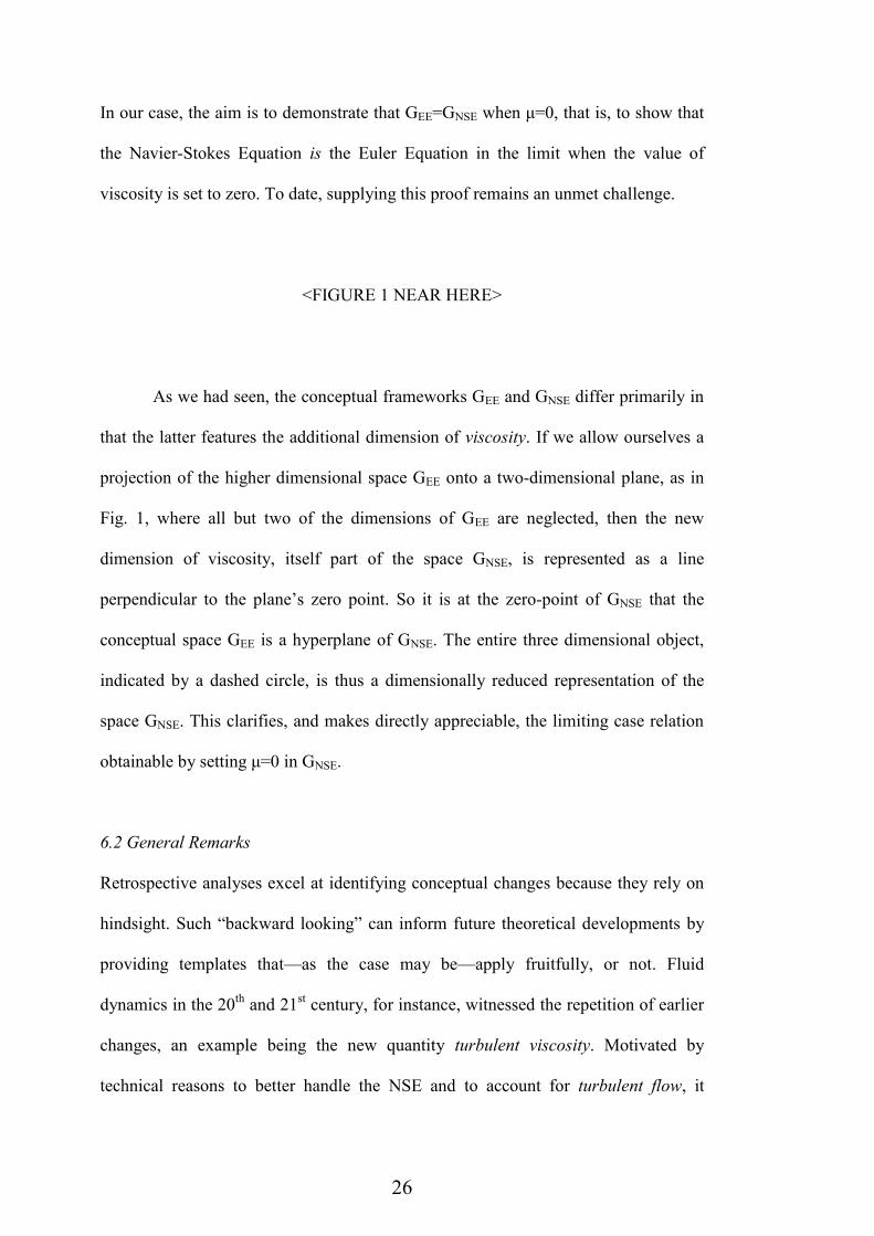
In our case, the aim is to demonstrate that GEE=GNSE when μ=0, that is, to show that

the Navier-Stokes Equation is the Euler Equation in the limit when the value of

viscosity is set to zero. To date, supplying this proof remains an unmet challenge.

<FIGURE 1 NEAR HERE>

As we had seen, the conceptual frameworks GEE and GNSE differ primarily in

that the latter features the additional dimension of viscosity. If we allow ourselves a

projection of the higher dimensional space GEE onto a two-dimensional plane, as in

Fig. 1, where all but two of the dimensions of GEE are neglected, then the new

dimension of viscosity, itself part of the space GNSE, is represented as a line

perpendicular to the plane’s zero point. So it is at the zero-point of GNSE that the

conceptual space GEE is a hyperplane of GNSE. The entire three dimensional object,

indicated by a dashed circle, is thus a dimensionally reduced representation of the

space GNSE. This clarifies, and makes directly appreciable, the limiting case relation

obtainable by setting μ=0 in GNSE.

6.2 General Remarks

Retrospective analyses excel at identifying conceptual changes because they rely on

hindsight. Such “backward looking” can inform future theoretical developments by

providing templates that—as the case may be—apply fruitfully, or not. Fluid

dynamics in the 20th and 21st century, for instance, witnessed the repetition of earlier

changes, an example being the new quantity turbulent viscosity. Motivated by

technical reasons to better handle the NSE and to account for turbulent flow, it

27

denotes the factor for a linear relationship between stress and mean flow, similar to

the material property viscosity, although stress is here restricted to turbulent stresses.

As we also saw, the specification of forces was linked to a change in

importance. But it is less clear vis-à-vis our analysis whether the increase in the

importance of forces had led to their specification or vice versa. Similarly, adding

laws such as Stokes’s theorem was seen to yield new dimensions such as pressure

that enriched the conceptual framework and linked it to thermodynamics via the gas

law. Generally, the motives for establishing such links will have to be provided by

science-historical scholarship. In a similar vein, ontological considerations were seen

to be less important when forces had been “lumped together.” Despite their distinct

ontological status, gravitational and electromagnetic forces, but also more fictitious

ones, came to be treated alike.17 Unlike long range ones, however, short range forces

are assumed to have direct molecular origin. Whatever might explain such

ontological non-commitments points beyond what we could provide in this article.

Generally, while a diachronic mode of dimensional analysis may be sufficient

in order to identify the conceptual changes that fluid dynamics underwent in the 19th

century, that mode is perhaps felt not to be necessary. We nevertheless take the

application of conceptual spaces to add value to extant modes of analyses that is

derived from its analytical distinctions. This contrasts favorably, in our opinion, with

17 With respect to their impact on a fluid volume, all are treated as long range

forces. Modern textbook treatments tend not not explain this change, but merely

restate it when declaring such forces to act equally on all matter contained in a

(given small) fluid volume, and to be proportional to the size of the volume

element and the density of the fluid (see Sect. 3.2).

28

extant uses of terms such as concept, dimension, domain, even scale, that tend to

make do without an explicit meta-framework defining such terms.

7. Conclusion

Using conceptual spaces as a meta-framework, this article identified changes to the

conceptual framework of 19th-century fluid dynamics which owe their salience to

being relevant explananda in the historical transition to the present day framework.

A concise summary was provided (Sect. 5). Compared to treating conceptual change

at the symbolic level of representation, the status of a theory’s axioms and laws has

here been demoted. Instead, the conceptual structures and their dynamics were traced

by analyzing the changes to the dimensions that constitute the conceptual framework,

and their inter-relations. The development from the Euler Equation to the Navier-

Stokes Equation was seen to involve all but one type of change, namely the deletion

of dimensions. The arguably most radical changes were the separation of forces, and

the introduction of velocity and viscosity to the spaces G and G*EE, respectively.

Moreover, a new spatial view on limiting case reduction was provided. As we have

argued, the transition from the Euler Equation to the Navier-Stokes Equation may be

viewed as an instance of normal science.

Acknowledgements

We consider this joint work, our names being listed in alphabetical order. We thank

Peter Gärdenfors and Ulrich Gähde, three anonymous reviewers, and the journal’s

editor, James W. McAllister, for comments that improved this manuscript. Graciana

Petersen acknowledges funding from the Environmental Wind Tunnel Laboratory,

University of Hamburg, and Frank Zenker from the Swedish Research Council (VR).

29

Appendix

Year Name Noted for

1738 D. Bernoulli Author of “Hydrodynamica,” known for Bernoulli’s law

1742 J. Bernoulli Author of “Hydraulica”

1743/44 D’Alembert Re-derived Bernoulli’s law

1752 L. Euler Found the Euler Equation using Newtonian mechanics

1781 J.L. Lagrange Worked on the Euler Equation, significantly changing his

view on which variables are relevant

1799 G.B. Venturi Conducted experiments on viscosity

1816 P.S. Girard Conducted experiments on flows in capillary tubes

1821

C.L.M.H.

Navier

Derived the Navier-Stokes Equation (NSE), i.e., the

viscosity extension of the Euler Equation

1821 H. Cauchy

Formulated a theory expressing elasticity in terms of

pressures acting on a surface, introducing tangential

pressures yielding the Cauchy stress tensor

1828 A. Cournot Criticized the NSE, naming it a “hypothesis that can solely

be verified by experiment”

1829 S.D. Poisson

Derived the NSE in a new way, inspired by Laplace’s

molecular physics, but mentioning neither Navier nor

Cauchy

1837

A.B. de Saint-

Venant Re-derived the NSE

1839 G. Hagen Conducted experiments on pipe flows

30

Table 1. Key Contributors to the 18th and 19th-Century Development of Fluid

Dynamics, based on Darrigol (2005) and Tokaty (1971)

1840 J.-L. Poiseulle Conducted experiments on pipe flows for the analysis of

blood circulation

1845 G.G. Stokes Derived the NSE in a new way, inspired by Cauchy and

Saint-Venan

1859 H. Helmholtz

Derived the NSE independently and worked on viscosity

(internal friction), seemingly unaware of the studies by

Poisson, Navier, Saint-Venan, and Stokes

31

References

Batchelor, G. (1970). An Introduction to Fluid Dynamics. Cambridge, UK:

Cambridge University Press.

Batterman, R. (2002). The Devil in the Details: Asymptotic Reasoning in

Explanation, Reduction, and Emergence. New York, N.Y.: Oxford University

Press.

Batterman, R. (2012). Intertheory Relations in Physics. In Zalta, E. N. (Ed.). The

Stanford Encyclopedia of Philosophy (Fall 2012 Edition).

http://plato.stanford.edu/archives/fall2012/entries/physics-interrelate/ (accessed

1 June 2014).

Chang, H. (2004). Inventing Temperature: Measurement and Scientific Progress.

New York, NY: Oxford University Press.

Darrigol, O. (2005). Worlds of Flow—A History of Hydrodynamics from Bernoulli to

Prandtl. Oxford, UK: Oxford University Press.

Einstein, A. (1905). Über die von der molekularkinetischen Theorie der Wärme

geforderte Bewegung von in ruhenden Flüssigkeiten suspendierten Teilchen.

Annalen der Physik, 17, 549–560.

Erdös, L. (2012). Lecture Notes on Quantum Brownian Motion. In Fröhlich, J.,

Salmhofer, M., Mastropietro, V., Roeck, W. de, & Cugliandolo, L.F. (Eds.),

Quantum Theory from Small to Large Scales (pp. 3–98). Ecole de Physique des

Houches, Session XCV, Oxford, UK: Oxford University Press.

French, S., & Kamminga, H. (Eds.) (1993). Correspondence, Invariance and

Heuristics: Essays in Honour of Heinz Post. Dordrecht: Kluwer Academic

Publishers.

Gärdenfors, P. (2000). Conceptual spaces: The geometry of thought. Cambridge,

MA: The MIT Press.

32

Gärdenfors, P., & Zenker, F. (2011). Using Conceptual Spaces to Model the

Dynamics of Empirical Theories. In: Olsson, E.J., and Enqvist, S. (eds).

Philosophy of Science Meets Belief Revision Theory (pp. 137 153). Berlin:

Springer.

Gärdenfors, P., & Zenker, F. (2013). Theory Change as Dimensional Change:

Conceptual Spaces applied to the dynamics of Empirical Theories. Synthese

190(6), 1039-1058.

Hartmann, S. (2002). On Correspondence: Essay Review of S. French and H.

Kamminga (Eds.) (1993). Studies in History and Philosophy of Modern Physics,

33, 79–94.

Hirschfelder, J. O.; Curtiss, C. F., & Bird, R. B. (1965). Molecular Theory of Gases

and Liquids. New York, NY: John Wiley and Sons.

Krantz, D. H., Luce, R. D, Suppes, P., & Tversky, A. (1971, 1989, 1990).

Foundations of Measurement, Volumes I-III. New York, NY: Academic Press.

Kuhn, T. (1970). The Structure of Scientific Revolutions (2nd edition). Chicago:

Chicago University Press.

Fefferman, C. L. (2014). Existence and Smoothness of the Navier-Stokes Equation.

Clay Mathematics Institute;

http://www.claymath.org/sites/default/files/navierstokes.pdf (accessed 25 May

2014).

Lakatos, I. (1978). The Methodology of Scientific Research Programs. Cambridge,

UK: Cambridge University Press.

Macagno, E. O. (1971). Historic-critical review of dimensional analysis. Journal of

the Franklin Institute, 292 (6), 391–402.

33

Maddox, W. T. (1992). Perceptual and decisional separability. In Ashby, G.F. (Ed.),

Multidimensional Models of Perception and Cognition (pp. 147–180). Hillsdale,

NJ: Lawrence Erlbaum.

Martins, R. de A. (1981). The origin of dimensional analysis. Journal of the Franklin

Institute, 311 (5), 331–337.

Melera, R. D. (1992). The concept of perceptual similarity: From psychophysics to

cognitive psychology. In Algom, d. (Ed.), Psychophysical Approaches to

Cognition (pp. 303–388). Amsterdam: Elsevier.

Petersen, G. (2013). Wind tunnel modelling of atmospheric boundary layer flow over

hills. Staats- und Universitätsbibliothek Hamburg/Max-Planck-Institute for

Meteorology. URN: urn:nbn:de:gbv:18-60540 (accessed 1 June 2014).

Post, H. (1971). Correspondence, Invariance, and Heuristics: In Praise of

Conservative Induction. Studies in History and Philosophy of Science, 2(3),

213–255.

Roche, J. (1998). The Mathematics of Measurement: A Critical History. London: The

Athlone Press.

Smoluchowski, M. (1906). Zur kinetischen Theorie der Brownschen

Molekularbewegung und der Suspensionen. Annalen der Physik, 21, 756–780.

Sneed, J. D. (1971). The Logical Structure of Mathematical Physics. Dordrecht:

Reidel.

Stevens, S. S. (1946). On the theory of scales of measurement. Science, 103, 677–

680.

Stegmüller, W. (1976). The Structuralist View of Theories. Berlin: Springer.

Suppes, P. (2002). Representation and Invariance of Scientific Structures. Stanford,

CA: CSLI Publications.

34

Tokaty, G. A. (1971). A History and Philosophy of Fluid Mechanics. New York, NY:

Dover Publications.

Zenker, F. & Gärdenfors, P. (2013). Modeling Diachronic Changes in Structuralism

and in Conceptual Spaces. Erkenntnis (online first).

http://link.springer.com/article/10.1007%2Fs10670-013-9582-9 (accessed 1 June

2014).

Zenker, F. & Gärdenfors, P. (2014). Communication, Rationality, and Conceptual

Changes in Scientific Theories. In Zenker, F. & Gärdenfors, P. (Eds.).

Applications of Geometric Knowledge Representation (Synthese Library Vol. X)

(pp. YY-ZZ). Dordrecht: Springer (forthcoming).

0

μ = viscosity

GEE

GNSE

(CAPTION FOR FIG 1 OF: Petersen and Zenker, From Euler to Navier-Stokes)

Fig. 1. Spatial view of limiting case reduction: The 2D plane GEE

is a hyperplane to the 3D space GNSE at the point μ=0 of GNSE.