UNIVERSITY OF NAIROBI, SCHOOL OF MATHEMATICS

A MASTERS OF SCIENCE IN APPLIED MATHEMATICS PROJECT

TOPIC

APPLICATION OF THE NAVIER-STOKES EQUATIONS IN THE LOCALISATION OF

ATHEROSCLEROSIS

BY

ANDREW MASIBAYI

I56/68715/2011

SUPERVISOR

PROF. CHANDRA BALI SINGH

Date: Sunday, July 28, 2013

© Nairobi – Kenya

Declaration

This project as presented in this report is my original work and has not been presented for any other

university award.

Signature:

Date:

ANDREW MASIBAYI

This project has been submitted as part of fulfillment for Masters of Science in Applied Mathematics of

the University of Nairobi with my approval as the supervisor.

Signature:

Date:

PROF. CHANDRA BALI SINGH

Acknowledgement

My sincere gratitude goes to my supervisor Prof. Singh Chandra Bali for his supportive supervision and

his patience for reading and correcting my work throughout the entire project time.

My great appreciation also goes to the director School of Mathematics and the entire Academic staff of

the School of Mathematics for the Knowledge they have imparted into me in the course of my studies in

this school, which have enabled me to come up with this project.

I would also like to thank all the MSc. Students in the school of Mathematics without whom; the last two

years wouldn’t have been so much fun and unforgettable. My special thanks go to Angwenyi David for all

the support he gave me in the course of the study.

I also appreciate my uncle, Edward Masibayi and my aunt Selina Namusasi for all the financial support

they gave me.

My most special thanks to my parents; John Masibayi and Beatrice Masibayi, who have been

continuously giving me support without them I would not have been able to go through the entire period.

Last but not least I thank almighty God whose generous strength, health and guidance enabled me

complete the project.

Contents

Acknowledgement ........................................................................................................................................ 1

Abstract .......................................................................................................................................................... i

1. Introduction ........................................................................................................................................... 1

1.1. Cardiovascular system .................................................................................................................. 1

1.2. Atherosclerosis .............................................................................................................................. 2

1.3. Description of the problem and approach ..................................................................................... 4

1.4. Objectives of the project ............................................................................................................... 4

2. Literature review ................................................................................................................................... 4

3. Mathematical model .............................................................................................................................. 5

3.1. Assumptions .................................................................................................................................. 5

2.2. Equations of motion in various coordinates .................................................................................. 5

2.2.1. Cartesian coordinates ............................................................................................................ 5

2.2.2. Equations of motion in cylindrical coordinates .................................................................... 8

2.2.3. Equations of motion in spherical coordinates ..................................................................... 17

2.3. Solution of the Navier-Stokes equations ..................................................................................... 20

2.3.1. Analytical solution of Navier Stokes equations .................................................................. 21

2.3.2. Numerical methods ............................................................................................................. 25

3. Bibliography ....................................................................................................................................... 55

4. Table of figures ................................................................................................................................... 56

Abstract

Localization of atherosclerosis plaque has been a great problem for many centuries. Many researchers

have done a lot of studies in blood flow with the motivations of understanding the localization of

atherosclerosis in arteries. This project presents a mathematical modeling of the arterial blood flow which

is derived from the Navier-Stokes equation and some assumptions. A system of non-linear partial

differential equations for blood flow is obtained. Finite element method (FEM) is then adopted to solve

the equations numerically. Apart from FEM, we will use the Galerkin stabilization method to solve the

problem of oscillations of solutions at high Reynolds numbers. We will also use the method of artificial

incompressibility and the Newton-Raphson method, to deal with the problems of incompressibility and

the problem of non-linear terms respectively. The results obtained will help in explaining the localization

of the atherosclerosis disease.

1

1. Introduction

In order to have a good understanding of this project, we need to have some basic knowledge of the

cardiovascular system, the atherosclerosis disease and also the wall shear stress.

1.1.Cardiovascular system

Cardiovascular system is a complex system in human body consisting of the heart, blood and blood

vessels. It’s a very vital component of human body, since it helps in supplying human body with nutrients

and oxygen and also helps in the removal of waste products; therefore without it human body cells will

die due to lack of nutrients and also due to accumulation of waste products. In order to have a good

understanding of cardiovascular system, we need to study how it works.

The circulatory system is divided into two parts; the low pressure pulmonary circulation, linking

circulation and gas exchange in the lungs and the high pressure systematic circulation, providing oxygen

and nutrients to body tissues.

Figure 1: Circulatory system (Gohil, 2002)

All arteries except Pulmonary artery carry oxygenated blood from the heart to body tissues. After the

blood has released oxygen to the tissues and taken up carbon dioxide, it’s carried back to the body

through veins, (Campbell, 1996, pp. 63-69). Therefore arteries carry and veins mainly carry oxygen and

carbon dioxide respectively. This explains why atherosclerosis plaques are found mostly in arteries. As

we will see later, this is because oxygen is involved in the formation of the disease and it’s mainly found

in arteries. In this project therefore we will only be concerned with arteries where the disease is most

likely to occur.

2

Arteries are subdivided into large and medium arteries, arterioles and capillaries. Therefore since blood is

not a homogenous fluid but is a suspension of particles in fluid called plasma, blood particles must be

taken into account in small arteries, the arterioles and capillaries since their size become comparable to

that of the vessel, hence blood is not homogenous in these arteries and have non standard behaviors, non-

Newtonian. On the other hand, in large vessels the size of the plasma suspensions is very small compared

to the radius of the vessels, hence fluid is homogeneous and shows standard behavior of a fluid,

Newtonian, (Quarterson, 2002). In this project we will consider blood to be Newtonian since we will

model blood flow through large vessels.

Carotid and coronary arteries supply blood to the brain and the heart respectively. These arteries are very

vital to human beings and interference with blood flow them can result into stroke and heart attack if the

carotid and coronary arteries are affected. These two diseases are among the leading diseases that causes

death, for instance, stroke is the third common cause of death (Chatzizis, 2008) and is also responsible for

5 million permanently disabled people per year worldwide, (Cheng, 2006).

1.2.Atherosclerosis

This is a disease in which cholesterol and calcium builds up in the inner lining of the arteries forming a

substance called plaque. Over time, the fat and calcium builds up narrows the artery and blocks blood

flow through it.

Figure 2: Atherosclerosis plaque

The origin of the atherosclerosis plaque, (Wake, 2005) is the excessive accumulation of low density lipo-

proteins (LDL) particles in the arterial wall. According to (Calves, 2010), the first step in the

atherosclerosis process is the accumulation of LDL cholesterol, in the intima, where part of it is oxidized

and becomes pathological. In order to remove it, circulating immune cells (e.g. monocytes) are recruited.

3

Ones in the intima, the monocytes differentiate to become macrophages that ingest by phagocytosis the

oxidized LDL. The ingestion of large amount of oxidized LDL transforms the fatty macrophages into

form cells, it’s these form cells which are responsible for the growth of sub-endothelial plaque which

eventually emerges in the artery lumen. Increase of macrophage concentration also leads to the

production of pro – inflammatory cytokines which contributes to recruitment of more macrophages.

Wall shear stress

Wall shear stress is the friction between the blood and the blood vessel walls. It depends on the velocity

and the viscosity of the blood. The wall shear stress, τ, in Cartesian coordinates is given by;

τ

and in cylindrical coordinates it’s given by; τ

is the coefficient of viscosity, and are small changes of velocity in – direction , small

changes of displacement in and radial directions respectively.

In no-slip boundary conditions wall shear stress is highest near the walls and decreases to zero as you

move towards the centre, while the velocity is highest at the centre and decreases as you move towards

the walls. This is shown below.

Figure 3: wall shear stress and velocity distribution

Low wall shear stress contributes to atherogenesis in the following way. Endothelial cells are highly

aligned and elongated when exposed to directional shear stress. In areas of low shear stress, endothelium

cells lose their alignment and organization leading to increased macromolecular permeability. This

allows cholesterol particles to enter the vessel wall and once oxidized they stimulate inflammatory

response and stimulate the migration and proliferation of smooth muscle cells into the growing lesion.

Since the amount of materials entering the region is greater than those leaving, the atherosclerosis plague

becomes larger.

4

1.3. Description of the problem and approach

Experimental results in vivo and in vitro have shown that atherosclerosis lesions develop in the vicinity of

branching arteries and strong curvature. In these areas, low wall shear stress has been established.

Measurement of wall shear in arteries has faced many challenges, which include difficulties in performing

these experiments in living organisms and also since the wall shear stress is very small, the measuring

instruments may not detect it, (Ritzen R. , 2012).

In this project to determine the wall shear stress distribution, we are going to derive the relationship

between wall shear stress distribution and velocity distribution and then use the distribution of velocity to

predict wall shear stress distribution.

To do this, we are going to solve the Navier-Stokes equations analytically and numerically and use the

solutions obtained in predicting the wall shear stress distribution. This will solve the problems

encountered in using the experimental methods.

1.4.Objectives of the project

The objectives of this project are;

- to convert the Navier – Stokes equations in Cartesian coordinates to different coordinate systems;

the cylindrical, and spherical coordinate

- to solve the Navier stokes equations analytically and using Numerical methods.

- to apply the solutions of the Navier-stokes obtained in explaining the localization of the

atherosclerosis.

2. Literature review

Several works have been done in this area. Some writers mainly concentrated on the solution of the Navier-

Stokes which they did successfully. For instance, (Jiajan, 2010), was able to solve the non-linear two

dimension Navier-Stokes equations. He successfully dealt with the non – linear problem by using the

Newton – Raphson method which reduced algebraic equations to linear. In his work, the problem of

instability was solved by using Galerkin stabilization method. And finally he dealt with the problem of

incompressibility condition by adding an artificial term to the continuity equation. Although he successfully

solved the Navier – Stokes equations, he did not apply the solutions obtained to blood flow problems.

Another person who did research in this area is (Kazakidi, 2008). He was able to give a good mathematical

back-ground of atherosclerosis and its relationship with wall shear stress. He then solved the equations by

finite element method.

Other researchers like (Gohil, 2002), used Cosmol Multiphysics software to simulate the distribution of

wall shear stress at bifurcation points.

5

In this project, we have extended the mathematical background given by (Kazakidi, 2008) using the work

done by (Jiajan, 2010). Furthermore in this project we derive the relationship between wall shear stress and

velocity, and then predict the wall shear stress distribution by only considering the velocity distribution.

3. Mathematical model

In this section we are going to come up with equations that describe blood flow in blood vessels, the

Navier Stokes, and continuity equations. We will first write the equations in different coordinates, and

then solve them both analytically and by numerical methods. Since blood is very complex, for instance,

the blood is non-Newtonian, the flow is turbulent and also it is unsteady, we will first simplify the

problem by coming up with several assumptions.

3.1.Assumptions

The flow in arteries is very complex, and it may be very difficult to come up with the equation to describe

it. y. To simplify the problem we make some assumptions;

1. The blood is Newtonian; it obeys Newton’s laws of motion. This assumption is very important to

this project because it will enable us to use the Navier-Stokes equations. This assumption is

justified since we are going to base our model on large vessels where blood behaves as if it is

Newtonian

2. The blood is incompressible. With this assumption, the balance of mass and the balance of

momentum turn into Navier Stokes Equation as the governing equation of motion.

2.2.Equations of motion in various coordinates

In this section, we are going to look at the equations of motion in Cartesian, cylindrical and spherical

coordinates.

2.2.1. Cartesian coordinates

In Cartesian coordinates, the Navier-Stokes and the continuity equations are given by;

(a) Continuity equation

The general form of equation of conservation of mass is given by

( ) ( ) ( )0

u v w

t x y z

(1)

In equation above, and are velocities in and - directions and is the density.

The above equation is valid for steady and unsteady, compressible and incompressible fluid. In vector

form, equation can be written in vector form as;

t

= 0 (2)

6

Equation (1) is the first form of continuity equation

Here, x y z

i j k and u v w i j k

The continuity equation can also be written in another form, we use product rule on the divergent term in

equation (2) to get,

(3)

In equation (3) above, the terms,

can be replaced by the material derivative,

, therefore

equation (2) will become,

(4)

Equation four is the second form of continuity equation

There are two special cases for the continuity equation (2)

1. For Steady flow, the equation does not depend on time, therefore equations (1) and (2) becomes

( ) ( ) ( )0

u v w

x y z

(5)

Or in vector form

. = 0 (6)

this follows since by definition, is not a function of time for steady flow, but could be a function

of position.

2. For incompressible fluids the density, is constant throughout the flow field so that the equations

(1) and (2) become;

∇∙ 0 (7)

Or

0u v w

x y z

(8)

The above equation is a special form of equation (5) when density is not a function of position and it

applies to both steady and unsteady flow of incompressible fluids; this is the equation we will use in this

project since we will assume that blood is incompressible as stated in the assumptions.

7

(b) The Navier stokes equations

Navier-Stokes equations are the equations of conservation of linear momentum. The general form of the

equations for incompressible flow of Newtonian (constant viscosity) fluid is given by;

∇

∇ (9)

is kinetic viscosity (constant) and is given by

, is density (constant), is pressure and is the

gravitational force.

In the equation (9) above,

-

– Acceleration term

- – is the advection term; the force exerted on the particles of the fluid by other particles of

the fluid surrounding it

- ∇ – velocity diffusion terms; describes how the fluid motion is damped, highly viscous fluid

e.g. honey stick together while low viscous fluid flow freely, e.g. air

- - pressure term, fluids flow in the direction of largest change in pressure

From equation (2), ∇ x y z

i j k and u v w i j k . Replacing this in equation (9) we

obtain

∇

(10)

In equation (10) the laplacian is given by

∇

Replacing the laplacian above in equation (10), we obtain

(11)

Collecting coefficients of, together, this leads to equations in directions respectively

as follows;

(12)

8

The above three equations are the Navier-Stokes equations in and components. In this project we

will neglect the body forces. Therefore dropping the body forces and rearranging the equations we obtain;

-component

2 2 2

2 2 2x

u u u u p u u uu v w g

t x y z x x y z

(13)

-component

2 2 2

2 2 2y

v v v v p v v vu v w g

t x y z y x y z

(14)

-component

2 2 2

2 2 2z

w w w w p w w wu v w g

t x y z z x y z

(15)

Here, is the coefficient of viscosity, is the density of the fluid and g is the gravitational force

2.2.2. Equations of motion in cylindrical coordinates

In cylindrical coordinates, the coordinates is the radial distance from the axis, is the angle measured

from a line parallel to the - axis, is the coordinates along the - axis. The velocity components are the

radial velocity the tangential velocity and the axial velocity . Thus the velocity at some arbitrary

point can be expressed as

r zu u u r θ z

q e e e (16)

Figure 4: Shape of an artery

Cartesian coordinates can be expressed into cylindrical coordinates using the relations,

cos , sin , and x r y r z z (17)

The above relations implies that

( , )

( , )

x x r

y y r

z z

(18)

I.e. Cartesian coordinates can be expressed in terms of cylindrical coordinates, also

9

1 2 2tan , , y

r x y z zx

(19)

This relations also implies that

( , ), ( , ), x y r r x y z z (20)

Therefore equations (20) and (18) show the relationship between Cartesian coordinates and cylindrical

coordinates. In general form, the relationship between Cartesian coordinates and any other coordinate

system can be represented by,

1 2 3 1 1

1 2 3 2 2

1 2 3 3 3

( , , ) ( , , )

( , , ) ( , , )

( , , ) ( , , )

x x u u u u u x y z

y y u u u u u x y z

z z u u u u u x y z

In the above equation, 1 2 3, , u u u are the curvilinear coordinates, they can be cylindrical coordinates or

spherical coordinates. In cylindrical coordinates;

1 2 3, and ur zu u r u u u z (21)

To convert Cartesian coordinates to cylindrical coordinates, we first convert them into curvilinear

coordinates before to cylindrical coordinates.

In this section we will transform the continuity and momentum equations from Cartesian to cylindrical

coordinates. We will start by converting the continuity equation, and then followed by the momentum

equations.

(a) Continuity equation

The continuity equation in vector form as shown in (7) is given by;

∇∙ 0

In order to understand how to convert the equation in curvilinear coordinates, we first need to first know

several parameters which we are going to use.

Unit vectors (in curvilinear coordinates)

In curvilinear coordinates and the unit vectors, , and are given by

i

i

u

u

i

re

r

1

i ih u

r (22)

Where,

r is a position vector of any point in Cartesian coordinate system and is given by;

x y z r i j k (23)

10

iu r Is a vector in the direction of the tangent to the iu - curve. In cylindrical coordinates, the unit

vectors , and are given as , and .

Scale factors

We will take the curvilinear coordinates and to be orthogonal. From equation (22), the scale

factors are where and are given by;

i

i

hu

r (24)

In equation (24) above,

x y z r i j k (25)

Replacing equation (25) into equation (24) we obtain the equation,

i

i i i i

r x y zh

u u u u

i j k (26)

From equation (26) above, we get,

2

2 2 2

i

i i i i i i i i

i i i

r r x y z x y zh

u u u u u u u u

x y z

u u u

i j k i j k

(27)

Replacing equation (17) into (27), we obtain

2 2 2

2 cos sin

1, 2 and 3

i

i i i

h r r zu u u

i

(28)

In cylindrical coordinates the scale factors; , and and the coordinates , and are given by;

1 2 3

1 2 3

and h

, ,

r z

r z

h h h h h

u u r u u u u z

(29)

Now replacing (29) into (28) above we get

2 2 2 2 2 2

2

2 2

( cos ) ( sin )

cos sin 1

r

x y zh r r z

r r r r r r

(30)

11

2 2 2 2 2 2

2

2 2 2 2 2

( cos ) ( sin )

cos sin

x y zh r r z

r r r

(31)

2 2 2 2 2 2

2 ( cos ) ( sin ) 1z

x y zh r r z

z z z z z z

(32)

From the equations; (30), (31) and (32), the scale factors in cylindrical coordinates are;

1, , 1r zh h r h (33)

Now after the above explanations, we now express the continuity equation ∇∙ 0 in cylindrical

coordinates. We first express the divergence, ∇∙ in curvilinear coordinates. Before we do this, we first

find the value of Del operator, ∇ in curvilinear coordinates. To do this, we first find the value of ,

where is any scalar function. In curvilinear coordinates, it will be written as

1 1 2 2 3 3f f f e e e (34)

1 2 3e e e , are unit vectors along 1 2 3, , u u u curves.

Let be a position vector of a point in Cartesian coordinates. Then from (25) is given by

x y z r i j k

Using the relations (17) the equation above becomes

cos sinr r z r i j k (35)

We need to express in two different ways and compare the coefficients of and to

obtain the values of, , , and in equation (34).

In the first expression,

d dx dy dz dx dy dzx y z x y z

dr

i j k i j k (36)

Then using equation

1 2 3( , , )u u ur r

1 2 3

1 2 2

d du du duu u u

r r rr (37)

From (22), equation (37) can be written as

12

1 1 2 2 3 3d h du h du h du 1 2 3r e e e (38)

We therefore obtain

1 2 3 1 1 2 2 3 3

1 1 1 2 2 2 3 3 3

. .

d dr f f f h du h du h du

f h du f h du h f du

1 2 3 1 2 3e e e e e e (39)

d can also be expressed as,

1 2 3

1 2 2

d du du duu u u

(40)

Comparing equations (39) and equations (40), get the following,

1 2 3

1 1 2 2 3 3

1 1 1 f f f

h u h u h u

(41)

Replacing (41) in (34) we obtain,

1 1 2 2 3 3

1 1 1

h u h u h u

1 2 3e e e (42)

Therefore, from equation (42)

1 1 2 2 3 3

1 1 1

h u h u h u

1 2 3e e e (43)

In cylindrical coordinates, equation (43) can be written as

1

r r z

r θ ze e e (44)

We will then proceed to find the value of in curvilinear coordinates. In curvilinear coordinates, we

will take to be equal to

1 2 3 1 2 3( ) ( ) ( ) ( )u u u u u u 1 2 3 1 2 3q e e e e e e (45)

From, equation (42) above,

1 1 1

1 3

1 1 2 2 3 3 1

1 1 1u u uu

h u h u h u h

1

1 2

ee e e (46)

32 2

2

1 1 2 2 3 3 2

1 1 1 uu uu

h u h u h u h

2

1 2 3

ee e e (47)

3 3 3

3

1 1 2 2 3 3 3

1 1 1u u uu

h u h u h u h

3

1 2 3

ee e e (48)

13

We then deal with each term on the right hand-side of equation (45), but first we derive certain relations.

From equations (46), (47) and (48), we obtain;

2 3 2 3 2 3

2 3 2 3

u u h h u uh h h h

2 31

1

e eee (49)

1 3 1 3 1 3

1 3 1 3

u u h h u uh h h h

1 32

2

e ×eee (50)

1 2 1 2 1 2

1 2 1 2

u u h h u uh h h h

3 1 2

3

e e ×ee (51)

We will then express all the terms on the left hand-side in equation (45) in curvilinear coordinates, we

will begin with the term, ( )u 1e

1 2 3 1 2 3

2 3 1 2 3 2 3 2 3 1

( )

.

u h h u u u

h h u u u u u h h u

1e (52)

But in equation (52) above,

2 3 3 2 2 3 0u u u u u u

Hence,

1 2 3 2 3 1( ) .u u u h h u 1e (53)

From equations, (47 – 49), equation (53) becomes

1 2 3 1

2 3

( ) .u h h uh h

1

1

ee (54)

Using equation (42), we can express 2 3 1( )h h u in the above equation as

2 3 1 2 3 1 2 3 1

2 3 1

1 1 2 2 3 3

1 1 1h h u h h u h h uh h u

h u h u h u

1 2 3e e e (55)

Now replacing equation (55) into (54) we obtain

1 2 3 1 2 3 1 2 3 1

2 3 1 1 2 2 3 3

1 1 1( )u h h u h h u h h u

h h h u h u h u

1

1 1 2 3

ee e e e (56)

Simplifying equation (56), we obtain,

1 2 3 1

1 2 3 1

1( )u h h u

h h h u

1e (57)

In a similar way the remaining two terms in equation (42) can be found to be

14

2 1 3 2

1 2 3 2

1( )u h h u

h h h u

2e (58)

3 1 2 3

1 2 3 3

1( )u h h u

h h h u

3e (59)

Replacing equations (57 – 59) in (45) we obtain

2 3 1 1 3 1 1 2 1

1 2 3 1 1 2 3 2 1 2 3 3

1 1 1h h u h h u h h u

h h h u h h h u h h h u

q (60)

Using equations (33) we can now express equation (60) in cylindrical coordinates as

1 1r zru u u

r r r z

q (61)

(b) Momentum equation

The momentum equation in vector form as shown in equation (9)

2.q

p pt

q q g q

We want to express the above equation in cylindrical coordinates. Since we have already calculated the

value of the grad, we only need to find the value of the Laplacian,2 . To do this, we first find the

value of ∇ , where is any scalar function and then and then finally find the laplacian.

2 f f (62)

We then let

, where (63)

From equation (42),

2

1 1 2 2 3 3

f fF f

h u h u h u

31ee e

(64)

Comparing coefficients of and 1 2 3e , e e , in equations (63), (64), we obtain;

1 2 3

1 1 2 2 3 3

1 1 1, ,

f f fF F F

h u h u h u

(65)

From equation (60), equation (62) can be written as,

2

1 2 3

2 3 1 1 3 2 1 2 3

1 2 3 1 2 3

( ) ( )

1 =

f f F F F

h h F h h F h h Fh h h u u u

1 2 3F e e e

(66)

15

Equation (66) can be simplified to

2 2 3 1 3 1 2

1 2 3 1 1 1 2 2 2 3 3 3

1 h h h h h hf f ff

h h h u h u u h u u h u

(67)

Hence the laplacian in curvilinear coordinates is given by;

2 2 3 1 3 1 2

1 2 3 1 1 1 2 2 2 3 3 3

1 h h h h h h

h h h u h u u h u u h u

(68)

In cylindrical coordinates, equation (68) becomes

2 22

2 2 2

1 1r

r r r r z

(69)

The gravitational force, in cylindrical coordinates can be written as,

r zg g g r θ zg e e e (70)

Substituting, 2, and g from equations; (42), (69) and (70) respectively, in equation (60),

2. p pt

qq q g q

We obtain;

2 2

2 2 2

1.

1 1 1

r z r z r z

r z r z

u u u u u u u u ut r r z

p p g g g r u u ur r z r r r r r z

r θ z r θ z r θ z r θ z

r θ z r θ z r θ z

e e e e e e e e e e e e

e e e e e e e e e

(71)

On simplifying equation (71), we obtain

2 2

2 2 2

1

1

1 1

r z r z r z

r z

r

u u u u u u u u ut t t r r z

p p ppg pg pg

r r z

r u ur r r r z

r θ z r θ z r θ z

r θ z r θ z

r

e e e e e e e e e

e e e e e e

e zu θ ze e

(72)

16

1 1

1 1

1

r z r z r r z

r z z r z

u u u u u u u u u u ut t t r r z r r z

p p pu u u u pg pg pg

r r z r r z

rr r r

r θ z r θ z r r θ z θ

r θ z z r θ z r θ z

e e e e e e e e e e e

e e e e e e e e e e

2 2 2 2 2 2

2 2 2 2 2 2 2 2 2

1 1 1 1 1r zu r u r u

r r r r r rr z r z r z

r θ ze e e

(73)

Now collecting terms that containre , we obtain;

2 2

2 2 2

1 1r r z r r r

pu u u u u pg r u

t r z r r r r r z

(74)

While those that contain θe , are

2 2

2 2 2

1 1r z

pu u u u u pg r u

t r z r r r r z

(75)

And finally those containing ze are

2 2

2 2 2

1 1z r z z z z

pu u u u u pg r u

t r z z r r r r z

(76)

Therefore, equations; (74), (75) and (76) are the Navier – Stokes equation in cylindrical coordinates. On

simplifying the three equations we obtain

r-component

2

2 2

2 2 2 2 2

1 1 1

r r r rr z

r r r rr

u uu u u uu u

t r r r z

uu u u upq r

r r r r r r r z

(77)

- component

2 2

2 2 2 2 2

1 1 1 2

r rr z

u u u u u u uu u

t r r r z

u u u u upq r

r r r r r r r z

(78)

z- component

17

2 2

2 2 2

1 1

z z z rr z

z z zz

uu u u uu u

t r r z

u u upq r

z r r r r z

(79)

2.2.3. Equations of motion in spherical coordinates

Finally, we shall convert the equations of motion in spherical coordinates. In this section however we will

not convert the equations of motion in curvilinear coordinates since we have already done this in the

previous section. We will simply use what we have already derived.

The coordinates of a point P in spherical coordinates is given by the ordered pair, and .

- is the distance from the origin to the point P

- is the angle between the axis and the line from the origin to the point P

- is the angle between the axis and the line from the origin to the point P

The relationship between the cylindrical coordinates and the spherical coordinates is given by;

sin cos , sin sin , cosx r y r z r (80)

Scale factors

In spherical coordinates, the scale factors are, , and rh h h as shown in equation (26) are given by;

2 2 2

2

i

i i i

x y zh

u u u

(81)

Where , and i r

2 2 2

2

r

r r r

x y zh

u u u

(82)

2 2 2

2

2 2 2 2 2 2 2 2 2

sin cos sin sin cos

sin cos sin sin cos sin cos sin cos 1

rh r r rr r r

(83)

Similarly can be given by

2 2 2

2 x y zh

u u u

(84)

18

2 2 2

2

2 2 2 2 2 2 2 2 2 2 2 2

sin cos sin sin cos

sin sin sin cos sin sin cos sin

h r r ru u u

r r r r

(85)

Similarly, can be expressed as

2 2 2

2 x y zh

u u u

(86)

2 2 2

2

2 2 2 2 2 2 2 2 2 2 2 2 2 2

2 2 2 2

sin cos sin sin cos

cos cos cos sin sin cos cos sin sin

cos sin

hu u u

r r r r r

r r

(87)

Therefore the scale factors in spherical coordinates are given by

2 1, sin , and rh h r h r (88)

In spherical coordinates, the velocity vector is given by,

r rq u e u e u e (89)

We will then express in spherical coordinates, the continuity equations and the momentum equation

(a) Continuity equation

We will express the continuity equation in equation (7) = 0 in curvilinear coordinates. From

equation (60), we have;

2 3 1 1 3 1 1 2 1

1 2 3 1 1 2 3 2 1 2 3 3

1 1 1h h u h h u h h u

h h h u h h h u h h h u

q

In spherical coordinates,

1 2 3, and are , and ru u u u u u (90)

Using equations (93) and (95), we obtain;

2

2 2 2

2

2 2 2

1 1 1sin sin

sin sin sin

1 1 1sin

sin sin

r

r

r u ru r urr r r

r u ru r urr r r

q

(91)

19

(b) Navier-Stokes equations

To express in spherical coordinates, the Navier-Stokes equation (60);

2. pt

qq q g q

We first express the grad, laplacian, velocity and gravity in spherical coordinates.

In curvilinear coordinates, the laplacian from equation (67) is given by

2 2 3 1 3 1 2

1 2 3 1 1 1 2 2 2 3 3 3

1 h h h h h h

h h h u h u u h u u h u

Replacing equation (92) and (94) into the above equation we obtain

2 2

2

1 1sin sin

sinsin r rr

(92)

We can also express g as

rg g g r θg e e e (93)

From equation (43), in curvilinear coordinates, grad is given by;

1 1 2 2 3 3

1 1 1

h u h u h u

1 2 3e e e

In spherical coordinates the above equation is written as;

1 1

sinr r r

r θe e e (94)

And finally we have;

ru u u r θq e e e (95)

Now replacing equations, (92), (94) and (95) into equation (60) we obtain,

2

2

1 1.

sin

1 1

sin

1 1sin sin

sinsin

r r r

r

u u u u u u u u ut r r

p g g gr r r

rrr

r θ r θ r θ r θ

r θ r θ

e e e e e e e e e e e e

e e e e e e

ru u u

r θe e e

(96)

Expanding equation (96) we obtain

20

2

2

sin

1 1

sin

1 1sin sin

sinsin

r r r

r

uuu u u u u u u

t t t r r

p p pg g g

r r r

rrr

r θ r θ r θ j

r θ r θ

e e e e e e e e e

e e e e e e

ru u u

r θe e e

(97)

We then write equation (97) in component form, we first collect all the terms withre ;

2

2

sin

1 1sin sin

sinsin

r r r r

r

uu pu u u g

t r r r r

r ur rr

(98)

Similarly terms containing θe are,

2

2

1

sin sin

1 1 sin sin

sinsin

r

uu pu e u u g

t r r r

r urr

(99)

And finally the terms containing e

2

2

1

sin

1 1sin sin

sinsin

r

uu pu u u g

t r r r

r urr

(100)

Equations; (98), (99) and (100) are the momentum equations in spherical coordinates.

2.3.Solution of the Navier-Stokes equations

These equations are very complex and it is very difficult to solve them analytically. This is because of

their non-linear terms arising from the convective acceleration terms. However there are a few special

cases for which the convective acceleration vanishes because of the nature of the geometry of the flow

system, in such cases exact solutions are possible. In this project, we are going to first solve the equations

analytically; this will help us have an idea of the distribution of velocity and wall shear stress and finally

we solve using numerical methods.

21

2.3.1. Analytical solution of Navier Stokes equations

Analytical solution is obtained when governing Boundary Value Problem is integrated using the methods

of classical differential equations. Full Navier – Stokes equations have no known general analytical

solution due to its complexity. In order to solve the equations analytically we simplify them by making

several assumptions about the fluid, the flow or the geometry of the problem. The assumptions are; we

assume the flow is laminar, steady, incompressible and parallel between plates. By making these

assumptions it’s possible to obtain the analytical solutions. The continuity equation and the momentum

equation for steady incompressible flow as shown in equations (1) (13), (14) and (15) are given by;

0u v

x y

(101)

2 2

2 2

1u u p u uu v

x y x x y

(102)

2 2

2 2

1v v p v vu v

x y y x y

(103)

Since the flow is constrained by flat parallel walls of the channel, no component of the velocity in y and z

directions; this implies that 0v w . Also the gradient in and v w are zero, i.e.

2 2 2 2 2 2

2 2 2 2 2 20 also; 0

v w v w w v w v w v w v

y y z z x x x y y z z x

(104)

Therefore the equations above become;

2

20 this implies that 0

u u

x x

(105)

2 2

2 2

dp d u d u

dx dy dx (106)

Using equation (106), equation (107) becomes;

2

2

dp d u

dx dy (107)

The above equation implies that u is not a function of x alone therefore, dp

dx is constant .On integrating

it twice we obtain the results;

22

2

2

1

1

d u dpdy dy

dxdy

du dpy A

dy dx

, where A is a constant

On integrating again we obtain

21( )

2

dpu y y Ay B

dx , B is another constant (108)

In the next step now we calculate the values of the constants of integration, A and B. To do this, we apply

the no – slip boundary conditions at the walls. The boundaries conditions are;

At , 0 and also at , 0y h u y h u (109)

Applying the boundary conditions in equations (110) to equation (109), we obtain;

2 21 1 1 10 , and 0

2 2

dp dph Ah B h Ah B

dx dx . Solving these equations simultaneously, we

obtain; A=0 and

21

2

h dpB

dx . Substituting for A and B in equation (110), we get,

22 221 1 1 1

( ) 12 2 2

dp h dp h dp yu y y

dx dx dx h

(110)

Equation (111) can be used to calculate the velocity distribution in a pipe, in radial direction

Wall shear stress can be calculated from equation (111) by using the relation;

du

dy (111)

Substituting equation (111) into (112), we obtain;

dPy

dx (112)

From equation (113) above we get that wall shear stress is zero at the centre where y= 0 and maximum on

the walls, where y = h.

To have a clear picture on how velocity and wall shear stress is distributed in a straight pipe, we plot the

equations (111) and (113) respectively.

23

Plot of velocity distribution in a straight pipe

Equation of velocity in a straight pipe is given by (111);

221( ) 1

2

h dp yu y

dx h

, in this equation we will take the radius of the pipe, h = 0.5 and the value

of

21

2

h dp

dx= 1, then the equation becomes;

2

( ) 10.5

yu y

(113)

We then plot the equation (111) using MATLAB

Figure 5: Velocity distribution in a straight pipe

To calculate wall shear stress, we replace equation (114) to equation (113) to obtain;

4du

ydy

(114)

The plotting, we obtain the graph below,

Figure 6: Stress distribution in a straight pipe

24

Velocity and wall shear stress distribution at bifurcation point.

From the above explanations, it’s clear that, velocity is symmetric about the axis. However for flows at

bifurcation points, this is not the case. The velocity curve tends to lean on one side more than the other, as

shown below.

Figure 7: Velocity distribution at bifurcation point

From the figure above, as the fast moving flow arrives at the flow divider of the bifurcation, it is forced to

follow one of the branches. Due to its high inertia, acting pressure gradient cannot displace it immediately

into axial directions of the daughter branches and hence the flow moves next to the inner walls of the

bifurcation (Kazakidi, 2008).

To explain this curve equation (112) can be modified as follows;

221( ) 1 where,

2

h dp y yu y k h

dx K h

(115)

Taking;

2

2

10.5, k=0.8 and 1, we will obtain,

2

10u(y)=1+ (2 )

8

h dph

dx

y y

Plotting the equation above we obtain the graph given below

Figure 8: Velocity distribution at branch point

25

To get the wall shear stress distribution we differentiate the equation for velocity to get;

108

8

duy

dy (116)

On plotting the above curve we obtain;

Figure 9: Stress distribution at branch point

The above equation (117) gives the wall shear stress on the outer wall. Clearly the wall shear stress in the

equation (117) is less than that in equation (115). Hence wall shear stress is lower on the inner side of the

wall at bifurcation point than on the straight tube.

2.3.2. Numerical methods

There are various numerical methods which can be used to solve them, finite element method, finite

volume method, finite difference method and Lattice Boltzmann Method. All these methods can be used

to solve the equations. However in this project, we are going to concentrate on only one method, the finite

element method, since it’s simple and able to solve complex geometries compared to other methods.

Furthermore by this method we are able to include boundary conditions in the formulations. Before we

look at how to solve the Navier-Stokes equations using the finite element method, we are going to have a

brief introduction to what is FEM using a simple example.

Finite Element Method

Finite element method is a numerical procedure for solving the differential equations in of physics and

engineering (J.Segerlind, 1976). In this method, the solution domain is divided into simply shaped regions

or elements, then an approximate solution of the partial differential equation can be developed for each of

26

these elements and finally, the total solution is then generated by linking together the individual solutions.

To explain how this method works, we are going to consider one dimension and two dimension case.

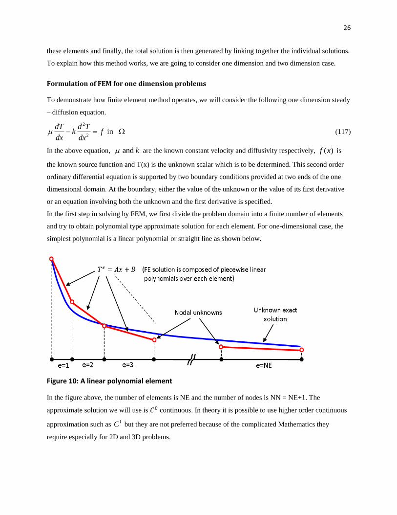
Formulation of FEM for one dimension problems

To demonstrate how finite element method operates, we will consider the following one dimension steady

– diffusion equation.

2

2 in

dT d Tk f

dx dx (117)

In the above equation, and k are the known constant velocity and diffusivity respectively, ( )f x is

the known source function and T(x) is the unknown scalar which is to be determined. This second order

ordinary differential equation is supported by two boundary conditions provided at two ends of the one

dimensional domain. At the boundary, either the value of the unknown or the value of its first derivative

or an equation involving both the unknown and the first derivative is specified.

In the first step in solving by FEM, we first divide the problem domain into a finite number of elements

and try to obtain polynomial type approximate solution for each element. For one-dimensional case, the

simplest polynomial is a linear polynomial or straight line as shown below.

Figure 10: A linear polynomial element

In the figure above, the number of elements is NE and the number of nodes is NN = NE+1. The

approximate solution we will use is continuous. In theory it is possible to use higher order continuous

approximation such as 1C but they are not preferred because of the complicated Mathematics they

require especially for 2D and 3D problems.

27

The method of weighted residual and the weak form of the equation

The diffusion equation (123) together with boundary conditions is known as the strong form of the

problem. FEM is a weighted residual type numerical method and it makes use of the weak form of the

ODE. In order to obtain the weak for, we first obtain the residual; the residual of the DE is obtained by

collecting all the terms on one side as follows;

2

2( )

dT d TR x k f

dx dx (118)

It’s important to note that for exact solution T(x), R(x) = 0. But for an approximate solution, the residual

will not vanish. This implies that the smaller the residual the closer the approximate solution to the exact

solution. The method of weighted residual tries to minimize the residual in a weighted integral sense as

follows;

( ) ( ) , where, R( ) is the residual and w(x) is weght functionw x R x dx x (119)

Substituting the residual into this equation we obtain,

2

20

dT d Twu wk wf dx

dx dx

(120)

Since we have NN unknowns, we will choose as many functions to obtain NN equations. Since we are

using 0C continuous solution in the above weighted residual statement, the second order derivative that

appears in the diffusion term in equation (121) cannot be evaluated properly. In order to be able to work

with a 0C continuous approximation solution, we need to lower the differentiation requirement of the

unknown in the weighted residual statement. This is done by applying integration by parts to the second

term (diffusive term) of the equation (121). But before we do this we state the following theorem;

Theorem: Fundamental theorem of calculus, x

udx un d

y

where nx is a unit a unit outward

normal to the boundary, of .

Using the above theorem we write the diffusion term as

2 2

2 2, x

d T d dT dw dT d T dw dT dTw wk k w k wk n d

dx dx dx dx dx dx dxdx dx

(121)

28

The last term in the second part of equation above is called a boundary integral. This term is evaluated at

the boundaries of the problem domain , where nx is the x – component of the unit outward normal to

the boundary.

It’s now important to note that the integration by parts have lowered the differential order of the unknown

T from 2 to 1 and increased the differential order of the of the weight function from 0 to 1. Integration by

parts is not applied to the advection term, because it only contains a first order derivative of T.

On substituting the diffusion term back into the weighted equation (121), we obtain;

+ x

dT dw dT dTwu k dx wfdx wk n d

dx dx dx dx

(122)

We note that, the terms on the left hand side of the above equation now includes only first order

derivatives of the unknown. This is called the weak form of the problem due to this lower differentiability

requirement compared to the original weighted residual statement. The weak forms allow us to work with

0C continuous approximate solutions.

Primary and secondary variables and boundary conditions

In finite element method formulation, the boundary term on the RHS of equation (123) is very important.

This is because it can be used identify the primary and secondary variables of a problem. To do this, we

separate the boundary term into two parts; the first part containing the weight function and possibly its

derivatives and the second part contains the dependent variable and possibly its derivatives. In our case,

the first part includes only w. The dependent variable of the problem T, expressed in the same form as

this first part of the boundary term called the primary variable, for this problem, Primary variable is T.

Part two includes, x

dTwk n

dx, which is the secondary variable of the problem. Secondary variables

always have important physical meaning such as the amount of heat flux that passes through the boundary

in heat transfer. If secondary variable is provided at a boundary is known as a natural or Neumann

boundary condition and if primary variable is provided at a boundary the problem is known as essential

(Dirichlet) boundary condition. If both Secondary and Primary variables are provided, then the problem is

called mixed boundary condition.

Essential BC (EBC): T = T0

Natural BC (NBC): 0x

dTk n q

dx

Mixed BC (MBC): x

dTk n T

dx

29

Constructing approximate solution

The 0C approximate solution is given by;

1

( ) ( )NN

app j j

j

T x T S x

(123)

Where appT is the approximate solution, NN is the number of nodes in the FE mesh,

jT ’s are the nodal

unknown values that we are going to calculate at the end of the finite element solution and jS ’s are the

shape functions that are used to construct the approximate solution.

Mesh function have compact support in that, they are non-zero only over the element which touch the

node with which they are associated with, everywhere else, they are equal to zero.

We now substitute the approximate solution given in (124) into (123) to obtain

1 1

+ ( )NN NN

j j

j j

j j

dS dSdwwu T k T dx wfdx wk SV d

dx dx dx

(124)

Since we have NN unknowns, we need to have NN equations; therefore we need to select the weight

functions NN times. In using Galerkin finite element method, the weight functions are selected are same

as the shape functions, i.e.

( ) ( )iw x s x

Using the above substitution equation (130) becomes;

1 1

+ ( )NN NN

j ji

i j j i i

j j

dS dSdSS u T k T dx S fdx S SV d

dx dx dx

(125)

Putting the summation sign outside, we obtain,

1

+ ( ) i = 1,2,3,....NN

ji i

i j i i

j

dSdS dSS u k dx T S fdx S SV d

dx dx dx

(126)

To further simplify the equation we can use the following compact matrix notation,

[K]{T} = {F} + {B}

Which is known as the global equation system, {T} is the vector of nodal unknowns with NN entries, [K]

is the global square stiffness matrix of the size NN x NN with entries given below.

ji i

ij i

dSdS dSK S u k dx

dx dx dx

(127)

{F} and {B} are the global force vector and boundary integral vector of the size NN x 1 with entries

given as;

and B ( ) i = 1,2,3,....NNi i i iF S fdx S SV d

(128)

30

[K] and {F} integrals are evaluated over the whole domain, where as the boundary integral is evaluated

only at the problem boundary.

We will calculate Kij, Fi and Bi for each element and then assemble together all the element matrices, i.e.

1 1

[ ] and [F] FNE NE

e e

e e

K K

(129)

After assembling the elements we will obtain the results as follows. For illustrations, we pick 5 – nodes

1 1

11 12

1 1 2 2

21 22 11 12

2 2 3 3

21 22 11 12

3 3 4 4

21 22 11 12

4 4

21 22

0 0 0

0 0

[K]= 0 0

0 0

0 0 0

K K

K K +K K

K K +K K

K K +K K

K K

1 1 1

1 1 1

1 2 1 2

2 1 2 1

2 3 2 3

2 1 2 1

3 4 3 4

2 1 2 1

4 4 4

2 2 2

0

{F} and { } 0

0

F B B

F F B B

BF F B B

F F B B

F B B

On assembling the matrices together we obtain;

11 12 13 14 15 1 1 1

21 22 23 24 25 2 2

31 32 33 34 35 3 3

41 42 43 44 45 4 4

51 52 53 54 55 5 5 5

K K K K K T F B

K K K K K T F 0

K K K K K T F 0

K K K K K T F 0

K K K K K T F B

(130)

To demonstrate how this method operates, we will look at the example;

Solve the following using Galerkin FEM on the mesh of 5 elements

2

2 in 0 1, u = 3, k = 1 and f =1 wth

EBC T(0) 0, T(1) 0

dT d Tk f x

dx dx

Solution

To begin with, we calculate the shape functions as follows;

2 1

1 2

1 2 2 1

1 11 and 1

2 2

x x x xS x S x

x x x x

31

Then using equation (128), we obtain;

1

11

0

1 1 1 1 7K 1 3

2 2 2 2 2

e x dx

1

12

0

1 1 1 1 7K 1 3

2 2 2 2 2

e x dx

1

21

0

1 1 1 1 13K 1 3

2 2 2 2 2

e x dx

1

22

0

1 1 1 1 13K 1 3

2 2 2 2 2

e x dx

We also use equation (129) to calculate F as follows;

1 1

10 0

1

2

1

1F 1

2

1 1 = 1

2 4

e

iS fdx x dx

x x

, similarly, F2 = 1

Therefore the system (131) becomes

1

2

3

4

5

6

7 70 0 0 0

2 2

13 13 7 70 0 0 T 1 0

2 2 2 2T 1 1 013 13 7 7

0 0 0T 1 1 02 2 2 2

T13 13 7 7 1 1 00 0 0

2 2 2 2 T 1 1 0

13 13 7 7 T 1 00 0 02 2 2 2

13 130 0 0

2 2

The last vector is zero because the boundary conditions are all zero.

Formulation of FEM for two dimension problems

This method is similar to the one dimension problem we have discussed above. We follow the same

procedures however the only difference comes from the elements used. In 1D problem we used straight

lines to approximate the solutions, however in 2D problems, we divide the solution domain into triangles

with 3 nodes.

32

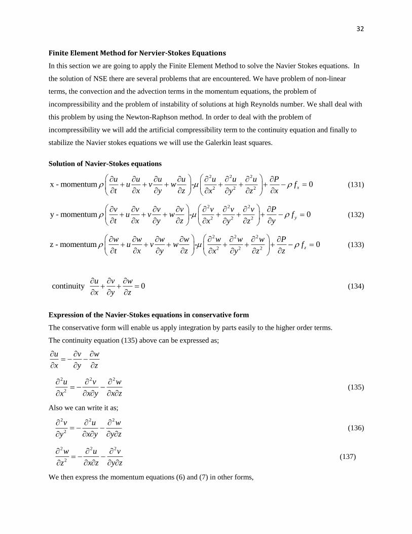
Finite Element Method for Nervier-Stokes Equations

In this section we are going to apply the Finite Element Method to solve the Navier Stokes equations. In

the solution of NSE there are several problems that are encountered. We have problem of non-linear

terms, the convection and the advection terms in the momentum equations, the problem of

incompressibility and the problem of instability of solutions at high Reynolds number. We shall deal with

this problem by using the Newton-Raphson method. In order to deal with the problem of

incompressibility we will add the artificial compressibility term to the continuity equation and finally to

stabilize the Navier stokes equations we will use the Galerkin least squares.

Solution of Navier-Stokes equations

2 2 2

2 2 2x - momentum - 0x

u u u u u u u Pu v w f

t x y z xx y z

(131)

2 2 2

2 2 2y - momentum - 0y

v v v v v v v Pu v w f

t x y z yx y z

(132)

2 2 2

2 2 2z - momentum - 0z

w w w w w w w Pu v w f

t x y z zx y z

(133)

continuity 0u v w

x y z

(134)

Expression of the Navier-Stokes equations in conservative form

The conservative form will enable us apply integration by parts easily to the higher order terms.

The continuity equation (135) above can be expressed as;

u v w

x y z

2 2 2

2

u v w

x y x zx

(135)

Also we can write it as;

2 2 2

2

v u w

x y y zy

(136)

2 2 2

2

w u v

x z y zz

(137)

We then express the momentum equations (6) and (7) in other forms,

33

Momentum equation in x – direction

The equation (132) above can be expressed as;

2 2 2 2

2 2 2 2-2 - 0x

u u u u u u u u Pu v w f

t x y z xx x y z

(138)

Replacing equation (136) into equation (139), we obtain;

2 2 2 2 2

2 2 2-2 - 0x

u u u u u v w u u Pu v w f

t x y z x y x z xx x z

(139)

We factorize the above equation to obtain;

- 2 - 0x

u u u u u v u w uu v w P f

t x y z x x y x y z x z

(140)

Momentum equation in y – direction

Similarly equation (133) can also be written in different forms. The equation above can be expressed as;

2 2 2 2

2 2 2 2-2 - 0y

v v v v v v v v Pu v w f

t x y z yy y y z

(141)

Replacing equation (137) into equation (142), we obtain;

2 2 2 2 2

2 2 2-2 - 0 y

v v v v v u w v v Pu v w f

t x y z x y y z yy x z

(142)

We factorize the above equation to obtain;

2 2 2 2

2 2- 2 - 0 y

v v v v v u w v vu v w P f

t x y z y y x y y z x z

(143)

Momentum equation in z – direction

Similarly equation (134) can also be written in different forms. The equation above can be expressed as;

2 2 2 2

2 2 2 2-2 - 0z

w w w w w w w w Pu v w f

t x y z wz x y z

(144)

Replacing equation (138) into equation (145), we obtain;

2 2 2 2 2

2 2 2-2 - 0z

w w w w w w w u v Pu v w f

t x y z x z y z wz x y

(145)

We factorize the above equation to obtain;

34

- 2 - - 0z

w w w w w w u w vu v w P f

t x y z z z x x z y y z

(146)

Therefore the new forms of the momentum equations are given by;

x - momentum

- 2 0x

u u u u v u u wu v w p f

x y z x x y x y z z x

(147)

y - momentum

- 2 0y

v v v v v u w vu v w p f

x y z y y x x y z y z

(148)

z - momentum

- 2 0z

w w w w u w w vu v w p f

x y z z z x z x y y z

(149)

continuity 0u v w

x y z

(150)

The above new form of the Stokes equations is more suitable to derive the weak form of the Stokes

equations.

Construction of approximate solution

In this section we are going to come up with the approximate solutions to the above differential equations.

the approximate solution to be chosen need to be C0 continuous, i.e. only the zero order derivative, but not

higher order, this is because higher order derivative makes the calculation complicated especially when

dealing with 2D and 3D problems. The approximate solution for the above differential equations is given

by; , , and u v w p

1 1 1

1

( , ) ( , , ) ( ), ( , ) ( , , ) ( , ) and w( , ) ( , , ) ( )

( , ) ( , , ) ( )

n n n

i i i i i i

j j j

n

i i

j

u x y x y z u t v x y x y z v x y x y x y z w t

P x y x y z p t

(151)

In this project for simplicity, we will use u, v, w and p in place of , , and u v w p respectively. Therefore

(151) becomes;

1 1 1

1

( , , ) ( ), ( , , ) ( , ) and ( , , ) ( )

( , , ) ( )

n n n

i i i i i i

j j j

n

i i

j

u x y z u t v x y z v x y w x y z w t

P x y z p t

(152)

35

Since equations in (153) are approximations, when we replace them in equations (148 – 151), the right

hand of the equations will not be equal to zero but to a residual R.

x - momentum

- 2 x

u u u u u v u u wu v w p f R

t x y z x x y x y z z x

(153)

y - momentum

- 2 y

v v v v v v u w vu v w p f R

t x y z y y x x y z y z

(154)

y - momentum

- 2 z

w w w w w u w w vu v w p f R

t x y z z z y z x y y z

(155)

continuity u y w

Rx y z

(156)

From the above equations, the residual is the difference between the exact solution and the approximate

solution. Therefore, to come up with a good approximation, we need to minimize the residual, i.e. the

smaller the residual, the more close the approximate solution to the exact solution.

To minimize the residual, there are several methods which include; the method of variation and weighted

residual. In this project, we will use the method of weighted residual. To minimize the residual, this

method uses the following weighted function;

( , ) ( , ) 0R x y w x y d

(157)

Where W(x, y) is a weight function and R(x, y) is a residual function as shown in equations (154 – 157).

As per the procedure of weighted residual approach, we will use two weight functions Q and w for

continuity and momentum equations respectively.

Replacing equations (154 – 157) in (158) we obtain;

x - momentum

2

0

v

x

u u u u u v uw u v w p

t x y z x x y x y

u wf dv

z z x

(158)

36

y - momentum

- 2

0

v

y

v v v v v v uw u v w p

t x y z y y x x y

w vf dv

z y z

(159)

z - momentum

- 2

0

v

z

w w w w w u ww u v w p

t x y z z z y z x

w vf dv

y y z

(160)

continuity 0v

u y wQ dv

x y z

(161)

For the purpose of finite element method formulation, we use Galerkin criterion, where the weight

functions are chosen to be the same as shape functions. Therefore in this case, we choose the weight

functions as; in continuity equation, we replace the weight function is replaced by, j jQ while in

momentum equation, is replaced by, i iw . Replacing the weight functions above and the

approximation functions (153) in equations (159 – 162), we obtain;

2 2 2 2 2

2 2 2

-momentum

2

+

T T T TT T T T

v v

T T T T T

v

T

xv v

x

dv u v w u dvt x y z

u u u v w dvx y z xx y z

p dv f dvx

(162)

2 2 2 2 2

2 2 2

y - momentum

2

+

T T T TT T T T

v v

T T T T T

v

T

yv

dv u v w v dvt x y z

v v v u w dvx y y zy x z

p dv fy

vdv

(163)

37

2 2 2 2 2

2 2 2

z - momentum

2

+

T T T TT T T T

v v

T T T T T

v

T

yv v

dv u v w w dvt x y z

w w w u v dvx z y zz x y

p dv f dvz

(164)

continuity

0T T T

vu v w dv

x y z

(165)

To ensure continuity of the field variable, in the next section we will choose appropriate shape functions.

We will discuss this in the next chapter.

Integration by parts in three dimension is known as Gauss divergence theorem and is given by,

v A Au dv u v n dA v udv v (166)

Applying equation (162) above, in equations (159 – 162) and re – arranging the terms, we obtain the weak

form of 3 dimension Navier-Stokes equation as;

-momentum

+ 2

+

T T T TT T T T

v v

T T T

v

T T

v

x

dv u v w u dvt x y z

udvx x y y z z

v w dv px y x z

T

xv v

dv f dvx

(167)

y-momentum

+ 2

+

T T T TT T T T

v v

T T T

v

T TT

v

dv u v w vdvt x y z

vdvx x y y z z

u w dv py x y z y

yv v

dv f dv

(168)

38

z - momentum

+ 2

+

T T T TT T T T

v v

T T T

v

T T

v

dv u v w wdvt x y z

wdvx x y y z z

u v dv pz x z y z

T

zv v

dv f dv

(169)

continuity

0T T T

vu v w dv

x y z

(170)

The above four equations are the weak form of the Navier – Stokes equations. To write the equations in

matrix form we determine some coefficient matrix formulae as follows;

1. Mass matrix

T

vM dv (171)

2. Convective matrix

, ,

T T TT T T

vC u v w u v w dv

x y z

(172)

3. Diffusive matrix

T

ijv

i j

K dvx x

(173)

4. Gradient matrix

T

iv

i

Q dvx

(174)

5. Force vector

ij iv

K f dv (175)

Substituting the above coefficient matrix formulae in the above equations, we obtain the following matrix

form of the weak statement;

39

11 22 33 13 13 1

21 11 22 33 23 2

31 32 11 22 33 3

1 2 3

M 0 0 0 ( , , ) 0 0 0

0 0 0 0 ( , , ) 0 0

0 0 0 0 0 ( , , ) 0

0 0 0 0 0 0 0 ( , , )

2K K K K K

K K 2K K K

K K K K 2K

0T T T

u C u v w u

M v C u v w v

M w C u v w w

p C u v w p

Q

Q

Q

Q Q Q

1

2

3

0

u F

v F

w F

p

(176)

From the above equation, we notice that;

1. There is a zero appearing in the diagonal of the mass matrix due to incompressibility constrain

2. The convection matrix contains non-linear terms; this can lead to unstable solution in convection

dominated flows.

In order to solve the matrix above we start by addressing the two above problems; to do this we will use

the methods of artificial compressibility and the Galerkin Stabilization method.

Artificial compressibility

The zero appearing on the diagonal is due to the incompressibility condition, u 0 .The idea behind

this technique is to convert an elliptical problem into hyperbolic by introducing an artificial term in the

continuity equation. Using this technique the alternative form of the continuity equation (1) is given by;

0 u v w

t x y z

The equation above is the artificial continuity equation,

is the artificial density and artificial compresibility such that P

. The additional term in the

equation above will not greatly affect the solutions since as calculation progresses and become

independent of time the term will disappear.

The weak form of the above equation becomes;

0v

P u v wQ dv

t x y z

(177)

We define a new matrix for this artificial equation. From the above equation the pressure matrix is

T

pv

M dv . Therefore the matrix (173) becomes

40

11 22 33 13 13 1

21 11 22 33 23 2

31 32 11 22 33 3

1 2 3

M 0 0 0 ( , , ) 0 0 0

0 0 0 0 ( , , ) 0 0

0 0 0 0 0 ( , , ) 0

0 0 0 0 0 0 ( , , )

2K K K K K

K K 2K K K

K K K K 2K

p

T T

u C u v w u

M v C u v w v

M w C u v w w

M p C u v w p

Q

Q

Q

Q Q Q

1

2

3

0 0T

u F

v F

w F

p

(178)

This matrix is now not singular.

.

0T T T

T

v

Pu v dv

t x y z

(179)

Therefore33 33K 0, K

j

ij ij j

ss d

t

, the matrix will now not be singular

Taylor Galerkin stabilization technique

Incompressible Navier – Stokes equations has non – linear unsymmetrical convective terms. As the

Reynold number increases in high velocity flows, these terms start dominating the flow field inducing

oscillations in it thus making the solutions unstable.

This method involves writing higher order time derivative of Taylor series in terms of spatial derivatives

from governing partial differential equations. Taylor Galerkin is applied only on convective term only in

Navier – Stokes – equation. The derivation of the Taylor Galerkin method for Navier- Stokes equations is

as shown in appendix A.

We will consider derivation of Taylor Galerkin technique for Navier – Stoke equation. To avoid

tediousness during derivation, we consider the vector form of the Navier – Stokes equations. Although

this method can be applied to the entire N-S-E, only convective terms are considered here as it’s the only

term which brings stability issues.

Taylor series expansion for n+1th time step is given by;

2 21

2. . .

2

n nn n u t u

u u tt t

(180)

The incompressible N-S-E which consists of only of convective terms are given by,

41

2 21

2. . .

2

n nn n u t u

u u tt t

(181)

The incompressible N-S-E consisting of only convective terms are given

u

t

u u (182)

The second derivative of u with respect to t is

2

2.

u u

t tt

u u u u u u (183)

2

2.

u

t

u u u (184)

Substituting (185) and (183) into (182), we obtain;

1

. . . .2

n nu u t

t

u u u u u (185)

Comparing (186) and (183), the stabilization term obtained by Taylor Galerkin method is a strong form of

Navier-Stokes equation. Thus we will obtain the weak form using the method of weighted residual and

applying integration by parts (Gauss theorem), therefore we obtain;

. .2 2

v v

v

tw twdv

w u v w dvx y z x y z

u u u u u u

u u u v v v (186)

Thus the expression of Taylor Galerkin stabilization is given by;

SecK , ,2

T T T TT

v

T T T T T

twu v w uu uv uw uv

x x x y x z y x

vv vw uw vw ww dvy y y z x z z y z z

(187)

Thus the stabilization matrix is written as

SecK , ,2

T T T TT

v

T T T T T

tu v w uu uv uw uv

x x x y x z y x

vv vw uw vw ww dvy y y z x z z y z z

(188)

42

Therefore the stabilization matrix become will become;

11 22 33 13 13 1

21 11 22 33 23 2

31 32 11 22 33 3

1 2 3

M 0 0 0 ( , , ) 0 0 0

0 0 0 0 ( , , ) 0 0

0 0 0 0 0 ( , , ) 0

0 0 0 0 0 0 ( , , )

2K K K K K

K K 2K K K

K K K K 2K

p

T T

u C u v w u

M v C u v w v

M w C u v w w

M p C u v w p

Q

Q

Q

Q Q Q

1

2

3

0

K , , 0 0 0

0 K , , 0 0

0 0 K , , 0

00 0 0 0

T

TG

TG

TG

u

v

w

p

u Fu v w

v Fu v w

w Fu v w

p

(189)

This is the final weak form of incompressible N-S-E which will be discretized . Now in the next section

we concentrate on finding suitable interpolation functions, and .

Choice of interpolation functions

Accuracy and the computational efficiency of solutions depend mostly on the choice of shape functions.

The choice of interpolation function for pressure is constrained by the role of pressure. The pressure here

serves only as a Lagrange multiplier that serves to enforce the incompressibility constraint on the velocity

field, therefore in order to prevent an over-constrained system of discretized equations; interpolation used

for pressure must be at least one order lower than that of velocity.

Therefore accurate solutions can only be obtained for both velocity and pressure fields by using unequal

interpolation in such a way that the shape functions associated with velocity variables are one order

higher than those associated with pressure. Both pressure and velocity need to be at least C1 continuous.

In this project, first order (linear) shape functions is selected for pressure and second order quadratic

shape function is selected for velocity variables.

43

To get the shape function, in this section we consider a tetrahedral element, however we will not derive

the shape functions, and we shall just import them. The quadratic shape function is obtained from 10

node tetrahedron as shown;

Figure 11: A ten node tetrahedron element

The quadratic coordinate Li is given as;

1 1

2 2

3 3

4 4

1 2

2 3

1 3

1 4

2 4

3 4

2 1

2 1

2 1

2 1

4

4

4

4

4

4

L l

L l

L l

L l

L L

L L

L L

L L

L L

L L

(190)

Similarly the linear shape functions is obtained from a 4 node tetra element as shown below,

Figure 12: A four node tetra element

44

1

2

3

4

L

L

L

L

(191)

The natural coordinates 1 2 3 4, L , L and L L are functions of the Cartesian coordinates and are given as

shown below;

1 1 1 1 1 2 2 2 2 2

3 3 3 3 3 4 4 4 4 4

6 , 6

6 , 6

L a b x c y d z V L a b x c y d z V

L a b x c y d z V L a b x c y d z V

(192)

The derivatives of the above functions are given by;

, where j = x, y, z and i = 1, 2, . . 46

i i

j

L b

x v

(193)

In the equations above the coefficients ai, bi, ci and did are given by;

2 2 2 2 2

1 3 3 3 1 3 3

4 4 4 4 4

2 2 2 2

1 3 3 1 3 3

4 4 4 4

1

b 1

1

1 1

1 d 1

1 1

x y z y z

a x y z y z

x y z y z

x z x y

C x z x y

x z x y

(194)

Other constants can be calculated by using cyclic permutation of subscripts 1, 2, 3, and 4 is defined

counter-clockwise.

The volume V of an element can be found by using

1 1 1

2 2 2

3 3 3

4 4 4

1

11

16

1

x y z

x y zV

x y z

x y z

(195)

Now after gathering the necessary information about the quadratic and linear shape functions we

substituted in the coefficient matrices. Before we replace the shape functions into the coefficient matrices,

we first transform them into matrices.

45

Transformation of interpolation functions

Form (191), the vector form of interpolation function can be transformed to a new matrix that consists of

the coefficient matrix [A] and the vector form of matrix {R} as expressed below;

1

2

3

4

1 2

2 3

1 3

1 4

2 4

3 4

A

1 0 0 0 1 0 1 1 0 0

0 1 0 0 1 1 0 0 1 0

0 0 1 0 0 1 1 0 0 1

0 0 0 1 0 0 0 1 1 1

0 0 0 0 4 0 0 0 0 0

0 0 0 0 0 4 0 0 0 0

0 0 0 0 0 0 4 0 0 0

0 0 0 0 0 0 0 4 0 0

0 0 0 0 0 0 0 0 4 0

0 0 0 0 0 0 0 0 0 4

L

L

L

L

L L

L L

L L

L L

L L

L L

R

(196)

Coefficient matrices construction

1. Mass matrixT

vM dv . We take the new matrix transformation into the mass matrix and

integrate this form by using the exact integral formula of

1 2 3

! ! !2

2 !

a b c

v

a b cM L L L dA A

a b c

2. The mass matrix MP

1 T

pv

M dv

From the above matrix we find that;

21 1 1 2 1 3 1 4

22 2 1 2 1 2 2 4

1 2 3 4 23 3 1 3 2 3 3 4

24 4 1 4 2 4 3 4

T

L L L L L L L L

L L L L L L L LL L L L

L L L L L L L L

L L L L L L L L

(197)

46

2

1 1 2 1 3 1 4

2

2 1 2 1 2 2 4

2

3 1 3 2 3 3 4

2

4 1 4 2 4 3 4

we will let

2 1 1 1

1 2 1 1G

1 1 2 112

1 1 1 2

v

L L L L L L L

L L L L L L L Adv

L L L L L L L

L L L L L L L

(198)

2

1 1 2 1 3 1 4

2

2 1 2 1 2 2 4

2

3 1 3 2 3 3 4

2

4 1 4 2 4 3 4

1 1Gp

v

L L L L L L L

L L L L L L LM dv

L L L L L L L

L L L L L L L

(199)

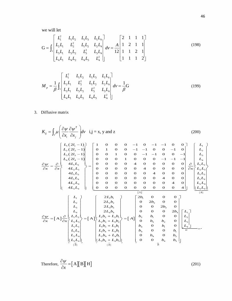
3. Diffusive matrix

i,j = x, y and zT

ijv

i j

K dvx x

(200)

1 1

2 2

3 3

4 4

1 2

2 3

1 3

1 4

2 4

3 4

2 1 1 0 0 0 1 0 1 1 0 0

2 1 0 1 0 0 1 1 0 0 1 0

2 1 0 0 1 0 0 1 1 0 0 1

2 1 0 0 0 1 0 0 0 1 1 1

4 0 0 0 0 4 0 0 0 0 0

4 0 0 0 0 0 4 0 0 0 0

4 0 0 0 0 0 0 4 0 0 0

4 0 0 0 0 0 0 0 4 0 0

4 0 0 0 0 0 0 0

4

L l

L l

L l

L l

L L

L Lx x

L L

L L

L L

L L

1

2

3

4

1 2

2 3

1 3

1 4

2 4

3 4

A

1

2

3

4

1 2

2 3

1 3

1 4

2 4

3 4

0 4 0

0 0 0 0 0 0 0 0 0 4

A

R

L

L

L

L

L L

L Lx

L L

L L

L L

L L

L

L

L

L

L L

L Lx x

L L

L L

L L

L L

1 1 1

2 2 2

3 3 3

4 4 4

1 2 2 1 2 1

2 3 3 2 3 2

1 3 3 1 4 1

1 4 4 1 4 1

2 4 4 1 4 2

3 4 4 3

2 2 0 0 0

2 0 2 0 0

2 0 0 2 0

2 0 0 0 2

0 0A

0 0

0 0

0 0

0 0

0 0

R R

L b b

L b b

L b b

L b b

L b L b b bA

L b L b b b

L b L b b b

L b L b b b

L b L b b b

L b L b b

1

2

3

4

4 3

H

B

L

L

L

L

b

Therefore, A B Hx

(201)

47

Similarly,

A C H , A D Hy x

(202)

Therefore equation (201) can be written as

T T T

11 = A B A B H H AT

v AK dv d

x x

(203)

From equation (199) equation (204) can be written as

T T

11 A B G A BK (204)

Similarly

T T T T T T

22 33 12

T T T T T T

32 23 13

T T T T

21 31

A C G C A A D G D A A B G C A

A D G C A A C G D A A B G D A

A C G A B A D G A B

K K K

K K K

K K

(205)

4. The stabilized mass matrix

SecK , ,2

T T T T

v

T T T T T

tu v w uu uv uw uv

x x x y x z y x

vv vw uw vw ww dvy y y z x z z y z z

(206)

T T T T T T

T T T T T T

T T T T

( , ) A B G A B A B G C A A B G D A 2

+ A C G A B A C G C A A C G D A

A D G A B A D G C A A D G

se

tK u v uu uv uw

uv vv vw

wu vw ww

T TD A

(207)

5. Stiffness gradient matrix, T

iv

i

Q dvx

48

1

2

3

A B H H A B G

A C H H A C G

A D H H A D G

TT

v V

TT

v V

TT

v V

Q dv dvx

Q dv dvy

Q dv dvz

(208)

Mass convective matrix

, ,T T T

T T T

vC u v w u v w dv

x y z

(209)

The convective matrices are given by;

T T

T T

T T

A A A B R R H

A A A C R R H

A A A D R R H

TT

xv V

TT

yv V

TT

zv V

C u u dv v dvx

C v v dv v dvy

C w w dv w dvz

(210)

Or

T T

T

2 2A A A B F A A A C F

540 540

2A A A D F

540

x y

z

A AC u C v

AC w

(211)

Now this is the final general form of the finite element matrix formula.

Equation (190) still contains non-linear terms. To line arise the non-linear terms we use the Newton

Raphson method on the non-linear term only,

11 22 33 12 13 1 1

21 11 22 33 23 2 2

31 32 11 22 33 3 3

1 2 3

C+2K K K K K

K C+K 2K K K

K K C+K K 2K

0 0

se

se

se

T T T

K Q u F

K Q v F

K Q w F

Q Q Q p

(212)

49

Or

( ) UK u F (213)

We now transform the equation above into Newton – Raphson form as,

( ) ( ) U- 0R u K u F (214)

Newton-Raphson method is based on truncated Taylor series expansion of R(U) about the known solution

Un

20 ( ) 0R

R U U UU

(215)

Where, 1n nU U U . Omitting the terms of order higher, we obtain,

1 1( )n n n n n nRR U U U J U U U

U

(216)

Where J is the Jacobean

By solving equation (217), we get

1 1n n n nU U J U R U (217)

Applying equation (214) to (216), we obtain,

11 12 21 22

13 23 31 32 33

1 1 2 3 11 22 33 12 13 1 1

2 1 2 3 11 22 33 21 23

2

+2

2

s S S S

S S S S S

R C u u C v u C w u K K K u K v K w Q p F

tK uu u K uv u K vu u K vv u

K uw u K vw u K wu u K wv u K ww u

R C u v C v v C w v K K K v K u K

11 12 21 22

13 23 31 32 33

11 12

1 2

3 1 2 3 11 22 33 31 32 1 3

+2

2

+2

s S S S

S S S S S

s S S

w Q p F

tK uu v K uv v K vu v K vv v

K uw v K vw v K wu v K wv v K ww v

R C u w C v w C w w K K K w K u K v Q p F

tK uu w K uv w K

21 22

13 23 31 32 33

S

S S S S S

vu w K vv w

K uw w K vw w K wu w K wv w K ww w

(218)

The Jacobian in (218) is given by;

50

RJ

U

(219)

Now to evaluate the above matrix, we substitute (220) into it. We get the derivative of the stiffness matrix

in the Newton-Raphson form to be,

1 1 1 1

2 2 2 2

3 3 3 3

4 4 4 4

R R R R

u v w p

R R R R

u v w pRJ

R R R RU

u v w p

R R R R

u v w p

(220)

11 12 21 22

13 23 31 32 33

11 12 21

1

1 2 3 11 22 33

2

1 2 3 11 22 33

2

+2

2

+2

s S S S

S S S S S

s S S S

RC u C v C w K K K

u

tK uu K uv K vu K vv

K uw K vw K wu K wv K ww

RC u C v C w K K K

v

tK uu K uv K vu K

22

13 23 31 32 33

11 12 21 22

13 23 31 32 33

3

1 2 3 11 22 33

2

+2

S S S S S

s S S S

S S S S S

vv

K uw K vw K wu K wv K ww

RC u C v C w K K K

w

tK uu K uv K vu K vv

K uw K vw K wu K wv K ww

(221)

Similarly we derive,

3 3 3 31 4 2 4 1 2 1 2, , , , , , , , , , , R R R RR R R R R R R R

v v v u u u w w w p p p

We now substitute (220) into (218) to get;

51

1 1 1 1

2 2 2 2

1

3 3 3 3

4 4 4 4

n n n

R R R R

u v w p

R R R R

u v w pR U U U

R R R R

u v w p

R R R R

u v w p

(222)

Thus (214) can be replaced by;

1 1 1 1

1 112 2 2 2

1 12

1 133 3 3 3

1 14

4 4 4 4

where,

n n

n n

n n

n n

R R R R

u v w p

Ru uR R R R

Ru v w p v v

RR R R R w w

u v w p Rp p

R R R R

u v w p

1

1

1

1

n n

n n

n n

n n

u u

v v

w w

p p

(223)

We substitute (225) into (190) to obtain

1 1 1 1

112 2 2 2

12

133 3 3 3

14

4 4 4 4

M 0 0 0

0 0 0

0 0 0

0 0 0

n

n

n

np

R R R R

u v w p

Ru uR R R R

M Rv u v w p v

M RR R R Rw w

M u v w p Rp p

R R R R

u v w p

(224)

Or M K U U U R (225)

To derive the solution of the time approximation method using implicit method, we start by time

derivative term in the above equation

1n nU U U

t t

U (226)

52

Substituting (228) into (227) we obtain,

1 1 1 1n n n n nM U t R U K U U M U

(227)

Once we have obtained the final form of the solution of Navier-Stokes equation, we now apply it to flows

through pipe.

Finite element solutions and programming

Now after obtaining the final form of Navier – Stokes equations, we use a matlab program to

solve the equation. The Matlab program is given in appendix A. to test the Matlab program, we

first apply it to lid driven cavity problem.

Figure 13: Lid driven cavity problem

53

4. Results and Conclusion After applying the computer program developed to lid-driven the following results were obtained.

Figure 14: Solutions to lid driven cavity problem

Figure 15: Solutions to lid driven cavity problem

54

Since these results are true according to those published, hence the matlab program developed is correct.

After applying the Matlab program in appendix A to the above problem, the following results were

obtained.

When the graph above is rotated laterally, we obtain

From the two figures above it can be seen that uniform inlet flow develops into a parabolic profile as it

moves along the length.

55

5. Bibliography

Calves, V. (2010). Cardiovascular system. Paris.

Campbell, N. A. (1996). Biology, human physiology. University of California: Benjamin publishing

company.

Chatzizis, Y. (2008). Prediction of the localisation of high-risk cocronaary atherosclerotic plaques on the

basis of low endothelial shear stress. Harvard Medical School.

Cheng, C. (2006). Atherosclerotic lesion size and vulnerability are determined by patterns of fluid shear

stress. University medical center Rotterdam, Netherland.

Gohil, T. (2002). SIMULATION OF OSCILLATORY FLOW IN AN AORTIC BIFURCATION USING FVM AND

FEM. International Journal for Numerical Methods in Fluids , India.

Gunzburger, M. D. (2013). Finite Element Methods. Paris.

J.Segerlind, L. (1976). Applied Finite Element Analysis. New York: John Wiley and Sons.

Jiajan, W. (2010). Solution of to incompressible Navier-Stokes equations by using finite element method.

University of texas.

Kazakidi, A. (2008). Computational Studies of Blood. University of London.

Kumar, D. D. (2008). Fluid mechanics and fluid Power engineering. India: S.K. Karataria and sons.

Nicolass, F. (2005). Numerial Analysis of carotid artery.

Organisation, W. H. (2011). Cardiovascular diseases.

Quarterson, A. (2002). Mathematical modelling and Numerical simulation of cardiovascular system.

switzerland.

Ritzen, R. (. (2012). Modeling of blood flow in coronary arteries with junctions. Netherlands.

Ritzen, R. (2012). Mathematical modeling of blood flow through a deformable thin-walled vessel.

Netherland.

Ruengsakulrach, P. Wall shear stress and Atherosclerosis. Thailand.

Wake, A. K. (2005). Modeling of fluid mechanics in individual human carotid arteries. Georgia.

WHO. (2002). World health report.

Xiu-YIng, K. (2008). Blood flow at arterial bifurcation. Beijing.

56

6. Table of figures

Figure 1: Circulatory system (Gohil, 2002) ................................................................................................. 1

Figure 2: Atherosclerosis plaque................................................................................................................... 2

Figure 3: wall shear stress and velocity distribution ..................................................................................... 3

Figure 4: Shape of an artery .......................................................................................................................... 8

Figure 5: Velocity distribution in a straight pipe ......................................................................................... 23

Figure 6: Stress distribution in a straight pipe ............................................................................................ 23

Figure 7: Velocity distribution at bifurcation point .................................................................................... 24

Figure 8: Velocity distribution at branch point ........................................................................................... 24

Figure 9: Stress distribution at branch point .............................................................................................. 25

Figure 10: A linear polynomial element ...................................................................................................... 26

Figure 11: A ten node tetrahedron element ................................................................................................. 43

Figure 12: A four node tetra element .......................................................................................................... 43

Figure 13: Lid driven cavity problem........................................................................................................... 52

Figure 14: Solutions to lid driven cavity problem ...................................................................................... 53

Figure 15: Solutions to lid driven cavity problem ....................................................................................... 53

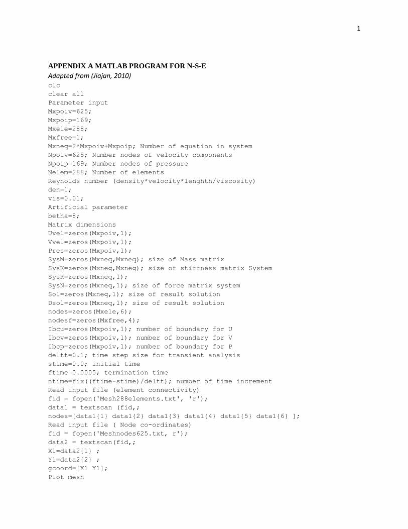
1

APPENDIX A MATLAB PROGRAM FOR N-S-E

Adapted from (Jiajan, 2010) clc

clear all

Parameter input

Mxpoiv=625;

Mxpoip=169;

Mxele=288;

Mxfree=1;

Mxneq=2*Mxpoiv+Mxpoip; Number of equation in system

Npoiv=625; Number nodes of velocity components

Npoip=169; Number nodes of pressure

Nelem=288; Number of elements

Reynolds number (density*velocity*lenghth/viscosity)

den=1;

vis=0.01;

Artificial parameter

betha=8;

Matrix dimensions

Uvel=zeros(Mxpoiv,1);

Vvel=zeros(Mxpoiv,1);

Pres=zeros(Mxpoiv,1);

SysM=zeros(Mxneq,Mxneq); size of Mass matrix

SysK=zeros(Mxneq,Mxneq); size of stiffness matrix System

SysR=zeros(Mxneq,1);

SysN=zeros(Mxneq,1); size of force matrix system

Sol=zeros(Mxneq,1); size of result solution

Dsol=zeros(Mxneq,1); size of result solution

nodes=zeros(Mxele,6);

nodesf=zeros(Mxfree,4);

Ibcu=zeros(Mxpoiv,1); number of boundary for U

Ibcv=zeros(Mxpoiv,1); number of boundary for V

Ibcp=zeros(Mxpoiv,1); number of boundary for P

deltt=0.1; time step size for transient analysis

stime=0.0; initial time

ftime=0.0005; termination time

ntime=fix((ftime-stime)/deltt); number of time increment

Read input file (element connectivity)

fid = fopen('Mesh288elements.txt', 'r');

data1 = textscan (fid,;

nodes=[data1{1} data1{2} data1{3} data1{4} data1{5} data1{6} ];

Read input file ( Node co-ordinates)

fid = fopen('Meshnodes625.txt, r');

data2 = textscan(fid,;

X1=data2{1} ;

Y1=data2{2} ;

gcoord=[X1 Y1];

Plot mesh

2

figure(1)

clf

plot(X1,Y1,’.r’,’MarkerSize’,10)

hold on

tri=nodes;

triplot(tri,X1,Y1);

Boundary condition

fid = fopen(’625BC.txt’, ’r’);

data1 = textscan(fid, ’

Ibcu=data1{1} ;

Ibcv=data1{2} ;

Ibcp=data1{3} ;

Uvel=data1{4} ;

Vvel=data1{5} ;

Pres=data1{6} ;

B.1.2 Loop for number of equations

Neq=2*Npoiv+Npoip;

Loop for initilize force vector

for i=1:Neq

SysR(i)=0;

end

Loop for initilize stiffness matrix

for i=1:Neq

for j=1:Neq

SysK(i,j)=0;

end

end

Loop for initilize mass matrix

for i=1:Neq

for j=1:Neq

SysM(i,j)=0;

end

end

B.1.3 Mass matrix construction

[SysM]=TRInew1(Npoiv,Nelem,den,vis,gcoord,nodes,SysM);

B.1.4 Initial guess value input

for i=1:Npoiv loop for velocity components

Sol(i)=0.0356;

Sol(i+Npoiv)=0.00032272;

end

for i=1:Npoip loop for pressure

Sol(i+Npoiv+Npoiv)=0.998;

end

B.1.5 Numerical programming codes ”AC Backward Newton-Raphson Method”

SysK=SysM+deltt*SysK;

sum=zeros(ntime,1);

check=zeros(ntime,1);

for it=1:ntime iteration in each time plane

for iter=1:100 number of iterations

3

Newton-Raphson Non-linear matrix construction

[SysK,SysR]=TRI(Npoiv,Npoip,Nelem,Nfree,Neq,den,vis,

gcoord,nodes,SysK,SysR,Sol);

Backward different scheme

SysN=deltt*SysR+SysM*Sol;

apply boundary condition call ”ApplyBC55”

[SysK, SysN]=ApplyBC55(Npoiv,Npoip,Neq,Ibcu,Ibcv,Ibcp,

SysK,SysN,Uvel,Vvel,Pres);

Solve equations

Sol=inv(SysK)*SysN

iteration checking

for i=1:Npoip

Psol(i,it)=Sol(2*Npoiv+i);

Psol(i,it+1)=Sol(2*Npoiv+i);

end

Iteration=iter

end

Ntime=it

end

Convergence Checking

for it=1:ntime

for i=1:Npoip

sum(it)=sum(it)+(Psol(i,it+1)-Psol(i,it))/deltt;

check(it)=abs(1/betha*sum(it));

end

Check(it,1)=check(it);

if(abs(check(it))¡1e-6)

fprintf(’Pressure converged in iterations’);

break;

end

Ntime=it;

end

B.1.6 Output

plot the history of convergence

figure(2)

time=0:deltt:Ntime*deltt;

semilogy(time,(Check(:,1)),’-’);

xlabel(’Time’)

ylabel(’Pressure convergence’)

title(’Convergence history’)

Print output

for i=1:Npoiv

Uvelocity(i)=Sol(i);

Vvelocity(i)=Sol(Npoiv+i);

end

for i=1:Npoip

Pressure(i)=Sol(i+2*Npoiv);

end

Velocity=[Uvelocity’ Vvelocity’]

4

Pressure=Pressure’

plot velocity vector

x=X1;

y=Y1;

scale=2;

u=Uvelocity’;

v=Vvelocity’;

figure(3)

quiver ( x, y, u, v, scale, ’b’ );

axis equal

hold on

k = convhull ( x, y );

plot ( x(k), y(k), ’r’ );

hold on

xmin = min ( x );

xmax = max ( x );

ymin = min ( y );

ymax = max ( y );

delta = 0.05 * max ( xmax - xmin, ymax - ymin );

plot ( [ xmin - delta,xmax + delta,xmax + delta,xmin - delta, xmin - delta ],

[ ymin - delta, ymin - delta,ymax + delta,ymax + delta,ymin - delta ],

’w’ );

hold off

B.2 Sub programming ”Functions”

B.2.1 Mass matrix Coefficient Function ”TRInew1”

function [SysM]=TRInew1(Npoiv,Nelem,den,vis,gcoord,nodes,SysM)

A=zeros(6,6);B=zeros(6,3);C=zeros(6,3);G=zeros(3,3);

M11=zeros(6,6);M22=zeros(6,6);M33=zeros(3,3);Mele=zeros(15,15);

Rele=zeros(15,1);

Set up matrix [A]

for i=1:6

for j=1:6

A(i,j)=0;

end

end

A(1,1)=1;A(2,2)=1;A(3,3)=1;A(4,4)=4;A(5,5)=4;

A(6,6)=4;A(1,5)=-1;A(1,6)=-1;A(2,4)=-1;A(2,6)=-1;

A(3,4)=-1;A(3,5)=-1;

betha=8;

Anew=vis/den; kinematic viscosity

for iel=1:Nelem loop for the total number of elements

II=nodes(iel,1);

JJ=nodes(iel,2);

KK=nodes(iel,3);

LL=nodes(iel,4);

MM=nodes(iel,5);

84

NN=nodes(iel,6);

x1=gcoord(II,1); y1=gcoord(II,2);

5

x2=gcoord(JJ,1); y2=gcoord(JJ,2);

x3=gcoord(KK,1); y3=gcoord(KK,2);

Area=0.5*((x2*y3)+(x1*y2)+(x3*y1)-(x2*y1)-(x1*y3)-(x3*y2));

Area2=2*Area;

b1=(y2-y3)/Area2;

b2=(y3-y1)/Area2;

b3=(y1-y2)/Area2;

c1=(x3-x2)/Area2;

c2=(x1-x3)/Area2;

c3=(x2-x1)/Area2;

Compute matrix [B] [C] and [G]

for i=1:6

for j=1:3

B(i,j)=0;

C(i,j)=0;

end end

B(1,1)=2*b1;B(5,1)=b3;B(6,1)=b2;B(2,2)=2*b2;

B(4,2)=b3; B(6,2)=b1; B(3,3)=2*b3; B(4,3)=b2; B(5,3)=b1;

C(1,1)=2*c1; C(2,2)=2*c2; C(3,3)=2*c3; C(5,1)=c3;

C(5,3)=c1; C(6,1)=c2; C(6,2)=c1; C(4,2)=c3; C(4,3)=c2;

Fac=Area/12;

Fac2=2*Fac;

G(1,1)=Fac2; G(2,2)=Fac2; G(3,3)=Fac2; G(1,2)=Fac; G(1,3)=Fac;

G(2,1)=Fac; G(2,3)=Fac; G(3,1)=Fac; G(3,2)=Fac;

Set up mass matrix

D(1,1)=12; D(2,2)=12; D(3,3)=12; D(4,4)=2; D(5,5)=2; D(6,6)=2;

D(1,2)=2; D(1,3)=2; D(1,4)=1; D(1,5)=3; D(1,6)=3; D(2,3)=2; D(2,4)=3;

D(2,5)=1; D(2,6)=3; D(3,4)=3; D(3,5)=3; D(3,6)=1; D(4,5)=1;

D(4,6)=1; D(5,6)=1;

for i=1:6

for j=1:6

D(j,i)=D(i,j);

end

end

M11=2*Area/360*den*A*D*A’;

M22=2*Area/360*den*A*D*A’;

M33=G/betha;

Then the matrix (15x15) on LHS is

for i=1:15

for j=1:15

Mele(i,j)=0;

end

end

Final local mass matrix

for i=1:6

for j=1:6

Mele(i,j)=M11(i,j);

Mele(i+6,j+6)=M22(i,j);

end

6

end

for i=1:3

for j=1:3

Mele(i+12,j+12)=M33(i,j);

end

end

Assembly Global mass matrix

[SysM]=ASSEMBLEnew1(iel,nodes,Mele,SysM,Npoiv);

end

B.2.2 Assembly to Global mass matrix function ”ASSEMBLEnew1”

function [SysM]=ASSEMBLEnew1(iel,nodes,Mele,SysM,Npoiv)

Contribution of coeficients assocoated with u,v velocities

for i=1:6

for j=1:6

II=nodes(iel,i);

JJ=nodes(iel,j);

k=i+6;

l=j+6;

KK=Npoiv+II;

LL=Npoiv+JJ;

SysM(II,JJ)=SysM(II,JJ)+Mele(i,j);

SysM(II,LL)=SysM(II,LL)+Mele(i,l);

SysM(KK,JJ)=SysM(KK,JJ)+Mele(k,j);

SysM(KK,LL)=SysM(KK,LL)+Mele(k,l);

end

end

Contribution of coeficients assocoated with P pressure

for i=1:3

for j=1:3

II=nodes(iel,i);

JJ=nodes(iel,j);

k=i+12;

l=j+12;

KK=2*Npoiv+II;

LL=2*Npoiv+JJ;

SysM(II,LL)=SysM(II,LL)+Mele(i,l);

SysM(KK,LL)=SysM(KK,LL)+Mele(k,l);

end

end

B.2.3 Local stiffness coefficient matrix function ”TRI”

function [SysK,SysR]=TRI(Npoiv,Npoip,Nelem,Neq,den,vis,

gcoord,SysK,SysR,Sol);

A=zeros(6,6);B=zeros(6,3);C=zeros(6,3);G=zeros(3,3);F=zeros(6,6,3);

Uele=zeros(6,1);Vele=zeros(6,1);Pele=zeros(3,1);

Sxx=zeros(6,6);Sxy=zeros(6,6);Syx=zeros(6,6);Syy=zeros(6,6);

Qx=zeros(3,6);Qy=zeros(3,6);Qxt=zeros(6,3);Qyt=zeros(6,3);

ABGXUG=zeros(6,6);AGBXUG=zeros(6,6);AGBYVG=zeros(6,6);

ABGYVG=zeros(6,6);ABGXVG=zeros(6,6);ABGYUG=zeros(6,6);

Gxx=zeros(6,6);Gyy=zeros(6,6);Alx=zeros(6,6);Aly=zeros(6,6);

7

Akele=zeros(15,15);Rele=zeros(15,1);FX=zeros(6,1);FY=zeros(6,1);

FI=zeros(3,1);

Set up matrix [A]

for i=1:6

for j=1:6

A(i,j)=0;

end

end

A(1,1)=1; A(2,2)=1; A(3,3)=1; A(4,4)=4; A(5,5)=4;

A(6,6)=4; A(1,5)=-1; A(1,6)=-1; A(2,4)=-1; A(2,6)=-1;

A(3,4)=-1; A(3,5)=-1;

Anew=vis/den;

for iel=1:Nelem loop for the total number of elements

II=nodes(iel,1);

JJ=nodes(iel,2);

KK=nodes(iel,3);

LL=nodes(iel,4);

MM=nodes(iel,5);

NN=nodes(iel,6);

x1=gcoord(II,1); y1=gcoord(II,2);

x2=gcoord(JJ,1); y2=gcoord(JJ,2);

x3=gcoord(KK,1); y3=gcoord(KK,2);

Area=0.5*((x2*y3)+(x1*y2)+(x3*y1)-(x2*y1)-(x1*y3)-(x3*y2));

Area2=2*Area;

b1=(y2-y3)/Area2;

b2=(y3-y1)/Area2;

b3=(y1-y2)/Area2;

c1=(x3-x2)/Area2;

c2=(x1-x3)/Area2;

c3=(x2-x1)/Area2;

Compute matrix [B] [C] and [G]

for i=1:6

for j=1:3

B(i,j)=0;

C(i,j)=0;

end

end

B(1,1)=2*b1; B(5,1)=b3; B(6,1)=b2; B(2,2)=2*b2;

B(4,2)=b3; B(6,2)=b1; B(3,3)=2*b3; B(4,3)=b2;

B(5,3)=b1; C(1,1)=2*c1; C(2,2)=2*c2; C(3,3)=2*c3;

C(5,1)=c3; C(5,3)=c1; C(6,1)=c2; C(6,2)=c1;

C(4,2)=c3; C(4,3)=c2;

Set up [G] matrix

Fac=Area/12;

Fac2=2*Fac;

G(1,1)=Fac2; G(2,2)=Fac2; G(3,3)=Fac2; G(1,2)=Fac; G(1,3)=Fac;

G(2,1)=Fac; G(2,3)=Fac; G(3,1)=Fac; G(3,2)=Fac;

Set up matrix [F]

Factor=2*Area/5040;

8

F4=Factor*4;

F6=Factor*6; F12=Factor*12; F24=Factor*24; F120=Factor*120;

F(1,1,1)=F120; F(1,2,1)=F12; F(1,3,1)=F12; F(1,4,1)=F6;

F(1,5,1)=F24; F(1,6,1)=F24; F(2,2,1)=F24; F(2,3,1)=F4;

F(2,4,1)=F6; F(2,5,1)=F4; F(2,6,1)=F12; F(3,3,1)=F24;

F(3,4,1)=F6; F(3,5,1)=F12; F(3,6,1)=F4; F(4,4,1)=F4;

F(4,5,1)=F4; F(4,6,1)=F4; F(5,5,1)=F12; F(5,6,1)=F6; F(6,6,1)=F12;

for i=1:6

for j=1:6

F(j,i,1)=F(i,j,1);

end

end

F(1,1,2)=F24; F(1,2,2)=F12; F(1,3,2)=F4; F(1,4,2)=F4;

F(1,5,2)=F6; F(1,6,2)=F12; F(2,2,2)=F120; F(2,3,2)=F12;

F(2,4,2)=F24; F(2,5,2)=F6; F(2,6,2)=F24; F(3,3,2)=F24;

F(3,4,2)=F12; F(3,5,2)=F6; F(3,6,2)=F4; F(4,4,2)=F12;

F(4,5,2)=F4; F(4,6,2)=F6; F(5,5,2)=F4; F(5,6,2)=F4; F(6,6,2)=F12;

for i=1:6

for j=1:6

F(j,i,2)=F(i,j,2);

end

end

F(1,1,3)=F24; F(1,2,3)=F4; F(1,3,3)=F12; F(1,4,3)=F4;

F(1,5,3)=F12; F(1,6,3)=F6; F(2,2,3)=F24; F(2,3,3)=F12;

F(2,4,3)=F12; F(2,5,3)=F4; F(2,6,3)=F6; F(3,3,3)=F120;

F(3,4,3)=F24; F(3,5,3)=F24; F(3,6,3)=F6; F(4,4,3)=F12;

F(4,5,3)=F6; F(4,6,3)=F4; F(5,5,3)=F12; F(5,6,3)=F4; F(6,6,3)=F4;

for i=1:6

for j=1:6

F(j,i,3)=F(i,j,3);

end

end

Extract element nodal u v and p

Uele(1)=Sol(II);

Uele(2)=Sol(JJ);

Uele(3)=Sol(KK);

Uele(4)=Sol(LL);

Uele(5)=Sol(MM);

Uele(6)=Sol(NN);

Vele(1)=Sol(II+Npoiv);

Vele(2)=Sol(JJ+Npoiv);

Vele(3)=Sol(KK+Npoiv);

Vele(4)=Sol(LL+Npoiv);

Vele(5)=Sol(MM+Npoiv);

Vele(6)=Sol(NN+Npoiv);

Pele(1)=Sol(II+Npoiv+Npoiv);

Pele(2)=Sol(JJ+Npoiv+Npoiv);

Pele(3)=Sol(KK+Npoiv+Npoiv);

Compute [sxx] [sxy] [syx] [syy] matrices

9

for IA=1:6

for IB=1:6

K11=0;

K22=0;

K12=0;

K21=0;

for i=1:6

for j=1:3

for k=1:3

for l=1:6

K11=K11+A(IA,i)*B(i,j)*A(IB,l)*B(l,k)*G(j,k);

K22=K22+A(IA,i)*C(i,j)*A(IB,l)*C(l,k)*G(j,k);

K12=K12+A(IA,i)*C(i,j)*A(IB,l)*B(l,k)*G(j,k);

K21=K21+A(IA,i)*B(i,j)*A(IB,l)*C(l,k)*G(j,k);

end

end

end

end

Sxx(IA,IB)=2*Anew*K11+Anew*K22;

Sxy(IA,IB)=Anew*K12;

Syx(IA,IB)=Anew*K21;

Syy(IA,IB)=Anew*K11+2*Anew*K22;

end

end

Compute stabilize term matrices

for IA=1:6

for IB=1:6

Ks11uu=0;

Ks112uu=0;

Ks22vv=0;

Ks222vv=0;

Ks222vu=0;

Ks222uv=0;

Ks12uv=0;

Ks12uu=0;

Ks12vu=0;

Ks12vv=0;

Ks21vu=0;

Ks21uv=0;

Ks21uu=0;

Ks21vv=0;

for i=1:6

for j=1:3

for k=1:3

for l=1:6

Ks11uu=Ks11uu+A(IA,i)*B(i,j)*A(IB,l)*B(l,k)*G(j,k)*Uele(l)*Uele(i);

Ks112uu=Ks112uu+A(IA,i)*B(l,k)*A(IB,l)*B(i,j)*G(j,k)*2*Uele(l)*Uele(i);

Ks22vv=Ks22vv+A(IA,i)*C(i,j)*A(IB,l)*C(l,k)*G(j,k)*Vele(l)*Vele(i);

Ks222vv=Ks222vv+A(IA,i)*C(l,k)*A(IB,l)*C(i,j)*G(j,k)*2*Vele(l)*Vele(i);

10

Ks12uv=Ks12uv+A(IA,i)*C(i,j)*A(IB,l)*B(l,k)*G(j,k)*Uele(l)*Vele(i);

Ks12vu=Ks12vu+A(IA,i)*C(l,k)*A(IB,l)*B(i,j)*G(j,k)*Vele(l)*Uele(i);

Ks21vu=Ks21vu+A(IA,i)*B(i,j)*A(IB,l)*C(l,k)*G(j,k)*Vele(l)*Uele(i);

Ks222vu=Ks222vu+A(IA,i)*C(i,j)*A(IB,l)*C(l,k)*G(j,k)*2*Vele(l)*Uele(i);

Ks222uv=Ks222uv+A(IA,i)*C(i,j)*A(IB,l)*C(l,k)*G(j,k)*2*Uele(l)*Vele(i);

Ks12uu=Ks12uu+A(IA,i)*C(i,j)*A(IB,l)*B(l,k)*G(j,k)*Uele(l)*Uele(i);

Ks12vv=Ks12vv+A(IA,i)*C(i,j)*A(IB,l)*B(l,k)*G(j,k)*Vele(l)*Vele(i);

Ks21uv=Ks21uv+A(IA,i)*B(i,j)*A(IB,l)*C(l,k)*G(j,k)*Uele(l)*Vele(i);

Ks21uu=Ks21uu+A(IA,i)*B(i,j)*A(IB,l)*C(l,k)*G(j,k)*Uele(l)*Uele(i);

Ks21vv=Ks21vv+A(IA,i)*B(i,j)*A(IB,l)*C(l,k)*G(j,k)*Uele(l)*Uele(i);

end

end

end

end

KS11uu(IA,IB)=Ks11uu;

KS112uu(IA,IB)=Ks112uu;

KS22vv(IA,IB)=Ks22vv;

KS222vv(IA,IB)=Ks222vv;

KS222vu(IA,IB)=Ks222vu;

KS222uv(IA,IB)=Ks222uv;

KS12uv(IA,IB)=Ks12uv;

KS12uu(IA,IB)=Ks12uu;

KS12vu(IA,IB)=Ks12vu;

KS12vv(IA,IB)=Ks12vv;

KS21vu(IA,IB)=Ks21vu;

KS21uv(IA,IB)=Ks21uv;

KS21uu(IA,IB)=Ks21uu;

KS21vv(IA,IB)=Ks21vv;

end

end

for i=1:6

for j=1:6

Kse1(i,j)=deltt/2*(KS11uu(i,j)+KS112uu(i,j)+KS22vv(i,j)+

KS12uv(i,j)+KS12vu(i,j) +KS21vu(i,j)+KS21vu(i,j));

Kse2(i,j)=deltt/2*(KS11uu(i,j)+KS22vv(i,j)+

KS12uv(i,j)+KS12uv(i,j)+KS21vu(i,j)+KS21uv(i,j)+KS222vv(i,j));

Kse3(i,j)=deltt/2*(KS12uu(i,j)+KS21uu(i,j)+KS222vu(i,j));

Kse4(i,j)=deltt/2*(KS12vv(i,j)+KS21vv(i,j)+KS222uv(i,j));

end

end

Compute [Q1] and [Q2]

for IA=1:3

for IB=1:6

Cx=0;

Cy=0;

for i=1:6

for j=1:3

Cx=Cx+A(IB,i)*B(i,j)*G(j,IA);

Cy=Cy+A(IB,i)*C(i,j)*G(j,IA);

11

end

end

Qx(IA,IB)=Cx/den;

Qy(IA,IB)=Cy/den;

end end

Then the corresponding two matrices on the upper right

for IA=1:3

for IB=1:6

Qxt(IB,IA)= -Qx(IA,IB);

Qyt(IB,IA)= -Qy(IA,IB);

end

end

Compute all matrices associated with the inertia term

for IA=1:6

for IB=1:6

Cabgxug=0;

Cagbxug=0;

Cagbyvg=0;

Cabgyvg=0;

Cabgxvg=0;

Cabgyug=0;

for i=1:6

for j=1:6

for k=1:6

for l=1:6

for m=1:3

Cabgxug=Cabgxug+A(IA,i)*A(IB,j)*A(k,l)*B(l,m)*F(i,j,m)*Uele(k);

Cagbxug=Cagbxug+A(IA,i)*A(k,j)*A(IB,l)*B(l,m)*F(i,j,m)*Uele(k);

Cagbyvg=Cagbyvg+A(IA,i)*A(k,j)*A(IB,l)*C(l,m)*F(i,j,m)*Vele(k);

Cabgyvg=Cabgyvg+A(IA,i)*A(IB,j)*A(k,l)*C(l,m)*F(i,j,m)*Vele(k);

Cabgxvg=Cabgxvg+A(IA,i)*A(IB,j)*A(k,l)*B(l,m)*F(i,j,m)*Vele(k);

Cabgyug=Cabgyug+A(IA,i)*A(IB,j)*A(k,l)*C(l,m)*F(i,j,m)*Uele(k);

end

end

end

end

end

ABGXUG(IA,IB)=Cabgxug;

AGBXUG(IA,IB)=Cagbxug;

AGBYVG(IA,IB)=Cagbyvg;

ABGYVG(IA,IB)=Cabgyvg;

ABGXVG(IA,IB)=Cabgxvg;

ABGYUG(IA,IB)=Cabgyug;

end

end

Take in system equation

for i=1:6

for j=1:6

Gxx(i,j)=ABGXUG(i,j)+AGBXUG(i,j)+AGBYVG(i,j)+Sxx(i,j)+Kse1(i,j);

12

Gyy(i,j)=ABGYVG(i,j)+AGBYVG(i,j)+AGBXUG(i,j)+Syy(i,j)+Kse2(i,j);

Alx(i,j)=ABGXVG(i,j)+Sxy(i,j)+Kse3(i,j);

Aly(i,j)=ABGYUG(i,j)+Syx(i,j)+Kse4(i,j);

end

end

Then the matrix (15x15) on LHS is

for i=1:15

for j=1:15

Akele(i,j)=0;

end

end

for i=1:6

for j=1:6

Akele(i,j)=Gxx(i,j);

Akele(i+6,j+6)=Gyy(i,j);

Akele(i,j+6)=Aly(i,j);

Akele(i+6,j)=Alx(i,j);

end

for j=1:3

Akele(i,j+12)=Qxt(i,j);

Akele(i+6,j+12)=Qyt(i,j);

end

end

for i=1:3

for j=1:6

Akele(i+12,j)=Qx(i,j);

Akele(i+12,j+6)=Qy(i,j);

end

end

Begin computing the residuals on RHS of element equation

for i=1:6

Term1=0;

Term2=0;

Term3=0;

Term4=0;

Term5=0;

Term6=0;

Term7=0;

Term8=0;

Term9=0;

for j=1:6

Term1=Term1+ABGXUG(i,j)*Uele(j);

Term2=Term2+ABGYUG(i,j)*Vele(j);

Term4=Term4+Sxx(i,j)*Uele(j);

Term5=Term5+Sxy(i,j)*Vele(j);

Term6=Term6+KS11uu(i,j)*Uele(j);

Term7=Term7+KS12uv(i,j)*Uele(j);

Term8=Term8+KS21vu(i,j)*Uele(j);

Term9=Term9+KS22vv(i,j)*Uele(j);

13

end

for j=1:3

Term3=Term3+Qxt(i,j)*Pele(j);

end

FX(i)=Term1+Term2+Term3+Term4+Term5+

deltt/2*(Term6+Term7+Term8+Term9);

end

for i=1:6

Term1=0;

Term2=0;

Term3=0;

Term4=0;

Term5=0;

Term6=0;

Term7=0;

Term8=0;

Term9=0;

for j=1:6

Term1=Term1+ABGXVG(i,j)*Uele(j);

Term2=Term2+ABGYVG(i,j)*Vele(j);

Term4=Term4+Syx(i,j)*Uele(j);

Term5=Term5+Syy(i,j)*Vele(j);

Term6=Term6+KS11uu(i,j)*Vele(j);

Term7=Term7+KS12uv(i,j)*Vele(j);

Term8=Term8+KS21vu(i,j)*Vele(j);

Term9=Term9+KS22vv(i,j)*Vele(j);

end

for j=1:3

Term3=Term3+Qyt(i,j)*Pele(j);

end

FY(i)=Term1+Term2+Term3+Term4+Term5+

deltt/2*(Term6+Term7+Term8+Term9);

end

for i=1:3

Term1=0;

Term2=0;

for j=1:6

Term1=Term1+Qx(i,j)*Uele(j);

Term2=Term2+Qy(i,j)*Vele(j);

end

FI(i)=Term1+Term2;

end

Thus the residual vector on RHS of element equation is

for i=1:6

Rele(i)=-FX(i);

Rele(i+6)=-FY(i);

end

for i=1:3

Rele(i+12)=-FI(i);

14

end

[SysK SysR]=ASSEMBLE(iel,nodes,Akele,Rele,SysK,SysR,

Npoiv,Neq,Nelem);

end

B.2.4 Assembly to Global stiffness matrix function ”ASSEMBLE”

function [SysK SysR]=ASSEMBLE(iel,nodes,Akele,Rele,

SysK,SysR,Npoiv,Neq,Nelem)

Contribution of coeficients assocoated with U, and V velocity

for i=1:6

for j=1:6

II=nodes(iel,i);

JJ=nodes(iel,j);

k=i+6;

l=j+6;

KK=Npoiv+II;

LL=Npoiv+JJ;

SysK(II,JJ)=SysK(II,JJ)+Akele(i,j);

SysK(II,LL)=SysK(II,LL)+Akele(i,l);

SysK(KK,JJ)=SysK(KK,JJ)+Akele(k,j);

SysK(KK,LL)=SysK(KK,LL)+Akele(k,l);

end

end

for i=1:6

for j=1:3

II=nodes(iel,i);

JJ=nodes(iel,j);

k=i+6;

l=j+12;

KK=Npoiv+II;

LL=2*Npoiv+JJ;

SysK(II,LL)=SysK(II,LL)+Akele(i,l);

SysK(KK,LL)=SysK(KK,LL)+Akele(k,l);

SysK(LL,II)=SysK(LL,II)+Akele(l,i);

SysK(LL,KK)=SysK(LL,KK)+Akele(l,k);

end

end

Assembly load vector system

Contribution of value with U, and V velocity

for i=1:6

II=nodes(iel,i);

k=i+6;

KK=Npoiv+II;

SysR(II)=SysR(II)+Rele(i);

SysR(KK)=SysR(KK)+Rele(k);

end

Contribution of value with P pressure

for i=1:3

II=nodes(iel,i);

k=i+12;

15

KK=2*Npoiv+II;

SysR(KK)=SysR(KK)+Rele(k);

end

Apply boundary conditions function ”ApplyBC55”

function [SysM, SysN]=ApplyBC55(Npoiv,Npoip,Neq,Ibcu,SysM,

SysN,Uvel,Vvel,Pres);

Apply boundary condition for nodal U-velocity

IEQ1=1;

IEQ2=Npoiv;

for IEQ=IEQ1:IEQ2

IEQU=IEQ;

if(Ibcu(IEQU) =0)

for IR=1:Neq

if(IR==IEQ)

SysN(IR)=SysN(IR)-SysM(IR,IEQ)*Uvel(IEQU);

SysM(IR,IEQ)=0;

end

end

for IC=1:Neq

SysM(IEQ,IC)=0;

end

SysM(IEQ,IEQ)=1;

SysN(IEQ)=Uvel(IEQU);

end

end

Apply boundary condition for nodal V-velocity

IEQ1=Npoiv+1;

IEQ2=2*Npoiv;

for IEQ=IEQ1:IEQ2

IEQV=IEQ-Npoiv;

if(Ibcv(IEQV) =0)

for IR=1:Neq

if(IR==IEQ)

SysN(IR)=SysN(IR)-SysM(IR,IEQ)*Vvel(IEQV);

SysM(IR,IEQ)=0;

end

end

for IC=1:Neq

SysM(IEQ,IC)=0;

end

SysM(IEQ,IEQ)=1;

SysN(IEQ)=Vvel(IEQV);

end

end

Apply boundary condition for nodal P-pressure

IEQ1=2*Npoiv+1;

IEQ2=Neq;

for IEQ=IEQ1:IEQ2

IEQP=IEQ-2*Npoiv;

16

if(Ibcp(IEQP) =0)

for IR=1:Neq

if(IR==IEQ)

SysN(IR)=SysN(IR)-SysM(IR,IEQ)*Pres(IEQP);

SysM(IR,IEQ)=0;

end

end

for IC=1:Neq

SysM(IEQ,IC)=0;

end

SysM(IEQ,IEQ)=1;

SysN(IEQ)=Pres(IEQP);

end

end