Entropy stable wall boundary conditions for the compressible Navier-Stokes equations

June 2014

NASA/TM–2014-218282

Entropy Stable Wall Boundary Conditions for the Compressible Navier-Stokes Equations Matteo Parsani, Mark H. Carpenter, and Eric J. Nielsen Langley Research Center, Hampton, Virginia

NASA STI Program . . . in Profile

Since its founding, NASA has been dedicated to the advancement of aeronautics and space science. The NASA scientific and technical information (STI) program plays a key part in helping NASA maintain this important role.

The NASA STI program operates under the auspices of the Agency Chief Information Officer. It collects, organizes, provides for archiving, and disseminates NASA’s STI. The NASA STI program provides access to the NASA Aeronautics and Space Database and its public interface, the NASA Technical Report Server, thus providing one of the largest collections of aeronautical and space science STI in the world. Results are published in both non-NASA channels and by NASA in the NASA STI Report Series, which includes the following report types:

• TECHNICAL PUBLICATION. Reports of

completed research or a major significant phase of research that present the results of NASA Programs and include extensive data or theoretical analysis. Includes compilations of significant scientific and technical data and information deemed to be of continuing reference value. NASA counterpart of peer-reviewed formal professional papers, but having less stringent limitations on manuscript length and extent of graphic presentations.

• TECHNICAL MEMORANDUM. Scientific

and technical findings that are preliminary or of specialized interest, e.g., quick release reports, working papers, and bibliographies that contain minimal annotation. Does not contain extensive analysis.

• CONTRACTOR REPORT. Scientific and

technical findings by NASA-sponsored contractors and grantees.

• CONFERENCE PUBLICATION.

Collected papers from scientific and technical conferences, symposia, seminars, or other meetings sponsored or co-sponsored by NASA.

• SPECIAL PUBLICATION. Scientific, technical, or historical information from NASA programs, projects, and missions, often concerned with subjects having substantial public interest.

• TECHNICAL TRANSLATION. English-language translations of foreign scientific and technical material pertinent to NASA’s mission.

Specialized services also include organizing and publishing research results, distributing specialized research announcements and feeds, providing information desk and personal search support, and enabling data exchange services. For more information about the NASA STI program, see the following: • Access the NASA STI program home page

at http://www.sti.nasa.gov

• E-mail your question to [email protected]

• Fax your question to the NASA STI Information Desk at 443-757-5803

• Phone the NASA STI Information Desk at 443-757-5802

• Write to: STI Information Desk NASA Center for AeroSpace Information 7115 Standard Drive Hanover, MD 21076-1320

National Aeronautics and Space Administration Langley Research Center Hampton, Virginia 23681-2199

June 2014

NASA/TM–2014-218282

Entropy Stable Wall Boundary Conditions for the Compressible Navier-Stokes Equations . Matteo Parsani, Mark H. Carpenter, and Eric J. Nielsen Langley Research Center, Hampton, Virginia

Errata

Issued November 2014 for

NASA-TM-2014-218282

Entropy Stable Wall Boundary Conditions for the Compressible Navier-Stokes Equations

Matteo Parsani, Mark H. Carpenter, and Eric J. Nielsen

Summary of Changes:

Equations (56) and (66) have been removed.

The tensor product coefficient matrices in Appendix C and D have been replaced with block diagonal matrices and the proofs have been reformulated using the new notation.

Acknowledgments

Special thanks are extended to Dr. Mujeeb Malik for funding this work as part of the “Revolutionary Computational Aerosciences" project. This research was also supported by an appointment to the NASA Postdoctoral Program at the Langley Research Center, administered by Oak Ridge Associated Universities through a contract with NASA. Our gratitude also goes to the IT support of our system administrators Steve Carrithers and Jim Matthews which is invaluable for the research at NASA Langley Computational AeroSciences Branch.

The use of trademarks or names of manufacturers in this report is for accurate re porting and does not constitute an official endorsement, either expressed or implied, of such products or manufacturers by the National Aeronautics and Space Administration.

Abstract

Non-linear entropy stability and a summation-by-parts framework are used to derive entropy stablewall boundary conditions for the compressible Navier–Stokes equations. A semi-discrete entropyestimate for the entire domain is achieved when the new boundary conditions are coupled with anentropy stable discrete interior operator. The data at the boundary are weakly imposed using apenalty flux approach and a simultaneous-approximation-term penalty technique. Although dis-continuous spectral collocation operators are used herein for the purpose of demonstrating theirrobustness and efficacy, the new boundary conditions are compatible with any diagonal normsummation-by-parts spatial operator, including finite element, finite volume, finite difference, dis-continuous Galerkin, and flux reconstruction schemes. The proposed boundary treatment is testedfor three-dimensional subsonic and supersonic flows. The numerical computations corroborate thenon-linear stability (entropy stability) and accuracy of the boundary conditions.

1

Contents

1 Introduction 3

2 The compressible Navier–Stokes equations 52.1 Entropy function and entropy variables of the compressible Navier–Stokes equations 7

3 No-slip boundary conditions: Continuous analysis 9

4 Entropy stable spectral discontinuous collocation method for the semi-discretizedsystem: Interior operator 124.1 Time derivative . . . . . . . . . . . . . . . . . . . . . . . . . . . . . . . . . . . . . . . 134.2 Inviscid terms . . . . . . . . . . . . . . . . . . . . . . . . . . . . . . . . . . . . . . . . 13

4.2.1 Affordable entropy consistent Euler flux . . . . . . . . . . . . . . . . . . . . . 154.2.2 Entropy stable inviscid interface flux . . . . . . . . . . . . . . . . . . . . . . . 15

4.3 Viscous Terms . . . . . . . . . . . . . . . . . . . . . . . . . . . . . . . . . . . . . . . 16

5 Entropy stable solid wall boundary conditions for the semi-discrete system 165.1 General approach for the entropy stability analysis of a SBP-based spatial discretization 175.2 Entropy stability analysis for the solid wall boundary conditions . . . . . . . . . . . 18

6 Numerical results 236.1 Non-entropy stable no-slip wall boundary condition: Isothermal wall . . . . . . . . . 236.2 Computation of a square cylinder in subsonic flow . . . . . . . . . . . . . . . . . . . 23

6.2.1 Accuracy of the no-slip wall boundary conditions . . . . . . . . . . . . . . . . 246.2.2 Vortex shedding . . . . . . . . . . . . . . . . . . . . . . . . . . . . . . . . . . 25

6.3 Computation of a square cylinder in supersonic free stream . . . . . . . . . . . . . . 27

7 Conclusions 27

References 31

A Coefficient matrices of the viscous flux 35

B Summation-by-parts operators 37B.1 First derivative . . . . . . . . . . . . . . . . . . . . . . . . . . . . . . . . . . . . . . . 37B.2 Second derivative . . . . . . . . . . . . . . . . . . . . . . . . . . . . . . . . . . . . . . 38B.3 Complementary grids . . . . . . . . . . . . . . . . . . . . . . . . . . . . . . . . . . . . 38B.4 Telescopic flux form . . . . . . . . . . . . . . . . . . . . . . . . . . . . . . . . . . . . 39B.5 Spectral discretization operators . . . . . . . . . . . . . . . . . . . . . . . . . . . . . 39

B.5.1 Lagrange polynomials . . . . . . . . . . . . . . . . . . . . . . . . . . . . . . . 40

C Entropy stable discontinuous interfaces 42

D Counter example of non-linear wall boundary conditions 46

2

1 Introduction

During the last twenty years, scientific computation has become a broadly-used technology in allfields of science and engineering due to a million-fold increase in computational power and thedevelopment of advanced algorithms. However, the great frontier is in the challenge posed by high-fidelity simulations of real-world systems, that is, in truly transforming computational science intoa fully predictive science. Much of scientific computation’s potential remains unexploited–in areassuch as engineering design, energy assurance, material science, Earth science, medicine, biology,security and fundamental science–because the scientific challenges are far too gigantic and complexfor the current state-of-the-art computational resources [1].

In the near future, the transition from petascale to exascale systems will provide an unprece-dented opportunity to attack these global challenges using modeling and simulation. However,exascale programming models will require a revolutionary approach, rather than the incrementalapproach of previous projects. Rapidly changing high performance computing (HPC) architectures,which often include multiple levels of parallelism through heterogeneous architectures, will requirenew paradigms to exploit their full potential. However, the complexity and diversity of issues inmost of the science community are such that increases in computational power alone will not beenough to reach the required goals, and new algorithms, solvers and physical models with bettermathematical and numerical properties must continue to be developed and integrated into newgeneration supercomputer systems.

In computational fluid dynamics (CFD), next generation numerical algorithms for use in largeeddy simulations (LES) and hybrid Reynolds-averaged Navier–Stokes (RANS)-LES simulations willundoubtedly rely on efficient high-order accurate formulations (see for instance [2–9]). Althoughhigh order techniques are well suited for smooth solutions, numerical instabilities may occur ifthe flow contains discontinuities or under-resolved physical features. A variety of mathematicallystabilization strategies are commonly used to cope with this problem (e.g., filtering [10], weightedessentially non-oscillatory (WENO) [11], artificial dissipation, and limiters [2]), but their use forpractical complex flow applications in realistic geometries is still problematic.

A very promising and mathematically rigorous alternative is to focus directly on discrete oper-ators that are non-linearly stable (entropy stable) for the Navier–Stokes equations. Simultaneouslysatisfying mass, momentum, energy and entropy constraints is a very desirable property. Thisstrategy begins by identifying a non-linear neutral stable flux for the Euler equations; a datumneither dissipative nor divergent, against which all other operators may be compared. An appro-priate amount of dissipation can then be added to achieve the desired smoothness of the solution.Regardless of whether dissipation is added, enforcing a semi-discrete entropy constraint enhancesthe stability of the base operator.

The idea of enforcing entropy stability in numerical operators is quite old [12], and is commonlyused for low-order operators [13,14]. An extension of these techniques to include high-order opera-tors recently appears in references [15–17] and provides a general procedure for developing entropyconservative and entropy stable, diagonal norm summation-by-parts (SBP) operators for the com-pressible Navier–Stokes equations. The strong conservation form representation allows them to bereadily extended to capture shocks via a comparison approach [13,16]. The generalization to multi-domain operators follows immediately using simultaneous-approximation-term (SAT) penalty typeinterface conditions [18], whereas the extension to three-dimensional (3D) curvilinear coordinates isobtained by using an appropriate coordinate transformation which satisfies the discrete geometric

3

conservation law [19].Several major hurdles remain, however, on the path towards complete entropy stability of the

compressible Navier–Stokes equations including shocks. A major obstacle is the need for solid wallviscous boundary conditions that preserve the entropy stability property of the interior operator.In fact, practical experience indicates that numerical instability frequently originates at solid walls,and the interaction of shocks with these physical boundaries is particularly challenging for highorder formulations. A step towards entropy stable boundary conditions appears in the work ofSvard and Ozcan [20]. Therein, entropy stable boundary conditions for the Euler equations arereported for the far-field and for the Euler no-penetration wall.

The focus herein is on building non-linearly stable wall boundary conditions for the compress-ible Navier–Stokes equations; primarily a task of developing stable wall boundary conditions forthe viscous terms. At the semi-discrete level, the proposed boundary treatment mimics exactlythe boundary contribution obtained by applying the entropy stability analysis to the continuous,compressible Navier–Stokes equations. Furthermore, the new technique enforces the no-penetrationEuler wall condition as well as the remaining no-slip and thermal viscous wall conditions in a weaksense. The thermal boundary condition is imposed by prescribing the heat entropy flow (or heatentropy transfer), which is the primary means for exchanging entropy between two thermodynamicsystems connected by a solid viscous wall. Note that the entropy flow at a wall is a quantitythat in some experiments is directly or indirectly available (e.g., through measurements of thewall heat flux and temperature in some supersonic or hypersonic wind tunnel experiments), or canbe estimate from geometrical parameters and fluid flow conditions for the problem at hand. Forfluid-structure interaction simulations (e.g., supersonic and hypersonic flow past aerospace vehicles,heat-exchangers), the entropy flow can be numerically computed at no additional cost while nu-merically solving the coupled systems of partial differential equations of the continuum mechanicsand fluid dynamics.

Historically, most boundary condition analysis for Navier–Stokes equations is performed at thelinear level by linearizing about a known state; a rich collection of literature is available [21–23]. Thenon-linear wall boundary conditions developed herein are fundamentally different from those derivedusing linear analysis and cannot rely on a complete mathematical theory. In fact, a fundamentalshortcoming that limits further development of any entropy stable boundary conditions is theincomplete development of the analysis at the continuous level for proving well-posedness of thecompressible Navier–Stokes equations. Nevertheless, the boundary conditions proposed herein isextremely powerful because they provide a mechanism for ensuring the non-linear stability in theL2 norm of the semi-discretized compressible Navier–Stokes equations. In fact, they allow for apriori bounds on the entropy function when imposing “solid viscous wall” boundary conditions.Furthermore, they are remarkably easy to implement and compatible with any diagonal norm SBPspatial operator, including standard finite element (FE), finite volume (FV), finite difference (FD)schemes and the more recent class of high-order accurate methods which include the large familyof discontinuous Galerkin (DG) discretizations [24] and flux reconstruction (FR) schemes [25].

The robustness and accuracy of the complete semi-discrete operator (i.e., the entropy stable in-terior operator coupled with new boundary conditions) is demonstrated by computing the subsonicand supersonic flow past a 3D square cylinder without the need to introduce artificial dissipation,limiting techniques, or filtering to stabilize the computations, a feat unattainable with several al-ternative approaches to wall boundary conditions based on linear analysis. In fact, instabilities areobserved when wall boundary conditions designed with linear analysis are used in combination with

4

highly clustered grids and/or high order polynomials, or extremely coarse grids near solid walls,which yield to unresolved physical flow features.

The paper is organized as follows. In Section 2, the compressible Navier–Stokes equations, theirentropy function and symmetrized form are introduced. Section 3 presents the entropy analysis ofthe viscous wall boundary conditions at the continuous level. Section 4 provides a discussion of theinviscid flux condition which allows the construction of high-order accurate entropy conservativeand entropy stable fluxes at the semi-discrete level, for the interior operator. The new entropystable wall boundary conditions and their non-linear stability analysis are presented in Section 5.Finally, the accuracy and high level robustness of the proposed approach in combination with ahigh-order accurate entropy stable interior operator are demonstrated in Section 6. Conclusionsare discussed in Section 7.

2 The compressible Navier–Stokes equations

Consider a fluid in a domain Ω with boundary surface denoted by ∂Ω, without radiation andexternal volume forces. In this context, the compressible Navier–Stokes equations, equipped withsuitable boundary and initial conditions, may be expressed in the form

∂q

∂t+∂f

(I)i

∂xi=∂f

(V )i

∂xi, x ∈ Ω, t ∈ [0,∞),

q|∂Ω = g(B)(x, t), x ∈ ∂Ω, t ∈ [0,∞),

q(x, 0) = g(0)(x), x ∈ Ω,

(1)

where the Cartesian coordinates, x = (x1, x2, x3)> ∈ R3, and time, t ∈ R, are the independentvariables. Note that in (1) Einstein notation is used. The vectors q(x, t) : R3 × R → R4, f (I)

i =f

(I)i (q), and f

(V )i = f

(V )i (q,∇q) are the conserved variables, the inviscid fluxes and viscous fluxes,

respectively in the i direction.1 Both boundary conditions, g(B), and initial data, g(0), are assumedto be bounded L2∩L∞. Furthermore, g(B) is also assumed to contain (linearly) well-posed Dirichletand or Neumann and or Robin data. The conservative variable vector is

q = (ρ, ρu1, ρu2, ρu3, ρE)> , (2)

where ρ denotes the density, u = (u1, u2, u3)> is the velocity vector, and E is the specific totalenergy, which is the sum of the specific internal energy, e, (defined later) and the kinetic energy,12ujuj . The convective fluxes are

f(I)i = (ρui, ρuiu1 + δi1p, ρuiu2 + δi2p, ρuiu3 + δi3p, ρuiH)> , (3)

where p, H and δij are the pressure, the specific total enthalpy and the Kronecker delta, respectively.The definition of the viscous flux is

f(V )i = (0, τi1, τi2, τi3, τjiuj − qi)

> , (4)

1The symbol ∇q denotes the gradient of the conservative variables.

5

where the shear stress tensor, assuming a zero bulk viscosity, is defined as

τij = µ

(∂ui∂xj

+∂uj∂xi− δij

23∂uk∂xk

), (5)

and the heat flux, according to the Fourier heat conduction law, is

qi = −κ ∂T∂xi

. (6)

The symbols T , µ = µ (T ) and κ = κ (T ) which appear in (5) and (6) denote the temperature, thedynamic viscosity and the thermal conductivity, respectively. The viscous flux terms in (4) canalso be expressed as

f(V )i = cij

∂q

∂xj= c′ij

∂v

∂xj, (7)

where cij and c′ij are five-by-five coefficient matrices, which are a function of the solution variables,and v = (ρ, u1, u2, u3, T )> is the vector of the primitive variables. The expression of the matricesc′ij is given in Appendix A. As we will show later, relation (7) is a very convenient form for theentropy stability analysis.

The constitutive relations for a calorically perfect gas are

e = cv T, h = H − 12uj uj = cp T, (8)

where the symbols cv and cp denote the specific heat capacity at constant volume and constantpressure, respectively, and

p = ρRT, R =RuMW

, (9)

where Ru is the universal gas constant and MW is the molecular weight of the gas. The speed ofsound for a perfect gas is

c =√γRT , γ =

cpcp −R

. (10)

In the entropy analysis that will follow, the definition of the thermodynamic entropy is the explicitform,

s =R

γ − 1log(T

T∞

)−R log

(ρ

ρ∞

), (11)

where T∞ and ρ∞ are the reference temperature and density, respectively.Note that in practical situations, most simulations are performed in computational space, that

is, by transforming all elements in physical space to standard elements in computational space viaa smooth mapping. However, to keep the notation as simple as possible, a uniform Cartesian grid isconsidered in the derivations presented herein. The extension to generalized curvilinear coordinatesand unstructured grids follows immediately if the transformation from computational to physicalspace preserves the semi-discrete geometric conservation (GCL) [19].

6

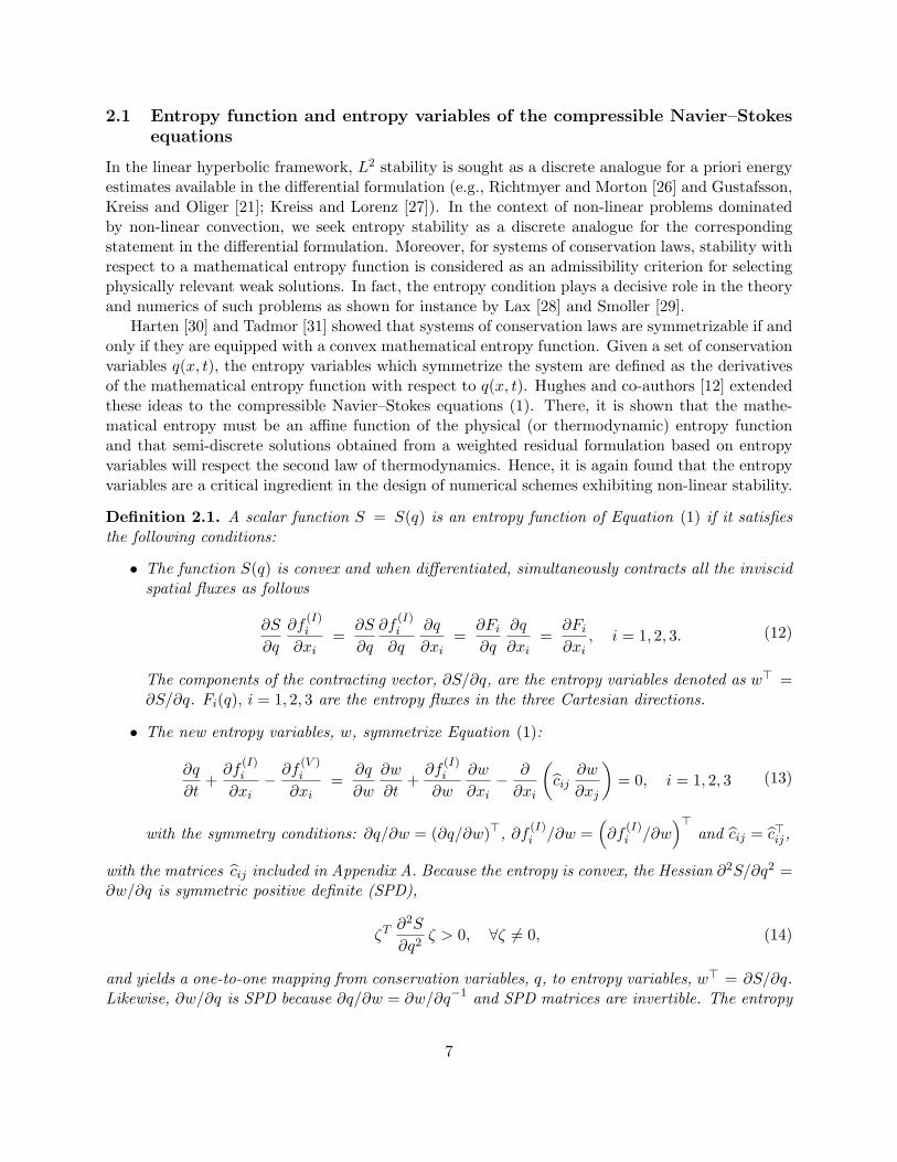
2.1 Entropy function and entropy variables of the compressible Navier–Stokesequations

In the linear hyperbolic framework, L2 stability is sought as a discrete analogue for a priori energyestimates available in the differential formulation (e.g., Richtmyer and Morton [26] and Gustafsson,Kreiss and Oliger [21]; Kreiss and Lorenz [27]). In the context of non-linear problems dominatedby non-linear convection, we seek entropy stability as a discrete analogue for the correspondingstatement in the differential formulation. Moreover, for systems of conservation laws, stability withrespect to a mathematical entropy function is considered as an admissibility criterion for selectingphysically relevant weak solutions. In fact, the entropy condition plays a decisive role in the theoryand numerics of such problems as shown for instance by Lax [28] and Smoller [29].

Harten [30] and Tadmor [31] showed that systems of conservation laws are symmetrizable if andonly if they are equipped with a convex mathematical entropy function. Given a set of conservationvariables q(x, t), the entropy variables which symmetrize the system are defined as the derivativesof the mathematical entropy function with respect to q(x, t). Hughes and co-authors [12] extendedthese ideas to the compressible Navier–Stokes equations (1). There, it is shown that the mathe-matical entropy must be an affine function of the physical (or thermodynamic) entropy functionand that semi-discrete solutions obtained from a weighted residual formulation based on entropyvariables will respect the second law of thermodynamics. Hence, it is again found that the entropyvariables are a critical ingredient in the design of numerical schemes exhibiting non-linear stability.

Definition 2.1. A scalar function S = S(q) is an entropy function of Equation (1) if it satisfiesthe following conditions:

• The function S(q) is convex and when differentiated, simultaneously contracts all the inviscidspatial fluxes as follows

∂S

∂q

∂f(I)i

∂xi=

∂S

∂q

∂f(I)i

∂q

∂q

∂xi=

∂Fi∂q

∂q

∂xi=

∂Fi∂xi

, i = 1, 2, 3. (12)

The components of the contracting vector, ∂S/∂q, are the entropy variables denoted as w> =∂S/∂q. Fi(q), i = 1, 2, 3 are the entropy fluxes in the three Cartesian directions.

• The new entropy variables, w, symmetrize Equation (1):

∂q

∂t+∂f

(I)i

∂xi−∂f

(V )i

∂xi=

∂q

∂w

∂w

∂t+∂f

(I)i

∂w

∂w

∂xi− ∂

∂xi

(cij

∂w

∂xj

)= 0, i = 1, 2, 3 (13)

with the symmetry conditions: ∂q/∂w = (∂q/∂w)>, ∂f (I)i /∂w =

(∂f

(I)i /∂w

)>and cij = c>ij,

with the matrices cij included in Appendix A. Because the entropy is convex, the Hessian ∂2S/∂q2 =∂w/∂q is symmetric positive definite (SPD),

ζT∂2S

∂q2ζ > 0, ∀ζ 6= 0, (14)

and yields a one-to-one mapping from conservation variables, q, to entropy variables, w> = ∂S/∂q.Likewise, ∂w/∂q is SPD because ∂q/∂w = ∂w/∂q−1 and SPD matrices are invertible. The entropy

7

and corresponding entropy flux are often denoted as entropy–entropy flux pair, (S, F ), [13]. If theentropy function S(q) is convex, a bound on its global estimate can be converted into an a prioriestimate on the solution of (1) in suitable Lp space [32].

The symmetry of the matrices ∂q/∂w, ∂f (I)i /∂w indicates that the conservative variables, q,

and the inviscid fluxes, f (I)i , are Jacobians of scalar functions with respect to the entropy variables,

q> =∂ϕ

∂w,(f

(I)i

)>=∂ψi∂w

, (15)

where the non-linear function, ϕ, is called the potential and ψi, i = 1, 2, 3 are called the poten-tial fluxes [13]. Just as the entropy function is convex with respect to the conservative variables(∂2S/∂q2 is SPD), the potential function is convex with respect to the entropy variables.

Godunov [33] proved that (see reference [30] for a detailed summary of the proof):

Theorem 2.1. If Equation (1) can be symmetrized by introducing new variables w, and q is aconvex function of ϕ (the so-called potential), then an entropy function S(q) is given by

ϕ = w>q − S, (16)

and the entropy fluxes satisfyψi = w>f

(I)i − Fi, (17)

where ψi, i = 1, 2, 3, are the so-called potential fluxes. The potential and the corresponding potentialflux are usually denoted as potential–potential flux pair, (ϕ,ψ), [13].

In the specific case of the compressible Navier–Stokes equations, the entropy–entropy flux pairis

S = −ρ s, Fi = −ρ ui s, i = 1, 2, 3, (18)

and the potential–potential flux pair is

ϕ = ρR, ψi = ρ uiR, i = 1, 2, 3. (19)

Note that the mathematical entropy has the opposite sign of the thermodynamic entropy. To avoidconfusion, herein entropy refers to the mathematical entropy unless otherwise noted. The entropyvariables using the pair in (18) are

w =(∂S

∂q

)>=(h

T− s− uiui

2T,u1

T,u2

T,u3

T,− 1

T

)>, (20)

and may be shown to have a one-to-one mapping with the conservative variables provided ρ, T > 0.Expressly:

ζT∂2S

∂q2ζT > 0, ∀ζ 6= 0, ρ, T > 0.

This restriction on density and temperature weakens the entropy proof, making it less than fullmeasure of non-linear stability. Another mechanism must be employed to bound ρ and T away fromzero to guarantee stability and positivity; positivity preservation will not be considered herein.

8

3 No-slip boundary conditions: Continuous analysis

The problem of well-posed boundary conditions is an essential question in many area of physics.For the two- (2D) and three-dimensional (3D) Navier–Stokes equations, the number of boundaryconditions implying well-posedness can be obtained using the Laplace transform technique [21];a complicated procedure for system of partial differential equations (PDEs) like the compressibleNavier–Stokes equations. Nordstrom and Svard [22] proposed an alternative semi-discrete approachto arrive at the number and type of boundary conditions for a general time-dependent system ofPDEs. This analysis was applied to the linearized 3D compressible Navier–Stokes equations fordifferent flow regimes and the case of the no-penetration velocity condition.

In 2008, Svard and Nordstrom [23] showed that the no-slip boundary conditions together with aboundary condition on the temperature imply stability for the 3D linearized compressible Navier-Stokes equations. Their result, can also be generalized to assess the stability of the non-linearproblem for smooth solutions as indicated in [21, 34] and the references therein. In this section weaddress the non-linear stability (entropy stability) of the viscous wall boundary conditions for the(non-linear) compressible Navier–Stokes equations given in (1).

Contracting the system of equations (1) with the entropy variables and using relations (12) and(13) results in the differential form of the entropy equation:

∂S

∂q

∂q

∂t+∂S

∂q

∂f(I)i

∂xi=∂S

∂t+∂Fi∂xi

=∂S

∂q

∂f(V )i

∂xi=

∂

∂xi

(w>f

(V )i

)−(∂w

∂xi

)>f

(V )i

=∂

∂xi

(w>f

(V )i

)−(∂w

∂xi

)>cij

∂w

∂xj.

(21)

Integrating Equation 21 over the domain yields a global conservation statement for the entropy inthe domain

d

dt

∫Ω

S dx =[w>f

(V )i − Fi

]∂Ω−∫Ω

(∂w

∂xi

)>cij

∂w

∂xjdx =

[w>f

(V )i − Fi

]∂Ω− DT, (22)

where DT is the viscous dissipation term,

DT =∫Ω

(∂w

∂xi

)>cij

∂w

∂xjdx .

It is shown in [16] that the 15× 15 matrix c (i.e., cij , 1 ≤ i, j ≤ 3) in the integral term is positivesemi-definite, which makes the term −DT strictly dissipative. Note that the entropy can onlyincrease in the domain based on data that convects and diffuses through the boundaries. The signof the entropy change due to viscous dissipation is always negative.2

To simplify, we let the domain of interest, Ω, be the unit cube 0 ≤ x1, x2, x3 ≤ 1. Expanding

2From a physical point of view, this means that the viscous dissipation always yields an increase of the thermo-dynamic entropy.

9

the Einstein notation in equation (22) yields

d

dt

∫Ω

S dx1 dx2 dx3 = −DT

+∫

x1=0

[+F1 − w>

(c11

∂w

∂x1+ c12

∂w

∂x2+ c13

∂w

∂x3

)]dx2 dx3

+∫

x1=1

[−F1 + w>

(c11

∂w

∂x1+ c12

∂w

∂x2+ c13

∂w

∂x3

)]dx2 dx3

+∫

x2=0

[+F2 − w>

(c12

∂w

∂x1+ c22

∂w

∂x2+ c23

∂w

∂x3

)]dx1 dx3

+∫

x2=1

[−F2 + w>

(c12

∂w

∂x1+ c22

∂w

∂x2+ c23

∂w

∂x3

)]dx1 dx3

+∫

x3=0

[+F3 − w>

(c13

∂w

∂x1+ c23

∂w

∂x2+ c33

∂w

∂x3

)]dx1 dx2

+∫

x3=1

[−F3 + w>

(c13

∂w

∂x1+ c23

∂w

∂x2+ c33

∂w

∂x3

)]dx1 dx2 .

(23)

Consider the case of a wall placed at x1 = 0, and assume that all the other boundaries termsare stable; their contributions are neglected without loosing generality. Therefore, estimate (23)reduces to

d

dt

∫Ω

S dx1 dx2 dx3 = −DT

+∫

x1=0

[F1 − w>

(c11

∂w

∂x1+ c12

∂w

∂x2+ c13

∂w

∂x3

)]dx2 dx3 .

(24)

To bound the time derivative of the entropy, the right-hand-side (RHS) of Equation (24) requiresboundary data. In the case of a solid viscous wall (assuming linear analysis) four independentboundary conditions must be imposed [34].3 The no-slip boundary conditions are u1 = u2 = u3 = 0(i.e., the velocity vector relative to the wall is the zero vector). For the linearized compressibleNavier–Stokes equations, the fourth condition is the gradient of the temperature normal to thewall, (∂T/∂n)wall, (Neumann boundary condition; e.g., the adiabatic wall), or the temperature ofthe wall, Twall, (the Dirichlet or isothermal wall boundary condition), or a mixture of Dirichletand Neumann conditions (the Robin boundary condition). These four boundary conditions leadto energy stability (linear stability); see, for instance, [23, 35]. In the remainder of this section, wewill show the type and the form of the wall boundary conditions that have to be imposed to boundestimate (24) and, hence, to attain entropy stability.

Consider the inviscid contribution to the boundary terms in (24).

Theorem 3.1. The no-slip boundary conditions u1 = u2 = u3 = 0 bound the inviscid contributionto the time derivative of the entropy in equation (24).

3A solid wall behaves like a subsonic outflow [22].

10

Proof. Equation (17) provides the definition of the entropy flux, F1:

F1 = w>f(I)1 − ψ1, ψ1 = ρu1R. (25)

Substituting the no-slip conditions, u1 = u2 = u3 = 0, into the definition of the inviscid flux, f (I)1 ,

(Equation 3) and the condition u1 = 0 into the definition of ψ1, yields the desired result F1 = 0.

A similar proof appears in the work of Svard and Ozcan [20], where a SAT approach on the con-servative variables is used.

Consider now the viscous contribution to the boundary terms in (24).

Theorem 3.2. The entropy flux boundary condition,

g(t) =∂T

∂n

1T, (26)

where the symbol n defines the normal direction to the wall, bounds the viscous contribution to thetime derivative of the entropy (24).

Proof. Using the definition of matrices cij given in Appendix A, the viscous vector-matrix-vectorcontraction given in (24) yields the following term

− w>(c11

∂w

∂x1+ c12

∂w

∂x2+ c13

∂w

∂x3

)= κ

(∂T

∂x1

1T

). (27)

Therefore, specifying the condition g(t) =(∂T∂x1

1T

)where g(t) is a known bounded function (i.e.,

L2 ∩ L∞), eliminates the last potential source of instability on the right-hand-side of equation(24).

The boundary condition given by Theorem 3.2 at first glance appears ad hoc. Note, however,that the scalar value κ

(∂T∂x1

1T

)accounts for the change in entropy at the boundary x1 = 0, due to

the wall heat flux, qwall, also denoted heat entropy transfer or heat entropy flow [36]. In fact,

κ∂T

∂x1

1T

= −κ ∂

∂x1[w(5)]

1w(5)

= κ∂

∂x1[log(T )] = −qwall

Twall, (28)

where w(5) represents the fifth component of the entropy variable vector, w, in (20). Equation(28) indicates that, in the context of the entropy stability analysis of the compressible Navier–Stokes equations, it is admissible and physically (thermodynamically) correct to impose the fourthwall boundary condition as given in Theorem 3.2. Such a boundary conditions can be seen as anon-linear mixed Dirichlet and Neumann boundary condition.

To the best of our knowledge, Theorem 3.2 provides new insight for future development of anyentropy stable boundary conditions for the compressible Navier–Stokes equations.

Remark 3.1. We strongly remark that the non-linear contraction obtained in (27) is differentfrom that obtained from the linearized compressible Navier–Stokes equations [23, 35]. The linearanalysis produces velocity gradient terms in the energy estimate, and temperature gradient terms inthe normal direction of the form T ∂T

∂x1, with T and ∂T

∂x1being perturbations.

Remark 3.2. The boundary condition g(t) = 0, which corresponds to an adiabatic wall ∂T/∂x1 =0, bounds the solution, and, as physically expected, does not contribute to the time derivative of theentropy (24).

11

4 Entropy stable spectral discontinuous collocation method forthe semi-discretized system: Interior operator

In this section, we summarize the main results that allow us to construct a numerical high orderentropy stable discontinuous spectral collocation interior operator of any order, p. The formalismprovided here, will then be used in Section 5 to design new entropy stable solid wall boundaryconditions for the semi-discretized compressible Navier–Stokes equations.

Using an SBP operator and its equivalent telescoping form (see Appendix B), the semi-discreteform of the compressible Navier–Stokes equations (1) becomes

∂q∂t

= Dxi

(−f (I)

i + cijDxjq)

+ P−1xi

(g(B) + g(In)) = P−1xi

∆xi

(−f

(I)i + f

(V )i

)+ P−1

xi(g(B) + g(In))

q(x, 0) = g(0)(x), x ∈ Ω.(29)

The source terms g(B) and g(In) contain the enforcement of boundary and interface conditions,respectively; and g(0) represents the initial condition. The matrix P incorporates the local gridspacing into the derivative definition, and it may be thought of as a mass matrix in the contextof Galerkin FE method. While it is not true in general that P is diagonal, herein the focus isexclusively on diagonal norm SBP operators, based on fixed element-based polynomials of orderp. The matrix D is used to approximate the first derivative; and it is defined as P−1Q, where thenearly skew-symmetric matrix, Q, is an undivided differencing operator where all rows sum to zeroand the first and last column sum to −1 and 1, respectively. The operator ∆ is the telescopic fluxmatrix and allows to express the semi-discrete system in a telescopic flux form, by evaluating thefluxes at the collocated flux points, f

(I) and f(V ),4 (see Figure 1).

x1 x2 x3 x4 x5

x0 x1 x2 x3 x4 x5

u0 u1 u2 u3 u4

f1 f2 f3 f4 f5

f0 f1 f2 f3 f4 f5

−1 −910

−√

37

−1645

0−1645

+1645

+√

37

+910

+1

Figure 1. The one-dimensional discretization for p = 4 Legendre collocation. Solution points aredenoted by • and flux points are denoted by ×.

The semi-discrete entropy estimate is achieved by mimicking term by term the continuousestimate given in Equation (21). The non-linear analysis begins by contracting the semi-discreteequations given in Equation (29), with the entropy variables: w>P. For clarity of presentation,but without loss of generality, the derivation is simplified to one spatial dimension. Tensor productalgebra allows the results to extend directly to three dimensions. The resulting global equation

4In the reminder of this work, all quantities evaluated at the flux points are denoted by an over-bar.

12

that governs the time derivative of the entropy is given by

w>P ∂q∂t

+ w>∆f(I) = w>∆f

(V ) + w>(g(B) + g(In)), (30)

wherew =

(w(q1)>, w(q2)>, . . . , w(qN )>

)>,

is the vector of entropy variables.

4.1 Time derivative

The time derivative in (30) is in mimetic form for diagonal norm SBP operators. The entropyvariables are defined by the expression w> = ∂S/∂q, which when combined with the definition ofentropy yields the point-wise expression

w>i∂qi∂t

=∂Si∂qi

∂qi∂t

=∂Si∂t

, ∀i.

Now, define the diagonal matrices ∂S/∂q = W = diag[w]. Since P is a diagonal matrix andarbitrary diagonal matrices commute, the semi-discrete rate of change of entropy becomes

w>P ∂q∂t

= 1>WP ∂q∂t

= 1>PW∂q∂t

= 1>P ∂S∂q

∂q∂t

= 1>P ∂S∂t,

where1 = (1, 1, . . . , 1)> ,

is a vector with N elements.5

4.2 Inviscid terms

The inviscid portion of Equation (30) is entropy conservative if it satisfies

w>∆f(I) = F (qN )− F (q1) = F (qN )− F (q1) = 1>∆F. (31)

Note that in (31), the first and last flux points are coincident with the first and last solutionpoints, which enables the endpoint fluxes to be consistent (see Figure 1). One plausible solutionto Equation (31) is a point-wise relation between solution and flux-point data, which telescopesacross the domain and produces the entropy fluxes at the boundaries. Tadmor [13] developed sucha solution based on second-order accurate centered operators. Carpenter and co-authors [37], havegeneralized this solution for Legendre spectral collocation operators of any order of accuracy, p.

In the following paragraphs, we present, without any proof, the main theorems which allowto construct inviscid entropy conservative and stable fluxes of any order of accuracy. Interestedreaders should consult [16, 37] and the references therein for details. Note that in this section thesubscripts i − 1, i and i + 1 are used to denote a scalar or vector quantity at the i − 1, i or i + 1collocated point, and do not have to be confused with the subscript used for instance in (1).

5N = p+ 1 for a pth-order scheme.

13

Theorem 4.1. The local conditions

(wi+1 − wi)> f i = ψi+1 − ψi, i = 1, 2, . . . , N − 1 ; ψ1 = ψ1, ψN = ψN (32)

when summed, telescope across the domain and satisfy the entropy conservative condition givenin Equation (31). A flux that satisfies this condition given in equation (32) is denoted f

(S)i . The

potentials ψi+1 and ψi need not be the point-wise ψi+1 and ψi, respectively.

A possible strategy for constructing high order entropy conservative fluxes is to construct alinear combination of two-point entropy conservative fluxes by using the coefficients in the SBPmatrix Q. This approach follows immediately from the generalized telescoping structural propertiesof diagonal norm SBP operators given in Section B.1. Because it requires only the existence ofa two-point entropy conservative flux formula and the coefficients of Q, it is valid for any SBPoperator that satisfies the constraints given in (B3). Thus, it is also valid for Legendre spectralcollocation operators used herein.

The following theorem establishes the accuracy of the new fluxes.

Theorem 4.2. [16] A two-point entropy conservative flux can be extended to high order withformal boundary closures by using the form

f(S)i =

N∑k=i+1

i∑`=1

2Q`k fS (q`, qk) , 1 ≤ i ≤ N − 1, (33)

when the two-point non-dissipative function from Tadmor [13],

fS (qk, q`) =

1∫0

g (w(qk) + ξ (w(q`)− w(qk))) dξ, g(w(u)) = f(u), (34)

is used. The coefficient, Qk`, corresponds to the k row and l column in Q.

Thus, Theorem 4.2 ensures that a high order flux constructed from a linear combination oftwo-point entropy conservative fluxes retains the design order of the original discrete operator forany diagonal norm SBP matrix Q.

The following theorem establishes instead that the linear combination of two-point entropyconservative fluxes does preserve the property of entropy stability for any arbitrary diagonal normSBP matrix Q.

Theorem 4.3. [16] A two-point high order entropy conservative flux satisfying Equation (32) withformal boundary closures can be constructed using Equation (33),

f(S)i =

N∑k=i+1

i∑`=1

2Q`k fS (q`, qk) , 1 ≤ i ≤ N − 1, (35)

where fS (q`, qk) is any two-point non-dissipative function that satisfies the entropy conservationcondition

(w` − wk)> fS (q`, qk) = ψ` − ψk. (36)

14

The high order entropy conservative flux satisfies an additional local entropy conservation property,

w>P−1∆f(S) = P−1∆F =

∂

∂xF (q) + Tp+1, (37)

where Tp+1 is the truncation error of the approximation, or equivalently,

w>i

(f

(S)i − f (S)

i−1

)=(F i − F i−1

), 1 ≤ i ≤ N, (38)

where

F i =N∑

k=i+1

i∑`=1

Q`k[(w` + wk)

> fS (q`, qk)− (ψ` + ψk)], 1 ≤ i ≤ N − 1. (39)

4.2.1 Affordable entropy consistent Euler flux

The inviscid terms in the discretization of the compressible Navier–Stokes equations (29) are cal-culated according to Equations (33) and (34) by using the two-point entropy conservative flux ofIsmail and Roe [38],

fS,j(qi, qi+1) =(ρuj , ρuj u1 + δj1p, ρuj u2 + δj2p, ρuj u3 + δj3p, ρujH

)>,

u =

ui√Ti

+ υi+1√Ti+1

1√Ti

+ 1√Ti+1

, p =

pi√Ti

+ pi+1√Ti+1

1√Ti

+ 1√Ti+1

,

h = R

log( √

Tiρi√Ti+1ρi+1

)1√Ti

+ 1√Ti+1

(θ1 + θ2) ,

θ1 =√Tiρi +

√Ti+1ρi+1(

1√Ti

+ 1√Ti+1

)(√Tiρi −

√Ti+1ρi+1

) ,

θ2 =γ + 1γ − 1

log(√

Ti+1

Ti

)log(√

TiTi+1

ρi

ρi+1

)(1√Ti− 1√

Ti+1

) ,

H = h+12u`u`, ρ =

(1√Ti

+ 1√Ti+1

)(√Tiρi −

√Ti+1ρi+1

)2(log(√Tiρi)− log(

√Ti+1ρi+1)

) .

(40)

The index j denotes the spatial direction. This somewhat complicated explicit form is the firstentropy conservative flux for the convective terms with low enough computational cost to be im-plemented in a practical simulation code.

4.2.2 Entropy stable inviscid interface flux

Herein, the solution between adjoining elements is allowed to be discontinuous. An interface fluxthat preserves the entropy consistency of the interior operators on either side of the interface is

15

needed. An entropy consistent (or entropy conservative) inviscid interface flux constructed accord-ing to equations (33) and (34) by using (40) is indicated as f sr

(q

(−)i , q

(+)i

). A more dissipative and

hence stable entropy inviscid interface flux f ssr(q

(−)i , q

(+)i

)is constructed as

f ssr(q

(−)i , q

(+)i

)= f sr

(q

(−)i , q

(+)i

)+ Λ

(w

(+)i − w(−)

i

), (41)

where Λ is a negative semi-definite interface matrix with zero or negative eigenvalues. The entropystable flux f ssr

(q

(−)i , q

(+)i

)is more dissipative than the entropy conservative inviscid flux, as is

easily verified by contracting f ssr(q

(−)i , q

(+)i

)against the entropy variables to yield the expression(

w(+)i − w(−)

i

)>f ssr

(q

(−)i , q

(+)i

)= ψ

(+)i − ψ(−)

i +(w

(+)i − w(−)

i

)>Λ(w

(+)i − w(−)

i

). (42)

The superscripts (−) and (+) combined with the subscript i denote the left and right state used tocompute the two-point entropy conservative flux and therefore replace the subscripts i and i+ 1 in(40). The matrix Λ can be constructed using different approaches, e.g., using an upwind operatorthat dissipates each characteristic wave based on the magnitude of its eigenvalue:

f ssc(q

(−)i , q

(+)i

)= f sr

(q

(−)i , q

(+)i

)+ 1/2Y |λ| Y>

(w

(−)i − w(+)

i

),

∂

∂qf (q) = Y λY>,

∂q

∂w= YY>,

(43)

where λ and Y are the diagonal matrix of the eigenvalues and the matrix of the eigenvectors,respectively. Note that the relation ∂q

∂w = YYT is achieved by an appropriate scaling of therotation eigenvectors. See the work of Merriam [39] for more details. Unless otherwise noted, theentropy stable characteristic flux is used in all test simulations presented herein.

4.3 Viscous Terms

Using the SBP formalism (see Appendix B.2), the contribution of the viscous terms to the semi-discrete time derivative of the entropy is

w>∆f(V ) = w>B c11Dw − (Dw)> P c11 (Dw) . (44)

The last term is negative semi-definite. As with the continuous estimate given in (23), only theboundary term can produce a growth of the entropy, and thus the approximation of the viscousterms is entropy stable. (Entropy stable boundary conditions bound these terms.)

5 Entropy stable solid wall boundary conditions for the semi-discrete system

An estimate for the time derivative of the entropy of a isolated element is derived, followed by aderivation of entropy stable penalty terms that imposed physical data on the boundaries.6

6The same boundary conditions (without stability proofs) could be used for almost any spatial discretizationincluding the family of DG methods, FR approaches, WENO schemes, FD and FV methods.

16

5.1 General approach for the entropy stability analysis of a SBP-based spatialdiscretization

Consider a single tensor product element and a spatially discontinuous collocation discretizationwith N = p + 1 solution points in each coordinate direction; the following element-wise matriceswill be used:

Dx1 = (DN ⊗ IN ⊗ IN ⊗ I5) , Dx2 = (IN ⊗DN ⊗ IN ⊗ I5) ,Dx3 = (IN ⊗ IN ⊗DN ⊗ I5) ,

∆x1 = (∆N ⊗ IN ⊗ IN ⊗ I5) , ∆x2 = (IN ⊗∆N ⊗ IN ⊗ I5) ,∆x3 = (IN ⊗ IN ⊗∆N ⊗ I5) ,

Px1 = (PN ⊗ IN ⊗ IN ⊗ I5) , Px2 = (IN ⊗ PN ⊗ IN ⊗ I5) ,Px3 = (IN ⊗ IN ⊗ PN ⊗ I5) , Px1x2 = (PN ⊗ PN ⊗ IN ⊗ I5) ,Px1x3 = (PN ⊗ IN ⊗ PN ⊗ I5) , Px2x3 = (IN ⊗ PN ⊗ PN ⊗ I5) ,

P = Px1x2x3 = (PN ⊗ PN ⊗ PN ⊗ I5) ,

Bx1 = (BN ⊗ IN ⊗ IN ⊗ I5) , Bx2 = (IN ⊗ BN ⊗ IN ⊗ I5) ,Bx3 = (IN ⊗ IN ⊗ BN ⊗ I5) ,

(45)

where DN , PN , ∆N , and BN are the one-dimensional (1D) SBP operators [40], and IN is the identitymatrix of dimension N . I5 denotes the identity matrix of dimension five.7 The subscripts in (45)indicate the coordinate directions to which the operators apply (e.g., Dx1 is the differentiationmatrix in the x1 direction). Furthermore, we define the norm w>Pq = ‖S‖2P , where w and Sare the vector of the entropy variables at the solution points and the mathematical entropy of thesystem, respectively. When applying these operators to the scalar entropy equation in space, a hatwill be used to differentiate the scalar operator from the full vector operator. For example,

P = (PN ⊗ PN ⊗ PN ) . (46)

Within one tensor product element, the 3D compressible Navier–Stokes equations are discretizedas

∂q∂t

+ P−1x1

∆x1

(f

(I)1 − f

(V )1

)+ P−1

x2∆x2

(f

(I)2 − f

(V )2

)+ P−1

x3∆x3

(f

(I)3 − f

(V )3

)= P−1

x1

(g(B)

1 + g(In)1

)+ P−1

x2

(g(B)

2 + g(In)2

)+ P−1

x3

(g(B)

3 + g(In)3

),

(47)

where the vector of conservative variables is ordered as

q =(q(x(1)(1)(1)

)>, q(x(1)(1)(2)

)>, . . . , q

(x(N)(N)(N)

)>) =(q(1)>, q(2)

>, . . . , q(N3)>), (48)

and f(I)i and f

(V )i are the grid fluxes.8 The vector g(B)

i , i = 1, 2, 3 enforces the boundary conditions,while g(In)

i i = 1, 2, 3 patches interfaces together. The derivatives appearing in the viscous fluxes

f(V )i are also computed using the operator Dxi , i = 1, 2, 3 from expression (45).

7The 3D compressible Navier–Stokes equations form a system of five non-linear PDEs.8Recall that the vectors with an over-bar are defined at the flux points.

17

As in the continuous case, we apply the entropy analysis to Equation (47) by multiplyingwith w>P from the left. Moreover, we substitute to f

(I)i , i = 1, 2, 3 the high-order accurate

entropy consistent flux constructed according to Equations (33) and (34) with the two-point entropyconservative flux presented in Section 4.2.1. The final expression for the time derivative of theentropy in the element is then

d

dt‖S‖2P + 1>

(Px2x3Bx1F1 + Px1x3Bx2F2 + Px1x2Bx3F3

)− w>

(Px2x3Bx1f

(V )1 + Px1x3Bx2f

(V )2 + Px1x2Bx3f

(V )3

)+ DT

= w>(Px2x3

(g(B)

1 + g(In)1

)+ Px1x3

(g(B)

2 + g(In)2

)+ Px1x2

(g(B)

3 + g(In)3

)).

(49)

Note that in (49) the bar over the flux vectors could be safely removed because the contraction of(47) against w>P leads only to the boundary fluxes, which satisfy the duality condition (B12) (seeFigure 1). The quantity DT denotes a positive quadratic term in the first derivative approximationof the solution:

DT =3∑i=1

3∑j=1

(Dxiw)>P [cij ](Dxjw

)

=

Dx1 wDx2 wDx3 w

>P [c11] P [c12] P [c13]P [c21] P [c22] P [c23]P [c31] P [c32] P [c33]

Dx1 wDx2 wDx3 w

,

(50)

where [cij ] denotes a block diagonal matrix with blocks corresponding to the viscous coefficients ofeach solution point. The positive semi-definiteness of DT follows from the positivity of the matricescij used to define [cij ] (see Appendix B.2 in [16] for the proof). The matrices Bxi , i = 1, 2, 3 pickthe interface terms in the respective directions (i.e., for a high-order accurate scheme on a tensorproduct cell, they pick the solution value at the nodes of the two “opposite” faces). Therefore,Equation (49) is the semi-discrete form of Equation (23), which was obtained from the analysis atthe continuous level.

5.2 Entropy stability analysis for the solid wall boundary conditions

We focus now on the construction of an entropy stable penalty term for imposing the solid wallboundary conditions for the compressible Navier–Stokes equations. The boundary conditions thatare developed herein are motivated by the general interface coupling conditions used to cou-ple elements in the interior of the domain. The interior conditions combine an entropy stablecharacteristic-based coupling condition for the inviscid terms, with a local discontinuous Galerkin(LDG) approach and interior penalty (IP) procedure of the viscous terms. Details of the interiorcoupling terms can be found in Appendix C. These interface terms include a refinement of the IPcoupling terms relative to those presented elsewhere [41].

Without loss of generality, we study a hexahedral element with edge length equal to one andwe consider only the face plane (0, x2, x3). With these assumptions, Equation (49) reduces to

d

dt‖S‖2P − 1>Px2x3 G(1)F1 + w>Px2x3G(1)f

(V )1 + DT = w>Px2x3G(1)g

(B)1 . (51)

18

The operators G(k) and G(k) are defined as

G(k) = (ek ⊗ IN ⊗ IN ) , G(k) = (ek ⊗ IN ⊗ IN ⊗ I5) , (52)

whereek = (0, 0, . . . , 1, 0, . . . , 0, 0)>

is a vector of length N and has a non-zero element corresponding to the solution location, k.Therefore, the operators G(k) and G(k) pick out the nodal values of the solution or any flux vectorat a specific plane according to the ordering introduced in (48). Herein, the face plane (0, x2, x3)is characterized by the index k = 1. Thus, Equation (51) represents the contribution to the timederivative of the entropy of the boundary points that lie on the face plane (0, x2, x3).

In the remainder of this paper, we assume that the node with solution vector q(x(1)(1)(1)

)= q(1)

(see expression (48)) lies on this face plane. This point will be used to derive the entropy stablewall boundary conditions. All numerical states associated to it will be identified with the subscript(·)(1).

The penalty source term g(B)1 is composed of three design-order terms that weakly enforce the

boundary conditions:

g(B)1 = −

(f

(I)1 (q)− f sr1

(q,g(E)

))+(f

(V )1 − f

(V,B)1

)+ [M ]

(w − g(NS),V el

). (53)

In each of the three contributions, the first component (the numerical state) is constructed fromthe numerical solution, while the second component (the boundary state) is constructed from acombination of the numerical solution and four independent components of physical boundarydata.

The first term enforces the no-penetration Euler wall condition through the inviscid flux of thecompressible Euler equations. The boundary state is formed by constructing an entropy conserva-tive flux based on the numerical state q(1) and a manufactured boundary state given by the vectorg(E):

g(E) =

1 0 0 0 00 −1 0 0 00 0 1 0 00 0 0 1 00 0 0 0 1

q>(1) =(ρ(1),− (ρu1)(1) , (ρu2)(1) , (ρu3)(1) , (ρE)(1)

)>. (54)

The second term enforces the thermal boundary condition (26), facilitated by manufacturinga boundary viscous flux f

(V,B)1 . Define the component of the gradient of the entropy variables in

the numerical state as Θx1 , Θx2 and Θx3 . Next, specify the value of the heat entropy flux g(t), theexternally provided bounded function defined as in (26). Finally, define Θx1 as

Θx1 = [Θx1(1),Θx1(2),Θx1(3),Θx1(4), Θx1(5)]>,

where Θx1(5) is computed as

Θx1(5) = −g(t)w(1)(5) =g(t)T(1)

. (55)

19

With these definitions, the manufactured viscous flux f (V,B)1 is constructed as

f(V,B)1 = c11Θx1 + c12Θx2 + c13Θx3 , (56)

where c1j , j = 1, 2, 3, is constructed from the numerical state. Note that for an adiabatic wallg(t) = 0, and from expression (55) we get Θx1(5) = 0.

The third term in (53) enforces the no-slip wall Dirichlet boundary conditions (u1 = u2 = u3 =0) through a standard SAT approach. The manufactured boundary state g(NS),V el is defined interms of entropy variables as

g(NS),V el =(w(1)(1), 0, 0, 0, w(1)(5)

)>, (57)

where w(1)(1) and w(1)(5) are the first and the fifth components of the entropy vector constructedfrom the numerical state. Three boundary conditions are imposed in Equation (57); all velocitycomponents are set to zero at the wall. This is immediately clear by recalling that the entropyvariables for the compressible Navier–Stokes equations are defined as

w =(h

T− s− uiui

2T,u1

T,u2

T,u3

T,− 1

T

)>.

The matrix [M ] is a block diagonal matrix whose five-by-five blocks are defined as

M = − α(B)

(Px1)(1)(1)

H c11H, H = diag(1, 1, 1, 1, 0). (58)

The matrix c11 has the functional form of the usual symmetric positive semi-definite matrix c11

defined in Appendix A. This matrix has to be constructed using a set of primitive variables thatis independent of the numerical solution at all times. For instance, for external flows, c11 can beconstructed using the externally provided data at the far-field (e.g., (ρ∞, |~u∞|, |~u∞|, |~u∞|, T∞)).9

The coefficient α(B) is a positive value used to modify the strength of the SAT penalty term, andcan be specified by the user. The factor (Px1)(1)(1) in the denominator is introduced to achievethe correct asymptotic order of accuracy; it allows an increase in the strength of M with increasedresolution in the normal direction.

Summarizing Equation (53), the penalty at the face point is the sum of three terms:

• the difference between inviscid flux and the entropy consistent flux at the node in the normaldirection;

• the difference between the internal viscous flux and a boundary viscous flux at the node inthe normal direction;

• the difference between the solution (in entropy variables) at the node and the data imposedat boundary, multiplied by the matrix M .

9In a general framework, the matrix M is built using the five-by-five matrix ecii where the index i denotes thenormal direction to the wall.

20

The penalty term (53) contracted with the entropy variables and simplified, yields the expression

RHS =−w>Px2x3G(1)

(f

(I)1 (q)− f sr1

(q,g(E)

))+ w>Px2x3G(1)

(f

(V )1 − f

(V,B)1

)+ w>Px2x3G(1)[M ]

(w − g(NS),V el

).

(59)

The entropy stability of the penalty source term (51) defined by Equation (53) is demonstratedin the following theorems. First, the inviscid term is proven to be entropy conservative and thenentropy stable, if dissipation is added. Next, the second term, which specifies the thermal condition,is proven to be bounded by physical data provided by the user. Finally, the third term, whichspecifies the no-slip boundary conditions, is proven to be entropy stable.

Theorem 5.1. The penalty inviscid flux contribution in Equation (53) is entropy conservative ifthe vector g(E) is defined as in (54).

Proof. The inviscid contribution, Υ(I), to the time derivative of the entropy can be written as (seeEquations (51) and (59))

Υ(I) = (Px2x3)(1)(1) F 1 − w>1 (Px2x3)(1)(1)

[f1

(q(1)

)− fsr1

(q(1), g

(E))], (60)

where w(1) denotes again the entropy variables at the boundary face point and (Px2x3)(1)(1) 6= 0.Substituting the expression for the entropy flux F 1 (i.e., Equation (17) with i = 1) and evaluatingthe entropy consistent flux fsr1 using q(1) and g(E) yields the desired result

Υ(I) = (Px2x3)(1)(1)

[w>(1)f

(I)1

(q(1)

)− ψ1 − w>(1)f

(I)1 (q1) + w>(1)f

sr1

(q(1), g

(E))]

= (Px2x3)(1)(1)

[−ψ1 + w>(1)f

sr1

(q(1), g

(E))]

= 0.(61)

Corollary 5.1. The penalty inviscid flux contribution in Equation (53) is entropy stable if thevector g(E) is defined as in (54) and f sr is replaced by the entropy stable flux f ssr defined in (43).

Remark 5.1. A result similar to Corollary 5.1 is given by Svard and Ozcan [20] in the context ofhigh order finite differences approach.

Using Theorem 5.1 we are left only with the viscous contributions:

d

dt‖S‖2P + w>Px2x3G(1)f

(V )1 + DT ≤+ w>Px2x3G(1)

(f

(V )1 − f

(V,B)1

)+ w>Px2x3G(1)[M ]

(w − g(NS),V el

).

(62)

Theorem 5.2. The viscous penalty terms in (53)

G(1)

(f

(V )1 − f

(V,B)1

)+ G(1)[M ]

(w − g(NS),V el

)are entropy stable for any value of g(t) and any matrix M as defined in (58).

21

Proof. Clearly, the viscous flux term on the left-hand-side (LHS) of (62) is balanced by the sameterm on the RHS. Therefore, expression (62) reduces to

d

dt‖S‖2P + DT ≤−w>Px2x3G(1)f

(V,B)1 + w>Px2x3G(1)[M ]

(w − g(NS),V el

). (63)

The contraction −w>Px2x3G(1)f(V,B)1 with f

(V,B)1 defined as in (56) yields the following point-wise

contribution to the time derivative of the entropy

− w>(1) (Px2x3)(1)(1) f(V,B)1 = (Px2x3)(1)(1) κ g(t), (64)

when enforcing the heat entropy flow condition (26) through (55). Since g(t) is a known boundedfunction (i.e., L2 ∩ L∞) expression (64) is also bounded. We highlight that for an adiabatic wallg(t) = 0 and consequently the viscous flux penalty in (53) conserves the entropy (as it should)because the heat flux is zero. Note that the term (64) mimics exactly the boundary contributionthat has been obtained from the continuous analysis (see Equation (27)).

We are then left with the contribution w>G(1)[M ](w − g(NS),V el

). At the nodal level, this term

can be re-written as

12

[w>(1) (Px2x3)(1)(1)Mw(1)

]− 1

2

[(g(NS),V el

)>(Px2x3)(1)(1)M g(NS),V el

]+

12

[(w(1) − g(NS),V el

)>(Px2x3)(1)(1)M

(w(1) − g(NS),V el

)].

(65)

The penalty contribution given by Equation (65), imposes the no-slip Dirichlet boundary conditionson the velocity components, and is bounded if

• M is negative definite;

• M is independent of the numerical state.

If these two conditions are fulfilled, the first and the last term in (65) introduce only dissipation,whereas the second one is a bounded term because it is just a function of data, and in general it iszero for the no-slip boundary conditions.

For a Reynolds number Re that approaches ∞, we would like to smoothly recover only theno-penetration (or wall slip) boundary condition that characterizes the Euler equations (first con-tribution in (53)). To achieve that, the five-by-five matrix M needs to be a function of Re and canbe constructed as in (58), i.e.,

M = − α(B)

(Px1)(1)(1)

H c11H, H = diag(1, 1, 1, 1, 0), α(B) > 0.

Recall that c11 has the functional form of the usual c11 matrix and it is constructed using a statethat is independent of the numerical solution.

22

6 Numerical results

The objective of this section is to demonstrate the accuracy and robustness of the new entropy stablewall boundary conditions coupled with the family of high-order entropy stable interior operatorsdeveloped in [37]. However, before proceeding with the numerical tests, we demonstrate withan example how the application of the standard procedure, which is generally used to imposedweakly the solid wall boundary conditions for the linearized Navier–Stokes equations [23], yieldsnon-entropy stable boundary treatment.

6.1 Non-entropy stable no-slip wall boundary condition: Isothermal wall

In Section 5.2, we have shown that constructing g(B)1 as in (53) yields entropy stable wall boundary

conditions. However, one might attempt to construct g(B)1 as the sum of an inviscid penalty flux

and only a viscous interior penalty term,

g(B)1 =− G(1)

[f

(I)1 (q)− f sr1

(q,g(E)

)]+ G(1) [L]

(w − g(NS)

). (66)

For an isothermal wall, for instance, g(NS) is a vector of data that imposes both the no-slip boundarycondition on the velocity vector (i.e., u1 = u2 = u3 = 0) and the wall temperature:

g(NS) =(w(1)(1), 0, 0, 0,− 1

Twall

)>. (67)

The matrix [L] in (66) is a block diagonal matrix with blocks of size five-by-five. Comparing thetwo definitions of g(B)

1 given in Equations (53) and (66), it can be shown that in the latter approachno viscous flux penalty terms are introduced. This is a key difference, and as shown in AppendixD, yields non-entropy stable solid wall boundary conditions that are highly unstable when used incombination with fine grids and/or high-order accurate polynomial representations of the solution.

6.2 Computation of a square cylinder in subsonic flow

The flow past a square cylinder represents a benchmark test case for external flow past bluffbodies. This flow has been the subject of intense experimental and numerical research in the past.In fact, this bluff body is a simple but a central shape for many engineering applications, includingaeroacoustics and air pollutant transport and dispersion in urban environments.

The flow is described in a Cartesian coordinate system (x1, x2, x3), in which the x1-axis isaligned with the inlet flow direction, the x3-axis is parallel with the cylinder axis and the x2-axisis perpendicular to both directions (see Figure 2). A fixed two-dimensional square cylinder witha side d is exposed to a uniform freestream velocity vector with modulus u∞. The length of thesquare cylinder in the x3-direction is 10 d.

The following boundary conditions are used. A uniform flow is prescribed at the inlet whichis located 10 d units upstream of the cylinder. At the outlet, located 20 d unit downstream of thecylinder, farfield boundary conditions are used. A no-penetration (Euler) boundary condition isprescribed at the upper and lower boundaries. No-slip and adiabatic conditions are enforced atthe body surface. A periodic boundary condition is used in the spanwise direction x3. In the

23

x2-direction, the solid blockage of the confined flow (i.e., the vertical distance between the upperand the lower inviscid walls) is set to 18 d.

The flow has a freestream Mach number of M∞ = 0.1, and a Reynolds number of Re∞ = 2×102.The Reynolds number is based on the modulus of the freestream velocity vector u∞ and the heightof the cylinder d. At this Reynolds number, the regime is laminar and it usually persists up toa Reynolds number of about 4 × 102. Moreover, the vortex shedding is characterized by one verywell-defined frequency [42]. A very small time step is used to integrate the system of ordinarydifferential equations (ODEs) so that the temporal error is negligible compared to that of thespatial discretization.

6.2.1 Accuracy of the no-slip wall boundary conditions

The proposed entropy stable no-slip wall boundary conditions do not force the numerical solutionto exactly fulfill the boundary conditions. Instead the effect can be described as a rubber-bandpulling the solution towards the boundary conditions. The computed boundary value (or numericalstate) typically deviates slightly from the prescribed value but the deviation is reduced as the gridis refined. Therefore, the error at the boundary can serve as a rough measure of the error of theentire solution.

We compute the maximum norm L∞ of the error of the three velocity components u1 , u2 andu3 on the complete surface of the cylinder at t = 1, for three different grids. The meshes are fullyunstructured, although a structured subdivision is used around the square cylinder and the nearwake region to perform a grid convergence study (see Figure 2). Grid 3 has 20 points on each sideof the square, 20 points in the “radial” direction in structured portion near the body, 40 points inthe near wake region in the freestream direction, and 8 points in the spanwise direction. Grid 2 andGrid 1 are obtained by taking every other and every fourth grid point of Grid 3 in the structuredregion. The simulations are performed using different orders of the polynomial (p = 1, 2, 3, 4). Theresults are shown in Tables 1, 2 and 3.

X

Y

Z X

Y

Z

Figure 2. Example of structured/unstructured grids use for the flow past a 3D square cylinder atRe∞ = 2× 102 and M∞ = 0.1.

We highlight a few observations. First, in all cases an increase in theoretical order of accuracy

24

results in a error reduction on all grids. Secondly, although the convergence rates in model problemsare shown on much finer meshes, the computed order of accuracy is very close to the formal valuebetween the medium and fine grids, even for these more realistic meshes.

Table 1 L∞ error norm of the velocity component u1 at the wall and convergence rates; t = 1; 3Dunsteady laminar flow past a square cylinder at Re∞ = 2× 102 and M∞ = 0.1.

p = 1 rate p = 2 rate p = 3 rate p = 4 rateGrid 1 4.73e-2 - 2.15e-2 - 9.61e-3 - 4.54e-3 -Grid 2 1.47e-2 1.69 2.88e-3 2.90 5.83e-4 4.04 1.39e-4 5.02Grid 3 3.55e-3 2.04 3.66e-4 2.98 3.40e-5 4.10 4.52e-6 4.94





6.2.2 Vortex shedding

In this section we investigate the vortex shedding and the time variation of the lift and dragcoefficients. We compare our results against the data reported by Sohankar et al. [43]. We computethe following quantities: The Strouhal number, f d/u∞, where f is the frequency of the vortexshedding; the time-averaged drag coefficient, cD, and the root-mean-square (RMS) of the spanwise-averaged lift coefficient, cRMS

L . We use the same grids presented in the previous section, anddifferent orders of the polynomial (p = 1, 2, 3, 4). The results are illustrated in Tables 4, 5, 6. Fromthese tables, it can be seen that in all cases the accuracy of the results improve by increasing theorder of accuracy of the scheme. We also note that, on Grid 3, which is very coarse comparedto the typical grids used with second-order FV and FD schemes, fourth- (p = 3) and fifth-order(p = 4) accurate entropy stable schemes perform very well. In fact, the aerodynamic coefficientscomputed with these two discretizations are in very good agreement with the results reported inliterature [43].

25

Table 4 Strouhal number, mean drag coefficient and spanwise-averaged RMS of the lift coefficientfor the 3D unsteady laminar flow past a square cylinder at Re∞ = 2× 102 and M∞ = 0.1; Grid 1.

Solution St 〈cD〉 cRMSL

SSDC p = 1 0.098 1.01 0.02SSDC p = 2 0.109 1.08 0.06SSDC p = 3 0.142 1.19 0.11SSDC p = 4 0.151 1.28 0.15

Sohankar et al. [43] 0.160 1.41 0.22




Sohankar et al. [43] 0.160 1.41 0.22




Sohankar et al. [43] 0.160 1.41 0.22

26

6.3 Computation of a square cylinder in supersonic free stream

The development of a high-order accurate entropy stable discretization aims to provide the nextgeneration of robust high fidelity numerical solvers for complex fluid flow simulations, for whichstandard suboptimal algorithms suffer greatly or fail completely. By computing the flow past a 3Dsquare cylinder at Re∞ = 104 and M∞ = 1.5, we provide numerical evidence of such robustness forthe complete entropy stable high order spatial discretization. This supersonic flow is characterizedby a very large range of length scales, strong shocks and expansion regions that interact with eachother, leading to complex flow patterns. During the past three decades, this fluid flow problem hasbeen thoroughly investigated by several researchers for aerodynamic applications (see for instance[44–46]).

The domain of interest spans one square cylinder edge in the x3 direction, and at the twoplanes perpendicular to this coordinate direction, periodic boundary conditions are used. Theflow is computed using an unstructured grids with 43, 936 hexahedrons. A fourth-order accurate(p = 3) entropy stable discretization without any stabilization technique is used. The body surfaceis considered adiabatic. The solution is initialized using a uniform flow at M∞ = 1.5 with zeroangle of attack.

At the beginning of the simulation a strong shock is formed in front of the blunt body. Subse-quently, the discontinuity moves upstream until it reaches a stationary position that is about 2.15square cylinder edges far from the frontal surface of the body. During this phase, additional weakershocks, which originate from the four sharp corners of the blunt body, interact with the subsonicregions formed near the walls. This complicated flow pattern, yields the formation of shock-lets inthe wake of the square cylinder. Figure 3 shows the high order grid near the blunt body and theMach number and density contours at t = 1.5. It can be seen that relatively small oscillations aregenerated in front of the shock. This numerical feature is absolutely natural and expected becausethe solution has been computed with a fourth-order accurate scheme without artificial dissipationor filtering technique. Nevertheless, the simulation remains stable at all time, and the oscillationsare always confined in small regions close to the discontinuities.

In Figures 4 a global view of the high order grid, the Mach number, density, temperature andentropy contours at t = 100 are shown. At t = 100, the shock has already reached a stationaryposition, and the flow past the square cylinder is completely unsteady, characterized by subsonicand supersonic regions. The formation of shock-lets in the near wake region are clearly visible.

7 Conclusions

Herein, we have shown that a no-slip boundary condition together with a boundary condition on theheat entropy flow, (1/T ∂T/∂n)wall, imply stability for the continuous compressible Navier–Stokesequations. The boundary condition on the heat entropy flow is in complete agreement with thethermodynamic (entropy) analysis of a generic system. An entropy stable numerical procedure ispresented for weakly enforcing these solid wall boundary conditions via a penalty approach. Theresulting semi-discrete operator mimics exactly the behavior at the continuous level. The proposednon-linear boundary treatment provides one of the most important missing information for com-pleting the non-linear stability in the L2 norm of the continuous and semi-discretized compressibleNavier–Stokes equations. Although discontinuous spectral collocation operators are used in thiswork, the new boundary conditions are compatible with any diagonal norm summation-by-parts

27

(a) High order grid in the near-body and near-wake.

1

2

3

Mach

0

3.74

(b) Mach number; ∆M = 0.0146.

1

2

Density

0.0611

2.98

(c) Density; ∆ρ = 0.0114.

Figure 3. Unsteady flow past a 3D square cylinder at Re∞ = 104 and M∞ = 1.5, computed withthe fourth-order (p = 3) accurate entropy stable spatial discretization; t = 1.5.

28

(a) High order grid.

1 2Mach

0 2.42

(b) Mach number; ∆M = 0.0095.

0.4 0.8 1.2 1.6 2Density

0.0561 2.36

(c) Density; ∆ρ = 0.0090.

29

0.8 1.2 1.6 2 2.4

Temperature

0.667 2.63

(d) Temperature; ∆T = 0.0077.

0 0.2 0.4 0.6 0.8

Entropy

-0.141 0.982

(e) Entropy; ∆s = 0.0044.

Figure 4. Unsteady flow past a 3D square cylinder at Re∞ = 104 and M∞ = 1.5, computed withthe fourth-order (p = 3) accurate entropy stable spatial discretization; t = 100.

30

spatial operator, including finite element, finite volume, finite difference, discontinuous Galerkin,and flux reconstruction schemes.

Numerical computations around a three-dimensional square cylinder in the subsonic regime areperformed to highlight the accuracy and robustness of the proposed numerical procedure. Mea-surement of forces on the cylinder showed very good agreement with the results available from theliterature. Furthermore, we have shown that wall penetration velocity (admissible in a penaltytechnique) approaches zero to design-order.

The robustness of the complete semi-discrete operator (i.e., the entropy stable interior operatorcoupled with new boundary conditions) has been demonstrated for the supersonic flow past a three-dimensional square cylinder at Re∞ = 104 and M∞ = 1.5. This test has been successfully computedwith a fourth-order accurate method without the need to introduce artificial dissipation, limitingtechniques or filtering, for stabilizing the computations, a feat unattainable with several alternativeapproaches to wall boundary conditions and high order interior operators based on linear analysis.

This work clearly indicates that, although incremental improvements to existing algorithmswill continue to improve overall capabilities, the development of novel robust numerical techniquessuch as entropy preserving or entropy stable schemes and their extension to complex problems ofindustrial relevance offers the possibility of radical advances in this area in terms of robustness,fidelity and efficiency.

References

1. Dongarra, J.; Hittinger, J.; Bell, J.; Chacon, L.; Falgout, R.; Heroux, M.; Hovland, P.; Ng,E.; Webster, C.; and Wild, S.: Applied mathematics research for exascale computing. U.S.Department of Energy, 2014.

2. Wang, Z.; Fidkowski, K.; Abgrall, R.; Bassi, F.; Caraeni, D.; Cary, A.; Deconinck, H.; Hart-mann, R.; Hillewaert, K.; Huynh, H.; Kroll, N.; May, G.; Persson, P.-O.; van Leer, B.; andVisbal, M.: High-order CFD methods: Current status and perspective. International Journalfor Numerical Methods in Fluids, vol. 72, no. 8, 2013, pp. 811–845.

3. Parsani, M.; Ghorbaniasl, G.; Lacor, C.; and Turkel, E.: An implicit high-order spectraldifference approach for large eddy simulation. Journal of Computational Physics, vol. 229,no. 14, 2010, pp. 5373–5393.

4. Persson, P.-O.: High-order LES simulations using implicit-explicit Runge–Kutta schemes. 49thAIAA Aerospace Sciences Meeting including the New Horizons Forum and Aerospace Exposi-tion, AIAA 2011-684, 2011.

5. Hartmann, R.; Held, J.; and Leicht, T.: Adjoint-based error estimation and adaptive meshrefinement for the RANS and κ − ω turbulence model equations. Journal of ComputationalPhysics, vol. 230, no. 11, 2011, pp. 4268–4284.

6. Burgess, N. K.; and Mavriplis, D. J.: High-order discontinuous Galerkin methods for turbulenthigh-lift flows. Seventh International Conference on Computational Fluid Dynamics (ICCFD7),ICCFD7-4202, 2012.

31

7. Lodato, G.; Castonguay, P.; and Jameson, A.: Discrete filter operators for large-eddy simulationusing high-order spectral difference methods. International Journal for Numerical Methods inFluids, vol. 72, no. 2, 2013, pp. 231–258.

8. Parsani, M.; Bilka, M.; and Lacor, C.: Large eddy simulation of a muffler with the high-orderspectral difference method. Spectral and high order methods for partial differential equations -ICOSAHOM 2012 , M. Azaez, H. El Fekih, and J. S. Hesthaven, eds., Springer InternationalPublishing, vol. 95 of Lecture Notes in Computational Science and Engineering , 2014, pp.337–347.

9. Bassi, F.; Botti, L.; Colombo, A.; Ghidoni, A.; and Rebay, S.: Implementation of an ExplicitAlgebraic Reynolds Stress Model in an Implicit Very High-Order Discontinuous Galerkin Solver.Spectral and high order methods for partial differential equations - ICOSAHOM 2012 , M. Azaez,H. El Fekih, and J. S. Hesthaven, eds., Springer International Publishing, vol. 95 of LectureNotes in Computational Science and Engineering , 2014, pp. 111–123.

10. Hesthaven, J. S.; and Warburton, T.: Nodal discontinuous Galerkin methods: Algorithms,analysis, and applications. Springer Publishing Company, Incorporated, 1st ed., 2007.

11. Zhu, J.; Zhong, X.; Shu, C.-W.; and Qiu, J.: Runge–Kutta discontinuous Galerkin methodusing a new type of WENO limiters on unstructured meshes. Journal of Computational Physics,vol. 248, 2013, pp. 200–220.

12. Hughes, T.; Franca, L.; and Mallet, M.: A new finite element formulation for computationalfluid dynamics: Symmetric forms of the compressible Euler and Navier–Stokes equations andthe second law of thermodynamics. Computer Methods in Applied Mechanics and Engineering ,vol. 54, no. 2, 1986, pp. 223–234.

13. Tadmor, E.: Entropy stability theory for difference approximations of nonlinear conservationlaws and related time-dependent problems. Acta Numerica, vol. 12, 2003, pp. 451–512.

14. Tadmor, E.: The numerical viscosity of entropy stable schemes for systems of conservationlaws. I. Mathematics of Computation, vol. 49, no. 179, 1987, pp. 91–103.

15. Fisher, T. C.; and Carpenter, M. H.: High-order entropy stable finite difference schemes fornonlinear conservation laws: Finite domains. NASA TM 217971, 2013.

16. Fisher, T. C.; and Carpenter, M. H.: High-order entropy stable finite difference schemes fornonlinear conservation laws: Finite domains. Journal of Computational Physics, vol. 252, 2013,pp. 518–557.

17. Carpenter, M. H.; and Fisher, T. C.: High-order entropy stable formulations for computationalfluid dynamics. 21st AIAA Computational Fluid Dynamics Conference, AIAA 2013-2868, 2013.

18. Carpenter, M. H.; Nordstrom, J.; and Gottlieb, D.: Revisiting and extending interface penaltiesfor multi-domain summation-by-parts operators. Journal of Scientific Computing , vol. 45, no.1-3, 2010, pp. 118–150.

19. Fisher, T. C.: High-order L2 stable multi-domain finite difference method for compressibleflows. Ph.D. Thesis, Purdue University, 2012.

32

20. Svard, M.; and Ozcan, H.: Entropy-stable schemes for the Euler equations with far-field andwall boundary conditions. Journal of Scientific Computing , vol. 58, no. 1, 2014, pp. 61–89.

21. Gustafsson, B.; Kreiss, H.-O.; and Oliger, J.: Time dependent problems and difference methods.John Wiley & Sons, 1995.

22. Nordstrom, J.; and Svard, M.: Well-posed boundary conditions for the Navier–Stokes equa-tions. SIAM Journal on Numerical Analysis, vol. 43, no. 3, 2005, pp. 1231–1255.

23. Svard, M.; and Nordstrom, J.: A stable high-order finite difference scheme for the compress-ible Navier–Stokes equations: No-slip wall boundary conditions. Journal of ComputationalPhysiscs, vol. 227, no. 10, 2008, pp. 4805–4824.

24. Shu, C.-W.: A brief survey on discontinuous Galerkin methods in computational fluid dynamics.Advances in Mechanics, vol. 43, no. 6, 2013, pp. 541–553.

25. Vincent, P.; Castonguay, P.; and Jameson, A.: A new class of high-order energy stable fluxreconstruction schemes. Journal of Scientific Computing , vol. 47, no. 1, 2011, pp. 50–72.

26. Richtmyer, R. D.; and Morton, K. W.: Difference methods for initial-value problems. Inter-science, second ed., 1967.

27. Kreiss, H.-O.; and Lorenz, J.: Stability for time-dependent differential equations. Acta Numer-ica, vol. 7, 1998, pp. 203–285.

28. Lax, P. D.: Hyperbolic systems of conservation laws and the mathematical theory of shockwaves. SIAM - Technology & Engineering, 1973.

29. Smoller, J.: Shock waves and reaction-diffusion equations. Springer Science + Business MediaNew York, second ed., 1994.

30. Harten, A.: On the symmetric form of systems of conservation laws with entropy. Journal ofComputational Physiscs, vol. 49, no. 1, 1983, pp. 151–164.

31. Tadmor, E.: Skew self-adjoint form of systems of conservation laws. Journal of MathematicalAnalysis and Applications, vol. 103, no. 2, 1984, pp. 428–442.

32. Dafermos, C. M.: Hyperbolic conservation laws in continuum physics. Springer-Verlag, Berlin,2010.

33. Godunov, S. K.: An interesting class of quasilinear systems. Dokl. Akad. Nauk SSSR, vol. 139,no. 3, 1961, pp. 521–523.

34. Kreiss, H.-O.; and Lorenz, J.: Initial boundary value problems and the Navier–Stokes equations.Academic Press, New York, 1989.

35. Berg, J.; and Nordstrom, J.: Stable Robin solid wall boundary conditions for the Navier–Stokesequations. Journal of Computational Physics, vol. 230, no. 19, 2011, pp. 7519–7532.

36. Bejan, A.: Entropy generation minimization. CRC, Boca Raton, New York, first ed., 1996.

33

37. Carpenter, M. H.; Fisher, T. C.; Nielsen, E. J.; and Frankel, S. H.: Entropy stable spectral col-location schemes for the Navier–Stokes equations: Discontinuous interfaces. NASA TM 218039,2013.

38. Ismail, F.; and Roe, P. L.: Affordable, entropy-consistent Euler flux functions II: Entropyproduction at shocks. Journal of Computational Physics, vol. 228, no. 15, 2009, pp. 5410–5436.

39. Merriam, M. L.: An entropy-based approach to nonlinear stability. NASA TM 101086, 1989.

40. Parsani, M.; Carpenter, M. H.; and Nielsen, E. J.: Entropy stable wall boundary conditionsfor the compressible Navier–Stokes equations. NASA TM 218282, 2014.

41. Carpenter, M. H.; Fisher, T. C.; Nielsen, E. J.; and Frankel, S. H.: Entropy stable spectralcollocation schemes for the Navier–Stokes equations: Discontinuous interfaces. SIAM Journalon Scientific Computing . (2014), In Press.

42. Norberg, C.: Flow around rectangular cylinders: Pressure forces and wake frequencies. Journalof Wind Engineering & Industrial Aerodynamics, vol. 49, no. 1-3, 1993, pp. 187–196.

43. Sohankar, A.; Norberg, C.; and Davison, L.: Numerical simulation of flow past a square cylin-der. 3rd ASME/JSME Joint Fluids Engineering Conference, FEDSM99-7172, 1999.

44. Nakagawa, T.: Mach number effects on vortex shedding of a square cylinder and thick sym-metrical airfoil arranged in tandems. Proceeding of the Royal Society London A, vol. 407, no.1833, 1986, pp. 283–297.

45. Nakagawa, T.: Vortex shedding behind a square cylinder in transonic flows. Journal of FluidMechanics, vol. 178, 1987, pp. 303–323.

46. Birch, T.; Prince, S. A.; and Simpson, G. M.: An experimental and computational study ofthe aerodynamics of a square cross-section body at supersonic speeds. RTO-MP-069(I), DERA,2003.

47. Fisher, T. C.; Carpenter, M. H.; Nordstrom, J.; Yamaleev, N. K.; and Swanson, R. C.: Dis-cretely conservative finite-difference formulations for nonlinear conservation laws in split form:Theory and boundary conditions. NASA TM 217307, 2011.

48. Kopriva, D. A.: Implementing spectral methods for partial differential equations. Springer, NewYork, 2009.

34

Appendix A

Coefficient matrices of the viscous flux

The viscous coefficient matrices c′ij used to define the viscous fluxes in Cartesian coordinates in(7) are defined as

c′11 =

0 0 0 0 00 4

3µ 0 0 00 0 µ 0 00 0 0 µ 00 4

3µu1 µu2 µu3 κ

, c′12 =

0 0 0 0 00 0 −2

3µ 0 00 µ 0 0 00 0 0 0 00 µu2 −2

3µu1 0 0

,

c′13 =

0 0 0 0 00 0 0 −2

3µ 00 0 0 0 00 µ 0 0 00 µu3 0 −2

3µu1 0

, c′21 =

0 0 0 0 00 0 µ 0 00 −2

3µ 0 0 00 0 0 0 00 −2

3µu2 µu1 0 0

,

c′22 =

0 0 0 0 00 µ 0 0 00 0 4

3µ 0 00 0 0 µ 00 µu1

43µu2 µu3 κ

, c′23 =

0 0 0 0 00 0 0 0 00 0 0 −2

3µ 00 0 µ 0 00 0 µu3 −2

3µu2 0

,

c′31 =

0 0 0 0 00 0 0 µ 00 0 0 0 00 −2

3µ 0 0 00 −2

3µu3 0 µu1 0

, c′32 =

0 0 0 0 00 0 0 0 00 0 0 µ 00 0 −2

3µ 0 00 0 −2

3µu3 µu2 0

,

c′33 =

0 0 0 0 00 µ 0 0 00 0 µ 0 00 0 0 4

3µ 00 µu1 µu2

43µu3 κ

.

The symmetrized coefficient matrices used in (13) to define the viscous fluxes as a function ofthe gradient of the entropy variables are found using [16]

cij = cij∂q

∂w= c′ij

∂v

∂w.

Therefore, they take the following form:

c11 =

0 0 0 0 00 4

3Tµ 0 0 43Tµu1

0 0 Tµ 0 Tµu2

0 0 0 Tµ Tµu3

0 43Tµu1 Tµu2 Tµu3 T 2κ+ 1

3T(4µu2

1 + 3µu22 + 3µu2

3

)

,

35

c22 =

0 0 0 0 00 Tµ 0 0 Tµu1

0 0 43Tµ 0 4

3Tµu2

0 0 0 Tµ Tµu3

0 Tµu143Tµu2 Tµu3 T 2κ+ 1

3T(3µu2

1 + 4µu22 + 3µu2

3

)

,

c33 =

0 0 0 0 00 Tµ 0 0 Tµu1

0 0 Tµ 0 Tµu2

0 0 0 43Tµ

43Tµu3

0 Tµu1 Tµu243Tµu3 T 2κ+ 1

3T(3µu2

1 + 3µu22 + 4µu2

3

)

,

c12 =

0 0 0 0 00 0 −2

3Tµ 0 −23Tµu2

0 Tµ 0 0 Tµu1

0 0 0 0 00 Tµu2 −2

3Tµu1 0 13Tµu1u2

, c13 =

0 0 0 0 00 0 0 −2

3Tµ −23Tµu3

0 0 0 0 00 Tµ 0 0 Tµu1

0 Tµu3 0 −23Tµu1

13Tµu1u3

,

c23 =

0 0 0 0 00 0 0 0 00 0 0 −2

3Tµ −23Tµu3

0 0 Tµ 0 Tµu2

0 0 Tµu3 −23Tµu2

13Tµu2u3

,

wherec21 = c>12, c31 = c>13, c32 = c>23.

36

Appendix B

Summation-by-parts operators

With most methods, the discretization of the domain Ω is obtained by a space-filling non-overlapping subdivision into small volumes, called cells or elements. Such a subdivision is calleda grid or mesh. In this section, without loss of generality, we introduce the summation-by-partsoperators for a generic 1D spatial discretization and specialized them to high-order accurate dis-continuous collocation methods. As shown in the next sections, tensor product algebra allows theresults to extend directly to three-dimensions.

Define on the interval −1 ≤ x ≤ 1, the vectors of N discrete solution points

x = (x1, x1, · · · , xN−1, xN )> , −1 ≤ x1 ≤ x2, · · · ,≤ xN−1,≤ xN ≤ 1 . (B1)

Because the approximate solution is constructed at these points, they are denoted as solution points.

B.1 First derivative

First derivative operators that satisfy the SBP convention, discretely mimic the integration-by-partscondition

xR∫xL

φdq

dxdx = φq|xR

xL−

xR∫xL

dφ

dxq dx, (B2)

where φ = φ (x) is a generic test function of the independent variable x. This mimetic property isachieved by constructing the first derivative approximation of φ at N solution points,

Dφ, φ = (φ(x1), φ(x2), . . . , φ(xN ))> ,

with an operator in the form

D = P−1 Q, P = P>, ζ>Pζ > 0, ζ 6= 0,

Q> = B −Q, B = diag (−1, 0, . . . , 0, 1) .(B3)

While it is not true in general that P is diagonal, herein the focus is exclusively on diagonal normSBP operators, based on fixed element-based polynomials of order p. The matrix P incorporatesthe local grid spacing into the derivative definition and it may be thought of as a mass matrix inthe context of Galerkin FEM. The nearly skew-symmetric matrix, Q, is an undivided differencingoperator where all rows sum to zero and the first and last column sum to −1 and 1, respectively.

Integration in the approximation space is conducted using an inner product with the appropriateintegration weights contained in the norm P,

xR∫xL

φdq

dxdx ≈ φ>PDq, q = (q(x1), q(x2), . . . , q(xN ))> . (B4)

Using the definition in (B3), the SBP property can be demonstrated:

φ>PP−1Qq = φ>(B −Q>

)q = φNqN − φ1q1 − φ>D>Pq. (B5)

The specific first derivative SBP operator used in this work is shown in Appendix B.5.1.

37

B.2 Second derivative

The viscous approximations also satisfy the SBP condition. Integration by parts yields

xR∫xL

φd

dx

(ϑdq

dx

)dx = φϑ

dq

dx

∣∣∣∣xR

xL

−xR∫xL

dφ

dxϑdq

dxdx, (B6)

where ϑ = ϑ(x). The second derivative variable coefficient operator resulting from two applicationsof the first derivative may be manipulated for diagonal norm, P, into the expression

D2(ϑ) = P−1(−D>PϑD + BϑD

), D>PϑD =

(D>PϑD

)>,

ϑ = diag (ϑ(x)) ,

ζ>(D>PϑD

)ζ ≥ 0, ζ>ϑζ ≥ 0, ∀ζ.

(B7)

The P-norm inner product yields the expression

φ>PP−1(−D>PϑD + BϑD

)q = φ>BϑDq− φ>

(D>PϑD

)q, (B8)

which is usually the form used to prove stability of the viscous terms. It is clear that the continuousinterface terms are mimicked. Likewise, based on the definition (B7), the second term on the RHSof Equation (B6) can be approximate as

xR∫xL

dφ

dxϑdq

dxdx ≈ φ>

(D>PϑD

)q.

B.3 Complementary grids

The entropy analysis that will follow is performed on a staggered set of solution and flux points.The flux points a set of (N + 1) intermediate points prescribing bounding control volumes abouteach solution point (see Figure 1). These points are similar in nature to the control volume edgesemployed in the finite volume method. The distribution of the flux points depends on the dis-cretization operator. The spacing between the flux points is implicitly contained in the norm P.In fact, the diagonal elements of P are equal to the spacing between flux points,

x = (x0, x1, . . . xN )> , x0 = x1, xN = xN ,

xi − xi−1 = P(i)(i), i = 1, 2, . . . , N.(B9)

In operator notation, this is equivalent to

∆x = P1, (B10)

where1 = (1, 1, . . . , 1)> ,

38

is a vector with N elements and

∆ =

−1 1 0 0 0 00 −1 1 0 0 0

0 0. . . . . . 0 0

0 0 0 −1 1 00 0 0 0 −1 1

(B11)

is used to calculate the undivided difference of the two adjacent fluxes. All the quantities locatedat flux points are denoted with an over-bar. Note that in (B9), the first and last flux points arecoincident with the first and last solution points, which enables the endpoint fluxes to be consistent,i.e.,

f0 = f(q1), fN = f(qN ). (B12)

This duality is needed to define unique operators and is important in proving entropy stability [37].

B.4 Telescopic flux form

All SBP derivative operators, D, can be manipulated into the telescopic flux form,

df(q)dx

= P−1Qf + T(p+1) = P−1∆f + T(p+1), (B13)

where T(p+1) is the truncation error of the approximation. This form admits a generalized SBPproperty: All SBP operators defined in Equation (B3) can be manipulated to transfer the actionof the discrete derivative onto a test function with an equivalent order of approximation [47].

Likewise, the variable coefficient viscous operators presented in Section B.2 may be expressedin the form

d

dx

(ϑdq(x)dx

)≈ P−1

(−D>PϑD + BϑD

)q = P−1∆f

(v), (B14)

and satisfy a telescoping conservation property, which is identical to that of the inviscid terms in(B13).

B.5 Spectral discretization operators

Spectral collocation methods are commonly implemented on computational grids based on the nodesof Gauss-quadrature formulas (i.e., Gauss, Gauss Radau, or Gauss Lobatto (GL)). These smoothbut nonuniform grids are highly clustered at the boundaries of the domain, in stark contrast to theuniform grids used in conventional finite difference methods.

The numerical methods developed herein are all collocated at the Legendre-Gauss-Lobatto(LGL) points, and include both end points of the interval. This distribution which includes the endpoints, allows the operators to be written in terms of flux differences, analogous to a finite volumemethod and consistent with Equations (B13) and (B14). The complete discretization operator forthe p = 4 element is illustrated in Figure 1.

39

B.5.1 Lagrange polynomials

Define the Lagrange polynomials on the one-dimensional N discrete points x as

L(x) = (x− x2)(x− x3)...(x− xn−2)(x− xN−1)

L1(x) =(1− x)L(x)

2L(−1)

LN (x) =(1 + x)L(x)

2L(+1)

Lj(x) =(1− x2)L(x)

(x− xj)L′(xj)2 ≤ j ≤ N − 1.

(B15)

With a slight abuse of notation, define the vector of Lagrange polynomials as

L(x) = (L1(x), L2(x), · · · , LN−1(x), LN (x))> . (B16)

A Legendre collocation operator may be constructed by approximating integrals by the LGL quadra-ture formula (see [37] for a detailed derivation). Let η = (η1, η2, · · · ηN−1, ηN )> be the nodes ofthe LGL quadrature formula (i.e., the zeroes of the polynomial P ′n−1(x)(1 − x2) [48]), and letωl, 1 ≤ l ≤ N be the quadrature weights.

The mass and stiffness matrices P and Q are defined as

P =∑l

L(ηl;x)[L(ηl;x)]>ωl, (B17a)

Q =∑l

L(ηl;x)[L′(ηl;x)]>ωl, (B17b)

where L′(ηl;x) denotes the derivative of the Lagrange polynomials with respect to x. The matrix Pis SPD for any x. Given these definitions, the differentiation matrix D is then computed as usual:

D = P−1Q.

The discrete operators are provided for polynomial orders one to four in Table B1. Only theupper triangular portion of Q is provided. The full Q matrix may be reconstructed from theskew-symmetry property Q+QT = B.

40

Table B1 Differentiation operators for polynomials of degree p one through four.p= 1 p= 2 p= 3 p= 4x1 = -1 x1 = -1 x1 = -1 x1 = -1x2 = +1 x2 = 0 x2 = -1/

√5 x2 = -

√3/7

x3 = +1 x3 = +1/√

5 x3 = 0x4 = +1 x4 = +

√3/7

x5 = +1P11 = +1 P11 = 1/3 P11 = 1/6 P11 = 1 / 10P22 = +1 P22 = 4/3 P22 = 5/6 P22 = 49 / 90

P33 = 1/3 P33 = 5/6 P33 = 32 / 45P44 = 1/6 P44 = 49 / 90

P55 = 1 / 10Q11 = -1/2 Q11 = -1/2 Q11 = -1/2 Q11 = -1/2Q12 = +1/2 Q12 = 2/3 Q12 = (5/24 (1 +

√5)) Q12 = (7/120) (7+

√21)

Q22 = +1/2 Q13 = -1/6 Q13 = (-5/24 (-1 +√

5)) Q13 = -(4/15 )Q22 = 0 Q14 = 1/12 Q14 = -(7/120) (-7+

√21)

Q23 = 2/3 Q22 = 0 Q15 = - 1/20Q33 = +1/2 Q23 = (5

√5/12) Q22 = 0

Q24 = (5/24 (1 -√

5)) Q23 = (28√

7/3)/45Q33 = 0 Q24 = -(49

√7/3)/180

Q34 = (5/24 (1 +√

5)) Q25 = -(7/120) (-7+√

21)Q44 = 1/2 Q33 = 0

Q34 = (28 (√

7/3))/45Q35 = - 4/15Q44 = 0Q45 = (7/120) (7+

√21)

Q55 = 1/2

41

Appendix C

Entropy stable discontinuous interfaces

In this Appendix we focus on the development of entropy stable interface penalties to patchtogether two elements. The interior conditions combine an entropy stable characteristic-basedcoupling condition for the inviscid terms, with a LDG approach and IP procedure for the viscousterms. Consider two hexahedral elements whose faces are all internal faces. Thus, for these twoelements there is no boundary contribution to the entropy estimate. Then, Equation (47) yields

∂ql∂t

+ P−1x1,l

∆x1,l f(I)1,l −Dx1,l f

(V )1,l + P−1

x2,l∆x2,l f

(I)2,l −Dx2,l f

(V )2,l

+ P−1x3,l

∆x3,l f(I)3,l −Dx3,l f

(V )3,l

= P−1x1,l

g(In)1,l + P−1

x2,lg(In)

2,l + P−1x3,l

g(In)3,l ,

(C1a)

∂qr∂t

+ P−1x1,r ∆x1,r f

(I)1,r −Dx1,r f

(V )1,r + P−1

x2,r ∆x2,r f(I)2,r −Dx2,r f

(V )2,r

+ P−1x3,r ∆x3,r f

(I)3,r −Dx3,r f

(V )3,r

= P−1x1,r g(In)

1,r + P−1x2,r g(In)

2,r + P−1x3,r g(In)

3,r ,

(C1b)

where the subscripts l and r denote the left and right elements. The coupling between the twocells is achieved through the penalty interface terms g(In)

1,l and g(In)1,r , which are constructed as a

combination of an LDG-type approach and an IP technique. Therefore, Equations (C1) can bere-written as

∂ql∂t

+ P−1x1,l

∆x1,l f(I)1,l −Dx1,l [c1j,l] Θj,l

+ P−1x2,l


+ P−1x3,l


= P−1x1,l

g(In),q1,l + P−1

x2,lg(In),q

2,l + P−1x3,l

g(In),q3,l ,

(C2a)

Θi,l −Dxiwl = P−1xi,l

g(In),Θi,l , (C2b)

∂qr∂t

+ P−1x1,r ∆x1,r f

(I)1,r −Dx1,r [c1j,r] Θj,r

+ P−1x2,r ∆x2,r f


+ P−1x3,r ∆x3,r f


= P−1x1,r g(In),q

1,r + P−1x2,r g(In),q

2,r + P−1x3,r g(In),q

3,r ,

(C2c)

Θi,r −Dxiwl = P−1xi,r g(In),Θ

i,r , (C2d)

where Θi,l and Θi,r are the vectors of the gradient of the entropy variables on the left and rightelements in the i direction. g(In),q

i,· and g(In),Θi,· are the penalty interface terms on the variable q· and

the gradient of the variable Θ·, respectively. The matrices [cij,·] are the block diagonal coefficient

42

matrices that have been introduced in Equation (50). Note that in (C2) the Einstein summationconvention notation is used.

Multiplying the two discrete equations in the left element by w>l P l and ([cij,l]Θj,l)>P l, respec-

tively, and the two discrete equations in the right element by w>r Pr and ([cij,r]Θj,r)>Pr, respec-

tively, adding to each equations its transpose and using the SBP property QN = 12BN +Skew (QN ),

the final expression for the time derivative of the entropy S in each each element is

d

dt‖Sl‖2Pl

+ 2∥∥∥∥√[cij,l] Θj,l

∥∥∥∥2

Pl

+ 1>(Px2x3,l Bx1,lF1,l + Px1x3,l Bx2,lF2,l + Px1x2,l Bx3,lF3,l

)= w>l (Px2x3,l Bx1,l[c1j,l] Θj,l + Px1x3,l Bx2,l[c2j,l] Θj,l + Px1x2,l Bx3,l[c3j,l] Θj,l)

+ w>l(Px2x3,l g

(In),q1,l + Px1x3,l g

(In),q2,l + Px1x2,l g

(In),q3,l

)+ ([c1j,l] Θj,l)

> Px2x3,l g(In),Θ1,l + ([c2j,l] Θj,l)

> Px1x3,l g(In),Θ2,l + ([c3j,l] Θj,l)

> Px1x2,l g(In),Θ3,l ,

(C3a)

d

dt‖Sr‖2Pr

+ 2∥∥∥∥√[cij,r] Θj,r

∥∥∥∥2

Pr

+ 1>(Px2x3,r Bx1,rF1,r + Px1x3,r Bx2,rF2,r + Px1x2,r Bx3,rF3,r

)= w>r (Px2x3,r Bx1,r[c1j,r] Θj,r + Px1x3,r Bx2,r[c2j,r] Θj,r + Px1x2,r Bx3,r[c3j,r] Θj,r)

+ w>r(Px2x3,r g(In),q

1,r + Px1x3,r g(In),q2,r + Px1x2,r g(In),q

3,r

)+ ([c1j,r] Θj,r)

> Px2x3,r g(In),Θ1,r + ([c2j,r] Θj,r)

> Px1x3,r g(In),Θ2,r + ([c3j,r] Θj,r)

> Px1x2,r g(In),Θ3,r .

(C3b)To simplify the notation (but without loss of generality), assume that each face of the elements

is parallel to one of the axes of a Cartesian reference system and the interface between the twocubes lies at x1 = 0. We also assume that all the points that lie on the other faces of the two cubesare treated in an entropy stable fashion. Then, for our analysis we can just focus on the interface atx1 = 0. Therefore, introducing again the operators G(k) and G(k), where k = N for the left elementand k = 1 for the right one, one arrives at

d

dt‖Sl‖2Pl

+ 1>Px2x3,l G(N)F1,l + 2∥∥∥∥√[c1j,l] Θj,l

∥∥∥∥2

Pl

= w>l Px2x3,l G(N)[c1j,l] Θj,l

+ w>l Px2x3,l g(In),q1,l

+ ([c1j,l] Θj,l)> Px2x3,l g

(In),Θ1,l ,

(C4a)

d

dt‖Sr‖2Pr

− 1>Px2x3,r G(1)F1,r + 2∥∥∥∥√[cij,r] Θj,r

∥∥∥∥2

Pr

= −w>r Px2x3,r G(1)[c1j,r] Θj,r

+ w>r Px2x3,r g(In),q1,r

+ ([c1j,r] Θj,r)> Px2x3,r g(In),Θ

1,r .

(C4b)

43

The interface penalty terms are constructed as follow:

g(In),q1,l = G(N)

[+f

(I)(−)1 − f ssr

(q

(−)i , q

(+)i

)]+ G(N)

[−1

2(1 + α)

([c

(−)1,j

]Θ(−)j −

[c

(+)1,j

]Θ(+)j

)]+ G(N)

[12

[Y ](w(−) −w(+)

)],

(C5a)

g(In),Θ1,l = G(N)

[−1

2(1− α)

(w(−) −w(+)

)], (C5b)

g(In),q1,r = G(1)

[−f

(I)(+)1 + f ssr

(q

(−)i , q

(+)i

)]+ G(1)

[+

12

(1− α)([c

(+)1,j

]Θ(+)j −

[c

(−)1,j

]Θ(−)j

)]+ G(1)

[12

[Y ](w(+) −w(−)

)],

(C5c)

g(In),Θ1,r = G(1)

[+

12

(1 + α)(w(+) −w(−)

)]. (C5d)

The superscripts (−) and (+) denote the collocated values on the left and right side of the interface,respectively. The LDG penalty terms involve the coefficients 1

2(1± α) and act only in the normaldirection to the face. The IP-FEM terms involve the parameter block diagonal matrix, [Y ], whosefive-by-five block matrices are left unspecified for the moment. Substituting expressions (C5) in(C3) and summing all the contributions of the two elements in a single equation results in

d

dt

[‖Sl‖2Pl

+ ‖Sr‖2Pr

]+ 2

[∥∥∥∥√[cij,l] Θj,l

∥∥∥∥2

Pl

+∥∥∥∥√[cij,r] Θj,r

∥∥∥∥2

Pr

]= Υ(I) + Υ(V ), (C6)

where Υ(I) and Υ(V ) are the inviscid and the viscous interface terms. At each node, these termsare

Υ(I) =(w(+) − w(−)

)>f ssr

(q

(−)i , q

(+)i

)−(ψ(+) − ψ(−)

)=(w(+) − w(−)

)>Λ(w(+) − w(−)

),

(C7)

Υ(V ) =(w

(−)i − w(+)

i

)Y(w

(−)i − w(+)

i

), (C8)

where Λ and Y are five-by-five matrices. Clearly, the interface contributions are dissipative if bothΛ and Y are negative definite. The matrix Λ is constructed as in (43). As for the no-slip boundaryconditions case, we would like the matrix Y to go to zero for Re→∞. To achieve that, the matrixY needs to be a function of the inverse of the Reynolds number. In this work, we construct thismatrix as follows

Y = −α(In) c(−)11 + c

(+)11

2 (Px1)(1)(1)

, (C9)

where c(−)11 and c

(+)11 are the matrices at the left and the right side of the interface in the normal

direction. The coefficient α(In) is a positive value that can be used to modify the strength of the

44

IP penalty term. The factor (Px1)(1)(1) in the denominator has been introduced to get the correctdimension and it increases the strength of N with increased resolution in the normal direction.

Remark C.1. The parameter values α = 0 and α = ±1 yield a symmetric LDG and a “flip-flop” narrow stencil LDG penalty, respectively. An LDG value of α = 0 produces a global discreteoperator that has a neutrally damped spurious eigenmode. The IP dissipation effectively damps thismode.

45

Appendix D

Counter example of non-linear wall boundary conditions

Carrying out the entropy stability analysis by using expression (66), it can be easily shown thatthe inviscid penalty in (66) is entropy conservative (see the proof of Theorem 5.1). Therefore, theremaining relation to analyze is

d

dt‖S‖2P + w>Px2x3G(1)f

(V )1 + DT ≤+ w>Px2x3G(1)[L]

(w − g(NS)

). (D1)

To obtain a quadratic form in boundary terms we need to borrow from DT (see Equation (50)):

DT =3∑i=1

3∑j=1

(Dxiw)>P [cij ](Dxjw

)

=

Dx1 wDx2 wDx3 w

>P [c11] P [c12] P [c13]P [c21] P [c22] P [c23]P [c31] P [c32] P [c33]

Dx1 wDx2 wDx3 w

=

Dx1 wDx2 wDx3 w

> (Px1)(1)(1)

Px2x3 [c11] Px2x3 [c12] Px2x3 [c13]Px2x3 [c21] Px2x3 [c22] Px2x3 [c23]Px2x3 [c31] Px2x3 [c32] Px2x3 [c33]

Dx1 wDx2 wDx3 w

+ DT

=

Dx1 wDx2 wDx3 w

> (Px1)(1)(1) P′

[c11] [c12] [c13][c21] [c22] [c23][c31] [c32] [c33]

Dx1 wDx2 wDx3 w

+ DT,

(D2)

whereP ′ = diag (Px2x3 ,Px2x3 ,Px2x3) ,

and the scalar (Px1)(1)(1) ≥ 0. Therefore, Equation (D1) may be written as

d

dt‖S‖2P + DT

≤ +12

w>P ′

[L] −[c11] −[c12] −[c13]−[c11] −2 (Px1)(1)(1) [c11] −2 (Px1)(1)(1) [c12] −2 (Px1)(1)(1) [c13]−[c12] −2 (Px1)(1)(1) [c12] −2 (Px1)(1)(1) [c22] −2 (Px1)(1)(1) [c23]−[c13] −2 (Px1)(1)(1) [c13] −2 (Px1)(1)(1) [c23] −2 (Px1)(1)(1) [c33]

w

+12w>Px2x3G(1)[L] w −w>Px2x3G(1)[L] g(NS),

(D3)

whereP ′ = diag (Px2x3 ,Px2x3 ,Px2x3 ,Px2x3) ,

andw> =

((w>(0,x2,x3),0, (Dx1 w)>(0,x2,x3) , (Dx2 w)>(0,x2,x3) , (Dx3 w)>(0,x2,x3) ,0

). (D4)

46

The bold zeros in (D4) indicates that all the numerical states (entropy variables and gradients ofthe entropy variables) of the nodes which do not lie on the plane (0, x2, x3) are set to zero.

To bound the time derivative of the entropy we must ensure that each term is bounded. Thefirst contribution on the RHS is a quadratic term in w and dissipative if the large matrix in (D3) issymmetric negative semi-definite. However, to ensure that we only need to construct the following20× 20 matrix,

Γ =12

L −c11 −c12 −c13

−c11 −2 (Px1)(1)(1) c11 −2 (Px1)(1)(1) c12 −2 (Px1)(1)(1) c13

−c12 −2 (Px1)(1)(1) c12 −2 (Px1)(1)(1) c22 −2 (Px1)(1)(1) c23

−c13 −2 (Px1)(1)(1) c13 −2 (Px1)(1)(1) c23 −2 (Px1)(1)(1) c33

, (D5)

so that it is symmetric negative semi-definite. The matrices cij , i, j = 1, 2, 3, in (D5) are constructedusing the primitive variable at the usual boundary node. The rows and columns of the matrix Γcorresponding to the density components are all zero because the first component of the viscousfluxes is zero. Therefore, such rows and columns do not affect the negativity of (??). The matrixΓ can be expressed in block form as

Γ =(A BB> D

). (D6)

The condition on the five-by-five matrix L that ensures the negative-definiteness of (D6) can ob-tained by requiring that the Schur complement of Γ is negative,

Schur = A−BD−1B> = −c11 + 2L (Px1)(1)(1)

4 (Px1)(1)(1)

< 0. (D7)

The inequality in (D7) is a sufficient condition because the block matrix D is already well behaved(i.e., it is already symmetric and positive semi-definite). Thus, the Schur complement (D7) issmaller than or equal to zero if

L ≤ − c11

2 (Px1)(1)(1)

. (D8)

Expression (D8) is very similar to relation (66), but it yields a non-entropy stable boundary treat-ment, as shown below.

The last two terms on the RHS of expression (D3) are the remaining contributions to bound.Such terms can be re-written in a quadratic form as

12w>Px2x3G(1)[L] w −w>Px2x3G(1)[L] g(NS) = +

12

(w − g(NS)

)>Px2x3G(1) [L]

(w − g(NS)

)− 1

2

(g(NS)

)>Px2x3 G(1) [L] g(NS).

(D9)From inequality (D8), we know that the matrix [L] is negative semi-definite. Therefore, the firstterm, which is quadratic in

(w − g(NS)

), is dissipative. However, the second contribution is a

positive term and cannot be bounded because it is not only a function of the imposed boundarydata g(NS). In fact, the element in the fifth row and fifth column of the matrix L is non-zero andit is a function of the numerical solution through relation (D8) (i.e., through the matrix c11 whichis built from the numerical state at the boundary node).

47

REPORT DOCUMENTATION PAGEForm Approved

OMB No. 0704-0188

2. REPORT TYPE

Technical Memorandum 4. TITLE AND SUBTITLE

Entropy Stable Wall Boundary Conditions for the Compressible Navier-Stokes Equations

5a. CONTRACT NUMBER

6. AUTHOR(S)

Parsani, Matteo; Carpenter, Mark, H.; Nielsen, Eric J.

7. PERFORMING ORGANIZATION NAME(S) AND ADDRESS(ES)

NASA Langley Research CenterHampton, VA 23681-2199

9. SPONSORING/MONITORING AGENCY NAME(S) AND ADDRESS(ES)

National Aeronautics and Space AdministrationWashington, DC 20546-0001

8. PERFORMING ORGANIZATION REPORT NUMBER

L-20431

10. SPONSOR/MONITOR'S ACRONYM(S)

NASA

13. SUPPLEMENTARY NOTES

12. DISTRIBUTION/AVAILABILITY STATEMENTUnclassified - UnlimitedSubject Category 01Availability: NASA CASI (443) 757-5802

19a. NAME OF RESPONSIBLE PERSON

STI Help Desk (email: [email protected])

14. ABSTRACT

Non-linear entropy stability and a summation-by-parts framework are used to derive entropy stable wall boundary conditions for the compressible NavierStokes equations. A semi-discrete entropy estimate for the entire domain is achieved when the new boundary conditions are coupled with an entropy stable discrete interior operator. The data at the boundary are weakly imposed using a penalty flux approach and a simultaneous-approximation-term penalty technique. Although discontinuous

spectral collocation operators are used herein for the purpose of demonstrating their robustness and e fficacy, the new boundaryconditions are compatible with any diagonal norm summation-by-parts spatial operator, including finite element, finite volume, finite difference, discontinuous Galerkin, and flux reconstruction schemes. The proposed boundary treatment is testedfor three-dimensional subsonic and supersonic flows. The numerical computations corroborate the non-linear stability (entropy stability) and accuracy of the boundary conditions.

15. SUBJECT TERMS

Compressible Navier-Stokes; Discontinuous methods; Entropy; Entropy stability; Galerkin; Interior penalty; Robustness; Solid wall boundary conditions

18. NUMBER OF PAGES

5219b. TELEPHONE NUMBER (Include area code)

(443) 757-5802

a. REPORT

U

c. THIS PAGE

U

b. ABSTRACT

U

17. LIMITATION OF ABSTRACT

UU

Prescribed by ANSI Std. Z39.18Standard Form 298 (Rev. 8-98)

3. DATES COVERED (From - To)

March 2014 - June 2014

5b. GRANT NUMBER

5c. PROGRAM ELEMENT NUMBER

5d. PROJECT NUMBER

5e. TASK NUMBER

5f. WORK UNIT NUMBER

794072.02.07.02.01

11. SPONSOR/MONITOR'S REPORT NUMBER(S)

NASA/TM-2014-218282

16. SECURITY CLASSIFICATION OF:

The public reporting burden for this collection of information is estimated to average 1 hour per response, including the time for reviewing instructions, searching existing data sources, gathering and maintaining the data needed, and completing and reviewing the collection of information. Send comments regarding this burden estimate or any other aspect of this collection of information, including suggestions for reducing this burden, to Department of Defense, Washington Headquarters Services, Directorate for Information Operations and Reports (0704-0188), 1215 Jefferson Davis Highway, Suite 1204, Arlington, VA 22202-4302. Respondents should be aware that notwithstanding any other provision of law, no person shall be subject to any penalty for failing to comply with a collection of information if it does not display a currently valid OMB control number.PLEASE DO NOT RETURN YOUR FORM TO THE ABOVE ADDRESS.

1. REPORT DATE (DD-MM-YYYY)

06 - 201401-

Entropy stable wall boundary conditions for the compressible Navier-Stokes equations

Documents

Transcript of Entropy stable wall boundary conditions for the compressible Navier-Stokes equations