Validation and Verification of the Navier-Stokes Solutions Obtained from the Applications of the...

American Institute of Aeronautics and Astronautics

1

Validation and Verification of the Navier-Stokes Solutions

Obtained from the Applications of the

Integro-differential Scheme

Frederick Ferguson 1

, Mookesh Dhanasar2, and Nasstaja Dasque

3

Center for Aerospace Research, NCAT, Greensboro, NC 27411, USA

The goal of this research effort is to improve the efficiencies of Computational

Fluid Dynamic tools by focusing on the development of a robust, efficient, and

accurate numerical framework. What is most desirable is a framework that is

capable of solving a variety of complex fluid dynamics problems over a wide range

of Reynolds and Mach numbers, and one with the potential to overcome several

limitations of well-established schemes. Preferable, is a computational framework

that might minimize the dispersive and dissipative tendencies of traditional

numerical schemes. To this end, a new scheme, termed the ‘Integro-Differential

Scheme’ (IDS) and sometimes called the ‘Method of Consistent Averages’ (MCA),

Ref [1-2], is proposed. The MCA numerical procedure developed herein is based on

two fundamental types of control volumes; namely, spatial cells and temporal cells.

A typical spatial cell is developed from eight neighboring nodes, whereas, a typical

temporal cell is developed from the centroid of the eight neighboring spatial cells.

Further, each cell in this analysis, acts as a control volume on which the Navier-

Stokes equations are integrated. The final solution at a single node is then

developed from a system of carefully crafted control volumes. This paper describes

the results obtained from applying the IDS method to a set of selected 2D

fundamental fluid dynamic problems; namely, (1) the Hypersonic Leading Edge

problem, (2) the incompressible Lid Driven Cavity problem, (3) the Shock

Boundary Layer Interaction Problem and (3) the Isolator Pseudo-Shock Train

problem.

Nomenclature

A = amplitude of oscillation

a = cylinder diameter

Cp = pressure coefficient

Cx = force coefficient in the x direction

Cy = force coefficient in the y direction

c = chord

dt = time step

Fx = X component of the resultant pressure force acting on the vehicle

Fy = Y component of the resultant pressure force acting on the vehicle

f, g = generic functions

h = height

i = time index during navigation

j = waypoint index

K = trailing-edge (TE) non-dimensional angular deflection rate

1 Professor, Mechanical Engineering Department, NCAT, and AIAA Associate Fellow.

2 Research Associate, Mechanical Engineering Department, NCAT, and AIAA Member. 3 Graduate Student, Mechanical Engineering Department, NCAT, and AIAA Member.


2

I. Introduction

historic review of the computer industry indicated that it has completed four generations and is now entering its

fifth generation1-6

. Engineers have labeled computers that use the vacuum tubes as the first generation

computers, and those that used the transistors and diodes as the second generation of computers. The integrated

circuits (ICs) ushered in the third generation computers. Currently we are enjoying the benefits of the fourth

generation computers that were made possible thanks to the development of micro-processors1-6

.

Arguably, the fifth generation of computers is already with us. The development of integrated „software and

multiprocessors‟, of the type facilitated by field programmable gate arrays (FPGA) and others, are ushering a new

generation of „Peta-scale‟ computers. In principle, computer engineers have developed a common consensus on the

path toward the fifth generation of computer based systems. This path involves the global unification of software

components that interacts with a series of hardware coprocessors. The fifth generation of computers is expected to

deliver performances in the order of petabytes (storage capacity in the order of 10 million or more gigabytes) and

pataflops (one quadrillion floating point operations per second). In the US, the National Science Foundation and

DARPA have initiated funding for the development of such computers. In fact, DARPA has contracted with IBM

through the PERCS (Productive, Easy-to-Use, and Reliable Computer System) program. Other countries, such as,

China, Germany and Japan, have similar programs. The immediate computational focus of the „Peta-scale‟

computers under development will be on weather and climate simulations, nuclear and quantum chemistry

simulations, and cosmology and fusion science simulations1-6

.

The motivation of the research program described herein is targeted towards the development of a

Computational Fluid Dynamic tool that seeks to maximize the benefits of future „Peta-scale‟ computers2.

A: Historic Perspective of CFD as an industrial design tool

A historic view of the Fluid Dynamic industry, especially, as it relates to the aerospace industry, indicates that

there are at least three major breakthroughs in CFD. The first breakthrough occurred in the 1950‟s and 1960‟s.

During this period, numerical methods and grid generation techniques were merged into the formation of

Computational Fluid Dynamics (CFD) as a special branch of fluid mechanics. However, in the 1950s and 1960s

CFD did not play a dominant role, mainly due to the lack of computational facilities. Nevertheless, numerical

methods were developed and applied to 2D flows. In those days, the results were always supported by experimental

data, thus validating the importance of CFD1-6

.

A second breakthrough in CFD occurred in the 1970s, when the science of orthogonal surface-fitted structured

grids was introduced. During that time, the storage and speed of selected and limited digital computers were

sufficient to conduct CFD studies on flow problems of practical interest. Using structured surface-fitted grids, the

computations of flow over airfoils and wings became accurate, affordable and efficient. This breakthrough led to

remarkable improvements in the design and performance of fixed wing aircrafts.

The third breakthrough in CFD occurred in the 1980s and 1990s. During this time, the computer had fully

penetrated the industrial market and was well on its way to making it into every home. Additionally, there were

remarkable improvements in both computational speed and storage. At this time, numerical algorithms and grid

generation techniques were expanded and included unstructured grids on realistic aircraft configurations. The

successful aerodynamic analysis of the full size aircraft configurations using CFD was demonstrated3. It was also in

the 1990s that CFD analysis became integrated into other industries, such as, the automobile, civil and

environmental industries.

CFD as a design tool is playing a leading role wherever a flow field is being analyzed. In fact, CFD has

significantly influenced the way engineers analyze problems and conduct design. However, not withstanding these

successes, there are still great CFD challenges remaining today1-2

.

B: The Challenges of the CFD Industry

Typically, any problem facing the CFD engineer can be solved through the integrated use of the following three

elements7-12

:

(i) the available or intended computational hardware,

(ii) an appropriate form of the conservation laws and their constitutive relations, and

(iii) a specified set of computational grid points.

As such, to understand the challenges facing the CFD industry, one must put these three elements in proper

perspective.

A


3

The computational hardware of interest to this research was described in the introduction section of this paper.

The motivation of the research program described herein is geared towards the development of a Computational

Fluid Dynamic tool that seeks to maximize the benefits of future „Peta-scale‟ computers.

The conservation laws and their constitutive relations are usually specified by the CFD designer. In most

instances, these equations are chosen based on the capability of the available computational hardware and in the case

of industrial software, the available turbulence model. The appropriate form of the conservation laws and their

constitutive relations of interest to this research is the Navier-Stokes equation with the Reynolds Stress Model.

Designers are currently focusing on problems where turbulence has the dominant effect and problems where the

traditional two-equation models are no longer adequate. Clearly no proper evaluation of the merits of different

turbulence models can be made unless the discretisation error of the numerical algorithm is known. As such, grid

sensitivity studies are crucial for all turbulence model computations.

C: Computational Grid Points

The successful analysis of any CFD design problem can be traced back to the successful development of its grid

structure. As such, in order to appreciate the challenges facing the CFD Industry one must take a critical look at the

grid generation techniques available. Typically, the grid generation procedure is left up to the CFD designer, who

has one of two choices, structured or unstructured grids methods.

C1: Structured Grid Methods

Structured grid methods take their name from the fact that the grid is laid out in blocks of regular repeating

pattern. These grids utilize quadrilateral elements in 2D and hexahedral elements in 3D. Although the element

topology is fixed, the grid can be shaped to be body fitted through stretching and twisting of the block. In reality,

structured grid tools utilize sophisticated elliptic equations to automatically optimize the shape of the mesh for

orthogonality and uniformity. Structured grids can be arranged in multiple blocks, with and without overlapping.

Refer to Figure 1. Structured grids enjoy a considerable advantage over its unstructured counterpart, in that they

allow a high degree of control. In addition, hexahedral and quadrilateral elements, tolerates a high degree of

skewness and stretching without significantly affecting the solution accuracy in the case of well behaved flowfields.

The major drawback of structured block grids is the time and expertise required to lay out an optimal block structure

for industrial size model. Grid generation times are usually measured in weeks if not months.

Figure 1: Structured Overlapping Grids [3]. Figure 2: Unstructured Grids [3].

C2: Unstructured Grid Methods

Unstructured grid methods utilize an arbitrary collection of elements to fill the domain. Due to the fact that the

arrangement of the elements has no discernible pattern, the mesh is called unstructured. Refer to Figure 2. These

types of grids typically utilize triangles in 2D and tetrahedra in 3D. As with structured grids, the elements can be

stretched and twisted to fit the domain. These methods are usually automated. Given a good CAD model, a good

designer can automatically place triangles on arbitrary surfaces and tetrahedra in the arbitrary volume with very little


4

effort. The major advantage of unstructured grid methods is that they enable the solution of very large and detailed

problems in a relatively short period of time. Compared to structured grids method, unstructured grid generation

times are usually measured in minutes or hours.

However, the major drawback of unstructured grids is the lack of user control when laying out the mesh.

Typically user involvement is limited to the boundaries. In addition, triangle and tetrahedral elements are resistant

to stretching and twisting, therefore, the resulting grids are isotropic, with all elements having roughly the same size

and shape. This is a major problem when trying to refine the grid in a local area, often the entire grid must be made

much finer in order to get the point densities required locally. Another drawback of this method is its reliance on

geometric input or CAD data. Typically, most meshing failures are due to some minuscule error in the geometric

input. Unstructured flow solvers typically require more memory and have longer execution times than structured

grid solvers on a similar mesh.

D: Potential Benefits of Cartesian Grid Flow Solvers

The pros and cons of the state-of-the-art in grid generation science outlined in section C, and the potential

computational capabilities of the next generation computers outlined in section A provide a significant opportunity

for the CFD industry13-16

. Opportunities exist to overcome the existing challenges of grid generation and to

aggressively tackle the direct simulation of turbulent dominated flows over complex configurations13-16

.

Potentially, significant reductions in aircraft design cycle times through the automated generation of structured

grids with optimum surface resolution can be achieved. These reductions will not come from increased reliance on

user interactive methods, but instead from methods that fully automates and incorporates themselves into „black

boxes‟. In comparison with unstructured grid methods, 3D Cartesian grid approaches are still in its infancy.

However, the recent development of automated Cartesian grid generation techniques are quite promising1-2

. Our

research is targeted at furthering the development of Cartesian methods so that they can become key elements of a

completely automatic and coupled grid generation and flow solution procedure1-2

.

Cartesian approaches are of course beset with their own unique difficulties. The most challenging is the

removal of the body-fitted grid constraint. This allows the Cartesian hexahedra used to discretize the flowfield and

to intersect the surface in an arbitrary manner. Successful research into the development of robust procedures for

the efficient creation and distribution of the hexahedra will produce an automatic procedure for Cartesian grid

generation. Another potential benefit of this research is the ability to solve complex turbulent flow fields with RSM

over industrial size configurations afforded by the simplicity of Cartesian grids.

II. Current Research Focus

The immediate goal of this research is focused on the development of a robust, efficient, and accurate numerical

framework that is capable of solving a variety of complex fluid dynamics problems on Cartesian grids1-2

. The IDS

scheme is built with extensive physics considerations and has the following features:

i. The numerical scheme is based on the solution of the integral form of the Navier-Stokes equation. This

approach focuses on the benefits of the traditional finite volume and finite difference schemes, and therefore

guarantees the conservation properties throughout the domain by the first and the formulation simplicity by the

latter.

ii. The Cartesian grid generation procedure is used to develop spacial and temporal control volumes upon which

the integral form of the physical conservation laws are applied. As such, the scheme has the potential to satisfy

the physical realities of fluid fluxes for both time and space.

iii. Accounting of the mass, momentums, and energy fluxes (both within the control volume and through its

surfaces) is conducted with the aid of the mean value theorem, rather than the traditional extrapolation or

interpolation of the node‟s information from neighboring cells.

iv. The accuracy and efficiency of the scheme is demonstrated on flows with rectangular boundries.

A: The Governing Equations

The equations that govern fluid flows and the associated heat transfer are the continuity, momentum and energy

equations. These equations were independently constructed by Navier (1827) and Stokes (1845), and are referred to

as the Navier-Stokes equations. In this research, the integral forms of the Navier-Stokes equations (1–3) are of

paramount importance. The continuity, momentum and energy equations are listed as follows:


5

v s

0sdVdvt

(1)

sdsPdVsdVdvVt

ssv

ˆ.

(2)

ssssv

sdqsdVsdVPsdVEEdvt

... (3)

In Equations (1) the symbols, tv,, , represent the density, the volume of a control fluid element, and time,

respectively. In addition, the symbols, V , sd and q , in equations (1), (2) and (3) represent the fluid velocity, the

surface of the control volume and the local heat transfer rate. In this research, fluid velocity and the surface element

are described through the use of vector quantities as follows:

kwjviuV (4)

kdxdyjdxdzidydzsd (5)

and

kqjqiqq zyx (6)

In equations (2) and (3), the symbol, P, represents the pressure and the symbol, ,ˆ represents a symmetric tensor that

defines the various components of the local viscous stresses. This symmetric tensor is described by the equation:

zzzyzx

yzyyyx

xzxyxx

ˆ (7)

where the symbols of the six independent components, zyzxyxyyxyxx ,,,,, and zz , are the local shear stress

that were defined in equation (7) as follows:

x

uVxx 2.

3

2 (8)

x

v

y

uyxxy (11)

y

vVyy 2.

3

2 (9)

x

w

z

uzxxz (12)

z

wVzz 2.

3

2 (10)

z

v

y

wzyyz (13)

The symbols, yx qq , and zq , in equation (3) represent the components of the heat flux vector in the x- , y-, and z-

directions, respectively. These components are defined by Fourier‟s law, and expressed mathematically as,


6

z

Tkq

y

Tkq

x

Tkq

z

y

x

(14)

The symbols, P and E, in equations (2) and (3) are defined as follows:

2

222 wvuTCE

RTP

v

(15)

where R is the universal gas constant. The symbols, and k, represent the viscous and thermal properties of the

fluid of interest. In this analysis, the viscosity of the fluid is evaluated through the use of Sutherland‟s law7-8

,

110T

110T

T

T23 /

(16)

where the symbols, and T , represent the freestream dynamic viscosity and temperature. In the case of 3D

aerodynamic analysis, the Navier-Stokes equations (1)–(3) defined above can be treated as a closed system of five

equations relative to five unknowns. In this analysis, the unknowns are the following five primitive flow field

variables: Twvu ,,,, . The immediate goal of this research is to develop an explicit method that

solves the Navier-Stokes system of equation on a set of Cartesian grids in which arbitrary objects are immersed.

III. The Integro-Differential Scheme (IDS)

A typical fluid flow is represented by a rectangular domain1-2

. This spatial computational domain is further

divided into a collection of elementry cells, herein called „spatial‟ cells. These cells are chosen as infinitesimal

rectangular prisms, with unit normal, ñ, in the x, y, and z directions. The dimensions of each side of a cell are

defined by dx, dy, and dz, respectively. Refer to Figure 3. Further, a given cell is defined locally by six independent

surfaces, and each surface defined by four points or nodes in a given plane. Additionally, plus and minus notations

are use to define the unit normal, ñ, with respects to each surface. Next, in the case of a 2D domain, (the 3rd

dimension is held fixed) each surface of a given cell is defined by four nodes; namely, nodes-1, nodes-2, nodes-3

and nodes-4. Figure 3 illustrates the plus and minus notations for the surfaces with normal to the z-direction. It is of

interest to note that the use of the object oriented programming concept makes it very convenient to use identical

surface objects in the x and y directions.

Analogous to „spatial‟ cells, the concept of „temporal‟ cells are also introduced. The „temporal‟ cells are

defined as rectangular prisms formed from the centroids of eight neighboring „spatial‟ cells. Finally, a control fluid

volume is defined, as a collection of eight „spatial‟ cells and one temporal cell. A typical control volume is

illustrated in Figure 4. Each term in the Navier-Stokes equations (1–3) are applied systematically to each spatial

cell. The mean value theorem is invoked and a set of algebraic equations representing the rate of change of mass,

momentum, and energy associated with each spatial cell is derived. However, the rates of change of the time-fluxes

are not associated with any grid point, but with the „spatial‟ cell. When the spatial cells are pieced together to form

a temporal cell within the control volume, the arithmetic average of the rates of change within the temporal cell then

defines rates of change at the ijk-point of interest.

It is of interest to note that the plus and minus surfaces in each direction is adequate to evaluate the invicid

fluxes. However, two additional and adjacent surfaces in each direction are needed for evaluating the viscous terms.

In this analysis, these surfaces are denoted as the plus-plus and minus-minus surfaces, and are treated in the manner

described earlier.


7

Figure 3: Spatial Cell with Notation at Surface Nodes. Figure 4: Illustration of Control Volume.

IV. Preliminary Results

As described earlier in this paper, the immediate goal of this research effort is to develop a computational tool

that accurately solves the Navier-Stokes equations in the Cartesian system of coordinates. In this section, the

following three standard CFD problems are solved to demonstrate the validity of the new computational tool:

i. Flow over a flat plate at Subsonic, Transonic and Hypersonic Conditions

ii. Incompressible and Supersonic Lid Driven Cavity flow Problem

iii. Shock Train Problem

The solution procedure adopted during the numerical simulation of these problems is as follows:

i. The physical domain of the problem is defined in Cartesian Coordinates.

ii. The freestream parameters of interest ( , M, Re, and Pr) are mapped to fit the Navier-Stokes equations

requirements and the physical domain described in Section I.

iii. The boundary conditions are assigned in accordance with Method of Consistent Averages methodology.

iv. The solution grid and initial solution are auto-generated.

v. The solution data is extracted from the 3D domain through planes and lines at the locations of interest.

A: Hypersonic Flow over a Flat Plate

Consider a developing boundary layer on a flat-plate under supersonic conditions, as illustrated in Figure 5. An

oblique shock wave develops at the leading edge of the flat plate due to the viscous boundary layer effects. Refer to

Figure 6. The occurrence of the boundary layer often provokes dramatic changes in the flow field features, both

qualitatively and quantitatively. Important consequences of this occurrence are the increase in the skin friction

coefficient and the shear stresses inside the boundary layer region. Moreover, dissipation of kinetic energy within

the boundary layer can cause high flow-field temperatures and thus high heat-transfer rates. The supersonic flow

over a flat plate is a classical fluid dynamic problem, and it has received considerable attention from many

researchers; including Anderson7, Akwaboa

17, MacCormack

18 and Rasmussen

19.

The results of this study are illustrated in Figures 6–10. Figure 6 illustrates a contour plot of the pressure

distribution over the plate. Evidence of a shock wave that developed at the leading edge of the plate as a result of

the boundary layer can be clearly detected in Figure 6. In an effort to validate the numerical solution, a grid

independence study was carried out on four sets of Cartesian grids; namely, a 101 by 101, 201, 201, 301 by 301 and

a 401 by 401 rectangular grid systems, respectively. The residual as a function of the number iterations are plotted

in Figure 8, for each grid size. In each case, the results were consistent, the residual error, exponentially decreased

with respects to time. The u-velocity, temperature and pressure data are also presented in Figures 8–10. Figure 10

indicates the accuracy of this method as compared to the available experimental data, Ref5.


8

Figure 5: Hypersonic Boundary Layer7 Figure 6: Pressure distribution in Boundary Layer

Figure 7: The exit Temperature in Boundary Layer Figure 8: Pressure distribution in Boundary Layer

Figure 9: The exit Temperature in Boundary Layer Figure 10: Pressure distribution in Boundary Layer

Shock wave

Iterations

Res

idual

1 5001 10001

10-14

10-12

10-10

10-8

10-6

10-4

10-2

201 by 201 Grid

401 by 401 Grid

101 by 101 Grid 301 by 301 Grid

Frame 001 15 Apr 2010

Non-Dimensional uVelocity

Y

0 0.25 0.5 0.75 10

0.1

0.2

0.3

0.4

0.5

0.6

0.7

0.8

0.9

1

101 by 101 Grid

401 by 401 Grid

Frame 001 15 Apr 2010

Non-Dimensional Density

Y

0.9 1 1.1 1.2 1.3 1.40

0.1

0.2

0.3

0.4

0.5

0.6

0.7

0.8

0.9

1

401 by 401 Grid

101 by 101 Grid

201 by 201 Grid301 by 301 Grid

Frame 001 15 Apr 2010

X

Non-D

imen

sion

alP

ress

ure

0 0.5 11

1.2

1.4

1.6

1.8

2

2.2

2.4

2.6

2.8

101 by 101 Grid

401 by 401 Grid

201 by 201 Grid

Frame 001 15 Apr 2010


9

B: The Lid Driven Cavity Problem

Consider a 3D incompressible flow field that is confined to a cavity, where the motion in the cavity is generated

by the sliding motion of the fluid at a plane of one of its surfaces. This moving fluid surface generates vorticity

which diffuses inside the cavity. The diffusion effect now becomes the dominant mechanism driving the flow. As

part of the validation studies of the Navier-Stokes code developed herein, the lid driven cavity problem was solved.

Figures 11 and 12 illustrate the results obtained from this IDS procedure, and compare them against the

experimental findings of both Choi & Merkle20

and Vigneron et.al21

.

Figure 11: The x Component Velocity Profile along

the Vertical Centerline of the Cavity

Figure 12: The y Component Velocity Profile along

the Horizontal Centerline of the Cavity

The data presented in Figures 11 and 12 are the steady state solution for the x-component of the velocity on the

vertical centerline and the y-component of the velocity on the horizontal centerline of the cavity. It is of interest to

note that incompressible solutions are obtained without introducing any modifications to the IDS algorithm.

Another perspective of the cavity solution in the form of streamlines is presented in Figures 13. Again, the IDS

solution is compared to the Vigneron et.al21

solution, see Figure 14, for the cavity problem under the same operating

conditions. As observed in these Figures 13 and 14, the IDS solution shows very good agreement with the results of

Vigneron et al21

.

Figure 13: Cavity Streamlines plot of the IDS

Solution Figure 14: Cavity Streamlines plot Vigneron Solution

0.0

0.1

0.2

0.3

0.4

0.5

0.6

0.7

0.8

0.9

1.0

-0.3 0.0 0.3 0.5 0.8 1.0

IDS results Choi & Merkle (1995) Vigneron et al. (2008)

-0.20

-0.15

-0.10

-0.05

0.00

0.05

0.10

0.15

0.20

0.00 0.20 0.40 0.60 0.80 1.00

IDS Results Choi & Merkle (1995) Vigneron et al.


10

C: The Shock-Boundary Layer Interaction Problem

Consider the Shock Boundary Layer Interaction problem22, which is one of the standard test problems from

Navier-Stokes solvers. Further, consider the scenario where the shock wave is strong and the incident angle of the

shock wave is also large. In this case, separation occurs at the impingement point. Usually, to resolve the details of

this flow field phenomenon, clustered grids are used in the separation region. However, in the case of the IDS

procedure, no such clustering techniques are used. A rectangular set of grid points; 301 by 601, (approximately

180,901 cells) were used in this study.

In this analysis, the freestream Mach number is set to 3.0, the Reynolds number to 106, the Prandtl number to

0.71 and shock angle, , is set to atan(5.0/7.0) (approximately 40.9256 deg). The problem is solved on a set of

uniform grids. The results of this study are illustrated in Figures 15–18. Figures 15 and 16 presents the distribution

of the x- and y-components of the velocity, with over plots of the velocity field. Figure 17 highlights the normal

pressure distribution at locations of 20%, 25%, 50% and 100% along the length of the plate. On the other hand,

Figure 18 shows the distribution of the pressure and the shear stress along the length of the plate. These results

represent the physical behavior of the flow field.

Figure 15: The x Component Velocity Profile Figure 16: The y Component Velocity Profile

Figure 17: The SBLI Normal Pressure Profile Figure 18: Wall Pressure and Shear Stress Profile

Non-Dim X

Non-D

imY

0 0.5 10

0.1

0.2

0.3

0.4

0.5

0.6

0.7

0.8

0.9

1u-Velocity

0.92780.85060.81720.81050.80490.79420.73020.51440.29850.0827

-0.0554

Frame 001 18 Dec 2010

Non-Dim X

Non-D

imY

0 0.5 10

0.1

0.2

0.3

0.4

0.5

0.6

0.7

0.8

0.9

1v-Velocity

0.1130

0.0732

0.0333

-0.0066

-0.0465

-0.0863

-0.1262

-0.1661

-0.2060

-0.2458

Frame 001 18 Dec 2010


11

D: The Jet and Cross Flow Interaction Problem

The flow field resulting from a gas that is injected traversely into a supersonic crossflow is encountered in many

aerospace applications, such as, the thrust vectoring of rocket motors, supersonic combustion in scramjets, and the

cooling of gas turbine blades. The flowfield interaction of the jet and the crossflow results in shock waves,

boundary layer separation and recirculation zones23, as illustrated in Figure 19. Typically, a bow show forms ahead

of the injection which interacts with the boundary layer to result in a separation bubble. In addition, the jet core

flow penetrates the boundary layer and terminates in either a normal shock wave or a Mach disk. Directly

downstream of the jet plume a second separation zone develops, refer to Figure 20. In 3D flowfields, horseshoe

vortexes are also formed23.

Figure 19: The Jet-Cross Flow Problem23 Figure 20: Cross flow Velocity and Pressure Profiles

In this analysis, the jet and cross flow interaction problem23 is solved for the conditions prescribed in Ref. 24.

For this study, a rectangular set of grids, 401 by 401, was used. The preliminary results obtained from the use of

IDS procedure are illustrated in Figures 20–22. Figure 20 illustrates a close up of the flow field at the jet injection

zone, whereas, Figure 21 illustrates a stream trace in the entire domain. Figure 22 demonstrates the validity of the

numerical calculations, whereby the pressures at key points in the flow field are recovered.

Figure 21: IDS Jet-Cross Flow Streamlines Figure 22: Computed and Experimental Pressures


12

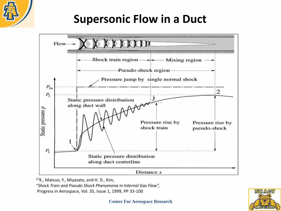
E: The Pseudo Shock Train Problem

A characteristic of supersonic internal flows is the development of a strong shock wave that forms as a result of

the flow interaction with the boundary layer along the wall surface of the device. The shock is bifurcated and a

series of repeated shocks is formed along the flow passage. The number of these shock series and their position in

the flow passage is dependent on the freestream Mach number, the pressure conditions imposed at both the upstream

and downstream locations of the flow passage, the passage geometry, and the wall friction due to viscosity. This

phenomena was described in Om et al25

as „multiple shocks‟, by McCormick18

, as a „shock system‟, and most

recently by Carroll and Dutton26

, and Matsuo27

as a „pseodo-shock train’. Through the interaction region, the flow

can be decelerated from a supersonic flow to a subsonic flow. Figure 23 presents an illustration of the shock train

phenomenon in an internal duct. The shock train is clearly visible and is usually followed by an adverse pressure

gradient region in a long enough duct. The interaction region including both shock train and the subsequent pressure

recovery region is referred to as a „pseudo shock‟27

.

Figure 23: Schematic of Shock Train and Pseudo Shock27

Also presented in Figure 23 is the behavior of the static pressure at the wall and at the center line of the constant

area duct. Examination of this figure revels that the static wall pressure rises at a faster rate in the shock train

region, i.e. between points 1, j, than in the mixing region, i.e. between points j, 2. A similar trend (pressure rise) is

observed in the static pressure distribution along the duct centerline. The oscillations observed in the static pressure

distribution along the duct centerline are due to the presence of the successive shock series or shock train. Beyond

point j no shock exists and the pressures at the wall surface and at the centerline are essentially the same.

The pressure rise between the points 1 and j is caused by the shock train. If the flow is fully subsonic and

uniform at the point j, then the static pressure downstream of this point should decrease due to the frictional effect.

However, it should be noted that the shock train is followed by the “mixing region”, where no shocks exist. The

pressure increase in this region is due in some extent to the mixing of a highly non-uniform profile created by the

shock train. The static pressure reaches its maximum at point 2.

The results of this research effort are compared to the analysis conducted in Ref 28 since the input data are taken

from the same source. Refer to Figure 24. The results of the IDS study as they relate to the density, velocity and

pressure distribution profiles are presented in Figures 25 and 26. Again, it can be seen that the IDS procedure

reproduces the expected flow field behavior.


13

Figure 24: Velocity vectors imposed on density contours, Ref. 28

Figure 25: IDS generated Velocity vectors imposed on density contours

Figure 26: IDS generated pressure contours for the Pseudo-Shock Train Problem

V. Conclusion

In an effort to improve the efficiencies of Computational Fluid Dynamic tools a new numerical computational

scheme/framework has been developed and is introduced. The „Intergo-Differential Scheme‟, IDS is a numerical

procedure based on two fundamental types of control volumes, spatial and temporal cells. This new scheme was

tested and validated on a chosen set of fluid dynamics problems and the results presented above. These problems

are listed as follows: the Hypersonic Leading Edge problem, the incompressibility Lid Driven Cavity problem, the

Shock Boundary Layer Interaction Problem, and the Isolator Pseudo-Shock Train problem. The solutions

obtained for these problems using the IDS procedure showed very good agreement with the physical expectations


14

and experimental data for each problem. A survey of CFD literature indicated that a large percentage of the

compressible flow field solvers encountered convergence difficulties when utilized to solve incompressible flow

problems29

. In an effort to demonstrate the capability of the IDS scheme the incompressible lid driven cavity

problem was addressed. The IDS scheme delivered excellent results for this problem without any convergence

difficulties. In addition, the IDS scheme was used to solve a pseudo-shock train problem which is considered

among one of the most challenging problems encountered in computational fluid dynamics29

. Once again, the

IDS procedure predicted excellent results. In conclusion, the solutions obtained for compressible external and

internal flows, and the incompressible lid driven cavity problem validates the IDS procedure as a robust, efficient,

and capable scheme that can solve a variety of complex fluid dynamics problems.

Acknowledgments

This work has been partially sponsored by the following agencies; AFRL/WPAB and NASA Glenn Research

Center. In addition, special appreciation is extended to Mr. Donnie Saunders of the Air Vehicles Directorate at

Wright Patterson Air Force Base and Dr. Isaiah M. Blankson of NASA Glenn Research Center for their

encouragement and support of this project.

References 1Frederick Ferguson, Gafar Elamin and Mookesh Dhanasar; A Method of Consistent Averages for the Computational

Solution to the Fluid Dynamic Equations, 5th Conference on Computational Fluid Dynamic, CFD 2010. 2Frederick Ferguson, Gafar Elamin “A numerical solution of the NS equations based on the mean value theorem with

applications to aerothermodynamics”, The 9th International Conference on Advanced Computational Methods and Experimental

Measurements in Heat and mass Transfer, Wessex Institute of Technology, New Forest, UK , July 2006. 3http://www.csm.ornl.gov/workshops/Petascale07/, Workshop on Software Development Tools for Petascale Computing, 1-2

August 2007, Washington, DC 4Jack J. Dongarra, and David W. Walker, THE QUEST FOR PETASCALE COMPUTING, HIGH- PERFORMANCE

COMPUTING, COMPUTING IN SCIENCE & ENGINEERING, MAY/JUNE 2001. 5Bush, Richard J, et al, „Application of CFD to Aircraft Design‟, AIAA paper 86-2651, 1986. 6www.spscicomp.org/ScicomP14/talks/Sugavanam.pdf 7John D. Anderson, Jr., “Computational Fluid Dynamics-The Basics with Applications”, McGraw-Hill, Inc., 1995. 8D. A., Anderson, J. C., Tannehill, and R. H., Pletcher, “Computational Fluid Dynamics and Heat Transfer”, McGraw-Hill

Book Co., 1984. 9David C., Wilcox, “Basic Fluid Mechanics”, First Edition, DCW Industries Inc, 1997. 10David Pnueli., and Chaim Gutfinger, “Fluid Mechanics”, Cambridge University Press, 1992. 11P. D., Lax, K., and B., Wendroff, “Systems of Conservation Laws”, Communications on Pure and Applied Mathematics,

Vol. 13, PP. 217-237.

12R. D., Richtmyer, “A Survey of Difference Methods for Nonsteady Fluid Dynamics”, NCAR Technical Note 63-2, Boulder,

Colorado. 13R. W., MacCormack, “Current Status of Numerical Solutions of the Navier-Stokes Equations”, AIAA paper no. 85-0032,

1985. 14D.B. Spalding, “A Novel Finite Difference Formulation for Differential Expression Involving both First and Second

Derivatives”, International Journal of Numerical Methods, Vol. 4, PP. 551–559. 15M. Hafez, and D.A., Caughey, “Frontiers of Computational Fluid Dynamics”, World Scientific, 2005. 16U. Ghia, K. N. Ghia, and C. T. Shin, “High –Resolutions for Incompressible Flow using the Navier-Stokes Equations and a

Multigrid Method”, Journal of Computational Physics, Vol. 48, 1982, PP 387-441. 17Stephen Akwaboa, “Navier-Stokes Solver for a Supersonic Flow over a Rearward-Facing Step”, M. S. Thesis, (Department

of Mechanical Engineering, North Carolina A & T State University, Greensboro, 2004). 18D. C., McCormick, “Shock/Boundary Layer Interaction Control with Vortex Generator and Passive Cavity”, AIAA

Journal, Vol. 31, Issue 1, 1993, PP 91-96. 19Maurice Rasmussen, and David Ross Boyd, “Hypersonic Flow”, John Wiley & Sons Inc., 1994. 20Y. H. Choi, C. L. Merkle, “The Application of Preconditioning in Viscous Flows”, Journal of Computational Physics, Vol.

105, 1993, PP 207-223. 21D. Vigneron, J. M. Vaassen, and J.A. Essers, “An Implicit Finite Volume Method for the Solution of 3D Low Mach Number

Viscous Flows using a Local Preconditioning Technique”, Journal of Computational and Applied mathematics, Vol. 215, 2008,

PP 610-617 22Zeng-Chang et al., The CE/SE Method for Navier-Stokes Equations Using Unstructured Meshes for Flows at All Speeds.,

AiAA 2000-0393.

http://www.csm.ornl.gov/workshops/Petascale07/


15

23R. S. Amano and D Sun, „Numerical Simulation of Supersonic Flowfield with Secondary Injection‟, 24th International

Congress of the Aeronautical Sciences, ICAS 2004. 24Valero Viti and Joseph Schetz, „Comparison of the First and Second Order Turbulence Models for a Jet/3D Ramp

Combination in Supersonic Flow‟, AIAA 2005-1100. 25D. Om, and M. E. Childs, “Multiple Transonic Shock Wave/Boundary Layer Interaction in a circular Duct”, AIAA Journal,

Vol. 23, Issue 5, 1985, PP 1506-1511. 26B. F., Carroll, and J. C., Dutton, “Characteristics of Multiple Shock Wave/ Turbulent Boundary Layer Interactions in

Rectangular Ducts”, Journal of Propulsion and Power, Vol. 6, Issue 2, 1990, PP 186-193. 27K., Matsuo, Y., Miyazato, and H. D., Kim, “Shock Train and Pseudo Shock Phenomena in Internal Gas Flow”, Progress in

Aerospace, Vol. 35, Issue 1, 1999, PP 33-100. 28Itaru Hataue, “Computational study of the shock wave boundary-layer interaction in a duct”, North Holland, Fluid

Dynamics Research 5 (1989) 217-234 29 Elamin, Gafar, „The Integral Differential Scheme (IDS): A New CFD Solver for the System of Navier-Stokes Equations

with Applications‟, Dissertation 2008

Center For Aerospace Research

Validation and Verification of the Navier-Stokes Solutions

Obtained from the Applications of the


AIAA 2011

Presenter: Mookesh Dhanasar, Ph.D. Contributors: Fredrick Ferguson, Ph.D., Nasstaja Dasque

Department of Mechanical Engineering North Carolina Agricultural and Technical State University

Jul-14 1

http://www.google.com/imgres?imgurl=http://4.bp.blogspot.com/_aXwvjOCyM24/Sc_g1L_OdGI/AAAAAAAAMHE/Pp421RbLZj4/s320/NCAT+logo+2.jpg&imgrefurl=http://meacswacsports.blogspot.com/2009_03_01_archive.html&usg=__teAzpn-UXh0eugdTN7BmVxMznXk=&h=179&w=259&sz=18&hl=en&start=28&um=1&itbs=1&tbnid=OYuTZnjgXKCPrM:&tbnh=77&tbnw=112&prev=/images?q=ncat+logo&start=20&um=1&hl=en&sa=N&ndsp=20&tbs=isch:1

http://www.google.com/imgres?imgurl=http://www.ncat.edu/events/spring10/aggie_nights/images/logo.jpg&imgrefurl=http://www.ncat.edu/events/spring10/aggie_nights/&usg=__tOyzDqVnP3llMNVOj_V947CH1W8=&h=246&w=306&sz=48&hl=en&start=46&um=1&itbs=1&tbnid=jZ-go7NGLwuwcM:&tbnh=94&tbnw=117&prev=/images?q=ncat+logo&start=40&um=1&hl=en&sa=N&ndsp=20&tbs=isch:1


Outline

1) Brief overview of CFD

2) Mathematical Overview of the


3) Test Cases

4) Conclusion



Center For Aerospace Research 3

Introduction • Historically only Analytical Fluid Dynamics (AFD) and

Experimental Fluid Dynamics (EFD).

• CFD is the computer simulation of fluid dynamic systems through

the use of engineering models (mathematical formulation) and

numerical methods (discretization methods and grid generations)

• CFD made possible by the advent of digital computer and advancing

with improvements of computer resources (1947, 500 Flops, 2003

Teraflops, 2003 2015 Petaflops?)

1947 - 500 flops Computer 2003 – 20 Teraflops Computer

Data, Ref. 2

Jul-14



http://rds.yahoo.com/_ylt=A9G_bDpNkRFMfTsAVd2JzbkF;_ylu=X3oDMTBqaTFoaGxvBHBvcwMxNwRzZWMDc3IEdnRpZAM-/SIG=1iumgbknh/EXP=1276306125/**http:/images.search.yahoo.com/images/view?back=http://images.search.yahoo.com/search/images?p=1946+eniac+computer&sado=1&ei=utf-8&fr=yfp-t-892-s&fr2=sg-gac&w=485&h=343&imgurl=www.funkygoods.com/schwarzschild/2006_01/computer_02.jpg&rurl=http://www.funkygoods.com/schwarzschild/2006_01/2006_01_26.html&size=116k&name=computer+02+jpg&p=1946+eniac+computer&oid=f7f4dfdd08b3307c&fr2=sg-gac&no=17&tt=200&sigr=11va100ep&sigi=11o4b1mhj&sigb=13cnplj42

http://www.google.com/imgres?imgurl=http://farm2.static.flickr.com/1065/1263416314_828437de03.jpg&imgrefurl=http://flickr.com/photos/deegoo/1263416314/&usg=__X00ckh8Dw1gpzmAUmziPgzAiKQA=&h=375&w=500&sz=211&hl=en&start=2&um=1&itbs=1&tbnid=62Fgix-Ms78myM:&tbnh=98&tbnw=130&prev=/images?q=CERN+super+computers&um=1&hl=en&sa=N&tbs=isch:1


Why use CFD?

1. Engineering: Analysis and Design A. 1. Simulation-based design instead of “build & test”

More cost effective and more rapid than EFD

CFD provides high-fidelity database for diagnosing flow field

B. 2. Simulation of physical fluid phenomena that are difficult for experiments

Full scale simulations (e.g., automobile, ships and airplanes)

Environmental effects (wind, weather, etc.)

Hazards (e.g., explosions, radiation, pollution)

Physics (e.g., planetary boundary layer, stellar evolution)

2. Exploration: Knowledge of flow physics

Data, Ref. 2

Jul-14




Where is CFD used?

• Aerospace

• Automotive

• Biomedical

• Chemical

Processing

• HVAC

• Hydraulics

• Marine

• Oil & Gas

• Power

Generation

• Sports

Data, Ref. 3

Jul-14




Example of the Importance of CFD to the Aero-Industry

Ref. 4 Data

Jul-14




CFD Challenges?

Ref. 4 Data

Long Cycle Times Due to

1. Grids Generation Req. &

2. Fidelity of Simulation Tools

Engineering Perspective: Analysis, Not Design

Jul-14




Distribution of Current Turbulence Usage

Ref. 5 Data

-Use DNS/LES Data to Develop Turbulence Models for Cartesian Grid Systems

Why Cartesian Grids? -fast grid generation, numerical & memory efficiency during parallelization

Why Algebraic Turbulence Models? -numerical & memory efficiency -capture the basic physics of the process

Research Goal: Develop Algebraic Turbulence Models

Jul-14

Computer Speed vs. Time (Year)



Center For Aerospace Research Jul-14 9

The Integral Form of the Equations

kwjviuV

kdxdyjdxdzidydzsd

kqjqiqq zyx

2

2VeE

v s

sdVdvt

0

sdsPdVsdVdvVt

sssv

ˆ.

ssssv

sdqsdVsdVPsdVEEdvt

...

where

zzzyzx

yzyyyx

xzxyxx

, ,




x

v

y

uyxxy

x

w

z

uzxxz

z

v

y

wzyyz

x

Tkqx

y

Tkq y

z

Tkqz

Viscous Relations

Equations and formulas from: J. D. Anderson(1995) : “Computational Fluid Dynamics-The basics with applications”, McGraw-Hill, Inc.

z

w

y

v

x

uxx 2

3

2

z

w

x

u

y

vyy 2

3

2

y

v

x

u

z

wzz 2

3

2




The Closed System of the Equations

The closed system of the equations has only five unknowns

Twvu ,,,,

Additional relations

Equation of state

Internal energy

Sutherland’s law for viscosity

Prandtl number

RTP

TCe v

K

Cp

Pr

110

1105.1

T

T

T

T




IDS Control Volume Representation

i,j,k

z

x

y

Jul-14 12

Points

Cells

Control Volume

Key Features




Mass Conservation in relations to Cell

i

Surface

iSurfaceCenterCell

dsnVt

dV

6

SurfacesCellatFluxesLocalFCenterCellatFluxesofGradient

usu min

plusv

plusu

usv min

v s

sdVdvt

0

usw min

plusw

plus

us

plus

us

plus

us

average

cell

wwww

wwww

z

vvvv

vuvv

y

uuuu

uuuu

xt

4321

min4321

4321

min4321

4321

min4321

4

1

4

1

4

1

Jul-14




IDS Implementation Steps

E

w

v

u

U

U

U

U

U

U m

5

4

3

2

1

tdt

dUUU

kji

mt

kjim

tt

kjim

,,

,,,, )()(

Construct the solution using Taylor Series Expansion

Treat each eight cells as a control volume of center i,j,k and evaluate the generic function U as an arithmetic average of its value at the centers of the eight cells.

8

1

,,8

1

cell

average

cell

t

kji UU

In another consistence averaging process, the time derivative at node i,j,k is obtained as an arithmetic average of the time derivatives at the cell centers.

8

1,,8

1

cell cell

m

kji

m

dt

dU

dt

dU

Jul-14




1

222,,

'

222,

,,,,,,

,,

111

Re

2

111

zyx

zyxa

z

w

y

v

x

u

t

kji

L

ji

kjikjikji

kjiCFL

Use the following CFL Criterion to evaluate the time step

kji

kjikji

kji

,,

,,,,

,,'

Pr/,3

4

max

tdt

dUUU

kji

mold

kjim

new

kjim

,,

,,,, )()( Update the solution

Decouple the new variables

new

kji

new

kji U,,1,,

new

kji

new

kjiU

Uu

,,1

2,,

new

kji

new

kjiU

Uv

,,1

3,,

new

kji

new

kjiU

Uw

,,1

,,

4

2

,,

222

1

5,, 1

2

M

wvu

U

UT

new

kji

new

kji

IDS Implementation Steps

Jul-14




Test Case 1: Supersonic Flow over a flat plate




Q2 Q1 Q3

5.4M

Inflow Cdts Outflow Cdts

Far field Cdts

Flat Plate

Mach 4.5 Flow Over A Flat Plate

Grid Independence Studies

Code Validation and Verification Studies

Leading & Trailing Edge Studies

Test Problem: Subsonic, Transonic & Supersonic/Hypersonic Flat Plate

72.0Pr,10*2.7Re,5.4 6 LM

Sym Sym

Objectives:

Jul-14




x-NonDim

Tem

per

atu

re-

Non

Dim

0 0.5 1 1.5 20.7

0.8

0.9

1

1.1

1.2

Grid101

Grid201

Grid301

Grid401

Grid501

Frame 001 03 Jun 2010

Mach 4.5 Grid Temperature Studies

x-NonDim

V-v

eloci

ty-

No

nD

im

0 0.25 0.5 0.75 1 1.25 1.5 1.75 2

-0.14

-0.12

-0.1

-0.08

-0.06

-0.04

-0.02

0

Grid101

Grid201

Grid301

Grid401

Grid501

Frame 001 03 Jun 2010

Mach 4.5 Grid v-Velocity Studies

Mach 4.5 Grid Density Studies

x-NonDim

Den

sity

-N

onD

im

0 0.5 1 1.5 2

0.5

0.6

0.7

0.8

0.9

1

1.1

1.2

1.3

1.4

1.5

1.6

1.7

Grid101

Grid201

Grid301

Grid401

Grid501

Frame 001 03 Jun 2010

x-NonDim

U-v

eloci

ty-

No

nD

im

0 0.25 0.5 0.75 1 1.25 1.5 1.75 20

0.1

0.2

0.3

0.4

0.5

0.6

0.7

0.8

0.9

1

Grid101

Grid201

Grid301

Grid401

Grid501

Frame 001 03 Jun 2010

Mach 4.5 Grid u-Velocity Studies

Grid Independence Studies

72.0Pr,10*2.7Re,5.4 6 LM

Jul-14




Mach 4.5 Flow Field Parameters Over Flat Plate

Density: 1.04545 1.14193 1.23842 1.3349 1.43138 1.52787 1.62435 1.72084

Frame 001 03 Jun 2010

V-Velocity: 0.00950367 0.0290327 0.0485618 0.0680908

Frame 001 03 Jun 2010

Density Contour V-Velocity Contour

Temperature: 1.00952 1.04639 1.08325 1.12011 1.15697 1.19383 1.23069 1.26755

Frame 001 03 Jun 2010

U-Velocity: 0.143421 0.286841 0.430262 0.573683 0.717104 0.860524

Frame 001 03 Jun 2010

U-Velocity Contour Temperature Contour

72.0Pr,10*2.7Re,5.4 6 LM

Jul-14




Pressure: 1.0768 1.31566 1.55452 1.79339 2.03225

Frame 001 04 Jun 2010

Mach 4.5 Pressure Field Over Flat Plate

72.0Pr,10*2.7Re,5.4 6 LM

Jul-14




Mach 4.5 Density Profiles on Flat Plate

Density - NonDim

y-

No

nD

im

0.9 1 1.1 1.2 1.3 1.40

0.1

0.2

0.3

0.4

0.5

Q1-Density

Q2-Density

Q3-Density

Frame 001 03 Jun 2010

Q2 Q1 Q3

5.4M

72.0Pr,10*2.7Re,5.4 6 LM

Adiabatic Conditions

Jul-14




U-Velocity - NonDim

y-

Non

Dim

0 0.1 0.2 0.3 0.4 0.5 0.6 0.7 0.8 0.9 10

0.1

0.2

0.3

0.4

0.5

Q1-uVelocity

Q2-uVelocity

Q3-uVelocity

Frame 001 03 Jun 2010

Q2 Q1 Q3

5.4M

Mach 4.5 u-Velocity Profiles on Flat Plate

72.0Pr,10*2.7Re,5.4 6 LM


Jul-14




V-Velocity - NonDim

y-

Non

Dim

-0.01 0 0.01 0.02 0.03 0.04 0.05 0.06 0.070

0.1

0.2

0.3

0.4

0.5

Q1-vVelocity

Q2-vVelocity

Q3-vVelocity

Frame 001 03 Jun 2010

Q2 Q1 Q3

5.4M

Mach 4.5 v-Velocity Profiles on Flat Plate

72.0Pr,10*2.7Re,5.4 6 LM


Jul-14




Temperature - NonDim

y-

Non

Dim

0.98 1 1.02 1.04 1.06 1.08 1.1 1.12 1.140

0.1

0.2

0.3

0.4

0.5

Q1-Temperature

Q2-Temperature

Q3-Temperature

Frame 001 03 Jun 2010

Q2 Q1 Q3

5.4M

Mach 4.5 Temperature Profiles on Flat Plate

72.0Pr,10*2.7Re,5.4 6 LM


Jul-14




Flat Plate - Leading Edge Effects

Normal Shock Wave Due to Leading Edge/Boundary Layer Development

Flow Field Expansion Due to High Pressure Boundary Layer Compression

x-NonDim

y-N

onD

im

0.4 0.5 0.6 0.7 0.80

0.01

0.02

0.03

0.04

0.05 Pressure

2.1811

2.0010

1.8209

1.6408

1.4607

1.2806

1.1006

0.9205

0.7404

0.5603

0.3802

Frame 001 05 Jun 2010

x-NonDim

y-N

on

DIm

0.4 0.5 0.6 0.7 0.80

0.01

0.02

0.03

0.04

0.05

Density

1.6845

1.6000

1.5154

1.4308

1.3463

1.2617

1.1772

1.0926

1.0080

0.9235

0.8389

0.7544

0.6698

0.5853

0.5007

Frame 001 05 Jun 2010

Pressure Density 72.0Pr,10*2.7Re,5.4 6 LM


Observations:

Jul-14




Flat Plate - Leading Edge Effects

x-NonDIm

y-N

onD

im

0.5 0.6 0.70

0.01

0.02

0.03

0.04

0.05

U-velocity

0.946157

0.88308

0.820003

0.756925

0.693848

0.630771

0.567694

0.504617

0.44154

0.378463

0.315386

0.252308

0.189231

0.126154

0.0630771

Frame 001 05 Jun 2010

x-NonDIm

y-N

onD

im

0.5 0.6 0.70

0.01

0.02

0.03

0.04

0.05V-Velocity

0.0754

0.0483

0.0187

0.0078

0.0015

-0.0257

-0.0553

-0.0849

-0.1145

-0.1440

Frame 001 05 Jun 2010

u-Velocity V-Velocity 72.0Pr,10*2.7Re,5.4 6 LM

Normal Shock Wave Due to Leading Edge/Boundary Layer Development

Flow Field Expansion Due to High Pressure Boundary Layer Compression

Observations:


Jul-14




x-NonDIm

y-N

onD

im

1.4 1.45 1.5 1.55 1.6 1.65 1.70

0.025

0.05

0.075

0.1

0.125

0.15

0.175

0.2

0.225

0.25V-Velocity

0.0630616

0.0482682

0.0334749

0.0186815

0.00388812

-0.0109053

-0.0256986

-0.040492

-0.0552854

-0.0700788

-0.0848721

-0.0996655

-0.114459

-0.129252

-0.144046

Frame 001 05 Jun 2010

x-NonDIm

y-N

onD

im

1.4 1.45 1.5 1.55 1.6 1.65 1.70

0.025

0.05

0.075

0.1

0.125

0.15

0.175

0.2

0.225

0.25U-velocity

0.946157

0.88308

0.820003

0.756925

0.693848

0.630771

0.567694

0.504617

0.44154

0.378463

0.315386

0.252308

0.189231

0.126154

0.0630771

Frame 001 05 Jun 2010

Flat Plate - Trailing Edge Effects

Hypersonic Trailing Edge/Boundary Layer Interaction: Flow Field Expansion

72.0Pr,10*2.7Re,5.4 6 LM


Jul-14




x-NonDim

y-N

onD

im

1.4 1.5 1.6 1.7 1.80

0.01

0.02

0.03

0.04

0.05

U-velocity: 0.033 0.130 0.228 0.326 0.423 0.521 0.619 0.716 0.814 0.912

Frame 001 05 Jun 2010

72.0Pr,10*2.7Re,5.4 6 LM

Flat Plate - Trailing Edge Effects

x-NonDim

y-N

onD

im

1.4 1.5 1.6 1.7 1.80

0.01

0.02

0.03

0.04

0.05

V-Velocity: -0.151 -0.128 -0.105 -0.082 -0.060 -0.037 -0.014 0.009 0.032 0.055

Frame 001 05 Jun 2010

72.0Pr,10*2.7Re,5.4 6 LM

Hypersonic Trailing Edge/Boundary Layer Interaction: Flow Field Expansion


Jul-14




Influence of Temperature Boundary Conditions on Flowfield

x-NonDim

Den

sity

0 0.5 11

1.1

1.2

1.3

1.4

1.5

1.6

1.7

1.8

1.9

2

2.1

2.2

2.3

Adiabatic Wall

Constant Wall

Frame 001 07 Jun 2010

x-NonDIm

Pre

ssure

0 0.5 11

1.2

1.4

1.6

1.8

2

2.2

2.4

2.6

Adiabatic Wall

Constant Wall

Frame 001 07 Jun 2010

x-NonDIm

Tem

per

ature

0 0.5 1

1

1.1

1.2

Adiabatic Wall

Constant Wall

Frame 001 07 Jun 2010

Adiabatic & Constant Wall Conditions

Jul-14




Test Case 2: Incident Shock Wave Boundary Layer Interaction




Ref: Experimental Study of an Incident Shock Wave/Turbulent Boundary Layer Interaction Using PIV, R.A. Humble,* F. Scarano,† and B.W van Oudheusden‡ Delft University of Technology, 2629 HS Delft, The Netherlands

Incident Shock Wave Boundary Layer Interaction

IDS-NCAT Results




Non-Dim u-Velocity Contour/Velocity Vector Plots

Non-Dim u-vel plots




Non-Dim v-Velocity Contour/Velocity Vector Plots

Non-Dim v-vel plots




Test Case 3: Supersonic Jet Interaction




Ref. 24: Viti et al, “Detailed Flow Physics of the Supersonic Jet Interaction Flow Field”

Supersonic Jet Interaction




Supersonic Jet Interaction Ref. 24: Viti et al, “Detailed Flow Physics of the Supersonic Jet Interaction Flow Field”




Test Case 4: Supersonic Flow in a Duct




27K., Matsuo, Y., Miyazato, and H. D., Kim, “Shock Train and Pseudo Shock Phenomena in Internal Gas Flow”, Progress in Aerospace, Vol. 35, Issue 1, 1999, PP 33-100

Supersonic Flow in a Duct




Ref. SHOCK TRAIN, Fluid Dynamics Research 5 (1989) 217-234, North-Holland “Computational Study

of the Shock Wave Boundary-layer Interaction in a duct”

Shock Wave Boundary-Layer Interaction in a Duct

Velocity vectors imposed on density contours (a) paper (b) IDS results




Ref. SHOCK TRAIN, Fluid Dynamics Research 5 (1989) 217-234, North-Holland “Computational Study

of the Shock Wave Boundary-layer Interaction in a duct”

Shock Wave Boundary-Layer Interaction in a Duct




Conclusions

A new numerical scheme for solving the complete three dimensional form of the system of the Navier-Stokes equations was developed.

The ability of the scheme to solve different flow types was tested on compressible external flow, Incompressible flow, and internal compressible flow applications.

In all cases the results showed very good agreement with the physical expectation of the flow, and the experimental data.

This agreement solidified the belief that the scheme is robust, efficient, and capable of solving a variety of complex fluid dynamics problems.

The FORTRAN program can be modified to run on multiple platforms Extension of IDS to Arbitrary Geometries and to include other phenomena

such as turbulence and finite rate chemistry is recommended.

Even though the scheme generates impressive results using the available version of CFL criterion a complete stability analysis is recommended to determine the appropriate CFL criterion for the scheme.

Jul-14




Length

Width

Height

The x Component Velocity Distribution on Nine Planes Cavity Velocity Vectors on Three XY Planes

The Lid Driven Cavity Problem




IDS Solution Vigneron et. Al. Solution

The Lid Driven Cavity Problem: Streamlines Plot

Flow




The Lid Driven Cavity Problem : Validation

0.0

0.1

0.2

0.3

0.4

0.5

0.6

0.7

0.8

0.9

1.0

-0.3 0.0 0.3 0.5 0.8 1.0

IDS results Choi & Merkle (1995) Vigneron et al. (2008)

-0.20

-0.15

-0.10

-0.05

0.00

0.05

0.10

0.15

0.20

0.00 0.20 0.40 0.60 0.80 1.00

IDS Results Choi & Merkle (1995) Vigneron et al.

The x Component Velocity Profile along the Vertical Centerline of the Cavity

The y Component Velocity Profile along the Horizontal Centerline of the Cavity



Validation and Verification of the Navier-Stokes Solutions Obtained from the Applications of the...

Documents

Transcript of Validation and Verification of the Navier-Stokes Solutions Obtained from the Applications of the...