Truncated Navier-Stokes Equations with the Automatic Filtering

March 17, 2010 5:4 Journal of Turbulence paper˙TD09˙jot˙031110

Journal of TurbulenceVol. 00, No. 00, 200x, 1–23

RESEARCH ARTICLE

Large Eddy Simulations Using Truncated Navier-Stokes

Equations with the Automatic Filtering Criterion

T. Tantikula,∗ and J.A. Domaradzkia,∗∗

aDepartment of Aerospace and Mechanical Engineering, University of SouthernCalifornia, Los Angeles, CA. 90089-1191

(Received 00 Month 200x; final version received 00 Month 200x)

We propose a Large Eddy Simulation (LES) technique based on previously developedTrancated Navier Stokes (TNS) method. In TNS the Navier Stokes equations are solvedthrough a sequence of direct numerical simulation runs and a periodic processing of smallscales to provide the necessary dissipation. In the simplest case the processing is accomplishedby filtering the turbulent fields with a properly chosen filter. In the previous work the periodfor processing was selected in advance for each case using heuristic arguments validated bytrial and error. In this work we develop a criterion that automates the selection of a timeinstant in simulations when the processing occurs. The criterion is based on the relationshipbetween the energy of the flow field and the energy of the same field filtered with the chosenfilter. The procedure is tested in LES of the turbulent channel flow performed at variousReynolds numbers and in domains of different sizes for which DNS and experimental data areavailable for comparison.

Keywords: Large Eddy Simulations; Truncated Navier-Stokes Equations; ExplicitFiltering; Automatic Filtering Criterion

1. Introduction

Several classifications of subgrid-scale (SGS) models for LES have been proposedin the literature on the subject. In a review paper of Domaradzki and Adams [1]the SGS models are divided into two general categories: the traditional models thatuse the explicit expressions for the SGS terms, the SGS stress tensor in particular,and the models that construct the unknown primitive variables such as velocity inorder to use these variables to compute the SGS terms directly from the definitions.The traditional SGS modeling approaches can be subdivided into three groups: theeddy viscosity models, the similarity models, and the mixed models. The examplesof the models in the other group are the velocity estimation model proposed byDomaradzki et al. [2, 3] and the approximate deconvolution model (ADM) of Stolzet al. [4]. Kosovic et al. [5] divided SGS models into three groups, characterized bythe use of explicit filtering. First are the models that use an explicit SGS expressionbut do not employ explicit filtering, for instance the classical Smagorinsky eddyviscosity model. Second are the models that use an explicit SGS expression andemploy explicit filtering, e.g., the dynamic Smagorinsky model. The third categoryare the so-called implicit models because equations of motion are solved without

∗ Email : [email protected]∗∗ Email : [email protected]

ISSN: 1468-5248 (online only)c© 200x Taylor & FrancisDOI: 10.1080/14685240YYxxxxxxxhttp://www.informaworld.com


2

neither explicit filtering nor explicit SGS terms. Such approaches rely on the prop-erties of the numerical scheme to provide implicit dissipation and are known asMonotone Integrated Large Eddy Simulations (MILES) or Implicit Large EddySimulations (ILES). In depth review of ILES is given in the monograph edited byGrinstein et al. [6]. For high order, nondissipative numerical schemes this classifi-cation can be extended to include models that do not use explicit SGS terms butemploy the explicit filtering to model the effects of SGS dissipation. The modelingapproach discussed in this paper belongs to this group and originated from the SGSvelocity estimation model proposed by Domaradzki and Saiki [2]. The model wasdeveloped in spectral space representation and later implemented in the physicalspace by Domaradzki and Loh [7].

The original velocity estimation model encountered difficulties in LES of highReynolds number flows because it did not produce enough SGS dissipation. Toaddress this shortcoming Domaradzki et al. [3] introduced the modification of thevelocity estimation model which solves LES equations in parallel with the Trun-cated Navier Stokes (TNS) equations on a finer mesh; TNS provides the estimatedvelocity that is used to compute the SGS stress tensor needed in LES. More specif-ically, the TNS equations are just Navier-Stokes equations discretized on a meshby a factor of two smaller than LES equations of interest. The estimated veloc-ity to be advanced in TNS is obtained in two steps. First, the velocity from LESis ’de-filtered’, providing large scale velocity represented on a coarse LES mesh.Second, the small scale perturbation velocity is created by nonlinear interaction ofthe reconstructed field. The total estimated velocity is a sum of both parts and isrepresented on a finer TNS mesh. The estimated velocity is advanced in time usingTNS equations, i.e., using a Navier-Stokes solver on the fine mesh. The velocityfield from TNS is then used at each time step to compute the SGS stress termdirectly from the TNS field, and this SGS stress is used to advance in time LESequations. This process of two parallel runs is continued for some fixed time periodT until the accumulation of energy in the small scales of TNS begins to affect thelarge scales. To assure the accurate large scale results the whole process has to bereinitialized every time period T, with reduced energy in the small scale regionobtained by a low pass filter. The results from LES for homogeneous turbulenceand turbulent channel flow test cases are in a very good agreement with the DNSand experimental data. The disadvantage of this approach is that the procedure isquite complicated and requires more computational time compared to other LESmodeling approaches because additional TNS equations must be solved. However,a significant speed up of computations is possible for a simplified version of themodel that employs only TNS equations as shown by Domaradzki et al. [3]. Sucha simplification is based on the observation that TNS velocity on the fine meshalready contains information about large scales of the flow and thus LES equationsare redundant. Since the small scales of TNS fields are subjected to periodic fil-tering the physical meaning is ascribed only to the large TNS scales, given on thecoarse LES mesh. In this approach the estimated small scale velocity field providesthe SGS effects on the large scales via nonlinear interactions in the Navier-Stokesequations. The approach is less complicated in term of the numerical implementa-tion and retains the same quality of the results as the original method. However,the user still needs to specify the time period T for filtering and re-initializationof TNS in order to prevent the accumulation of energy in the small scales andthe resulting error propagating toward the large scales and contaminating them.Our goal in this work is to investigate a procedure that determines the period Tautomatically, without a need to provide its value as a parameter by the user. Oncethe procedure is defined in the next section it will be subsequently tested in LES


3

of the turbulent channel flow problem in the following sections.The explicit filtering as a LES tool has been employed in different forms previ-

ously, usually as a method to control numerical instabilities. Visbal and Rizzetta[8], [9] studied the application of a high order finite difference method to LES ofcompressible flows. They used 4th and 6th order compact differencing schemes forspatial discretization and different explicit and implicit time marching methods.The simulations were performed with the unfiltered Navier-Stokes equations andthe high order Pade type low pass spatial filter was employed at each timestepto remove spurious high frequency modes which arise because of the lack of thedissipation in the spatial discretization. It was found that the compact/filteringscheme performed better or comparably to the constant coefficient and dynamicSmagorinsky models for a number of different turbulent flows. Bogey and Bailly [10]investigated jet flows using LES with explicit filtering. The numerical simulationswere performed using a low dissipation numerical scheme with the explicit fourthorder 13-point centered finite differences for spatial discretizations and the secondorder six stage low storage Runge-Kutta algorithm for time integration. The ex-plicit selective/high-order filtering was employed to emulate the dissipative effectsof the neglected subgrid scales. Interestingly, the filtering was not applied at everytime step but every second or third time step. The results from the simulationswith the filtering applied at every two or three iterations exhibit no relationshipbetween the frequency of application of the filtering and the quality of the results.When spectral methods, which have negligible numerical dissipation, are employedto simulate high Reynolds number flows often explicit filters and penalty techniquesmust be used to stabilize numerics, e.g., in Diamessis et al. [11], and in Minguezand Pasquetti [12]. Such methods are known as stabilized LES and use filteringat each time step. The numerical dissipation associated with one of these methodshas been investigated recently by Diamessis et al. [13]. In using such techniquesone must recognize that achieving numerical stability does not necessarily implyphysically correct results. Therefore, such techniques must always be validated bycomparing results they produce with experiments and DNS results.

In the work described here we use spectral methods stabilized by weak, explicitfilter applied at each time step and much less frequent periodic filtering that is usednot as a stabilization tool but primarily as a SGS modeling tool based on physicalconsiderations of the energy transfer and spectra in developed turbulence.

2. Filtering and filtering criterion

In LES the filtering operation is applied to a full, turbulent velocity field, to sepa-rate it into large, resolved scales and small, subgrid scales. Ideally, the filter shouldretain complete information about large scales and substantially remove or atten-uate small scales, allowing the user to focus the computational power on the largescales. Because the computational space in the simulations is discrete, filters aregiven in the discrete form as well. A convenient filter with desirable properties hasbeen proposed by Stolz et al.[4] for the Approximate Deconvolution Model (ADM).If G represents the primary filter used, the filtering operation can be written in thephysical space as

u(x) = G ∗ u =∫ ∞−∞

G(x− x′)u(x′)dx′ (1)

and in the spectral space as


4

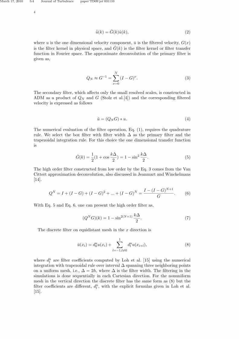
ˆu(k) = G(k)u(k), (2)

where u is the one dimensional velocity component, u is the filtered velocity, G(x)is the filter kernel in physical space, and G(k) is the filter kernel or filter transferfunction in Fourier space. The approximate deconvolution of the primary filter isgiven as,

QN ≈ G−1 =N∑ν=0

(I −G)ν . (3)

The secondary filter, which affects only the small resolved scales, is constructed inADM as a product of QN and G (Stolz et al.[4]) and the corresponding filteredvelocity is expressed as follows

u = (QNG) ∗ u. (4)

The numerical evaluation of the filter operation, Eq. (1), requires the quadraturerule. We select the box filter with filter width ∆ as the primary filter and thetrapezoidal integration rule. For this choice the one dimensional transfer functionis

G(k) =12

(1 + cosk∆2

) = 1− sin2 k∆2. (5)

The high order filter constructed from low order by the Eq. 3 comes from the VanCittert approximation deconvolution, also discussed in Jeanmart and Winckelmans[14].

QN = I + (I −G) + (I −G)2 + ...+ (I −G)N =I − (I −G)N+1

G. (6)

With Eq. 5 and Eq. 6, one can present the high order filter as,

(QNG)(k) = 1− sin2(N+1) k∆2. (7)

The discrete filter on equidistant mesh in the x direction is

u(xi) = du0u(xi) +1∑

l=−1,l 6=0

dul u(xi+l), (8)

where dul are filter coefficients computed by Loh et al. [15] using the numericalintegration with trapezoidal rule over interval ∆ spanning three neighboring pointson a uniform mesh, i.e., ∆ = 2h, where ∆ is the filter width. The filtering in thesimulations is done sequentially in each Cartesian direction. For the nonuniformmesh in the vertical direction the discrete filter has the same form as (8) but thefilter coefficients are different, dnl , with the explicit formulas given in Loh et al.[15].


5

In a simulation with general finite difference schemes, the inability to representthe high wave number modes accurately results in the undesired dispersion er-ror. This error causes unphysical and rapid oscillations in the marginally resolvedregions which may lead to numerical instabilities and a break down of the simula-tion. To eliminate such spurious modes an artificial dissipation through additionaldamping terms is usually employed. The spectral methods used in this work are wellknown for high accuracy or spectral convergence. However spectral convergence isachieved only when the spectral methods are applied to sufficiently smooth prob-lems. The loss of fast convergence for the problems that have potential to developnonsmooth solutions in finite time undermines the advantages of spectral methods.Gottlieb and Hesthaven [16] reported the use of spectral filters acting in a similarfashion as additional dissipative terms that help to stabilize simulations withoutaffecting the spectral convergence. Besides the ability to retain the the spectralconvergence and stabilize the simulation, the filtering also decreases the aliasingerrors. According to Gottlieb and Hesthaven [16], there is no unique choice of thefilter function as long as certain basic requirements are satisfied. The baseline DNScode employed for simulations in this work has been developed by Diamessis et al.[11] and employs the exponential filter

σ(k) ={

1, 0 ≤ k ≤ klexp[−α( k−kl

N−kl)p], kl ≤ k ≤ N,

(9)

where p is the filter order, N is the highest mode in the spectral domain, kl is thefilter lag, and α = − log εM with εM being the machine precision. The filter (9)is intentionally selected such that it affects only the high frequency modes and itspurpose is only to stabilize the numerical simulation and enhance the convergencerate of the approximation.

The filtered solution fF may now be expressed in terms of the modes in Legendrespace of the numerical solution as:

fF =Nk−1∑j=0

σ(kj)fjPj(zj), (10)

where kj is the jth discrete Legendre mode. The filtering in Fourier space is donein the similar fashion [16].

Transfer functions for different filters described above are shown in figure 2. Bydesign, the exponential filter affects only modes in the vicinity of the mesh cutoff.The secondary filter (4) with N=5 retains almost all information for scales k ≤ kc,where kc = π/(∆) is the nominal cutoff wavenumber for the physical LES scales.This is the important characteristic of the secondary filter compared with othercandidate filters and it is chosen on this basis for the current work. The scalesbetween kc and the mesh cutoff 2kc = π/h are strongly attenuated by the filterand play a role of estimated subgrid scales in TNS.

The truncated Navier-Stokes equations (TNS) are equivalent to under resolvedDNS stabilized by the exponential filter (9). In under resolved DNS the energy willbegin to accumulate in small scales and the long time dynamics will be incorrect.The velocity estimation model (Domaradzki et al [3]) removes this accumulatedenergy by periodic filtering with the secondary filter of the form (4). The timeinterval between applications of the filter has to be manually prescribed by theuser in advance. The method would gain in generality if the filtering operation


6

Figure 1. One dimensional transfer function. Dash-dot line: explicit primary filter; dashed line: secondaryfilter with N=3; solid line: secondary filter with N=5; dotted line: spectral filter (9); vertical dashed line:filter cutoff wave number kc = π

∆.

could be activated automatically based on a physically established criterion.To establish such a criterion consider an energy spectrum E(k) for the full tur-

bulent velocity field and two secondary filters. The secondary filters are built fromthe primary filters with different filter widths. We choose two filter widths, h and∆, where h is the mesh size used in the simulation. The filter width h is related tothe grid cutoff wave number, khc , by the relation khc = π/h and the filter width ∆is related to the LES cutoff wave number, k∆

c , by the relation k∆c = π/(2h). The

filtered quantities obtained using the filters corresponding to cutoff wave numberskhc and k2h

c are denoted by tilde and hat, respectively. If the velocity field is filteredwith the former filter, the corresponding spectrum of the filtered field is denoted asE(k) and the energy removed by the filtering in a range of wavenumbers resolvedin TNS, up to khc = π/h is

I(h) =∫ kh

c

0(E(k)− E(k))dk, (11)

and the similar integral for the other filter. The expression

I(h)I(∆)

=

∫ khc

0 (E(k)− E(k))dk∫ khc

0 (E(k)− E(k))dk, (12)

is the ratio of energies removed by both filters in the range of wavenumbers resolvedin TNS. This ratio has been computed for progressively shallower energy spectra,


7

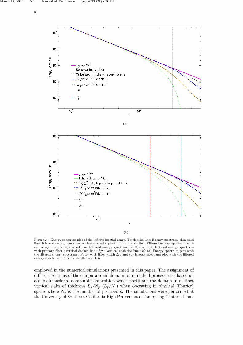
starting with the dissipation range spectrum form (Kerr [17]), the inertial rangek−5/3 spectrum, and the Batchelor’s k−1 spectrum. For illustration, in figure 2 (a)and (b) we plot the inertial range spectrum and the filtered energy spectra for twodifferent filter widths ∆. The results for the computed energy ratio are shown inTable 2. Depending on the spectrum, this ratio varies in the narrow range between0.007 and 0.010. We will use these bounds as guidelines to decide when the filteringin the simulations should be activated.

Table 1. Filtered energy ratios.

Energy spectrum Secondary filter ; N=5I(h)I(∆)

I(∆) I(h)Dissipation 0.0896 0.0061767 0.00689363Inertial 0.0234 0.00021466 0.009173504Batchelor 0.0699 0.00068 0.009728183

In actual TNS for turbulent channel flow, the energy ratio is computed from thesimulation data using the formula

〈 I(h)I(∆)

〉SIM (z) = 〈12

∑3n=1[(un − ¯un)(un − ¯un)]

12

∑3n=1[(un − ˆun)(un − ˆun)]

〉SIM , (13)

where 〈〉 is a plane averaged quantity, followed by integrating it over z:

I(h)I(∆)SIM

=∫ Lz

0〈 I(h)I(∆)

〉(z)dz. (14)

When this last quantity exceeds the theoretical value it is an indication that thesmall scales in TNS become too energetic. Therefore, when

I(h)I(∆)SIM

>I(h)I(∆)Theory

, (15)

the filtering will be activated to attenuate the small scales. This condition thusserves as the automatic filtering criterion in TNS.

3. Numerical simulations

The method is validated in this study by performing LES of the incompressibleturbulent channel flow because of the wealth of experimental and DNS data thatcan be used for comparison. The fluid is contained between two solid walls separatedby the distance Lz. The horizontal domain has the dimension Lx for the streamwisedirection and Ly for the spanwise direction. The no slip boundary conditions areimposed on the upper and lower walls and periodic boundary conditions in thehorizontal directions. The code uses a pseudospectral numerical method based onFourier expansions in the streamwise and spanwise directions and the Legendrepolynomials in the vertical direction, see Diamessis et al. [11]. In the numericalmethod used in this paper, the spectral filtering is applied in both Fourier andLegendre spaces to maintain the stability and spectral accuracy of the solutions,and also to help eliminate the aliasing effects. The MPI-based parallel solver was


8

(a)

(b)

Figure 2. Energy spectrum plot of the infinite inertial range. Thick solid line: Energy spectrum; thin solidline: Filtered energy spectrum with spherical tophat filter ; dotted line, Filtered energy spectrum withsecondary filter, N=5; dashed line: Filtered energy spectrum, N=3; dash-dot: Filtered energy spectrumwith primary filter ; vertical dashed line : k∆

c ; vertical dash-dot line : khc (a) Energy spectrum plot withthe filtered energy spectrum ; Filter with filter width ∆ , and (b) Energy spectrum plot with the filteredenergy spectrum ; Filter with filter width h

employed in the numerical simulations presented in this paper. The assignment ofdifferent sections of the computational domain to individual processors is based ona one-dimensional domain decomposition which partitions the domain in distinctvertical slabs of thickness Lx/Np (Ly/Np) when operating in physical (Fourier)space, where Np is the number of processors. The simulations were performed atthe University of Southern California High Performance Computing Center’s Linux


9

cluster. In order to reduce the total computational time and cost caused by theinterprocessor communication, the condition for automatic filtering indicated in(15) was checked at every 20 time steps while the spectral filtering was applied atevery time step in the simulations.

The TNS equations are standard Navier-Stokes equations for incompressibleflows

∂ui∂t

+∂uiuj∂xi

= −1ρ

∂p

∂xi+ ν

∂2ui∂xj∂xj

, (16)

∂ui∂xi

= 0, (17)

where the tilde notation is used to indicate that the spectral support for a givenquantity in discretized equations is not sufficient to capture all dynamically relevantscales of motion but is sufficient to resolve fields filtered with the filter (4). Thepressure term is decomposed into mean P (x) and fluctuating component p(x, t). Fora given, constant mean pressure gradient driving the flow the statistically steadystate is eventually established in which τ0 = −h(dP/dx), where τ0 is the wall shearstress. Introducing the shear velocity uτ = (τ0/ρ)1/2 the Navier-Stokes equationsare rewritten as follows

∂ui∂t

+∂uiuj∂xi

= −(1ρ

∂p

∂xi− u2

τ

hδ1i) + ν

∂2ui∂xj∂xj

. (18)

A statistically steady state is established much faster if the constant mass flux isimposed instead of the constant pressure gradient. The constant mass flux in thesimulations is enforced by setting the mean pressure gradient to the instantaneouswall shear stress at each time step, which is equivalent to using in Eq. (18) thefollowing expression for uτ

uτ (t) =

√−ν ∂〈u1〉

∂x3(Lz, t) + ν

∂〈u1〉∂x3

(0, t), (19)

where 〈...〉 indicates the plane averaged quantity. The above equations are normallynondimensionalized by the channel half width h = Lz

2 and the nominal friction ve-locity u0 = (τ0/ρ)1/2 for the constant pressure gradient case, i.e., τ0 = −h(dP/dx),giving

∂ui∂t

+∂uiuj∂xi

= −(1ρ

∂p

∂xi− u2

τδij) +1Re0

∂2ui∂xj∂xj

, (20)

∂ui∂xi

= 0, (21)

where Re0 = u0hν is the nominal Reynolds number. Note that the nominal Reynolds


10

Table 2. LES parameters

Case Domain size Resolution ∆x+ ×∆y+ ×∆z+1

cRe0 Reτ

I(∆)I(2∆)

Na NTb (NTNS/NDNS)d

Re180 4π × 2π × 2 64× 64× 65 35.34× 17.67× 0.84 180 182 0.008 24000 360− 580 0.069Re1050 2.5π × 0.5π × 2 96× 128× 65 85.93× 12.88× 4.90 1050 923 0.007 16000 350− 620 0.0056Re1050h 2.5π × 0.5π × 2 128× 128× 97 64.4× 12.88× 0.827 1050 967 0.007 22000 110− 180 0.0112Re1050h2 2.5π × 0.5π × 2 256× 128× 97 32.21× 12.88× 0.827 1050 967 0.007 19000 80− 160 0.0224Re2000S 2.5π × 0.5π × 2 96× 96× 211 163.62× 32.72× 0.33 2000 1690 0.008 15000 620− 980 0.0021Re2000L 7.5π × 3π × 2 256× 768× 131 184× 24.5× 0.86 2000 1699 0.009 28000 500− 1000 0.00153

a The total number of time steps until convergence to statistically steady state.b The observed frequency of the filtering operation (every NT time steps).c ∆z+

1 is the distance between the first grid point and the boundary.d N = Nx ×Ny ×Nz in TNS and baseline DNS rescaled to the same domain size.

Table 3. Parameters for the reference simulations.Case Domain size Resolution ∆x+ ×∆y+ ×∆z+ ReτTNSZ1 4π × 2π × 2 64× 64× 65 35.73× 17.88× 0.85 182TNSZ2 2.5π × 0.5π × 2 96× 128× 65 78.62× 11.79× 4.49 961HiDNS 3.6π × 1.9π × 2 160× 160× 129 14.85× 7.83× 0.063 210HiDNS2 8π × 3π × 2 6144× 4608× 633 8.3× 4.1× 8.9a 2003HiDNS3 8π × 3π × 2 3072× 2304× 385 7.6× 7.6× 0.032 944

a For HiDNS2 ∆z+ = ∆z+max; ; for all other cases ∆z+ is the distance between the

first grid point and the boundary.

number Re0 is used only as the parameter in the simulations and its value, whileclose, is usually different from the Reynolds number Reτ = uτh/ν based on the ac-tual friction velocity (19). Only in the statistically steady state in constant pressuregradient simulations Re0 = Reτ . The actual friction velocity nondimensionalizedby u0 is

uτ (t) =

√− 1Re0

∂〈u1〉∂x3

(2, t) +1Re0

∂〈u1〉∂x3

(0, t). (22)

The parameters used in the simulations are gathered in Table 2 and the cases usedfor comparisons are collected in Table 3. The LES simulations were run until theyreached the statistically steady state. In each case the filtering criterion has beenselected from the the range between 0.007 and 0.009 suggested by the theory. Thecomparison data in Table 3 are taken from the literature. Cases TNSZ1 and TNSZ2are the results from the LES using the velocity estimation model by Domaradzkiet al. [3]. The case HiDNS is from Gilbert [18] at Reτ = 210. DNS results atReτ = 2003 for the case HiDNS2 are from the work of Hoyas et al. [19]. Thecase HiDNS3 are the DNS results at Reτ = 944 from Del Alamo et al. [20]. Thecomparison of the computational effort used in TNS and DNS shown in Table 2exhibits that the TNS resolutions are few tenths of one percent of DNS resolutions.This indicates significant saving in term of computational effort.

4. Results and Discussion

In this section the results from the simulations for all cases from Table 2 arecompared with baseline data for cases listed in Table 3. The comparisons involvemean and rms turbulent velocities.

The Re180 case is the classical test case at Reτ ≈ 180 with the domain size4π×2π×2 for which detailed DNS data exist, Gilbert and Kleiser [18]. The filteringcondition is set to 0.008 resulting in the filter being turned on automatically every360 to 580 time steps. The case is run for 24000 times steps and is well convergedto a statistically steady state when the data for plotting are taken. In Figure 3(a)


11

(a)

(b)

we plot the mean velocity and the rms velocities are shown in figures 3(b)-3(d).The results for the case Re180 are compared with the high resolution DNS resultsof Gilbert and Kleiser [18] (case HiDNS), TNS results of Domaradzki et al. [3](case TNSZ1), and under-resolved DNS performed with the same resolution of64 × 64 × 65 as for the LES cases Re180 and TNSZ1. The mean velocity in theRe180 case agrees quite well with both HiDNS and TNSZ1 cases. Only in therange of z+ between 7 and 15 the result from this simulation slightly overpredictsresults from those two baseline cases. The under-resolved DNS underpredicts themean velocity in the log region. In figure 3(b) the streamwise rms velocity in thesimulation is plotted together with all comparison cases as in the previous figure3(b). The urms from simulation compares well with both baseline cases HiDNS and


12

(c)

(d)

Figure 3. Results from simulation of the case Re180. Dashed line: Re180; diamond mark: HiDNS; dottedline: TNSZ1; dash-dot line: Under resolved DNS (a) Mean velocity profiles, (b) Streamwise rms turbulentvelocity , (c) Spanwise rms turbulent velocity, and (d) Vertical rms turbulent velocity

TNSZ1. The same trend continues for the spanwise rms velocity shown in figure3(c) but the vertical rms velocity is somewhat underpredicted for both Re180 andTNSZ1 cases (Fig. 3(d)).

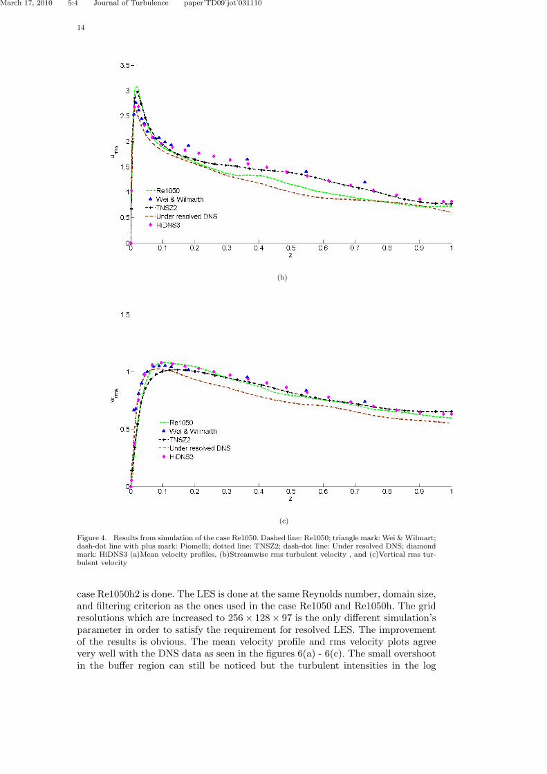
The second test case Re1050 is LES performed in a domain with the size 2.5π×0.5π×2, the resolution of 96×128×65 mesh points, at Re0 = 1050. The results forthis case are plotted in figures 4 together with the experimental results from Weiand Wilmarth [21], the DNS results from Del Alamo et al. [20], the LES resultsfrom Piomelli [22] obtained using the dynamic Smagorinsky model, the LES results


13

(a)

from Domaradzki et al. [3] obtained with the velocity estimation model (the caseTNSZ2), and the results from DNS without any modeling but at the same lowresolution of 96 × 128 × 65 as in two LES cases. The filtering condition is set to0.007 and the filter is found to be activated every 350 to 620 time steps. Thestatistically steady state was reached after about 16000 time steps. All LES meanvelocity data, including the case Re1050, are shown in Fig. 4(a) and are in goodmutual agreement though they slightly overpredict the experimental data. Figure4(b) shows the plot of the streamwise rms velocity from simulation compared withother baseline cases. The agreement with the experimental data and the TNSZ2data is good between z = 0 and z = 0.2 but the quality of comparison deterioratesfor larger values of z. The vertical rms velocity LES data shown in Fig. 4(c) arein good agreement with the experiments throughout the entire domain. No resultsfor the spanwise velocity are presented here because the experimental data for thatvelocity were not available for comparisons.

The simulation case Re1050h is the LES performed in the same domain size as theone used in the Re1050 case but with different grid resolutions. The grid resolutionsfor Re1050h case are adjusted according to the suggested grid resolutions in [6]. Alsoas reported in Piomelli [22], the prediction of mean velocity profile, rms velocity,and high order statistic quantities depends on the grid resolutions in near wallregion. The figures 5(a) -5(c) show the plots obtained from the simulation in thisRe1050h case compared with the experimental and DNS data from the same sourcesas the reference data used in figures 4(a) - 4(c). The mean velocity profile shown infigure 5(a) improves. The improvement is even more noticeable in the rms velocityplots. The effective friction Reynolds number also express the improvement of thenear wall dynamics captured by the computational grids. However there is still theovershoot of the streamwise component of rms velocity in near wall region and theprediction of the wall normal component of the rms velocity in near wall region stillneeds improving. These shows the inadequacy of the grid resolutions to resolve thestructures in near wall area which are significant in turbulent energy production,and SGS’ interactions.

With the resolved LES’s grid resolution in consideration, the simulation in the


14

(b)

(c)

Figure 4. Results from simulation of the case Re1050. Dashed line: Re1050; triangle mark: Wei & Wilmart;dash-dot line with plus mark: Piomelli; dotted line: TNSZ2; dash-dot line: Under resolved DNS; diamondmark: HiDNS3 (a)Mean velocity profiles, (b)Streamwise rms turbulent velocity , and (c)Vertical rms tur-bulent velocity

case Re1050h2 is done. The LES is done at the same Reynolds number, domain size,and filtering criterion as the ones used in the case Re1050 and Re1050h. The gridresolutions which are increased to 256× 128× 97 is the only different simulation’sparameter in order to satisfy the requirement for resolved LES. The improvementof the results is obvious. The mean velocity profile and rms velocity plots agreevery well with the DNS data as seen in the figures 6(a) - 6(c). The small overshootin the buffer region can still be noticed but the turbulent intensities in the log


15

(a)

region are different from the intensities in the case Re1050 and Re1050h. Thereis no overshoot in near wall region for streamwise component of rms velocity andthe wall normal component of rms velocity agrees very well with DNS data. Thesedenote that the grid resolutions used in LES in Re1050h2 case is able to resolve thenear wall structures. The effective friction Reynolds number in LES of Re1050hand Re1050h2 cases also exhibit that the structures in near wall area are capturedby the computational grids.

The figures 7(a) - 7(d) show plots obtained in LES at Re0 = 2000, domain size2.5π×0.5π×2, and the resolution 96×96×211. The filtering criterion is set to 0.008and the filter turns on automatically every 620 to 980 time steps. The statisticallysteady state is reached after about 15000 time steps. The comparisons are madewith under resolved DNS and with the HiDNS2 case, which is fully resolved DNSof Hoyas and Jimenez [19] but in the larger domain 8π×3π×2. The mean velocityshowed in Fig. 7(a) is in excellent agreement with the high resolution DNS data.The quality of the prediction for the streamwise rms velocity presented in figure7(b) is lower. LES overpredicts the peak of the urms from the HiDNS2 case andunderpredicts DNS results in the range z > 200. The remaining two rms trubulentvelocity components are shown in figures 7(c) and exhibit much better agreementwith the DNS data.

In the last test case Re2000L, the LES performed at Re0 = 2000, domain size7.5π×3π×2, and the resolution 256×768×131. The resolutions in wall normal andspanwise direction lie in the resolved LES range. The grid resolution in spanwisedirection is intentionally chosen to resolve streaks’ spacing in near wall region. Themean velocity profile and the rms velocity plots from the data obtained in Re2000Lcase are shown in the figures 8(a) - 8(d). The mean velocity profile in figure 8(a)shows similar trend as seen in the mean velocity profile in Re180 case. The slopeof the profile changes in the buffer region and in the log region. When comparedwith the Re2000S case, the rms velocities in Re2000L case show improvements.


16

(b)

(c)

Figure 5. Results from simulation of the case Re1050h. Dashed line: Re1050h; triangle mark: Wei &Wilmart; dash-dot line with plus mark: Piomelli; dotted line: TNSZ2; dash-dot line: Under resolved DNS;diamond mark: HiDNS3 (a)Mean velocity profiles, (b)Streamwise rms turbulent velocity , and (c)Verticalrms turbulent velocity

5. Conclusions

The numerical code employed in this work uses spectral methods stabilized by aweak filter which allows it to run for all Reynolds numbers and resolutions con-sidered. Despite the simulations being stable the results from such runs do notcompare well with the baseline DNS and experimental data, as expected fromunder-resolved DNS. It is thus clear that beyond numerical stabilization techniques


17

(a)

additional turbulence modeling procedures are required to obtain physically cor-rect results in simulations that do not resolve all relevant scales of motion. We havepresented the LES model that utilizes the low-pass filtering operation as the onlymodeling tool. The entire procedure follows closely the previously developed TNSapproach which uses the filter periodically to modify smallest resolved scales. In thepresent TNS implementation the energy of these scales is monitored and the filteris turned on automatically whenever the energy exceeds a threshold defined by aspecific criterion. We have tested the model on the turbulent channel flow prob-lem at different Reynolds numbers and at different computational resolutions anddomain sizes. Satisfactory comparisons among TNS results and various referencecases have been obtained. In particular, the quality of the results is comparableto the previous TNS procedure which uses a fixed time interval for the filtering aswell as additional subgrid scale estimated velocity.

The results from Re180, Re1050h, and Re2000L cases show that the filters used inall of the numerical experiments reported in this paper actually could not provideenough dissipation when the turbulent energy production mechanism functionsproperly. When more small scales are included in the computational domain due tohigher grid resolutions, the turbulence energy is increased. As discussed in Piomelli[22], the structures in near wall region which is significant in turbulent energyproduction appear more diffused if the grid resolutions used in LES are inadequate.The results from Re1050 and Re2000S cases seem to agree well with the referencedata, especially with the data from velocity estimation method. However this comesfrom the fact that the inadequate grid resolutions result in partial turbulent energyproduction. The filtering which acts to dissipate accumulated energy seems to beworking quite well to supply dissipation in buffer region which is the region thatthe turbulent energy production peaks. In log region, the filtering seems to be toostrong because total dissipation dominates the existing turbulent energy producedby the coarse computational grids. The turbulent intensities in core of the flow arenot quite sufficient. In order to investigate the turbulent energy production anddissipation issues, the LES at Reynolds number equal to 1050 with the resolvedLES’s grid resolutions is performed in the Re1050h2 case. The results clearly show


18

(b)

(c)

Figure 6. Results from simulation of the case Re1050h2. Dashed line: Re1050h2; triangle mark: Wei &Wilmart; dash-dot line with plus mark: Piomelli; dotted line: TNSZ2; dash-dot line: Under resolved DNS;diamond mark: HiDNS3 (a)Mean velocity profiles, (b)Streamwise rms turbulent velocity , and (c)Verticalrms turbulent velocity

that the increase of turbulent energy production improves the status at the logregion and away from the wall as already seen in the results from Re1050h case. Inthe wall normal rms velocity plot, it shows that the increase in molecular dissipationdue to the added small scales complements the dissipation due to filtering andthe total dissipation balances the turbulent energy in this area. The overshootnoticed in streamwise rms velocity in Re1050 and Re1050h cases disappears andthe prediction of the vertical rms velocity in near wall region is very good. This


19

(a)

(b)

shows that, together with the grid resolutions in the level of wall resolved LES,the proposed TNS method performs very good jobs. As mentioned above, the gridresolutions employed in Re1050 and Re2000S cases are too coarse to resolve thenear wall structure resulting low turbulent energy production. Because of this, thefiltering with the filters used in this paper which can not provide enough dissipationcan provide enough energy dissipation to balance the turbulent energy production.Although, in the Re1050 and Re2000S cases, the near wall streaks are not resolved,the low order statistics which are of interest by many engineering applications, arepredicted reasonably well compared with the reference data.

The proposed TNS method show that even though there is no explicit SGSmodeling, the functions of the small scale are implicitly emulated by the filtering


20

(c)

(d)

Figure 7. Results from simulation of the case Re2000S. Dashed line: Re2000S; diamond mark: HiDNS2;dash-dot line: Under resolved DNS (a)Mean velocity profiles, (b)Streamwise rms turbulent velocity ,(c)Spanwise rms turbulent velocity, and (d)Vertical rms turbulent velocity

and the computational grids. From the results presented in this paper, one mayexpect to see the improvements in its performance if the computational grids canemulate the nonlinear interactions among SGS in the flow well and the filtering cansupply enough dissipation to balance the turbulent energy production locally. Thelow dissipation noticed from the results could be overcome by applying differentfilters or modifying the filters’ widths. The predictions are expected to improvefrom this modification. The lack of the back scatter due to the missing of theSGS’ interaction with large scales locally needs to be addressed to correct the


21

(a)

(b)

insufficient turbulent intensities in area away from the wall. From the results fromall test cases, it is obvious that the proposed TNS method need improvement andit can be improved. However the simplicity and flexibility of the method are thefactors that one should appreciated.

It is rather obvious that the filtering criterion will depend on the filter’s form.However, one may conjecture that TNS results should be independent of the filter’sform as long as the filter’s effect is to substantially attenuate small scales whileleaving the large scales unchanged and if the filtering criterion is derived for thespecific filter used. We will investigate the dependence of the model on the filterform in the subsequent work.


22 REFERENCES

(c)

(d)

Figure 8. Results from simulation of the case Re2000L. Dashed line: Re2000L; diamond mark: HiDNS2;dash-dot line: Under resolved DNS (a)Mean velocity profiles, (b)Streamwise rms turbulent velocity ,(c)Spanwise rms turbulent velocity, and (d)Vertical rms turbulent velocity

References

[1] J. Domaradzki, and N. Adams, Direct modeling of subgrid scales of turbulence in large eddy simula-tions, Journal of Turbulence 3:1 (2002), p. 1.

[2] J. Domaradzki, and E. Saiki, A subgrid-scale model based on the estimation of unresolved scales ofturbulence, Phys. Fluids 9 (1997), p. 2148.

[3] J. Domaradzki, K. Loh, and P. Yee, Large eddy simulation using the subgrid-scale estimation modeland truncated Navier-Stokes dynamics, Theor. Comput. Fluid Dyn. 15 (2002), p. 421.

[4] S. Stolz, N. Adams, and L. Kleiser, An approximate deconvolution model for large eddy simualtionwith application to incompressible wall-bounded flows, Phys. Fluids 13 pages =.


REFERENCES 23

[5] B. Kosovic, D. Pullin, and R. Samtaney, Subgrid-scale modeling for large eddy simulations of com-pressible turbulence, Phys. Fluids 14 (2002), p. 1511.

[6] F. Grinstein, L. Margolin, and W. Rider Implicit Large Eddy Simulation, Cambridge University Press,2007.

[7] J. Domaradzki, and K. Loh, the subgrid-scale estimation model in the physical space representation,Phys. Fluids 11 (1999), p. 2330.

[8] M. Visbal, and D. Rizzetta, Large-Eddy Simulation on General Geometries Using Compact Differ-encing and Filtering schmemes, AIAA 2002-0288 (2002).

[9] M. Visbal, and D. Rizzetta, Large-eddy simulation on curvilinear grids using compact differencingand filtering schemes, J. Fluids Eng. 124 (2002), pp. 836–847.

[10] C. Bogey, and C. Bailly, Large Eddy Simulations of transitional round jets: Influence of the Reynoldsnumber on flow development and energy dissipation, Phys. Fluids 18 (2006), p. 065101.

[11] P. Diamessis, J. Domaradzki, and J. Hesthaven, A spectral multidomain penalty method model forthe simulation of high Reynolds number localized incompressible stratified turbulence, J. Comp. Phys.202 (2005), p. 298.

[12] M. Minguez, R. Pasquetti, and E. Serre, Spectral vanishing viscosity stabilized LES of the Ahmedbody turbulent wake, Comm. Comput. Phys. 5 (2009), pp. 635–648.

[13] P. Diamessis, Y. Lin, and J. Domaradzki, Effective numerical viscosity in spectral multidomain penaltymethod-based simulations of localized turbulence, J. Comp. Phys. 227 (2008), pp. 8145–8164.

[14] H. Jeanmart, and G. Winckelmans, Investigation of eddy-viscosity models modified using discretefilters: A simplified Regularized variational multiscale model and on enhanced field model, Phys.Fluids 19 (2007).

[15] P. Yee, Ph.D. diss., University of Southern California, CA, 2000.[16] S. Gottlieb, and J. Hesthaven, Spectral methods for hyperbolic problems, J. Comput. Appl. Math 128

(2001), p. 83.[17] R. Kerr, Velocity, scalar and transfer spectra in numerical turbulence, J. Fluid Mech. 211 (1990), p.

309.[18] N. Gilbert, and L. Kleiser, Turbulence model testing with the aid of direct numerical simulation

results, in Proceedings of 8th Symposium on Turbulence shear flows, Munich, Germany, 1991.[19] S. Hoyas, and J. Jimenez, Scaling of the velocity fluctuations in Turbulence channels up to Reτ =

2003, Phys. Fluids 18 (2006).[20] J. Del Alamo, J. Jimenez, P. Zandonade, and R. Mozer, Scaling of the energy spectra of tuebulent

channels, J. Fluid Mech. 500 (2004), p. 135.[21] T. Wei, and W. Wilmarth, Reynolds number effects on the structure of Turbulent channel flow, J.

Fluid Mech. 204 (1989), p. 57.[22] U. Piomelli, High Reynolds number calculation using the dynamics subgrid scale model, Phys. Fluids

A5 (1993), p. 1484.

Truncated Navier-Stokes Equations with the Automatic Filtering

Documents

Transcript of Truncated Navier-Stokes Equations with the Automatic Filtering