A Finite Volume Solution of Unsteady Incompressible Navier ...

Corresponding author e-mail: [email protected] © 2019 NSP Natural Sciences Publishing Cor.

Num. Com. Meth. Sci. Eng. 1, No. 3, 117-131 (2019) 117

http://dx.doi.org/10.18576/ncmsel/010302

A Finite Volume Solution of Unsteady Incompressible Navier-Stokes Equations Using MATLAB

Endalew Getnet Tsega Department of Mathematics, College of Science, Bahir Dar University, Bahir Dar, Ethiopia Received: 2 Sep. 2019, Revised: 5 Oct. 2019, Accepted: 21 Oct. 2019. Published online: 1 Nov. 2019.

Abstract: Navier-Stokes equations which represent the momentum conservation of an incompressible Newtonian fluid flow are the fundamental governing equations in fluid dynamics. For real fluid flow situations, the equations are too difficult to solve analytically except for very simplified cases. A formal uniqueness and existence of the solutions has not been established using mathematical analysis. Nowadays, high speed and large memory computers have been used to solve the Navier-Stokes equations approximately together with continuity equations using a variety of numerical techniques. In this study, a finite volume technique is used to solve the Navier-Stokes equations for unsteady flow of Newtonian incompressible fluid with no body forces using MATLAB. The method is implemented on unsteady internal fluid flow in a 2D straight channel. The equations are solved to obtain velocity and pressure fields on staggered grid. The x and y velocity components are recomputed together at new locations to determine the resultant velocity at those locations. The computed velocity and pressure values using the solution method show a good agreement with that of the commercial CFD software, ANSYS Fluent. The solution method provides a possible alternative for handling resultant velocity and implementation of boundary conditions in discretization method by staggered grid. The result of this study can help users to write their own codes and use commercial CFD codes proficiently in solving equations of fluid flow using numerical discretization schemes. Keywords: Navier–Stokes equations; Finite volume method; 2D unsteady flow; Channel flow; Staggered grid; Numerical simulation; MATLAB 1 Introduction

The conservation of linear momentum for flow of incompressible Newtonian fluids is mathematically described by nonlinear partial differential equations known as Navier-Stokes equations. Solutions to the Navier–Stokes equations are used in many practical applications, for example, in engineering analysis and design, aerospace, pipe flow, open channel and river flow, industrial processes, weather prediction and biofluid dynamics [1, 2]. The exact solutions of the Navier Stokes equations for fluid flow are possible only for some simplified situations [3]. Thus, numerical methods are used to obtain solutions to Navier Stokes equations. They are solved jointly with continuity equation. The most widely used numerical methods employed are finite difference method (FDM), finite volume method (FVM) and finite element method (FEM) [4]. The accuracy of numerical methods depends on proper description of the physical models and boundary conditions incorporated in the governing equations [5]. For complex fluid flows, handling the corresponding governing equations is not easy. Therefore, numerical simulations should be supported with experimental tests for such cases [6].

FVM is one of the most popular numerical techniques to discritize the differential equations which describe fluid flow [1, 7, 8]. In FVM, the computational domain is discrtized into small subdomains called control volumes or cells on which flow variables are computed. The equations governing the fluid flow are integrated over the control volumes. By employing Divergence Theorem, the resulting volume integrals are transformed to surface integrals. The surface integrals are approximated in terms of variables defined at the adjacent grids. By this process, the governing differential equations are converted to algebraic equations to be solved by computers. Similar to FDM, values of flow variables in FVM are calculated at the discrete points on a computational domain. The FVM, like the FEM, has the ability of handling complex irregular computational domains. It can be implemented on structured and unstructured meshes. In FVM, conservation of governing equations is ensured at each finite volume [9]. These attributes have made the FVM appropriate for numerical simulation of fluid flow [8]. Majority of commercial computational fluid dynamics (CFD) codes today used FVM [1].

Numerical and Computational Methods in Sciences & Engineering An International Journal

118 E. G. Tsega: A finite volume solution of Navier-Stokes equations…

© 2019 NSP Natural Sciences Publishing Cor.

Many authors discussed the finite volume discretization of the governing equations of fluid flow over the computational domain using staggered grid [8, 10, 11, 12]. The staggered grid is a setting for the spatial discretization, in which the flow variables are not computed at the same position on the domain. Pressure is evaluated at nodes located at the centroid of the control volumes and the velocity components are calculated at the different grid points placed at the center of faces of the control volumes. This assignment gives a strong relationship between the velocities and pressure. This in turn helps to enhance convergence and to avoid oscillations of the velocity and pressure fields in the numerical computation [1].

The objective of this study is to obtain numerical solution of unsteady Navier-Stokes equations for incompressible Newtonian fluid flow using an in-house MATLAB code. To end this, the SIMPLE algorithm is employed on staggered grids. Boundary conditions are considered carefully in the discretization. The computed velocity components on staggered grid are in turn used to approximate the velocity components together at new locations to obtain the resultant velocity for numerical simulations.

2 Governing Equations

The equations which govern the incompressible Newtonian fluid flows are the continuity equation (conservation of mass) and Navier-Stokes equation (conservation of momentum). The equations in vector and dimensionless form are: Continuity Equation (1) Navier-Stokes Equation

(2)

where is the velocity and p is pressure at time t. The constant is the Reynolds number for the

flow ( is density of the fluid, is the dynamic viscosity of the fluid , and L represent the reference velocity and length scale) and is the del operator. A derivation of these governing equations can be found in [11]. Terms on the left side of Eq. (2) are transient and convective terms where as on the right we have pressure gradient and diffusive terms.

3 Finite Volume Discretization and Solution Procedure

After dividing a flow domain into control volumes, the continuity and Navier-Stokes equations are integrated over each

control volume to transform the equations to a system of algebraic equations relating the flow variables. The resulting

equations are solved in iterative manner. The finite volume discretizations of the equations on a control volume W are

explained in this section and for further detail see [11].

Integrating Eq.(1), over the control volume W (see Figure 1) , we get (3)

Applying Gauss’s Divergence Theorem, we have (4)

Here, S is the surface bounding W and n is the outward unit normal to S.

(5)

where f shows summation over face of each control volume. In Eq.(5), represents the average velocity at the face and

is value of velocity at the center of the face . is the outward unit normal to and is the area of the face . Hence, (6)

. =0Ñ v

( )1.( ) .( )Re

ptÑ Ñ Ñ Ñ¶+ = - +

¶v vv v

( , , )u v w=v Re VLrµ

=

r µ VÑ

. 0dW

Ñ W =òòò v

. 0S

dS =òòv n

. . . .f ff f fS S S S

dS dS A Aæ ö

= » »ç ÷è ø

å å åòò òò òò òòf f f fv n v n v n v n

fv f

fv f fn f fA f

. 0ff S

A =åòò f fv n

Num. Com. Meth. Sci. Eng. 1, No. 3, 117-131 (2019)/ http://www.naturalspublishing.com/Journals.asp 119


Integrating momentum equations, Eq.(2), over the control volume W, we get the following for momentum equations. Unsteady term

(7)

where DV is the volume of W. Convective terms

(8)

Pressure gradient term Applying Green-Gauss Theorem, we get (9)

Viscous terms

(10) From Eq.(2) and Eq.(7)-Eq.(10), we get

(11)

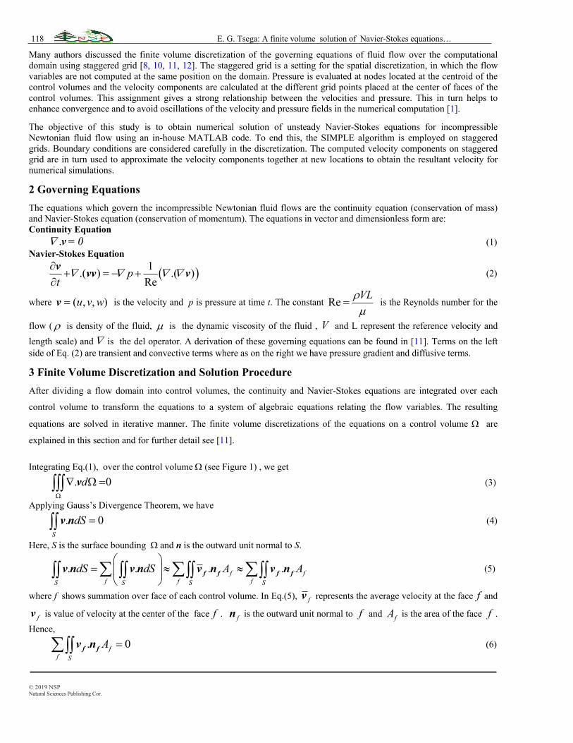
(a) (b)

Figure 1 (a) 2D control volume (b) 3D control volume.

In order to illustrate the finite volume solution procedure to solve fluid flow problems, let us consider unsteady internal fluid flow in a 2D straight channel (Figure 2) of length L and height H where the fluid is incompressible and Newtonian with constant density and viscosity.

d Vt tW

¶ ¶W = D

¶ ¶òòòv v

.( ) ( ). ( ). ( ) . ( ) .f f f f f ff f fS S

d dS dS A AW

æ öÑ W = = » »ç ÷

è øå å åòòò òò òòvv vv n vv n vv n vv n

( f f f f f ff f fS S

pd p dS p dS p A p AW

- Ñ W = - = - » - » -å å åòòò òò òòn n n n

1 1 1 1 1.( ) ( ). ( ) . ( ) . ( ) .Re Re Re Re Ref f f f f f f f

f f fS S

d dS dS A AW

æ öÑ Ñ W = Ñ = Ñ » Ñ » Ñç ÷

è øå å åòòò òò òòv v n v n v n v n

1( ) . ( ) .Ref f f f f f f f f

f f fV A p A A

t¶D + = - + Ñ

¶ å å åv vv n n v n



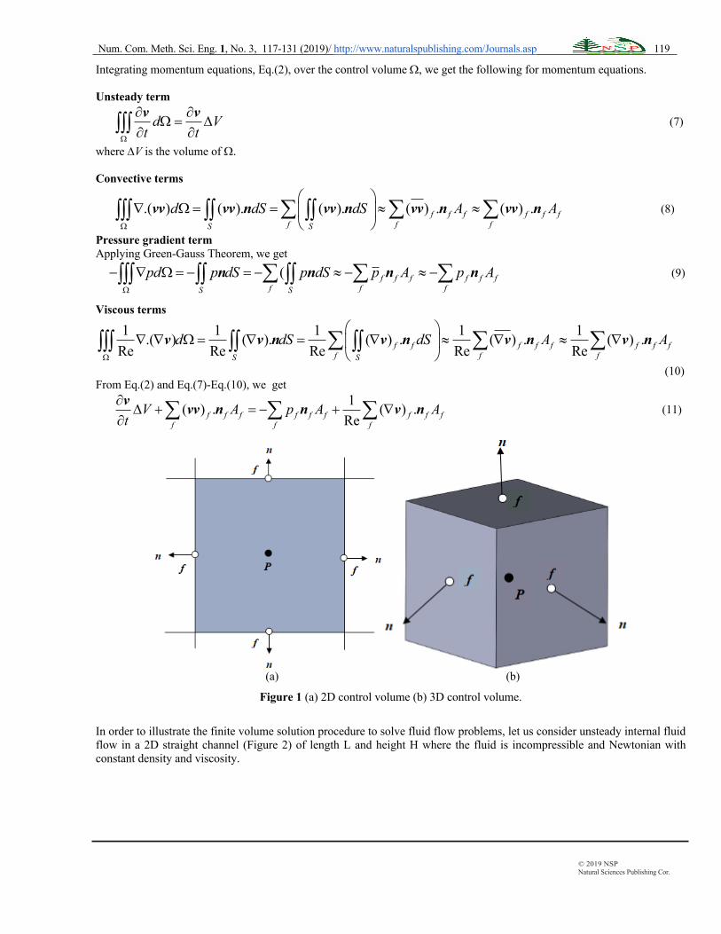
Figure 2 Schematic representation of internal fluid flow in a 2D straight channel.

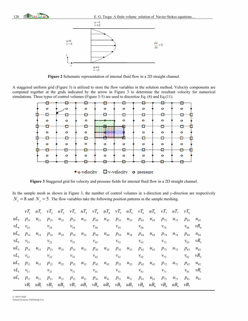
A staggered uniform grid (Figure 3) is utilized to store the flow variables in the solution method. Velocity components are computed together at the grids indicated by the arrow in Figure 3 to determine the resultant velocity for numerical simulations. Three types of control volumes (Figure 3-5) are used to discretize Eq. (6) and Eq.(11).

Figure 3 Staggered grid for velocity and pressure fields for internal fluid flow in a 2D straight channel.

In the sample mesh as shown in Figure 3, the number of control volumes in x-direction and y-direction are respectively

and . The flow variables take the following position patterns in the sample meshing.

8xN = 5yN =

1 1 2 2 3 3 4 4 5 5 6 6 7 7 8

5 15 15 25 25 35 35 45 45 55 55 65 65 75 75 85 85

4 14 24 34 44 54 64 74 84 4

4 14 14 24 24 34 34 44 44 54 54 64 64 74 74 84 84

3 13 23 33 43 53 63 7

vT uT vT uT vT uT vT uT vT uT vT uT vT uT vTuL p u p u p u p u p u p u p u p uvL v v v v v v v v vRuL p u p u p u p u p u p u p u p uvL v v v v v v v 3 83 3

3 13 13 23 23 33 33 42 42 52 52 62 62 72 72 82 82

2 12 22 32 42 52 62 72 82 2

2 12 12 22 22 32 32 42 42 52 52 62 62 72 72 82 82

1 11 21 31 41 51 61 71 81 1

1 11 11 21 21 31 31 41 41 51

v vRuL p u p u p u p u p u p u p u p uvL v v v v v v v v vRuL p u p u p u p u p u p u p u p uvL v v v v v v v v vRuL p u p u p u p u p u51 61 61 71 71 81 81

1 1 2 2 3 3 4 4 5 5 6 6 6 6 7

p u p u p uvB uB vB uB vB uB vB uB vB uB vB uB vB uB vB



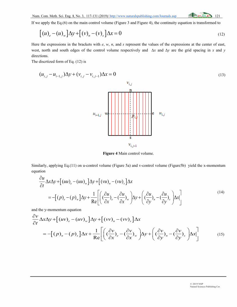
If we apply the Eq.(6) on the main control volume (Figure 3 and Figure 4), the continuity equation is transformed to

(12)

Here the expressions in the brackets with e, w, n, and s represent the values of the expressions at the center of east, west, north and south edges of the control volume respectively and Dx and Dy are the grid spacing in x and y directions. The discrtized form of Eq. (12) is

(13)

Figure 4 Main control volume.

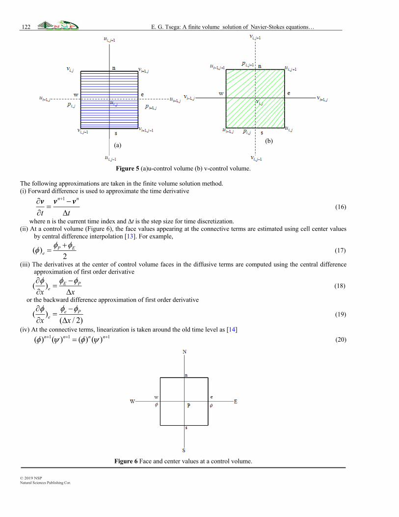
Similarly, applying Eq.(11) on u-control volume (Figure 5a) and v-control volume (Figure5b) yield the x-momentum equation

(14)

and the y-momentum equation

(15)

[ ] [ ]( ) ( ) ( ) ( ) 0e w n su u y v v x- D + - D =

, 1, , , 1( ) ( ) 0i j i j i j i ju u y v v x- -- D + - D =

[ ] [ ]

[ ]

( ) ( ) ( ) ( )

1( ) ( ) ( ) ( ) ( ) ( )Re

e w n s

e w e w n s

u x y uu uu y vu vu xt

u u u up p y y xx x y y

¶D D + - D + - D

¶é ùæ ö¶ ¶ ¶ ¶æ ö= - - D + - D + - Dê úç ÷ç ÷¶ ¶ ¶ ¶è ø è øë û

[ ] [ ]

[ ]

( ) ( ) ( ) ( )

1( ) ( ) ( ) ( ) ( ) ( )Re

e w n s

n s e w n s

v x y uv uv y vv vv xt

v v v vp p x y xx x y y

¶D D + - D + - D

¶é ùæ ö¶ ¶ ¶ ¶æ ö= - - D + - D + - Dê úç ÷ç ÷¶ ¶ ¶ ¶è ø è øë û



Figure 5 (a)u-control volume (b) v-control volume.

The following approximations are taken in the finite volume solution method. (i) Forward difference is used to approximate the time derivative

(16)

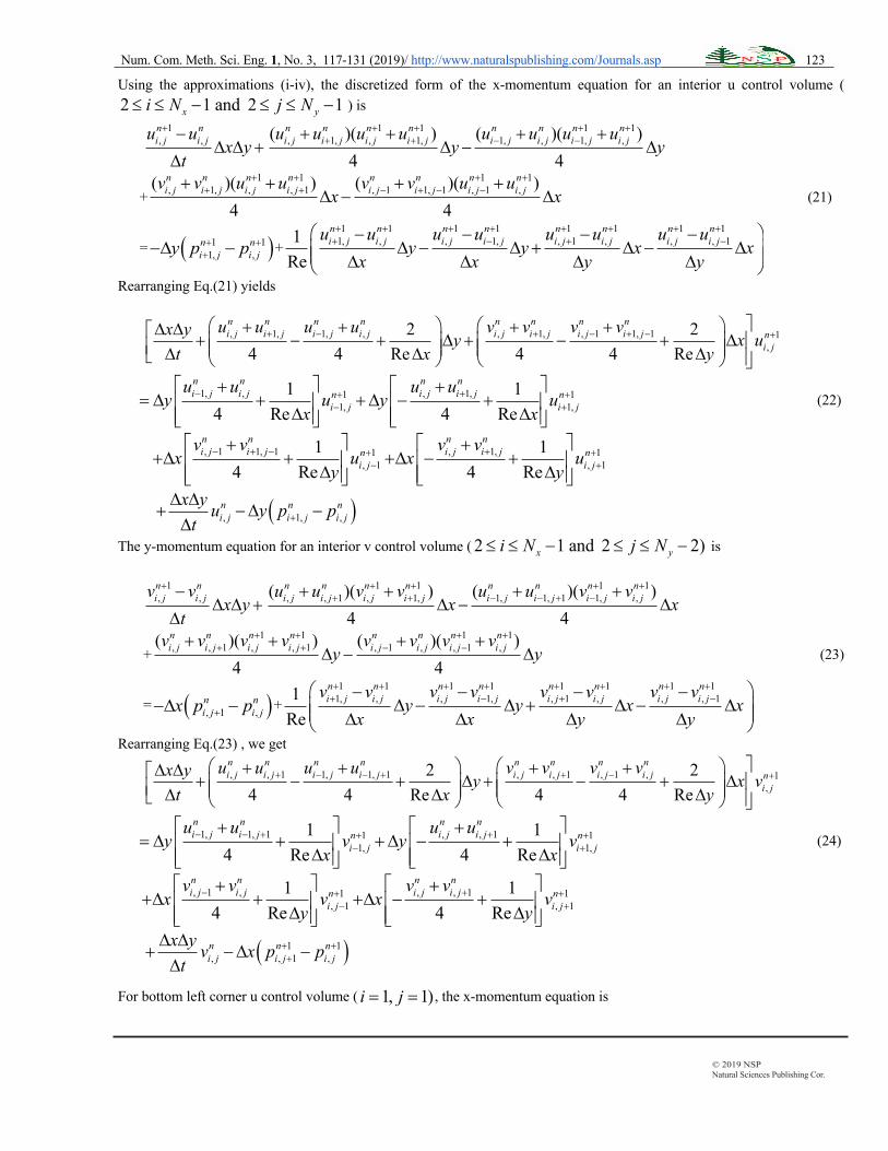
where n is the current time index and Dt is the step size for time discretization. (ii) At a control volume (Figure 6), the face values appearing at the connective terms are estimated using cell center values

by central difference interpolation [13]. For example,

(17)

(iii) The derivatives at the center of control volume faces in the diffusive terms are computed using the central difference approximation of first order derivative

(18)

or the backward difference approximation of first order derivative

(19)

(iv) At the connective terms, linearization is taken around the old time level as [14] (20)

Figure 6 Face and center values at a control volume.

1n n

t t

+¶ -=

¶ Dv v v

( )2

P Ee

f ff +=

( ) E Pex x

f ff -¶=

¶ D

( )( / 2)e P

ex xf ff -¶

=¶ D

1 1 1( ) ( ) ( ) ( )n n n nf y f y+ + +=

(a) (b)



Using the approximations (i-iv), the discretized form of the x-momentum equation for an interior u control volume ( ) is

+ (21)

= +

Rearranging Eq.(21) yields

(22)

The y-momentum equation for an interior v control volume ( is

+ (23)

= +

Rearranging Eq.(23) , we get

(24)

For bottom left corner u control volume ( , the x-momentum equation is

2 1 and 2 1x yi N j N£ £ - £ £ -1

, ,n ni j i ju u

x yt

+ -D D +

D

1 1 1 1, 1, , 1, 1, , 1, ,( )( ) ( )( )

4 4

n n n n n n n ni j i j i j i j i j i j i j i ju u u u u u u u

y y+ + + +

+ + - -+ + + +D - D

1 1 1 1, 1, , , 1 , 1 1, 1 , 1 ,( )( ) ( )( )

4 4

n n n n n n n ni j i j i j i j i j i j i j i jv v u u v v u u

x x+ + + +

+ + - + - -+ + + +D - D

( )1 11, ,n ni j i jy p p+ ++-D -

1 1 1 1 1 1 1 11, , , 1, , 1 , , , 11

Re

n n n n n n n ni j i j i j i j i j i j i j i ju u u u u u u u

y y x xx x y y

+ + + + + + + ++ - + -æ ö- - - -

D - D + D - Dç ÷ç ÷D D D Dè ø

, 1, 1, , , 1, , 1 1, 1 1,

2 24 4 Re 4 4 Re

n n n n n n n ni j i j i j i j i j i j i j i j n

i j

u u u u v v v vx y y x ut x y

+ - + - + - +ùæ ö æ ö+ + + +D Dé + - + D + - + D úç ÷ ç ÷ê ç ÷ ç ÷D D Dë úè ø è ø û

1, , , 1,1 11, 1,

1 14 Re 4 Re

n n n ni j i j i j i jn n

i j i j

u u u uy u y u

x x- ++ +

- +

é ù é ù+ += D + +D - +ê ú ê ú

D Dê ú ê úë û ë û

, 1 1, 1 1, 1

14 Re

n ni j i j n

i j

v vx u

y- + - +

-

é ù++D +ê ú

Dê úë û

, 1, 1, 1

14 Re

n ni j i j n

i j

v vx u

y+ +

+

é ù++D - +ê ú

Dê úë û

( ), 1, ,n n ni j i j i j

x y u y p pt +

D D+ -D -

D2 1 and 2 2)x yi N j N£ £ - £ £ -

1, ,n ni j i jv v

x yt

+ -D D +

D

1 1 1 1, , 1 , 1, 1, 1, 1 1, ,( )( ) ( )( )

4 4

n n n n n n n ni j i j i j i j i j i j i j i ju u v v u u v v

x x+ + + +

+ + - - + -+ + + +D - D

1 1 1 1, , 1 , , 1 , 1 , , 1 ,( )( ) ( )( )

4 4

n n n n n n n ni j i j i j i j i j i j i j i jv v v v v v v v

y y+ + + +

+ + - -+ + + +D - D

( ), 1 ,n ni j i jx p p+-D -

1 1 1 1 1 1 1 11, , , 1, , 1 , , , 11

Re

n n n n n n n ni j i j i j i j i j i j i j i jv v v v v v v v

y y x xx x y y

+ + + + + + + ++ - + -æ ö- - - -


, , 1 1, 1, 1 , , 1 , 1 , 1,

2 24 4 Re 4 4 Re

n n n n n n n ni j i j i j i j i j i j i j i j n

i j

u u u u v v v vx y y x vt x y

+ - - + + - +ùæ ö æ ö+ + + +D Dé + - + D + - + D úç ÷ ç ÷ê ç ÷ ç ÷D D Dë úè ø è ø û

1, 1, 1 , , 11 11, 1,

1 14 Re 4 Re


i j i j

u u u uy v y v

x x- - + ++ +

- +

é ù é ù+ += D + +D - +ê ú ê ú


, 1 , 1, 1

14 Re

n ni j i j n

i j

v vx v

y- +

-

é ù++D +ê ú

Dê úë û

, , 1 1, 1

14 Re

n ni j i j n

i j

v vx v

y+ +

+

é ù++D - +ê ú

Dê úë û

( )1 1, , 1 ,n n ni j i j i j

x y v x p pt

+ ++

D D+ -D -

D

1, 1)i j= =



+ (25)

= +

Note that the derivative at the center of south face of the volume is approximated using the backward difference scheme. Eq. (25) can be written as

(26)

+ +

+

The x-momentum equations for bottom right corner ( , top left corner and top right corner

( u control volumes can be obtained in similar way.

For left boundary u control volume ( , the x-momentum equation is

+ (27)

= +

Eq. (28) can be written as

(28)

+ +

The momentum equations for remaining boundary u control volumes and corner and boundary v control volumes can be formulated analogously.

The resulting system of continuity and momentum equations for the finite volume discretization is solved with SIMPLE

1, ,n ni j i ju u

x yt

+ -D D +

D

1 1 1, 1, , 1, , ,( )( ) ( ( ) )( ( ) )

4 4

n n n n n ni j i j i j i j i j i ju u u u uL j u uL j u

y y+ + +

+ ++ + + +D - D

1 1, 1, , , 1( )( ) ( ( ) ( 1)) ( )

4 2

n n n ni j i j i j i jv v u u vB i vB ix uB i x

+ ++ ++ + + +

D - D

( )1 11, ,n ni j i jy p p+ ++-D -

1 1 1 1 1 11, , , , 1 , ,( ) ( )1

Re ( / 2)

n n n n n ni j i j i j i j i j i ju u u uL j u u u uB i

y y x xx x y y

+ + + + + ++ +æ ö- - - -


, 1, , , 1, 1,

( )( ( ) ) 2 34 4 Re 4 Re

n n n n ni j i j i j i j i j n

i j

u u uL j uL j u v vx y y x ut x y

+ + +ùæ ö æ ö+ + +D Dé + - + D + + D úç ÷ ç ÷ê ç ÷ ç ÷D D Dë úè ø è ø û

, 1, , 1,1 11, , 1

1 14 Re 4 Re


i j i j

u u v vy u x u

x y+ ++ +

+ +

é ù é ù+ += D - + +D - +ê ú ê ú


( ), 1, ,n n ni j i j i j

x y u y p pt +

D D+ -D -

D,( )( ( ) )

4

ni juL j uL j u

y+

D( ( ) ( 1)) ( )

2vB i vB i uB i y+ +

D

1 2( ) ( )Re Re

y xuL j uB ix y

D D+

D D1, 1)xi N j= - = 1, )yi j N= =

1, )x yi N j N= - =

1, 2 1, )yi j N= £ £ -1

, ,n ni j i ju u

x yt

+ -D D +

D

1 1 1, 1, , 1, , ,( )( ) ( ( ) )( ( ) )

4 4

n n n n n ni j i j i j i j i j i ju u u u uL j u uL j u

y y+ + +

+ ++ + + +D - D

1 1 1 1, 1, , , 1 , 1 1, 1 , 1 ,( )( ) ( )( )

4 4

n n n n n n n ni j i j i j i j i j i j i j i jv v u u v v u u

x x+ + + +

+ + - + - -+ + + +D - D

( )1 11, ,n ni j i jy p p+ ++-D -

1 1 1 1 1 1 11, , , , 1 , , , 1( )1

Re

n n n n n n ni j i j i j i j i j i j i ju u u uL j u u u u

y y x xx x y y

+ + + + + + ++ + -æ ö- - - -


, 1, , , 1, , 1 1, 1 1,

( )( ( ) ) 2 24 4 Re 4 4 Re

n n n n n n ni j i j i j i j i j i j i j n

i j

u u uL j uL j u v v v vx y y x ut x x

+ + - + - +ùæ ö æ ö+ + + +D Dé + - + D + - + D úç ÷ ç ÷ê ç ÷ ç ÷D D Dë úè ø è ø û

, 1, 11,

14 Re

n ni j i j n

i j

u uy u

x+ +

+

é ù+= D - +ê ú

Dê úë û

, 1 1, 1 1, 1

14 Re

n ni j i j n

i j

v vx u

y- + - +

-

é ù++D +ê ú

Dê úë û

, 1, 1, 1

14 Re

n ni j i j n

i j

v vx u

y+ +

+

é ù++D - +ê ú

Dê úë û

( ), 1, ,n n ni j i j i j

x y u y p pt +

D D+ -D -

D,( )( ( ) )

4

ni juL j uL j u

y+

D1 ( )Re

yuL jx

DD



algorithm. Here, the algorithm is presented using equations obtained from the interior control volumes. First we have to guess initial values of the velocity fields , and pressure field . Eq. (22) and Eq. (24) are solved to obtain

the values of and . The velocity fields and obtained do not satisfy the continuity equation, Eq. (13). Assume that we can find velocity corrections and that adjusts the velocity fields so that they satisfy the continuity equation. Then

(29)

(30)

where and are the velocity components that satisfy the continuity equation. For the velocity corrections, a pressure correction is required so that

(31)

In order to obtain , Eq. (22) is approximated as

(32)

In order to obtain , Eq. (24) is approximated as

(33)

To compute the value of using Eq. (33), the values of computed in Eq. (32) are used immediately.

Neglecting terms containing the neighbours , , and of , using the guessed values , for nth values in Eq.(22) and subtracting Eq. (32) from Eq. (22), we get

nu )( * nv )( * np )( *1)( +* nu 1)( +* nv 1)( +* nu 1)( +* nv

'u 'v

')( 11 uuu nn +*= ++

')( 11 vvv nn +*= ++

1+nu 1+nv'p

')(1 ppp nn +*=+

1)( +* nu

, 1, 1, ,

, 1, , 1 1, 1 1,

( *) ( *) ( *) ( *) 24 4 Re

( *) ( *) ( *) ( *) 2 ( *)4 4 Re

n n n ni j i j i j i j

n n n ni j i j i j i j n

i j

u u u ux y yt x

v v v vx u

y

+ -

+ - + - +

æ ö+ +D Dé + - + Dç ÷ê ç ÷D Dë è øùæ ö+ +

+ - + D úç ÷ç ÷D úè ø û

1, , , 1,1 11, 1,

( *) ( *) ( *) ( *)1 1( *) ( *)4 Re 4 Re


i j i j

u u u uy u y u

x x- ++ +

- +

é ù é ù+ += D + +D - +ê ú ê ú


, 1 1, 1 1, 1

( *) ( *) 1 ( *)4 Re

n ni j i j n

i j

v vx u

y- + - +

-

é ù++D +ê ú

Dê úë û

, 1, 1, 1

( *) ( *) 1 ( *)4 Re

n ni j i j n

i j

v vx u

y+ +

+

é ù++D - +ê ú

Dê úë û

( ), 1, ,( *) ( *) ( *)n n ni j i j i j

x y u y p pt +

D D+ -D -

D1)( +* nv

, , 1 1, 1, 1

, , 1 , 1 , 1,

( *) ( *) ( *) ( *) 24 4 Re

( *) ( *) ( *) ( *) 2 ( *)4 4 Re


n n n ni j i j i j i j n

i j

u u u ux y yt x

v v v vx v

y

+ - - +

+ - +

æ ö+ +D Dé + - + Dç ÷ê ç ÷D Dë è øùæ ö+ +

+ - + D úç ÷ç ÷D úè ø û1, 1, 1 , , 11 1

1, 1,

( *) ( *) ( *) ( *)1 1( *) ( *)4 Re 4 Re


i j i j

u u u uy v y v

x x- - + ++ +

- +

é ù é ù+ += D + +D - +ê ú ê ú


, 1 , 1, 1

( *) ( *) 1 ( *)4 Re

n ni j i j n

i j

v vx v

y- +

-

é ù++D +ê ú

Dê úë û

, , 1 1, 1

( *) ( *) 1 ( *)4 Re

n ni j i j n

i j

v vx v

y+ +

+

é ù++D - +ê ú

Dê úë û

( )1 1, , 1 ,( *) ( *) ( *)n n ni j i j i j

x y v x p pt

+ ++

D D+ -D -

D1)( +* nv 1)( +* nu

jiu ,1- 1,i ju + , 1i ju - , 1i ju + jiu ,nu )( * nv )( *



(34)

where

From Eq. (34), we get (35)

where

From Eq. (29) and Eq. (35), we get (36)

Neglecting terms containing the neighbours , , , and of , using the guessed values , for nth values in Eq.(24) and subtracting Eq. (33) from Eq. (24), we get (37)

where

+

Eq. (37) leads to (38)

where

From Eq. (30) and Eq.(38), we have (39)

Eq. (36) and Eq.(39) are called velocity correction equations. Using Eq. (36) and Eq. (39) in Eq. (13), we get

(40)

+

From Eq. (40), we get the pressure correction equation

+ (41)

From Eq. (31) and Eq.(41), we get

( )', , 1, ,i j i j i j i jax u y p p+¢ ¢= -D -

, 1, 1, 1, 1,

, 1, , 1 1, 1

( *) ( *) ( *) ( *) 24 4 Re

( *) ( *) ( *) ( *) 24 4 Re


i j


u u u ux yax yt x

v v v vx

y

+ - - +

+ - + -

æ ö+ +D D= + - + Dç ÷ç ÷D Dè øæ ö+ +

+ - + Dç ÷ç ÷Dè ø

=', jiu ( ), 1, ,i j i j i jDx p p+¢ ¢- -

,,

i ji j

yDxaxD

=

( )1 * 1, , , 1, ,( )n ni j i j i j i j i ju u Dx p p+ +

+¢ ¢= - -

jiv ,1- jiv ,1+ 1, -jiv 1, +jiv jiv ,nu )( * nv )( *

( )', , , 1 ,i j i j i j i jay v x p p+¢ ¢= -D -

, , 1 1, 1, 1( *) ( *) ( *) ( *) 24 4 Re

n n n ni j i j i j i ju u u ux y y

t x+ - - +æ ö+ +D D

+ - + Dç ÷ç ÷D Dè ø

, , 1 , 1 ,( *) ( *) ( *) ( *) 24 4 Re

n n n ni j i j i j i jv v v v

xy

+ -æ ö+ +- + Dç ÷ç ÷Dè ø

=', jiv ( ), , 1 ,i j i j i jDy p p+¢ ¢- -

,,

i ji j

xDyayD

=

( )1 * 1, , , , 1 ,( )n ni j i j i j i j i jv v Dy p p+ +

+¢ ¢= - -

( ) ( )( )( )* 1 * 1, , 1, , 1, 1, , 1,( ) ( ) .n ni j i j i j i j i j i j i j i ju Dx p p u Dx p p y+ +

+ - - -¢ ¢ ¢ ¢- - - - - D

( ) ( )( )( )* 1 * 1, , , 1 , , 1 , 1 , , 1( ) ( ) 0n ni j i j i j i j i j i j i j i jv Dy p p v Dy p p x+ +

+ - - -¢ ¢ ¢ ¢- - - - - D =

( ) ( )* 1 * 1 * 1 * 1, 1, , , 1 ,( ) ( ) ( ) ( )n n n ni j i j i j i j i jp y u u x v v+ + + +

- -é¢ = D - +D -ë

( ) ( ), 1, 1, 1, , , 1 , 1 , 1i j i j i j i j i j i j i j i jy Dx p Dx p x Dy p Dy p+ - - + - -ù¢ ¢ ¢ ¢D + +D + û

( ) ( ), 1, , , 1/ i j i j i j i jy Dx Dx x Dy Dy- -é ùD + +D +ë û



(42)

The finite volume solution procedures discussed so far can be summarized as follows. 1. Take initial guesses (u*)n, (v*)n and (p*)n . 2. Solve the momentum equations for (u*)n+1 and (v*)n+1 using Eq.(32) and Eq.(33). 3. Compute the pressure correction p’ using Eq. (42). 4. Compute velocity corrections u’ and v’ using Eq.(35) and Eq.(38). 5. Correct velocity components and pressure using Eq. (36), Eq.(39) and Eq.(42). 6. Calculate the velocity components together at new locations using the velocity components obtained in step 5. 7. Check the convergence. If convergence is satisfied, then stop and take solutions in step 6. Otherwise update the initial

guesses by using the results in step 5 and continue the process.

4 Numerical Simulations

A MATLAB code is developed to employ the finite volume method discussed so far to simulate fluid flow in 2D straight channel of Length and height . 100´50 square finite volume cells of grid size 0.01m are taken for simulation (Figure 5). The inlet flow velocity is taken to be 1m/s ( see Figure 2) and the Reynolds number of the flow is

( , ). For the outlet boundary condition, the flow is assumed to fully developed, the velocity distribution change close to the exit is very small, y-velocity is zero at the exit and the x-velocity at

nodes close to the exit is assigned to that at the exit nodes. The first order derivatives at the face centers of top and

bottom boundary u control volumes and at the face centers of left and right boundary v control volumes resulting

from the finite volume discretization of viscous terms are computed by backward difference approximation. The other derivatives are estimated using central difference approximation. Gauss-Seidel iterative method is used to solve the resulting system of momentum equations mentioned in step 2. The x-velocity component (u) and y-velocity component (v) are determined at each vertex of the main control volume to compute the resultant velocity at the vertices. At a vertex, the x-velocity component is computed by taking the average of the nearest top and bottom u velocity values and the y-velocity component by taking averages of the nearest left and right v velocity values which are obtained from computations using the staggered grid employing step 1-7. A time step size is used for the numerical solution. The convergence criteria is taken to be the summation of errors of the velocity components and is set as .

5 Results and Discussion

The computational methodology using the finite volume discretization presented in this study is validated with the finite element method (FEM) [15], Ghia et al. [16] and ANSYS Fluent 15 solutions for lid-driven cavity flow. The velocity components at the centroid of the lid-driven cavity flow for three solutions are illustrated in Table 1. It is observed that the solution using the finite volume method is in good agreement with that of FEM, Ghia et al. and ANSYS Fluent. Table 1. Comparison of results for velocity components at the geometric center of lid-driven cavity flow, Re =100.

Solution method Cells used x-velocity(m/s) y-velocity(m/s)

FVM with present MATLAB code 50x50 -0.2070 0.0574

FEM with a MATLAB code [14] 50x50 -0.2015 0.0568

ANSYS Fluent 50x50 -0.20808 0.056825

Ghia et al.[13] 129x129 -0.20581 0.05454

1 *, , ,( )n ni j i j i jp p p+ ¢= +

1L m= 0.5H m=

Re 100= 31 /kg mr = 0.01 / ( . )kg m sµ =

,( )n suy¶¶

,( )e wvx¶¶

v

0.005tD =610-



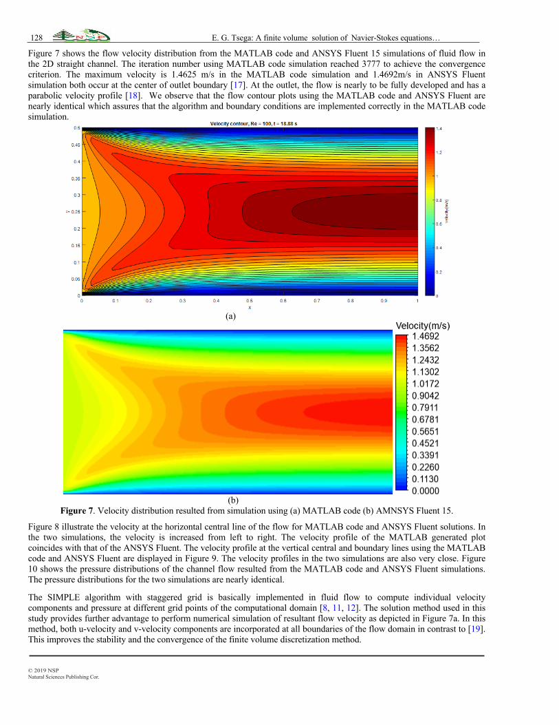
Figure 7 shows the flow velocity distribution from the MATLAB code and ANSYS Fluent 15 simulations of fluid flow in the 2D straight channel. The iteration number using MATLAB code simulation reached 3777 to achieve the convergence criterion. The maximum velocity is 1.4625 m/s in the MATLAB code simulation and 1.4692m/s in ANSYS Fluent simulation both occur at the center of outlet boundary [17]. At the outlet, the flow is nearly to be fully developed and has a parabolic velocity profile [18]. We observe that the flow contour plots using the MATLAB code and ANSYS Fluent are nearly identical which assures that the algorithm and boundary conditions are implemented correctly in the MATLAB code simulation.

(a)

(b)

Figure 7. Velocity distribution resulted from simulation using (a) MATLAB code (b) AMNSYS Fluent 15.

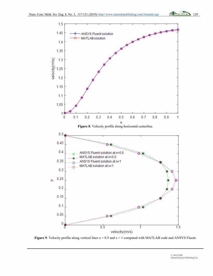
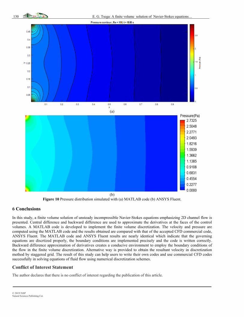
Figure 8 illustrate the velocity at the horizontal central line of the flow for MATLAB code and ANSYS Fluent solutions. In the two simulations, the velocity is increased from left to right. The velocity profile of the MATLAB generated plot coincides with that of the ANSYS Fluent. The velocity profile at the vertical central and boundary lines using the MATLAB code and ANSYS Fluent are displayed in Figure 9. The velocity profiles in the two simulations are also very close. Figure 10 shows the pressure distributions of the channel flow resulted from the MATLAB code and ANSYS Fluent simulations. The pressure distributions for the two simulations are nearly identical.

The SIMPLE algorithm with staggered grid is basically implemented in fluid flow to compute individual velocity components and pressure at different grid points of the computational domain [8, 11, 12]. The solution method used in this study provides further advantage to perform numerical simulation of resultant flow velocity as depicted in Figure 7a. In this method, both u-velocity and v-velocity components are incorporated at all boundaries of the flow domain in contrast to [19]. This improves the stability and the convergence of the finite volume discretization method.



Figure 8. Velocity profile along horizontal centerline.

Figure 9. Velocity profile along vertical lines x = 0.5 and x = 1 computed with MATLAB code and ANSYS Fluent.



(a)

(b)

Figure 10 Pressure distribution simulated with (a) MATLAB code (b) ANSYS Fluent. 6 Conclusions In this study, a finite volume solution of unsteady incompressible Navier-Stokes equations emphasizing 2D channel flow is presented. Central difference and backward difference are used to approximate the derivatives at the faces of the control volumes. A MATLAB code is developed to implement the finite volume discretization. The velocity and pressure are computed using the MATLAB code and the results obtained are compared with that of the accepted CFD commercial code, ANSYS Fluent. The MATLAB code and ANSYS Fluent results are nearly identical which indicate that the governing equations are discrtized properly, the boundary conditions are implemented precisely and the code is written correctly. Backward difference approximation of derivatives creates a conducive environment to employ the boundary conditions of the flow in the finite volume discretization. Alternative way is provided to obtain the resultant velocity in discretization method by staggered grid. The result of this study can help users to write their own codes and use commercial CFD codes successfully in solving equations of fluid flow using numerical discretization schemes.

Conflict of Interest Statement

The author declares that there is no conflict of interest regarding the publication of this article.



References

[1] J. Tu, G. H. Yeoh, C. Liu, Computational Fluid Dynamics: A Practical Approach. Butterworth-Heinemann, UK, pp.1-210, 2018.

[2] B. Xia, D. W. Sun, Applications of computational fluid dynamics (CFD) in the food industry: a review. Computers and Electronics in Agriculture 34, 5-24, 2002.

[3] H. Schlichting, K. Gersten, Exact Solution of Navier-Stokes Equations. In Boundary Layer Theory. Springer Berlin, Heidelberg, pp.101-142, 2017.

[4] J. H. Ferziger, Computational Methods for Fluid Dynamics. Third Edition, Springer-Verlag, New York, .pp.21-129, 2002.

[5] J. F. Wendt(Ed), Computational Fluid Dynamics: An Introduction. Third edition, Springer, Berlin, 2009.

[6] R. W. Johnson, The Handbook of Fluid Dynamics., Second edition, CRC Press , Boca Raton, 2016. [7] P. J. Zwart, G. D. Raithby, M. J. Raw, The integrated space-time finite volume method and its application to moving boundary

problems. Journal of Computational Physics 154, 497–519, 1999.

[8] H. K. Versteeg, W. Malalasekeraand, An Introduction to Computational Fluid Dynamics: The Finite Volume Method, Second edition, Prentice Hall, USA, 2007.

[9] A. Shukla, A. K. Singh, P. Singh , A comparative Study of Finite Volume Method and Finite difference Method for convection-Diffusion Problem, American Journal of Computational and Applied mathematics, 1(2), 67-73, 2011.

[10] F. H. Harlow, J. E. Welch, Numerical calculation of time dependent viscous incompressible flow with free surface. Physics of Fluids 8, 2182-2189, 1965.

[11] F. Moukalled, L. Mangani, M. Darwish, The Finite Volume Method in Computational Fluid Dynamics: An Advanced Introduction with OpenFOAM and Matlab, Springer, Switzerland, 2015.

[12] S. V. Patankar, Numerical Heat Transfer and Fluid Flow. Hemisphere, Washington D.C., 1980.

[13] W. Shyy, R. Mittal, Solution methods for the incompressible Navier-Stokes equations. In: R.W. Johnson(Ed), Handbook of Fluid Dynamics. Second Edition, CRC Press, Boca Roton, pp.1206-1227, 2016.

[14] J. H. Ferziger, M. Peric, Computational Methods for Fluid Dynamics. Third rev. Edition, Springer, Berlin, pp.116-206, 2002.

[15] E.G. Tsega, V. K. Katiyar, Finite Element Solution of the Two-dimensional Incompressible Navier-Stokes Equations Using MATLAB. Applications and Applied Mathematics: An International Journal (AAM) 13, 535-565, 2018.

[16] U. Ghia, K. N. Ghia, C. T. Shin, High-Re solutions for incompressible flow using the Navier-Stokes equations and a multigrid method. Journal of Computational Physics 48, 387-411, 1982.

[17] J. C. A. Hostos, V. D. Fachinotti, A. J. S. Pina, A. D. Bencomo, E. S. P. Cabrera, Implementation of standard penalty procedures for the solution of incompressible Navier-Stokes equations, employing the element-free Galerkin method. Engineering Analysis with Boundary Elements, DOI: 10.1016/j.enganabound.2018.08.008, 2018.

[18] F.M. White, Fluid Mechanics. Fifth Edition, McGraw Hill, New York, pp.258-261, 2003.

[19] V. Ambethkar, M .K. Srivastava, Numerical solutions of a steady 2-D incompressible flow in a rectangular domain with wall slip boundary conditions using the finite volume method. Journal of Applied Mathematics and Computational Mechanics 16(2), 5-16, 2017.

A Finite Volume Solution of Unsteady Incompressible Navier ...

Documents

Transcript of A Finite Volume Solution of Unsteady Incompressible Navier ...