This is the Final Submitted paper.

Please cite it as:

Rajeev Kumar and Brian H. Dennis. Unsteady incompressible flow computations with

least-squares/Galerkin split finite element method. ASME Early Career Technical

Conference hosted by ASME District E, Arlington, TX, USA, April 17 - 18, 2009.

2009 ECTC Proceedings ASME Early Career Technical Conference

Hosted by ASME District E April 17-18, 2009, Arlington, TX

UNSTEADY INCOMPRESSIBLE FLOW COMPUTATIONS WITH LEAST SQUARES/GALERKIN SPLIT FINITE ELEMENT METHOD

Rajeev Kumar1

Department of Mechanicaland Aerospace Engineering UTA Box 19018

The University of Texas at Arlington Arlington, TX 76019

rajeevkhp@yahoo.com

Brian H. Dennis2

Department of Mechanicaland Aerospace Engineering UTA Box 19018

The University of Texas at Arlington Arlington, TX 76019 dennisb@uta.edu

1 Post-Doc Researcher, Student member ASME 2 Assistant Professor, Member ASME

ABSTRACT The least squares finite element method (LSFEM) which

is based minimizing the l2-norm of the residuals is regarded as

an alternative approach to the well known Galerkin finite element methods (GFEM). In a variational setting, the LSFEM, unlike GFEM leads to minimization problem where compatibility conditions between approximation spaces like the restrictive LBB condition never arises and the resulting linear algebraic system has a symmetric positive definite matrix. However, the higher continuity requirements for second-order terms in the governing equations force the introduction of additional unknowns through the use of an equivalent first-order system of equations or the use of C

1

continuous basis functions. These additional unknowns lead to increased memory and computing time requirements that have limited the application of LSFEM to large-scale practical problems, such as three-dimensional compressible viscous flows. A novel finite element method is proposed that employs a least-squares method for first-order derivatives and a Galerkin method for second order derivatives, thereby avoiding the need for additional unknowns required by a pure LSFEM approach. When the unsteady form of the governing equations is used, a streamline upwinding term is introduced naturally by the least-squares method. Resulting system matrix is always symmetric and positive definite and can be solved by iterative solvers like pre-conditioned conjugate gradient method. The method is stable for convection-dominated flows and allows for equal-order basis functions for both pressure and velocity. The stability and accuracy of the method are demonstrated with results of several unsteady incompressible viscous flow benchmark problems solved using low-order C

0

continuous elements.

INTRODUCTION Since its introduction into fluid mechanics in early 70s,

finite element methods have gained popularity among computational community for solving fluid dynamic problems. Finite element methods developed for incompressible viscous

flows over the past few decades are mostly based on the velocity-pressure formulation. Examples of these methods are the segregated method, the penalty method, the mixed Galerkin method and least-squares method.

The segregated method [1, 2] employs a well known SIMPLE-type finite difference algorithm. Considerable computational efficiency can be obtained due to decoupling of velocity and pressure iterations, however due to lack of correct pressure boundary conditions for the pressure correction equation; the computed pressure is often inaccurate. In penalty method, the pressure is pre-eliminated by penalizing the continuity equation and recovered by using the perturbed conservation of mass equation [3HugesTJR].The penalty parameter affects the accuracy and convergence of the solution.

The classical mixed Galerkin method [4] is restricted by Ladyzhenskaya-Babuska-Brezzi (LBB) condition for the existence of the solution [5, 6]. The different basis functions used for the velocity and pressure in order to satisfy the LBB condition can be difficult to determine and implement. Also the system matrices turn out to be asymmetric and indefinite, which rules out the use of iterative methods to directly solve the system of equations.

In the past few years finite element models based on the least-squares variational principles have drawn considerable attention as an alternative approach [7-11]. The LSFEM has many attractive advantages over GFEM, notable among them is the lack of restrictive LBB condition and the resulting symmetric positive definite matrix system. However unlike the GFEM, where the continuity requirements of the finite element spaces are weakened by the integration by parts, LSFEM have associated with them the requirement of higher order continuity of the basis functions. This higher continuity requirement forces the introduction of additional unknowns by use of an equivalent first order system of equations or the use of C

1 continuous basis functions. These additional unknowns

lead to increased memory and computational requirements and overall the higher continuity requirement is generally

considered as a major drawback of the LSFEM which has limited its application to large scale practical problems such as 3D compressive viscous flows. A novel finite element approach that employs a least-squares method for first-order derivatives and a Galerkin method for second order derivatives, thereby avoiding the need for additional unknowns required by a pure LSFEM approach is presented in this work. Only the primitive variables u, v and p need to be solved for, in the two dimensional problems using the proposed method whereas LSFEM needs one additional unknown that is introduced in order to get the equivalent first order system [8, 9, 10]. In three dimensions LSFEM would require three additional unknowns whereas the proposed method still requires only the primitive variables. This is one of the attractive features of the proposed method. We call this method Least-Squares Galerkin Split finite element method (LSGSFEM). When the unsteady form of the governing equations is used, a streamline upwinding term is introduced naturally by the least-squares method. The method is stable for convection-dominated flows and allows for equal-order basis functions for both pressure and velocity. In addition, the resulting system of equations is always symmetric and is solved using the conjugate gradient method with standard pre-conditioners.

Non-linear terms are treated effectively by linearization in time. The stability and accuracy of the method are demonstrated with results of few unsteady incompressible viscous flow problems solved using low-order C

0 continuous

elements.

NOMENCLATURE u, v x,y velocity components respectively

U free-stream velocity p pressure C

i continuity of basis function

C solute concentration C0 initial solute concentration f frequency of vortex shedding d diameter or reference length

µ/, kinematic viscocity

Re UL/, Reynolds number

St fd/U, Strouhal number SIMPLE Semi-Implicit Method for Pressure Linked

Equations

UNSTEADY LSGSFEM FORMULATIONS Mathematical formulation has been explained both in the

context of N-S equations and convection-diffusion equations. Incompressible N-S equations. Incompressible laminar

fluid flow is governed by Navier-Stokes equation, which in non-dimensional unsteady form in two dimensions is given as:

0vRe

1

y

pvV

t

v

0uRe

1

x

puV

t

u

0y

v

x

u

2

2

(1)

Here first equation is the continuity and other two are

momentum equations. V

is the velocity field with u and v as

its x and y components respectively, p the pressure and Re is the Reynolds number. Above equations after θ-discretization of the unsteady terms can be written as:

0vRe

1

y

pvVθ1

vRe

1

y

pvVθ

Δt

vv

0uRe

1

x

puVθ1

uRe

1

x

puVθ

Δt

uu

0y

v

x

u

n2

n

nn

1n2

1n

1n1n

n1n

n2

n

nn

1n2

1n

1n1n

n1n

1n1n

(2)

Where the superscripts n and n+1 represent the nth and

(n+1)th time steps, respectively. The values of that can be selected along with the resulting schemes and order of accuracy are as follows:

ΔtΟ1

ΔtΟ1/2

ΔtΟ0

θ 2

SchemeEulerForward

SchemeNicolsonCrank

SchemeEulerForward (3)

Backward-Euler scheme and Crank-Nicolson scheme are unconditionally stable and therefore there is no limitation on the size of the time step. Crank-Nicolson scheme is used to flows having unsteady behaviors like vortex shedding due to its higher accuracy in time. Linearization in time gives the matrix form of the system

fU 1n L (4)

where U = (u, v, p)T is the vector of unknowns

and the

operator L is given as

yθΔt

Re

θΔtVθΔtI0

xθΔt0

Re

θΔtVθΔtI

0yx

2n

2n

L

(5)

Where nV

is the velocity field vector at previous time step and

I, an mm identity matrix, m being number of nodes per element. The right hand side vector f is given as

y

pv

Re

1vVθ1Δtv

x

pu

Re

1uVθ1Δtu

0

f

n

n2nnn

n

n2nnn

(6)

The residual vector is given as

fU 1n L R (7)

The residual is minimized using a suitable weighting operator that comes from LSFEM applied to Euler’s equations. LSFEM gives a symmetric system of equations and the inherent streamline upwinding term provides stability for convection dominated cases. Let us consider the x-component of the incompressible Euler’s equations.

0x

puV

t

u

(6)

After discretizing the unsteady term using Euler backward differences and linearizing in time this can be written as

n1nn1n ux

pΔtuVΔtu

1n (7)

Application of LSFEM to this equation as

n

Ω

T

n

1n

Ω

n

T

n

udΩx

ψΔt0ψVΔtψ

UdΩx

ψΔt0ψVΔtψ

x

ψΔt0ψVΔtψ

(8)

where ψ is the element shape function. Integration of equation (8) gives the contribution of x-momentum equation to the Euler-Lagrange equation as

gU

][KΔt0][CΔt]Δt[M

000

][CΔt]Δt[M0][KΔt[C][C]Δt[M]1n

x

2

x

2

x

x

2

xUP

2T

TT

(9)

Where g is the right hand side vector as in equation (8) and

,,, dΩψ.VψCdΩx

ψψMdΩψψM

Ω

Tn

Ω

T

xΩ

T

and,][, dΩ

x

ψ

x

ψKdΩψ.V

x

ψC

T

xΩ

Tn

x

Ω

Tnn

UP dΩψ.Vψ.VK

. The streamline upwinding term

in [Kup] is introduced by the LSFEM. Similar contribution from y-component of Euler’s equation and the continuity equation results in a symmetric system of equations. The weighting operator for LSGS method, S , therefore is taken from LSFEM applied to Euler’s equation as

yθΔtVθΔtI0

xθΔt0VθΔtI

0yx

n

n

S

(10)

Hence minimizing of the weighted residual in (7) leads to following weak form for LSGSFEM

0)()(

dΩf - Uψ 1nT LS (11)

Introducing the finite element approximation

1n

i

m

i

i

1n

h

1n UψUU

(12)

where m is the number of nodes per element and ψi is the element shape function associated with i

th node. Substituting

the approximation into the weak formulation in (11) leads to linear algebraic equations

[K]{Un+1

} = {F} Global stiffness matrix [K] and the vector {F} result from assembling the element stiffness matrices and vectors respectively given by

.dΩ fψdΩψψ T

ij

T

i ee ΩΩ

)(fe;) ()(ke SLS (13)

Convection-diffusion equations. Convection-diffusion equation is simplified form of momentum equation. For a single variable C it can be written as:

0CkCVt

C 2

(14)

Following the steps similar to (2) - (11) we get weak form of LSGS method for convection diffusion equation as

0)()(

dΩf - Cψ 1nT LS (15)

Where

).VθΔt(I

S (16)

2kθΔt).VθΔt(I

L (17)

and

n2nnn CkΔtθ)(1)C.Vθ)Δt((1Cf

(18)

Are the corresponding operators and the right hand side

vector. The velocity vector nV

is evaluated at previous time

level as before and k is the thermal conductivity. Weighting operator S ensures split treatment to first order terms and second order terms in the governing equation. Thus, the first order term are treated like LSFEM and the second order viscous terms get treated similar to GFEM. Integrals containing second order terms are resolved the Galerkin way through integration by parts. Subsequent terms containing second order derivatives are dropped, as is the standard practice [12, 13] to ignore computationally expensive higher order derivatives for linear elements.

BENCHMARK PROBLEMS The stability and accuracy of LSGS method has already been demonstrated for incompressible laminar flows in a previous work [14] by solving classical incompressible benchmark problems including plane Poiseuille flow which has analytical solution. The plane Poiseuille flow was included to study convergence. An optimal convergence for velocity with slope

2 and a suboptimal convergence for pressure with slope 1.5 were observed. LSGS method has been employed to solve few unsteady incompressible laminar flow problems and a convection-diffusion test problem in this study.

Transient solute transport problem. The first problem is of evaluating transient solute transport in a two-dimensional semi-infinite isotropic porous medium (half plane) with a step change in concentration along the inlet during one-dimensional flow. Solute transport in porous media, a phenomenon of practical importance in engineering, agriculture and hydrology takes place by advection and dispersion. This benchmark problem was taken from a work by Leij and Dane [15]. Transport in a homogenous and isotropic medium during one dimensional steady state flow with two-dimensional diffusion is given by.

0y

CD

x

CD

x

Cu

t

C2

2

T2

2

L

(19)

where C is the solute concentration, t the time, u the pore water velocity, DL and DT are the coefficients of longitudinal and transverse diffusion respectively. The solution domain is a

half plane with x 0 and other boundaries at infinity. The domain and the boundary conditions and initial conditions are shown in Fig. 1. Problem was solved on a 25×20 uniform mesh in a rectangular domain measuring 50 cms in length and 20 cms in width. The porous medium with following arbitrary transport properties: DL = 25cm

2/d, DT = 5cm

2/d and u = 50

cm/d was considered. All concentrations were expressed as dimensionless concentration, C with maximum value of 1 on positive y-axis and 0 on negative y-axis. The LSGS scheme

was run for t = 0.25 d, 0.50 d, 0.75 d, 1 d, 1.25 d and all the way to steady state. Steady state was considered when l

2-norm

of residual reached a tolerance level of 1E6. Time step of t = 0.001 d was used. Results are presented in Fig. 2 and 3. Transient solutions at the times stated above are shown in Fig. 2. The invasion of solute into the medium at y > 0 and the subsequent flattening of the solute front in both directions can be observed. The dimensionless concentration at the end of the domain (x = 50 cm) was recorded at t = 0.75 d, 1 d, 1.25 d and steady state. These profiles along with the analytical solution profiles are compared in Fig. 3. Analytical solution profiles were digitally scanned from reference [15].

Flow over a square obstacle. Unsteady laminar flow over a square obstacle was simulated at a Reynolds number of 200. Fig. 4 shows the mesh used comprising of 3360 bilinear quadrilateral elements. At the inlet a constant uniform velocity is imposed, while on the walls and obstacle a no-slip boundary condition is imposed. At the outlet a traction-free boundary condition is considered by

applying v = p = 0. Fully implicit scheme with = 1.0 was used and flow evolution in time is shown in Fig. 5 by streamline patterns at t = 1.0, 2.0, 5.0 and steady state. Pressure contours at the steady state are also displayed. The maximum value of the stream function in the recirculating

region is, |max| = 0.035 which compares well with the value

|max| = 0.034 obtained by Quartapelle[16] using second order Taylo-Galerkin method for convection step.

Unsteady flow past a rectangular cylinder. Two-dimensional unsteady flow past rectangular cylinder is a popular benchmark problem. We considered a cylinder with an aspect ratio (length/width) of two. For this geometry, previous researchers [17, 18] have found that the Strouhal number (St), which is non-dimensional frequency of vortex

shedding, monotonically increases in the range 60 Re 400

from 0.10 to 0.17. Computational domain was a

rectangular box of size 10 27 (Fig. 6). An unstructured mesh having 4074 quadrilateral elements (4190 nodes) was used. Mesh was constructed very fine on the cylinder and in the wake behind in order to capture the boundary layer and subsequent vortex shedding. Time accurate semi-implicit

Crank-Nicolson scheme with = 0.5 was used and simulation was carried out for Reynolds numbers of 80, 150 and 300 using time step sizes of 0.0004 and 0.001

Reynolds number was effectively 1/ as reference velocity and length both were unity. Boundary conditions were as follows:

u = U, v = 0 on top and bottom surfaces of the domain, p = 0

at the mid-point of the exit, u = U, v = 0 at the inlet and no slip condition on the cylinder surface. Typical plots showing pressure contours, instantaneous streamlines and variation of

the vertical velocity recorded at a downstream location in 1.5

x 2.0 are displayed in Figs 7 and 8 for t = 0.0004. The streamline patterns show vortex shedding downstream of the cylinder. The vortex shedding frequency is sensitive to time step size. In the case of Re = 80, it is hard to get sustained vortex shedding as the flow settles to a steady solution for

relatively bigger values of t. The Strouhal number, St, which is non-dimensional frequency of vortex shedding, was computed from the period of vortex shedding T. Table 1 shows computed St compared with published results.

Table 1 Comparison of Strouhal numbers

Re Present Study Computations [18] Experiments [17]

80 0.1263 0.113 0.10 – 0.12

150 0.1322 – 0.1643 0.122 – 0.126 0.13 – 0.15

300 0.1577 – 0.1732 0.126 – 0.137 0.15 – 0.17

CONCLUDING REMARKS A novel Least-squares/Galerkin split finite element method that treats first order terms the least squares way and second order terms the Galerkin way has been successfully applied to unsteady incompressible flow problems. This method has inherent streamline upwinding term, allows for equal-order basis functions for both pressure and velocity thereby avoids LBB condition. Resulting system of equations is always symmetric and can be solved effectively using a preconditioned conjugate gradient method. Results for benchmark problems were obtained using low-order C

0

continuous elements. Results agree well with the published results, thus verifying the accuracy of the method.

REFERENCES [1] Benim, A. C. and Zinser, W., 1986, “A segregated

formulation of Navier-Stokes equations with finite elements”, Comput. Meth. Appl. Mech. Engng., 57: 223-237.

[2] Rice, J. C. and Schnipke, R. J., 1986, “An equal order velocity-pressure formulation that does not exhibit spurious pressure modes”, Comput. Meth. Appl. Mech. Engng., 58: 135-149.

[3] Hughes, T.J.R., Liu, W.K. and Brooks, A., 1979, “Finite element analysis of incompressible viscous flows by the penalty function formulation”, J. Comp. Physics, 30: 1-60.

[4] Oden, J. T. (1993). “A short course of finite element methods for computational fluid dynamics.” Lecture Notes, Knoxville, Tennessee.

[5] Babuska, I., 1971, “Error bounds for finite element method”, Numer. Math., 16: 322-333.

[6] Brezzi, F., 1974, “On the existence, uniqueness and approximation of saddle-point problems arising from Lagrange multipliers”, Rech. Oper., Ser. Rouge Anal. Numer. 8, R-2: 129-151.

[7] Bochev, P. B., Gunzberger, M. D., 1998, “Finite element methods of least-squares type”, SIAM Rev. 40: 789-837.

[8] Jiang, B. N., 1989, “A least-squares finite element method for incompressible Navier-Stokes problem”, NASA TM 102385, ICOMP: 89-28

[9] Jiang, B. N., Lin, T. L. and Povinelli, L. A., 1994, “Large-scale computation of incompressible viscous flow by least-squares finite element methods”, Computer Methods in Applied Mechanics and Engineering, 114: 213-231.

[10] Prabhakar, V. and Reddy, J. N., 2007, “A stress-based least-squares finite-element model for incompressible Navier-Stokes equations”, Inter. J. Numer. Meth. Fluids, 54: 1369 - 1385.

[11] Pontaza, J. P. and Reddy, J. N., 2006, “Least-squares finite element formulations for viscous incompressible and compressible flows”, Comput. Meth. Appl. Mech. Eng. 195: 2454-2494.

[12] Lin, H and Atluri, S. N., 2001, “The meshless local Petrov-Galerkin (MLPG) method for solving incompressible Navier-Stokes equations”, Computer Modeling in Engineering & Sciences, 2(2): 117-142.

[13] Donea, J. and Huerta, A., 2003, “Finite element methods for flow problems”, John Wiley Publishers.

[14] Dennis, B. H. and Rajeev Kumar, 2008, “A least-squares/Galerkin split finite element method for incompressible Navier-Stokes problems”, ASME International Design Engineering Technical Conferences & Computers and Information in Engineering Conference IDETC/CIE 2008, Brooklyn, New York 3-6, August.

[15] Leij, F. J. and Dane, J. H. (1990). “Analytical solutions of the one-dimensional advection equation and two- or three-dimensional dispersion equation.” Water Resources Research, 26 (7): 1475-1482.

[16] Laval, H. and Quartapelle L., 1990, “A fractional-step Taylor-Galerkin method for unsteady incompressible flows.” Inter. J. Numer. Meth. Fluids, 11, pp. 501 - 513.

[17] Okajima, A. (1982). “Strouhal numbers of rectangular cylinders.” . J. Fluid Mech. 123: 379-398.

[18] Buscaglia, G. C. and Dari, E. A. (1992). “Implementation of the Lagrange-Galerkin method for the incompressible Navier-Stokes equations.” Int. J. Num. Meth. Fluids 15: 23 – 36.

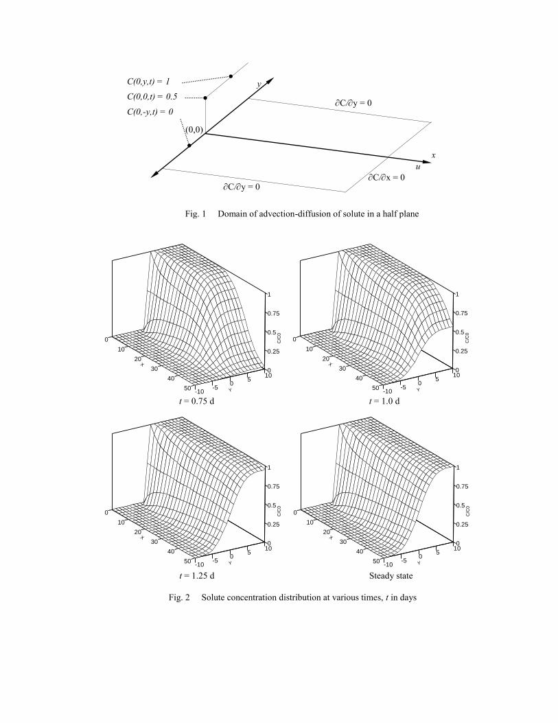
Fig. 1 Domain of advection-diffusion of solute in a half plane

0

0.25

0.5

0.75

1

C/C

0

0

10

20

30

40

50

X

-10-5

05

10

Y

Y

Z

X

Frame 001 11 Jun 2008

0

0.25

0.5

0.75

1

C/C

0

0

10

20

30

40

50

X

-10-5

05

10

Y

Y

Z

X

Frame 001 11 Jun 2008

0

0.25

0.5

0.75

1

C/C

0

0

10

20

30

40

50

X

-10-5

05

10

Y

Y

Z

X

Frame 001 11 Jun 2008

0

0.25

0.5

0.75

1C

/C0

0

10

20

30

40

50

X

-10-5

05

10

Y

Y

Z

X

Frame 001 11 Jun 2008

Fig. 2 Solute concentration distribution at various times, t in days

t = 0.75 d t = 1.0 d

t = 1.25 d Steady state

y

x

u

C/y = 0

C/x = 0 C/y = 0

C(0,y,t) = 1

C(0,0,t) = 0.5

C(0,-y,t) = 0

(0,0)

0

0.2

0.4

0.6

0.8

1

-10 -5 0 5 10y, cm

C/C

0

0

0.2

0.4

0.6

0.8

1

-10 -5 0 5 10y, cm

C/C

0

0

0.2

0.4

0.6

0.8

1

-10 -5 0 5 10y, cm

C/C

0

0

0.2

0.4

0.6

0.8

1

-10 -5 0 5 10y, cm

C/C

0

Fig. 3 Comparison of dimensionless concentration distribution computed using LSGS

method with analytical solution at x = 50 cm. (○ LSGS, analytical [15])

t = 0.75 d t = 1.0 d

t = 1.25 d Steady state

0 1 2 3 4 5 60

0.5

1

Frame 001 05 Mar 2009

Fig. 5 Evolution of the flow over the square obstacle in time: streamlines at (a) t = 1.0, (b) t = 2.0, (c) t = 5.0, (d) steady state and (e) pressure contours at steady state

Fig. 4 Mesh () used for unsteady flow over a square obstacle

Frame 001 05 Mar 2009

Frame 001 05 Mar 2009

Frame 001 05 Mar 2009

-0.035

-0.010-0.000 0.001

0.033

0.144

0.3230.495

0.671

0.798

0.864

Frame 001 05 Mar 2009

-0.010

-0.080-0.2

23

-0.498-0.636

-0.2

230.1

90

0.328

0.407

0.407

-0.395

-0.0

80

-0.3

95

Frame 001 05 Mar 2009

(a)

(b)

(c)

(d)

(e)

Frame 001 16 Jun 2008

Fig. 6 Mesh (4074 bilinear elements) for unsteady flow over rectangular cylinder

Fig. 7 Results for unsteady flow past rectangular cylinder at Re = 150: (a) instantaneous streamlines,

(b) pressure contour, (c) Variation of vertical velocity at x/L 1.5 from trailing edge

Frame 001 18 Jun 2008

Frame 001 18 Jun 2008

St = 0.1322

-0.08

-0.04

0

0.04

0.08

0.12

45 50 55 60 65 70 75 80 85

time, t

ver

tica

l v

elo

city

,v v

nn

(a)

(b)

(c)

St = 0.1577

-0.1

-0.06

-0.02

0.02

0.06

0.1

85 90 95 100 105 110 115

time, t

vert

ical

velo

cit

y,

v .

.

Frame 001 07 Jul 2008

Frame 001 08 Jul 2008

(a)

(b)

(c)

Fig. 8 Results for unsteady flow past rectangular cylinder at Re = 300: (a) instantaneous streamlines,

(b) pressure contour, (c) Variation of vertical velocity at x/L 1.5 from trailing edge