www.elsevier.com/locate/compfluid

Computers & Fluids 35 (2006) 227–240

Optimizing lattice Boltzmann simulations for unsteady flows

A.M. Artoli, A.G. Hoekstra *, P.M.A. Sloot

Section Computational Science, University of Amsterdam, Kruislaa 403, 1098 SJ Amsterdam, The Netherlands

Received 28 November 2003; received in revised form 27 July 2004; accepted 17 December 2004

Available online 21 April 2005

Abstract

We present detailed analysis of a lattice Boltzmann approach to model time-dependent Newtonian flows.

The aim of this study is to find optimized simulation parameters for a desired accuracy with minimal com-

putational time. Simulation parameters for fixed Reynolds and Womersley numbers are studied. We inves-tigate influences from the Mach number and different boundary conditions on the accuracy and

performance of the method and suggest ways to enhance the convergence behavior.

� 2005 Elsevier Ltd. All rights reserved.

PACS: 47.11.+j; 87.19.UV

1. Introduction

For years to come, a necessity for efficient and robust computational fluid dynamics (CFD)solvers will be demanded by scientists working at the edge of available computer power. It hasbeen understood by many authors that transport phenomena can be studied from a kinetic theorypoint of view [1,2] where an alternative description is given through the Boltzmann equation forthe probability density function f ðt;~x;~nÞ for particles of velocity ~n at point ~x and time t. TheBoltzmann equation was mainly developed for ideal gases, but in the limit of small mean free path

0045-7930/$ - see front matter � 2005 Elsevier Ltd. All rights reserved.

doi:10.1016/j.compfluid.2004.12.002

* Corresponding author. Tel.: +20 525 7543; fax: +20 525 7490.

E-mail addresses: artoli@science.uva.nl (A.M. Artoli), alfons@science.uva.nl (A.G. Hoekstra), sloot@science.uva.nl

(P.M.A. Sloot).

URL: http://www.science.uva.nl/research/scs (A.G. Hoekstra).

228 A.M. Artoli et al. / Computers & Fluids 35 (2006) 227–240

between molecular collisions, a gas may be considered as a continuum fluid. The main advantageover the Navier–Stokes equations is the capability of the Boltzmann solution to capture complexfluid behavior such as multicomponent flow and flow in porous media. After the link between theBoltzmann equation and hydrodynamics was well established (see e.g. Ref. [3]), the need for effi-cient numerical solvers was large, since the Boltzmann equation is hard to solve in general. Per-turbation methods such as the Chapmann–Enskog and Hilbert techniques are common numericalapproaches taken. After simplifying the collision operator, solutions are obtained as asymptotesto the Boltzmann equation. However, these solutions are not readily applicable to flows of com-mon engineering interest.A new way of solving the Boltzmann equation has been realized soon after Frisch et al. [4]

introduced the lattice gas cellular automata (LGCA), an automata that is capable of capturingcomplex fluid nature by obeying local conservation laws. A few shortcomings of the LGCA wererecognized and intensively investigated. Those are, among others, the lack of Galilean invariance,statistical noise, low Reynolds number (high viscosity) and exponential complexity of the collisionoperator [5–7]. The lattice Boltzmann method was introduced to remove these shortcomings [8].The idea is simply to replace the Boolean LGCA occupation numbers ni with ensemble-averagedpopulations fi = <ni>. The system has become capable to capture many features in the evolvingnature [9–11]. A little later, the lattice Boltzmann equation has been realized as a direct discreti-zation of the simplified Boltzmann equation [12], independent of lattice-gas automata, as will bedemonstrated subsequently.

2. The lattice Boltzmann equation

We start from the Boltzmann equation with the BGK approximation for the collision operator

dfdt

þ~n � rf ¼ � 1

kðf � gÞ ð1Þ

which describes the time evolution of the probability distribution function f � f ð~x;~n; tÞ of a singleparticle moving with a microscopic velocity~n and relaxing with a collision relaxation time k to aMaxwellian equilibrium distribution

g ¼ q

ð2pRT Þ32

exp �ð~n �~uÞ2

2RT

!ð2Þ

which is a function of the ideal gas constant R, the macroscopic quantities q, ~u and T, and themicroscopic velocity~n, with q the density,~u the fluid velocity and T its temperature. The macro-scopic quantities are computed from the microscopic moments of f. Approximating the formalintegral of the Boltzmann equation over a time step dt and ignoring the leading terms of O(dt

2)by the use of Taylor expansion, yields a first order in time discretization for the Boltzmann equa-tion [12] given by

f ð~xþ~ndt; t þ dtÞ � f ð~x; tÞ ¼ � 1

s½f ð~x; tÞ � gð~x; tÞ ð3Þ

where s ¼ kdtis the dimensionless relaxation time.

A.M. Artoli et al. / Computers & Fluids 35 (2006) 227–240 229

Discretization of velocity is needed to approximate the hydrodynamic moments and thereaftercompute the equilibrium distribution. A lattice structure that satisfies conservation laws and guar-antees the symmetry needed by the Navier–Stokes solutions is obtained. Different lattice struc-tures can be used [12], such as the three dimensional Cartesian grid with 19 discrete velocities(referred to as D3Q19) used in this paper. D3Q19 has 6 particles moving in the principal direc-tions with a constant speed v = dx/dt, 12 particles moving along the diagonals with a speed

ffiffiffi2

pv

and a rest particle in the center of a cube. The equilibrium distribution function is approxi-mated to f eq

i by a truncated velocity expansion up to a desired accuracy (usually to the secondorder in u2)

g � f eqi ¼ qwi 1þ 3

v2~ei �~uþ

9

2v4ð~ei �~uÞ2 �

3

2v2~u �~u

� �ð4Þ

where ~ei is the velocity of the particle along the direction i, with i = 0,1,2, . . . ,z, where z is thenumber of particle distributions of the model (z = 19 for D3Q19) and wi a weight coefficient.The hydrodynamic density q and the macroscopic velocity ~u are determined in terms of the par-ticle distribution functions from

q ¼Xi

fi ¼Xi

f ðeqÞi ð5Þ

and

q~u ¼Xi

~eifi ¼Xi

~eifðeqÞi ð6Þ

Eq. (3) then becomes

fið~xþ~edt; t þ dtÞ � fið~x; tÞ ¼ � 1

s½fið~x; tÞ � f ðeqÞ

i ð~x; tÞ ð7Þ

which is usually known as the lattice Boltzmann BKG equation (LBGK).It can be shown that the LBGK is equivalent to a second order discretization of the Navier–

Stokes equations [12] if the viscosity is defined by

m ¼ Cv2dt s � 1

2

� �ð8Þ

and the pressure as

p ¼ qc2s ð9Þ

where C is a lattice-dependent coefficient, equal to 1/3 for D3Q19, and

cs ¼ vffiffiffiffiC

pð10Þ

is the ‘‘pseudo’’ speed of sound in the system, which is also lattice dependent. We can also provethat the a component of the symmetric stress tensor on a surface perpendicular to b-axis is givenby [11,13]

230 A.M. Artoli et al. / Computers & Fluids 35 (2006) 227–240

rab ¼ �qc2sdab � 1� 1

2s

� �Xzi¼0

f ð1Þi eiaeib ð11Þ

where f ð1Þi is the non-equilibrium part of the distribution function and dab is the unit tensor. Here,

we emphasize that the quantity f ð1Þi eiaeib is usually computed during the collision process. There-

fore, the stress tensor components can be obtained independent from the velocity fields. Thisstrongly enforces the lattice Boltzmann method when compared to other CFD methods whichall estimate the stress tensor components from the simulated velocity field. It should be noted thatthe stress tensor components can be computed with the lattice Boltzmann equation with secondorder accuracy. The benefit over other CFD techniques in computing the stress tensor is clearwhen dealing with flow in complex geometry of irregular cross-sections or flows characterizedby large velocity gradients. The lattice Boltzmann equation can model macroscopic fluid flowswith second order accuracy in both space and time [e.g. 14,15]. However, this accuracy is com-monly degraded by four major sources. These are the boundary conditions, the compressibilityerror, the discretization error and the momentum error. In this study, we investigate the accuracyand performance of the lattice Boltzmann method for unsteady flow simulations.The aim of this study is to optimize the method for best accuracy within a minimum possible

computational time. Different ways to refine the computational lattice are studied and their influ-ences on both accuracy and convergence are investigated. The study concentrates on the influenceof the Mach number and boundary conditions on the accuracy and performance. We will firstpresent and discuss results of unsteady flow simulations in a rigid tube, investigate effects fromdifferent lattice refinement techniques on the accuracy and performance of the method and suggestways to enhance the performance.

3. Simulations

We have conducted a number of different simulation studies for unsteady flow in a 3D tube.First, we simulate systolic flow in a tube and validate the results against the analytical Womersleysolutions. We then compare the bounce-back rule (BBL) with the body-fitted Bouzidi boundaryconditions with first (BBC1) and second (BBC2) order interpolations at different Mach numbers.Finally, different ways of reducing the errors by grid refinement techniques are presented andinvestigated under their accuracy and convergence behavior.

3.1. Systolic flow in a straight rigid tube

We compute time-dependent flow in a 3D tube. In all simulations, the pressure gradient in thetube is computed from a measured systolic pressure at the entrance of the human abdominalaorta, using Fourier transformations, up to the 8th harmonic. Simulation parameters are set to ob-tain a maximum Reynolds number Re ¼ UD

m ¼ 590 and a Womersley parameter a ¼ Rffiffiffixm

p¼ 16,

where R = D/2 is the radius of the tube, x = 2p/T is the angular frequency and T = 1/f is the per-iod, with f the frequency. Pressure boundary conditions are used for the inlet and the outlet [11]boundaries and, for the walls, either the bounce back on the links (BBL) or the Bouzidi [16]boundary conditions with first (BBC1) and second order (BBC2) interpolations are used.

A.M. Artoli et al. / Computers & Fluids 35 (2006) 227–240 231

Obtained velocity profiles over a complete period are compared to the analytical Womersleysolutions [24]

Fig. 1

Mach

uðy; tÞ ¼X8m¼1

� Am

qmxe�imxt 1�

J 0ffiffiffiffiffiffimb

py

� J 0

ffiffiffiffiffiffimb

pR

� !" #

ð12Þ

where J0 is the zeroth order Bessel function of the first type, Am is the amplitude of pressure gra-dient and b = �ix/m = �im(a/R)2 for the mth Fourier harmonic. The obtained shear stress is com-pared to the one derived from the above equation.The computational mesh is a simple Cartesian lattice. The diameter of the tube is represented

by D lattice nodes. The length of the tube is always taken to be 3 · D. We start by setting D = 74lattice nodes. First, BBL is used to simulate systolic flow in the tube. The simulation parametersare set to yield the required Womersley and Reynolds numbers which are kept fixed. For this sim-ulation, T = 2000, and s = 0.55, giving a = 16 and Re = 590. Fig. 1(a) shows a density plot ofobtained velocity profiles over the whole period. The corresponding shear stress values arecontoured in Fig. 1(b). From this figure we observe that the velocity has high gradients very closeto the walls (in the region 3R/4 < y < R) and gets flat toward the center of the tube. The shearstress vanishes in the center and is high and oscillating near to the walls.Samples of obtained velocity profiles at different times of the systolic cycle are shown in Fig. 2

compared to the real part of the analytical Womersley solutions. As clearly shown in this figure,the agreement with the analytical solution is quite good. We define the relative error in velocity ateach time-step as

Eu ¼Pn

i¼0juthðxiÞ � ulbðxiÞjPni¼1juthðxiÞj

ð13Þ

where uth(xi) is the analytical solution for the axial velocity and ulb(xi) is the velocity obtainedfrom the LBE simulations. The overall relative error is averaged over the period and will be

. Contour density plots of obtained (a) velocity and (b) shear stress during a full systolic cycle with T = 2000,

= 0.05, Re = 590 and a = 16. Dark areas stands for high values of velocity and shear stress in lattice units.

Fig. 2. Samples of obtained velocity profiles (dots) in lattice units during the systolic cycle in a 3D tube, compared to

the analytical Womersley solutions (lines), using the bounce-back rule at Mach = 0.05, Re = 590 and a = 16. The time

during systole for the curves are from 0 to 56T with steps of 1

6T .

232 A.M. Artoli et al. / Computers & Fluids 35 (2006) 227–240

referred to as the average error. The bounce back on the links yields an average error of 0.12 at aMach number of 0.05 for this specific simulation. This indicates that, even with the bounce-backrule, acceptable accuracy can be obtained for ‘‘engineering applications’’.Using the same simulation parameters, we have conducted another set of simulations after

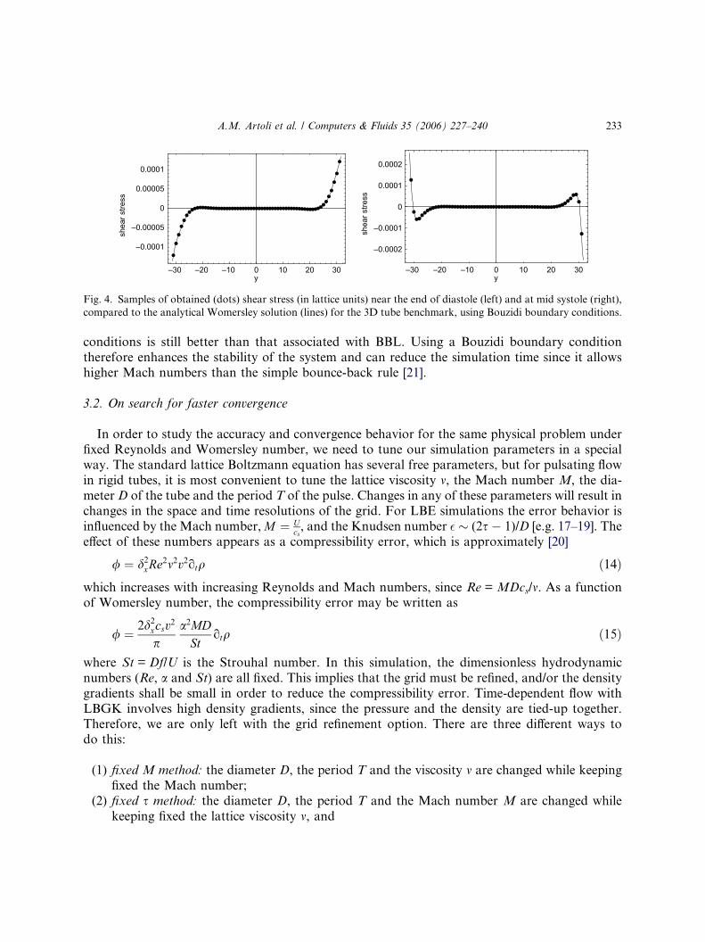
replacing the bounce back on the links with Bouzidi boundary conditions. The agreement withanalytical solutions enhances significantly, as shown in Fig. 3. The average error reduces toapproximately 0.03. As shown in Fig. 4, similar agreement is achieved for the shear stress. It isto be noted that the Bouzidi boundary condition does not perform better than the bounce backat points with large velocity gradients, as it uses interpolation.We also note that it is possible to go for higher Mach numbers with Bouzidi boundary condi-

tions while still having better accuracy than those with BBL at a considerably lower Mach num-ber. Even with a 10 times higher Mach number, the error associated with the Bouzidi boundary

Fig. 3. Samples of obtained velocity profiles (dots) in lattice units during the systolic cycle in a 3D tube, compared to

the analytical Womersley solutions (lines) using Bouzidi boundary conditions at Mach = 0.05, Re = 590 and a = 16. The

time during systole for the curves are from 0 to 56T with steps of 1

6T .

—30 —20 —10 0 10 20 30y

—0.0001

—0.00005

0

0.00005

0.0001

shea

r stre

ss

—30 —20 —10 0 10 20 30y

—0.0002

—0.0001

0

0.0001

0.0002

shea

r stre

ss

Fig. 4. Samples of obtained (dots) shear stress (in lattice units) near the end of diastole (left) and at mid systole (right),

compared to the analytical Womersley solution (lines) for the 3D tube benchmark, using Bouzidi boundary conditions.

A.M. Artoli et al. / Computers & Fluids 35 (2006) 227–240 233

conditions is still better than that associated with BBL. Using a Bouzidi boundary conditiontherefore enhances the stability of the system and can reduce the simulation time since it allowshigher Mach numbers than the simple bounce-back rule [21].

3.2. On search for faster convergence

In order to study the accuracy and convergence behavior for the same physical problem underfixed Reynolds and Womersley number, we need to tune our simulation parameters in a specialway. The standard lattice Boltzmann equation has several free parameters, but for pulsating flowin rigid tubes, it is most convenient to tune the lattice viscosity m, the Mach number M, the dia-meter D of the tube and the period T of the pulse. Changes in any of these parameters will result inchanges in the space and time resolutions of the grid. For LBE simulations the error behavior isinfluenced by the Mach number,M ¼ U

cs, and the Knudsen number � � (2s � 1)/D [e.g. 17–19]. The

effect of these numbers appears as a compressibility error, which is approximately [20]

/ ¼ d2xRe2m2v2otq ð14Þ

which increases with increasing Reynolds and Mach numbers, since Re =MDcs/m. As a functionof Womersley number, the compressibility error may be written as

/ ¼ 2d2xcsv2

pa2MDSt

otq ð15Þ

where St = Df/U is the Strouhal number. In this simulation, the dimensionless hydrodynamicnumbers (Re, a and St) are all fixed. This implies that the grid must be refined, and/or the densitygradients shall be small in order to reduce the compressibility error. Time-dependent flow withLBGK involves high density gradients, since the pressure and the density are tied-up together.Therefore, we are only left with the grid refinement option. There are three different ways todo this:

(1) fixed M method: the diameter D, the period T and the viscosity m are changed while keepingfixed the Mach number;

(2) fixed s method: the diameter D, the period T and the Mach number M are changed whilekeeping fixed the lattice viscosity m, and

234 A.M. Artoli et al. / Computers & Fluids 35 (2006) 227–240

(3) fixed D method: the viscosity m, the period T and the Mach number M are all changed whilekeeping fixed the diameter D.

The effects of these changes on the grid resolution are shown in Table 1, in which we assume afactor of n change in one of the parameters and compute the corresponding changes in the otherparameters in order to keep fixed Reynolds and Womersley numbers. From this table, we can pre-dict the computational efficiency of each approach. For instance, the fixedM approach involves ntimes decrement in dx (which increases the number of grid points n3 times) and n times reductionin dt which scales the total simulation time by n4 per systolic cycle. The fixed s method scales thesimulation time per cycle as n5 and the fixed D method scales it as n. Although it is easy to see thatthe last method is faster while the second one is more accurate, a combination of accuracy andperformance is not trivial. The fixed M method does not involve reduction of the Mach number,which is a major contribution to accuracy enhancement when considering time-dependent flowsand, therefore, it is not attractive in this study. Accordingly, we have performed 2 sets of simula-tions corresponding to the fixed s and the fixed D methods. They are discussed below.

3.2.1. Accuracy and performance with the fixed D method

We have selected three sets of parameters to study the error behavior produced by this tech-nique. First, we have performed a reference simulation at M = 0.5, D = 74, s = 1, T = 200, andwe took the magnitude of the pressure gradient as G = 0.0011. This pressure gradient will resultin the wanted Mach number. Then, two other parameter sets are selected with the aid of Table 1.The pressure gradient must be reduced by a factor n2 to give the correct Mach number scaling.The errors associated with each boundary condition at three different Mach numbers are shownin Table 2, in which n = 1 represents the reference simulation. In all simulations, the system is ini-tialized from rest and the simulation ends after 40 complete systolic cycles. The simulations wereperformed on 8 nodes of a Beowulf cluster using slice decomposition. The mean time per iterationis about 0.45 s using the bounce back and 0.47 using the Bouzidi boundary conditions on 8 pro-cessors. The total execution time for 40 complete cycles is therefore 18T for the bounce back and18.8T for the Bouzidi boundary conditions. For low Mach numbers, this difference in executiontime scales as hours (4.5 h for n = 100).From this table we notice that for BBC1 with M = 0.5, the agreement with the analytical solu-

tions is still better than that for a 10 times smaller Mach number with BBL.It is also apparent that Bouzidi boundary conditions are more stable than the bounce-back rule

at high Mach numbers, but the situation reverses for lower Mach numbers.

Table 1

Relative changes in simulation parameters under fixed Reynolds and Womersley numbers with respect to a factor of n

change in one of the parameters of a reference simulation

Lattice parameter D 0/D m0/m T 0/T U 0/U d0x=dx d0t=dt M 0/M

Fixed D 1 1/n n 1/n 1 1/n 1/n

Fixed s n 1 n2 1/n 1/n 1/n2 1/n

Fixed M n n n 1 1/n 1/n 1

The prime refers to the new simulation.

Table 2

Average error for unsteady flow in a tube with D = 74 using BBL, BBC1 and BBC2 boundary conditions at three

different Mach numbers

n

1 10 100

Eav, BBL Not stable 0.120 0.027

Eav, BBC1 0.0627 0.0352 0.0253

Eav, BBC2 0.0615 0.0102 Not stable

A.M. Artoli et al. / Computers & Fluids 35 (2006) 227–240 235

In addition, we have noticed that BBC1, which interpolates data up to the first fluid node ismore stable than the second order interpolation scheme (BBC2) which interpolates data usingtwo neighboring fluid nodes. This may be attributed to effects from interpolation in a region oflarge velocity gradients in the case of BBC2.From this set of simulations, we conclude that it would be faster, more stable and more accu-

rate to use a Bouzidi boundary condition than the simple bounce back.

3.2.2. Accuracy and performance with the fixed s method

Given the n5 scaling of computing time per systole (see Table 1), the fixed s method is most pre-ferably studied by first trying to reduce the computing time as much as possible, and then observ-ing the associated errors. These errors can then be compared to those in the fixed D method, afterwhich one can decide which scaling method to use. In order to reduce the simulation time, it isnecessary to have a large time-step in a coarse grid at a high Mach number. To attain that, weuse the fixed s method to perform a set of simulations in which the period is set to minimum pos-sible value that leads to a stable solution on the coarsest grid. Then the corresponding values forthe pressure gradient and the relaxation parameter are set to yield the desired Womersley andReynolds numbers. The convergence behavior is studied by grid refinement in both dx and dt,as explained in Table 1. The obtained average errors associated with the three used boundary con-ditions are plotted in Fig. 5. We notice that the accuracy of the bounce-back rule approaches thatof the Bouzidi boundary conditions as the grid is refined. As this method results in reducing dx, dtand the pressure gradient, both accuracy and performance are significantly enhanced, since allparameters influencing the error are under control. Moreover, with this method, solutions withperiods smaller than the fixed D method are stable and therefore the simulation time is less,but it scales as n5.The convergence behavior as a function of time for this method is shown in Fig. 6, which shows

the absolute error (difference between the analytical and obtained velocity profiles) at differentsimulation times. From this figure, we observe that the method converges to a reasonable accu-racy after 40 complete periods, similar to the fixed D method, but with a major computationalgain, since dt is larger. This figure also illustrates that the error localizes near to the walls, wherelarge gradients exist, and the accuracy does not enhance noticeably near to the walls on the samegrid. The accuracy close to the wall may be enhanced by considering local grid refinement or run-ning the simulation at lower Mach numbers. Table 3 lists the error dependence as a function ofsimulation time for BBL, BBC1 and BBC2 boundary conditions for a tube with D = 65 latticenodes. The error is reasonably comparable to that obtained by using the fixed D method. The

0.01

0.1

1

10 100

Ave

rage

Err

or

N

BBLBBC

BBC2

Fig. 5. Convergence behavior obtained by reducing the grid spacing n times, time-step n2 times and increasing the

period n2 times, for the BBL, BBC and BBC2 boundary conditions as a function of grid points representing the

diameter of the tube. The relaxation parameter is kept constant and the body force is reduced n3 times to return

the same Reynolds and Womersley parameters at Re = 590 and a = 16.

—30 —20 —10 0 10 20 30y

0

0.005

0.01

0.015

0.02

Ev

Fig. 6. Absolute error (Ev), dE, computed for the velocity field at t = 20T (top curve), 30T, 40T and 50T (bottom

curve). The diameter of the tube is represented by 65 nodes and the period is T = 360 sampling points. The average

errors are tabulated in Table 3. The bounce back on the links shows similar behavior with larger spread (see text).

Table 3

Temporal relative error, Eu(T) for BBL and BBC1 and BBC2 boundary conditions with D = 65 lattice nodes, T = 360,

Re = 590 and a = 16

Time

0 10T 20T 30T 40T 50T

Eu(T), BBL 0.9950 0.2520 0.0698 0.0279 0.0200 0.0200

Eu(T), BBC1 0.9950 0.2769 0.0615 0.0280 0.0200 0.0197

Eu(T), BBC2 0.9950 0.2747 0.2520 0.0866 0.0350 0.0560

236 A.M. Artoli et al. / Computers & Fluids 35 (2006) 227–240

mean deviation of the error is 0.02 for the bounce back on the links and two times larger for theBouzidi boundary conditions.

A.M. Artoli et al. / Computers & Fluids 35 (2006) 227–240 237

In conclusion, this method is computationally more feasible than the fixed D method. It is rec-ommended to use it while keeping D and T to their minimum values that returns stable solutions.

3.3. Performance analysis

Convergence of the lattice Boltzmann method to steady state is significantly affected by twolocal processes: initialization and boundary conditions. In this section, we focus on the influenceof these processes on the convergence behavior.

3.3.1. Performance and walls boundary conditionsAs mentioned before, boundary conditions need to be defined at walls, inlets and outlets. For

the walls, two categories of boundary conditions can be recognized; bounce backs and Bouzidiboundaries. The bounce-back rule is a very efficient boundary condition since it only involves asingle memory swapping process for each relevant distribution on each node on the surface ofthe simulated object. For Bouzidi boundaries, the exact position of the walls is determined at leastonce if the boundary is fixed and need to be computed dynamically for moving boundaries. This isby itself more costly than using the bounce-back rule. In addition, using Bouzidi boundary con-ditions involves first or second order interpolation or extrapolation for velocity, distribution func-tions or density or a combination of some or all of them. As demonstrated earlier in this article,use of a Bouzidi boundary condition enhances the accuracy but is computationally more intensivecompared to the simple bounce back at the same Mach number. To gain the accuracy of a Bouzidiboundary condition and a performance similar to the bounce back, an accelerating technique maybe applied. The Mach number annealing technique has been recently introduced by the authors[21] to accelerate unsteady flow simulations. This annealing process is based on using thebounce-back rule to start the simulation at relatively high Mach number and wait until the systemconverges, then reduce the Mach number to a lower value M 0 to obtain a desired accuracy. Thesystem directly adapts to the new parameters defining the new Mach number. We have performeda number of simulations using this annealing technique. The gain in computational time can bedetermined as follows. We assume that after simulating 40 full systoles, the simulation has con-verged (see e.g. Fig. 6 and Table 3). We have also observed this in simulations of real arteries (datanot shown). We therefore perform our simulations by first running 40 systoles, and then simulateone final systole in which we measure the wanted observables (velocity fields, shear stress tensor).To obtain the same Reynolds and Womersley numbers, the period and the kinematic viscositymust be modified. Calling T0 the period on the high Mach number and Tn the period on small,annealed Mach number we write Tn = mT0 and mn = m0/m. The gain in computational time ob-tained by Mach number annealing then is

Gain ¼ 41m40þ m

ð16Þ

where m =M/M 0 is the annealing factor. For details, we refer to Ref. [21].

3.3.2. Inlet and outlet conditionsFor LBE simulations, a number of inlet and outlet conditions are available. The most com-

monly used are periodic boundary conditions, in which distributions leaving the simulation box

238 A.M. Artoli et al. / Computers & Fluids 35 (2006) 227–240

at the outlet are re-injected at the inlets and vice-versa. Periodic boundary conditions involve onlymemory swapping operations. Although they are fast, and accurate, they can only be used forperiodic geometry. For non-periodic geometry, inlets and outlets need to be treated differentlyin the following manner:

• Velocity and pressure: assign one and compute the other [22], assign both (only for inlets),extrapolate or assume no flux normal to the walls (only for outlets).

• Unknown distributions: compute explicitly [22], set to their equilibrium, copy from nearestneighbors, interpolate or extrapolate.

For the first item, if the velocity or the pressure are computed one from the other, at least 15additions and two multiplications are needed per node on the boundary and therefore is atleast 15 times more expensive than periodic boundary conditions. Extrapolation and no-fluxschemes are far better in terms of accuracy and performance than computing velocity or pres-sure from one another, but they are only suitable for the outlets. A reasonable choice for time-dependent flow in irregular geometry is then to assign pressure and compute velocity at theinlet, no-flux at the outlets and set the unknown distributions to their equilibrium values. Ifthe outlets are far enough from inflow, copying from upstream would be the most efficient out-let condition.

3.3.3. Initial conditionsTime-dependent flow involves large density fluctuations. Although it increases compressibility

errors, this reduces the initialization influence on convergence behavior. However, the way inwhich the simulation box is initialized has little effect on the final flow fields [23]. Since the Boltz-mann equation assumes that the system is not far from equilibrium, a correct and reasonable ini-tialization technique is to compute the equilibrium distributions from expected macroscopicparameters and set each distribution to its equilibrium with a small perturbation, We haveadopted this initialization process in all our simulations. It is noted that more sophisticated ini-tialization techniques such as second order interpolations from the boundaries may be usefulbut they complicate the standard LBE scheme.

4. Conclusions

An aortic pressure is used as an inlet condition to drive the flow in a 3D rigid tube and theWomersley solution is recovered to an acceptable accuracy. Different ways to change the spatialresolution in the simulations where studied, and the resulting errors and convergence behaviorwere discussed. The influence of walls, inlet and outlet boundary conditions on accuracy and per-formance is studied in detail. We have shown that the lattice Boltzmann BGK method is an accu-rate and efficient method as a solver for time-dependent flows. Different methods for performingtime-dependent flows at fixed simulation parameters are tested in terms of accuracy and perfor-mance. We have demonstrated three different grid-refinement scenarios for error analysis of un-steady flow simulations: fixed spatial resolution (the fixed D method), fixed lattice viscosity (the

A.M. Artoli et al. / Computers & Fluids 35 (2006) 227–240 239

fixed s method) and fixed Mach number (the fixed M method). Our study allows users of theLBGK method to find optimal simulation parameters for their specific (time periodic) flowproblem.We have shown that it would be more accurate and relatively stable to use Bouzidi boundary

conditions at high Mach numbers, or still use the bounce back on the links at lower Mach num-bers. It is to be noted that the Bouzidi boundary conditions become very expensive when used formoving boundaries, since the wall–fluid distance has to be computed at each time step. However,the cost of the bounce-back rule for moving boundaries is the same for that for static ones. Weclaim that the bounce back on the links could be more efficient than the Bouzidi boundary con-ditions if used at low Mach numbers when the Mach number annealing technique is used. SinceBouzid boundary conditions are complex and computationally intensive for unstructured and dy-namic geometry, the bounce back on the link with Mach number annealing is a promising tech-nique for studying such kind of applications.

Acknowledgement

This work is partially funded by the Steunfonds Soedanese Studenten, Leiden, TheNetherlands.

References

[1] Caflisch RE. Fluid dynamics and the Boltzmann equation. In: Lebowitz JL, Montroll EW, editors. Non-

equilibrium phenomena I: The Boltzmann equation. North-Holland Publishing Company; 1983. p. 195–

226.

[2] Ramaswamy S. Adv Phys 2001;50:297.

[3] Cercingnani C. J Quant Spec Rad Trans 1971;197:973.

[4] Frisch U, Hasslacher B, Pomeau Y. Phys Rev Lett 1986;56:1505.

[5] Higuera FJ, Succi S, Benzi R. Europhys Lett 1989;9:345.

[6] Rothmann DH, Zaleski S. Lattice-gas cellular automata, simple models of complex hydrodynamics. Cam-

bridge: Cambridge University Press; 1997.

[7] Rivet JP, Boon JP. Lattice gas hydrodynamics. Cambridge, UK: Cambridge University Press; 2001.

[8] McNamara GR, Zanetti G. Phys Rev Lett 1988;61:2332.

[9] Chen S, Doolen GD. Ann Rev Fluid Mech 1998;30:329.

[10] Succi S. The lattice Boltzmann equation for fluid dynamics and beyond. Oxford, UK: Oxford University Press;

2001.

[11] Artoli AM, Hoekstra AG, Sloot PMA. Int J Mod Phys C 2002;13:1119.

[12] He X, Luo LS. Phys Rev E 1997;56:6811.

[13] Hou S, Zou Q, Chen S, Doolen G, Cogley AC. J Comput Phys 1995;118:329.

[14] Filippova O, Hanel D. Int J Mod Phys C 1998;9:1271.

[15] Mei RW, Luo LS, Shyy W. J Comput Phys 1999;155:307.

[16] Bouzidi M, Firdaouss M, Lallemand P. Phys Fluids 2001;13:3452.

[17] Zou Q, Hou S, Chen S, Doolen GD. J Stat Phys 1995;81:35.

[18] He XY, Luo LS. J Stat Phys 1997;88:927.

[19] Guo ZL, Shi BC, Wang NC. J Comput Phys 2000;165:288.

240 A.M. Artoli et al. / Computers & Fluids 35 (2006) 227–240

[20] Holdych DJ, Noble DR, Georgiadis JG, Buckius RO. J Comput Phys 2004;193:595.

[21] Artoli AM, Hoekstra AG, Sloot PMA. Int J Mod Phys C 2003;14:835.

[22] Zou Q, He X. Phys Fluids 1997;9:1591.

[23] Skordos PA. Phys Rev E 1993;48:4823.

[24] Womersley JR. J Physiol 1955;127:553.