Stabilization of thermal lattice Boltzmann models

Journal of Statistical Physics, Vol. 81. Nos. 1/2, 1995

Stabilization of Thermal Lattice Boltzmann Models

Guy R. McNamara, l Alejandro L. Garcia, 2"3 and Berni J. Alder 2

Received December 13, 1994;final May 16, 1995

A three-dimensional thermal lattice-Boltzmann model with two relaxation times to separately control viscosity and thermal diffusion is developed. Numerical stability of the model is significantly improved using Lax-Wendroff advection to provide an adjustable time step. Good agreement with a conventional finite- difference Navier-Stokes solver is obtained in modeling compressible Rayleigh- B6nard convection when boundary conditions are treated similarly.

KEY WORDS: Lattice-Boltzmann equation; hydrodynamics; boundary conditions; compressible convection.

1. I N T R O D U C T I O N

The lattice gas au tomaton (LGA) method 11"2) models fluid dynamic behavior by creating a fictitious molecular dynamical world of particles moving on a regular lattice. These particles travel between neighboring lattice sites, arriving synchronously at the lattice sites at integral multiples of the simulation time step, where they engage in collisions that conserve particle number , momentum, and (for thermal models 13'41) energy. The LGA models are Boolean systems that allow only zero or one particle at each site for each of the permitted particle velocities. Macroscopic quantities, such as mass density and fluid velocity, are obtained by spatial or temporal averaging to eliminate the large amoun t of statistical noise in the LGA calculations.

Theoretical Divisiort and Center for Non-Linear Studies, Los Alamos National Laboratory, Los Alamos, New Mexico 87545.

-'Institute for Scientific Computing Research L-416, Lawrence Livermore National Laboratory, Livenr~ore, California 94550.

3 Permanent address: Department of Physics, San Jose State University, San Jose, California 95192-0106.

395

0022-4715/95/1000-0395507.50/0 �9 1995 Plenum Publishing Corporation

396 McNamara et al.

The lattice Boltzmann equation (LBE) model eliminates this statistical noise by directly simulating the ensemble-averaged behavior of an LGA system. The LGA's Boolean variables are replaced by floating point variables f~(r) representing the expected number of particles traveling in the c~th direction at position r of the lattice. The collision phase of the LGA is replaced by an LBE collision operator that redistributes the incoming particle mass among the outgoing particle velocities in such a way as to relax toward a local equilibrium distribution determined from the local conserved densities.

The earliest LBE models ~5~ were direct transcriptions of existing LGA models with the LBE equilibrium distribution and collision operator dictated by the collision rules of the LGA model. As such, these systems carried with them the defects of the original LGA model, such as the lack of Galilean invariance and velocity-dependent pressure. Later LBE implementations ~6"7~ depart from the constraints of preexisting LGA models so that the Fermi-Dirac equilibrium distribution arising from the Boolean nature of an LGA is replaced by a more general equilibrium distribution that eliminates the Galilean invariance and pressure defects as well. Furthermore, to simplify the analysis, the nonlinear collision process of the LGA can be replaced by linear relaxation to equilibrium. In this generalization, however, the particle nature of the LGA method, and the numerical stability connected with it, have been lost. Initially, LBE models included only mass and momentum as conserved quantities; these models were found to be remarkably stable.

In some cases, the similarity between the Navier-Stokes velocity and temperature equations can be exploited to formulate LBE models that treat temperature as an additional velocity component. For example, simulations of Rayleigh-B6nard convection using a single-speed LBE model of the Boussinesq equations have been performed by Benzi and co-workers, tS~ More recent work, ~9'1~ using multispeed LBE models, has included energy conservation to allow thermal systems to be studied, but no very stable three-dimensional, multispeed LBE model has been found up to now. This article addresses the problem of how to stabilize such models and whether the LBE numerical approach, in general, presents any obvious advantage over conventional techniques in computational fluid dynamics.

2. THE THERMAL LATTICE-BOLTZMANN MODEL

2.1. The Equilibrium Distribution and Collision Operator

Construction of an LBE model requires the specification of the structure of the lattice and the set of permitted particle velocities {c~}, the

Stabilization of Thermal Lattice Boltzmann Models 397

collision operator g-2~p, and the local equilibrium mass distribution f~0).4

The most general restrictions on the form of fro) required to obtain Navier-Stokes behavior require that its lowest 26 moments match those of the Maxwell-Boltzmann distribution, t'l) It so happens that the velocity set consisting of speed-x/~, speed-x/~, and speed-2 particles on a cubic lattice contains 26 elements, and the symmetries of this set match those of the 26 Maxwell-Boltzmann moments. Moreover, all of these moments may be independently specified and thus this velocity set constitutes a minimal LBE model yielding correct Navier-Stokes hydrodynamic behavior with the equilibrium mass distribution ftol uniquely determined. Unfortunately, this model was found to be numerically unstable unless its transport coefficients were made quite large. It should be possible to achieve numerical stability by augmenting the velocity set and making good use of the additional degrees of freedom provided by a larger velocity set, but our attempts in this direction have been unsuccessful. Possible stabilization of the 26-velocity model through an adjustable time step, ti la Lax-Wendroff (see Section 2.3), is currently under study.

An alternative approach to improving stability is to decrease the velocity set. Such a model will necessarily violate some of the velocity moment constraints, and thus will deviate from Navier-Stokes behavior. With care, these deviations can be made to be of sufficiently high order in the velocity u that the resulting model may still be useful for simulating low-Mach-number flows. The model described in the present work uses a three-dimensional cubic lattice with 21 particle velocities: a single popula- tion of stopped particles, six unit velocities connecting lattice sites to nearest neighbors, eight speed-x/~ velocities connecting lattice sites to neighbors across the body diagonal of the unit cell, and six speed-2 velocities directed along the axes of the lattice.

The collision operator and the equilibrium mass distribution are best described in terms of velocity moments of the mass distribution. The postcollisional mass distribution f'~, is generated from the precollisional distribution f , through the collision operator,

f=( , t ) = f ~ ( r , t ) + y ' t ' 2 ctneq~tr t) #

4 The following conventions are used in describing an LBE model: the simulation time step r is taken as the unit of time, the nearest neighbor spacing of the lattice becomes the unit of length, and the model's particles are taken to have unit mass, m = 1. A temperature scale is established by taking the Boltzmann factor k to be unity. Greek indices are used to iterate over the directions of particle motion, Latin subscripts to denote the Cartesian components of vectors and tensors.

822/81/I-2-26

398

Table I.

M c N a m a r a et al.

Veloci ty M o m e n t s of the Equi l ibr ium Mass Dist r ibut ion rio~ Used in the 21-Ve loc i ty Mode l ~

(I) E~f~ ~ p (2) E ~ c ~ f ~ ) pua (3) E~,c] f~ ~ pu2 + 2pc (4) Y.~ (c,~c~ -- ],']o~,,b)f~) pu,,ub -- ~pu'-5,,h

C2{ (OI (5) ~ , ~,,f~ (uz+~e)pu,, (6) ~,, [ c,.,,c:#,c=,.-- ~c](c,,,,6,,,. + c~a,a,,,. + c:,.a,a,} ] fc= m 0 (7) E, c2~(c=,,c~ - �89 ~ 3pu,,uh-puEa,a,

C4 (0)

(9) L [ " ~ - .2 .2_ -, -, .2 -, (o) 5(c ~_,.~ ~,, + c~_,c~ + %>.c J ] f= 0

~p is the mass density, uu is the fluid velocity, and t is the internal energy per unit mass.

where f~nCql = f ~ -.,af(~ The collision opera tor is fully defined by specifying its effect on a complete set of velocity moments ; our model has 21 particle velocities and thus 21 independent moments are required for a complete specification. The five lowest velocity moment s are just the conserved densities [Table I, entries (1)-(3)] . The conserved densities are contained entirely in the equilibrium distribution, and thus the action of the collision opera tor on these moments is irrelevant. Higher moments are associated with viscous and thermal t ransport propert ies [entries (4) and (5) in Table I l: in particular the action of the collision opera tor on the nonequilibrium part of the trace-free second moments determines the viscosity of the model. Similarly, relaxation of the traceful nonequil ibrium third moments controls the thermal conductivity. These viscous and thermal t ransport moments are taken to be eigenvectors of the collision operator , i.e.,

Y', (c=,,c=b - c~,~,,b/3) j',=(,r = (;,s + 1) ~ ( c ~ , c ~ - - ,..aUabl-,;~2"g 12, d=l'(neq )

Z 2 , ( n e q ) - ~ C2f. f(ncq) c=c~, , f , , - (2,. + 1) ~ _=_=,_= t~ ct

where 2.,. and 2c are eigenvalues of t-2. The kinematic viscosity v and the thermal diffusivity X are determined by

2 ( ~ 1) 2 ( ~ 1)

+5' +5 The provision of separate eigenvalues for the relaxation of the viscous

and thermal t ransport moments allows this model to simulate fluids with


arbitrary Prandtl number P r = v/x. The thermal lattice BGK (LBGK) (tzl or single-relaxation-time (SRT) ~3~ models, in which the nonequilibrium distribution is relaxed uniformly to equilibrium using a single eigenvalue, are restricted to P r = 1. However, in the present formulation, there is still one simplification that will be removed in subsequent work. When Pr 4:1 the viscous term of the energy equation is multiplied by the thermal conductivity rather than the shear viscosity. This problem arises from the simple eigenstructure of the above collision operator, which leads to a relaxation time scale entering into the energy equation that is governed only by 2 e, and thus the only transport coefficient which may appear in the energy equation is the thermal conductivity. For many problems, viscous heating is negligible and the viscous contribution to the energy equation is often discarded when such problems are solved numerically.

Having now specified the effect of the collision operator on 13 velocity moments, eight additional higher moments are required to complete the set. The action of the collision operator on these remaining moments does not influence the Navier-Stokes behavior of the model, and the collision operator is built so as to destroy the nonequilibrium component of these kinetic moments. The equilibrium components of these moments do, however, influence the hydrodynamic behavior of the model.

The velocity set used in the 21-speed model introduces linear dependences within the trace-free portion of the third moments [see (6) in Table I]. These moments should all be of O(u3), so that using four degrees of freedom and the three linear dependences that exist between these moments to set these seven moments to zero results in errors of O(u 3) in the momentum equation.

Similarly, a linear dependence exists between three of the fourth moments and the off-diagonal second moments: Z~,c~c~c~f~l= 3 5Z~ " ~ rio) for a 4:b [see entry (7) in Table I]. These fourth moments L.~tL-~bJ~

should be of O(u'-), and this is guaranteed by the linear dependences, however, only at one particular temperature; at all other temperatures the above dependence introduces O(u z) errors in the energy equation. Two of the remaining fourth moments of entry (7) are set so that at least no lattice anisotropy of O(u 2) is introduced into the energy equation. The isotropic fourth moment [entry (8) of Table I] is set to its proper Maxwell- Boltzmann value truncated to O(u~). So far we have accounted for 20 of the 21 degree's of freedom required to fully define f(o). The remaining degree of freedom is used to assure that the only O(u ~ component of the full set of fourth moments, 5~C,,,C~C~,cC~df~ ~, is that associated with Z , ~4r Entry (9) of Table I also ensures that higher order fourth t - a J ~ �9

moments are correct through O(u ~).

400 McNamara et al.

2.2. Boundary Conditions

The LGA and LBE methods have typically employed boundary conditions motivated by simple physical considerations. For example, no-slip boundary conditions are implemented by means of backreflecting boundary sites: incoming particles at these sites are sent back in the direction from which they came, resulting in zero average momentum density at the site. Such physically motivated boundary conditions are easy to implement, but generate incorrect boundary layers 1~4"~5) which have been addressed by more elaborate boundary rules. (16"17) Thermal LBE models introduce additional difficulty through the need to provide isothermal boundaries. This requirement may be satisfied by using techniques employed in standard finite-difference methods, namely extrapolation of fluid dynamic quantities from the interior of the fluid onto the boundary of the computational domain. The 21-velocity LBE model places lattice sites directly on the boundary; in addition, the presence of speed-2 particles in the model requires the creation of a row of fictitious lattice sites one lattice spacing beyond the boundary to act as sources of speed-2 particles produced at half-integral time steps.

In conventional finite-difference solvers, it is only necessary to extra- polate the standard fluid dynamic variables associated with the conserved densities (mass density, fluid velocity, and temperature) to the boundary. The LBE method, however, also requires extrapolation of nonequilibrium quantities, namely the five components of the viscous stress tensor (the nonequilibrium part of the trace-free second moments off~) and the three components of the diffusive heat flux (the nonequilibrium part of the traceful third moments of f~). Furthermore, since the application of the Chapman-Enskog procedure to the lattice Boltzmann model employs a second-order spatial Taylor expansion of the equilibrium distribution flo) to obtain results accurate to second order in the Knudsen number, a quadratic extrapolation to the boundary is required for the five conserved densities (the five lowest moments off~) which define the equilibrium state. The nonequilibrium quantities are themselves of first order in the Knudsen number (i.e., they are proportional to gradients of the conserved densities), and thus linear extrapolation of these quantities is sufficient to obtain the required second-order accuracy in the Knudsen number.

For isothermal, no-slip boundaries, the fluid velocity and temperature are specified at the wall by the boundary conditions, and the only equilibrium parameter to be determined by extrapolation is the mass density p. This is set by a quadratic fit to the values of p at the first three interior sites in the direction normal to the wall, p0 = 3 p l - 3 p 2 + p 3 , where the zero subscript indicates a wall site and positive subscripts indicate successive


interior sites. Extrapolation is also used to establish the equilibrium state of the fluid (mass density, fluid velocity, and specific internal energy) at the fictitious sites one lattice spacing beyond the boundary:

P - l = 6pl - 8p2 + 3p2

u_l = 3Uo-- 3ul +u2

e_~ -- 3eo-- 3e~ + e 2

where Uo and eo are specified by the boundary conditions. These equilibrium parameters are used to generate equilibrium mass distributions f~o~ according to Table I. To this ftoj must be added a nonequilibrium component generated by linear extrapolation from the first two interior sites,

~ o = 2 ~ 1 - ~ 2

~-1 = 3 ~ 1 - 2 4 2

for the heat flux q~, and similarly for the viscous stress. This extrapolation of nonequilibrium moments is performed using the postcollisional mass distribution f " as input. Consequently, the mass distributions generated on the boundary and at the fictitious sites represent outgoing particles. These particles stream across the boundary into the interior of the computational domain in the course of the following advection phase. Note that while these boundary conditions do not yield strict mass conservation, the varia- tion in total mass in the simulations was found to be small ( < 1% for runs with Mach number less than 0.1).

The quadratic extrapolation of the equilibrium distribution indicated above is required to achieve consistency with Navier-Stokes in the simulations of Rayleigh-B6nard flow described below. Linear extrapolation o f f ~ I results in convergence to steady-state flows with peak fluid velocities below the correct value, s Inadequacy of linear f~o~ extrapolation is further indicated by the appearance of discontinuities in the nonequilibrium distribution at the boundary. When quadratic extrapolation of f~o~ is employed, the nonequilibrium distribution remains continuous through the fluid.

s Quadratic extrapolation of pressure to the walls is also required by the MacCormack finite- difference solver, used to produce comparison solutions, to achieve consistency (see Section 3 ).

402 McNamara e t al .

2.3. Lax -Wendro f f Advect ion

In LBE models, time evolves in two steps: the collision process (described in Section 2.1) and the advection process. In the latter, distributions are moved to their new lattice sites as

f~(r, t + 1) = f ~ ( r - c ~ , t) (I)

While this displacement of the distributions by integer lattice distances is accurate, when combined with the collision process the result can lead to an unstable numerical scheme. To understand the origin of this numerical instability, consider the simple continuous advection equation,

Ot -c~.Vf~ (2)

One way to discretize the derivatives, called the upwind scheme, gives

f~(r, t+~t)-f~(r, t) f~(r, t ) - f ~ ( r - D ~ , t) ~t - -c~ D~

where D~ is the spatial displacement for the ~ populationJ 18) The above may be rewritten as

f~(r, t + 6 t ) = (1 - C ) f ~ ( r , t)+ Cf~(r- D~, t)

where C=c~Ot/D~ is the Courant (or CFL) number. When fi t= 1 and C = 1 the original LBE advection process (1) is recovered.

While the above discretization is most accurate for C = 1, it is well known from numerical analysis that this places the scheme at the border- line of numerical stability. Since the accuracy of the collision process is only O(~t2), it is sensible to replace (1) with an advection process that maintains O(~t 2) accuracy yet improves total stability by reducing C. The accuracy of the above upwind scheme is O(~t), hence it is consistent to use the O(~t z) accurate Lax-Wendroff scheme 1~9) that discretizes the advection equation (2) as

C f~(r, t+~t)= f~(r, t ) - ~ - ( f ~ ( r + D~, t ) - f ~ ( r - D ~ , t))

C 2 + ~ - ( f ~ ( r + D~, t ) + f ~ ( r - D ~ , t ) - 2f~(r, t))

Again, this reduces to (1) when 3t = C = 1. Note that a redistribution among neighboring sites is called for that involves distributions displaced

Stabilization of Thermal Lattice Boltzmann M o d e l s 403

upwind, displaced downwind, and left in place. When the time step is less than one, the collision process is modified as

i r f , ( , t) =f~(r, t) + Ot ~ g2=pf~"eq'(r, t) #

In the next section, the results from simulations using this Lax-Wendroff scheme are described. In general, one finds that its use significantly improves stability with little loss of accuracy.

3. S I M U L A T I O N RESULTS

The 21-velocity thermal LBE model has beeen used to simulate compressible Rayleigh-B6nard convection/2~ The results are compared against those obtained from an explicit MacCormack finite-difference (FD) solver. These simulations have been done primarily in two dimensions to reduce the CPU time required and allow the use of larger grids having finer spatial resolution. However, full three-dimensional simulations were performed to verify the numerical stability of the model with respect to wave vectors lying off the x-y plane.

The simulation models flow in a two-dimensional rectangular region of width L and height d bounded by rigid walls at the top and bottom and with periodic boundary conditions employed at the sides of the system. No- slip, isothermal boundary conditions are enforced at the top and bottom walls, which are maintained at temperatures T c and Tn, respectively, with Tc< TH. A gravitational force exerts a downward acceleration g on the fluid. An (x, z) coordinate system is adopted with x increasing to the right and z increasing downward. The locations of the top and bottom walls are taken to be z = z o and z = Zo + d, respectively, where Zo = dTc / (TH-Tc ) . The fluid is set up with initial temperature, density, and pressure

To(z)= Tcz/Zo, po(z) =pc(Z/Zo)", po(z) =pc(Z/Zo) "+ 1

where Pc and Pc are the density and pressure at the top wall and n is the polytropic index (i.e., p oc T"). The fluid velocity is initially zero plus a small perturbation which may be random or of the form u_-= U=osin(2nx/L) stn[n(Z-Zo)/d]. The latter form leads to faster startup of the convective rolls, but selects a particular horizontal wave number for development of the convective instability.

The flow is characterized by six dimensionless parameters: the fluid's ratio of specific heats y = Cp/Cv and Prandtl number, the aspect ratio

404 McNamara et al.

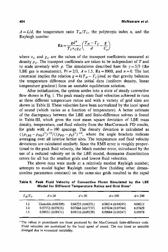
A = L/d, the temperature ratio Tze/Tc, the polytropic index n, and the Rayleigh number

R a = gd4 ( T ~ - T c g ) Tc v c---z c

where v c and Xc are the values of the transport coefficients measured at density p c. The transport coefficients are taken to be independent of T and to scale inversely with p. The simulations described here fix y = 5/3 (the LBE gas is monatomic), Pr = 2/3, A = 1.5, Ra = 8000, and n =0. The last constraint implies the relation g = k( T H - Tc)/md, so that gravity balances the temperature difference and the initial data (uniform density, linear temperature gradient) form an unstable equilibrium solution.

After initialization, the system settles into a state of steady convective flow shown in Fig. 1. The peak steady-state fluid velocities achieved in runs at three different temperature ratios and with a variety of grid sizes are shown in Table II. These velocities have been normalized by the local speed of sound (which varies as a function of temperature). A better estimate of the discrepancy between the LBE and finite-difference solvers is found in Table III, which gives the root mean square deviation of LBE mass density, temperature, and fluid velocity from the MacCormack FD results, for grids with d = 100 spacings. The density deviation is calculated as ((ffLBE -- ffFD) 2) I/2/( (ffFD -- p0)2) 1/2, where the angle brackets indicate averaging over all interior lattice sites. The temperature and fluid velocity deviations are calculated similarly. Since the RMS error is roughly proportional to the peak fluid velocity, the Mach number error, introduced by the use of a reduced velocity set in the LBE model, dominates discretization errors for all but the smallest grids and lowest fluid velocities.

The above runs were made at a relatively modest Rayleigh number; attempts to model higher Rayleigh number flow (holding other dimensionless parameters constant) on the same-size grids resulted in the rapid

Table II. Peak Fluid Velocity of Convective Flows Simulated by the LBE Model for Different Temperature Ratios and Grid Sizes a

Tn/T c d=24 d=50 d= 100 d=200

1.2 Unstable(0.04109) 0.04223 (0.04231) 0.04214(0.04245) 0.04212 1.4 0.07572 (0.07635) 0.07664 (0.07737) 0.07634 (0.07744) 0.07629 1.5 0.09031 (0.09131) 0.09116 (0.09239) 0.09084 (0.09247) 0.09078

The values in parentheses are those produced by the MacCormack finite-difference code. Fluid velocities are normalized by the local speed of sound. The run listed as unstable diverged due to numerical instability.


t f l t , . . ' ' ~ t 1 I l l ' " . , ~ l l l J i l l ~ [ [ J J ] J I l I l l �9 :~ ; ; . , vv

, . . . . . �9 . . . . . , , ,

(o)

(b)

- . , ~ ' ' ? ~ I ( ( ( , ' / ,

(~)

Fig. 1. Velocity field, vorticity contours, and density contours ~ r flow at R a = 8 0 0 0 and ~ / T c = 1.4 computed on a 300 x 200 grid. Vortici~ is measured in units of vc/d ~, and density in units of P0, the mean density.

Table III. Normalized RMS Deviation for Density, Temperature, and Velocity Between LBE ( d = 100) and MacCormack Simulation Results

for Different Temperature Ratios

TH/Tc Density Temperature Velocity

1.2 0.0182 0.0193 0.0084 1.4 0.0321 0.0345 0.0147 1.5 0.0378 0.0406 0.0172

406 M c N a m a r a et at,

Table IV, Peak Normalized Fluid Velocity as a Function of Rayleigh Number and Lax-Wendrof f Time Step a

Ra 6t = 1.00 6t = 0.99 6t = 0.95 6t = 0.90 ~t = 0.80 MacCormack

8,000 0.0914 0.0916 0.0926 0.0935 0.0944 0.0925 16,000 0.1497 0.1500 0.1513 0.1527 0.1540 0.1518 32,000 Unstable 0.2272 0.2291 0.2310 0.2326 0.2295 64,000 Unstable Uns tab le Unstable 0.3259 0.3287 0.3247

" Runs listed as unstable diverged due to numerical instability. The last column gives peak normalized fluid velocity obtained from the MacCormack solver on a 150 x 100 grid.

onset of numerical instability as the t ransport coefficients were decreased.

The Lax-Wendro f f advect ion scheme overcomes this instability at the cost

of introducing some numerical diffusion into the simulation. To determine

how far the Rayleigh number might be increased, and at what cost in terms

of lost accuracy, a series of simulations was run on 75 x 50 grids with

T H / T c = 1.5 at Rayleigh numbers of 8000-64,000 using Lax -Wendro f f t ime

steps ranging from 1 to 0.80. Table IV shows the peak normalized fluid

velocity attained for these runs together with similar results from the MacCormack solver. Table V shows the RMS deviat ion for normalized fluid

velocity between the LBE Lax-Wendro f f results and the M a c C o r m a c k

comparison runs. As expected, the error generally increases with decreasing

time step; however, the Mach number error is usually larger than the

numerical viscosity error. Fur thermore , the highest Rayleigh number

simulations are numerically unstable unless Lax -Wendro f f advection is used.

Table V. R M S Error in Normal ized Fluid Velocity Between the LBE Lax-Wendrof f Runs and the 150x 100 MacCormack Simulations a

Ra 6t = 1.00 6t = 0.99 6t = 0.95 6t = 0.90 6t = 0.80

8,000 0.0174 0.0180 0.0227 0.0296 0.0360 16,000 0.0327 0.0334 0.0365 0.0406 0.0428 32,000 Unstable 0.0560 0.0587 0.0615 0.0605 64,000 Unstable Unstable Unstable 0.0880 0.0850

Runs listed as unstable diverged due to numerical instability.


4. C O N C L U S I O N S

This paper describes a three-dimensional multispeed thermal LBE model that uses 21 speeds on a cubic lattice. The collision operator in the model contains two relaxation times to separately control viscosity and thermal diffusion. A good agreement (within a few percent) is found when comparing this model with a conventional explicit finite-difference Navier- Stokes solver in modeling compressible Rayleigh-B~nard convective flows with Mach number less than 0.1. The Lax-Wendroff advection operator permits the LBE model to operate over a substantially wider range of Rayleigh number at a small computational cost and with modest numerical error.

The earlier nonthermal LBE models were found to have greater numerical stability than thermal LBE models. For example, in simulations of the Kelvin-Helmholtz instability at high Reynolds number (i.e., low viscosity), a nonthermal LBE model was at least as stable as conventional CFD calculationsJ'-~ This resulting stability is presumably a fortunate cir- cumstance, given that the advection was at the Courant limit. Preliminary work indicates that while Lax-Wendroff does increase the stability of nonthermal models somewhat, the resulting numerical viscosity exceeds the already low physical viscosity, causing an unacceptable loss of accuracy. The different stability properties of thermal and nonthermal models and the subsequent utility of advection schemes such as Lax-Wendroff for these models merit further study.

Considering that the LBE model took comparable computer time to the explicit finite-difference MacCormack calculation, that similar stabilization procedures must be invoked, that the boundary conditions are treated analogously, and that adaptive mesh procedures are difficult to implement in LBE, 1221 we have not yet discovered an advantage to employing LBE over conventional Navier-Stokes solvers for thermal systems.

A C K N O W L E D G M E N T S

The authors wish to thank F. Alexander for helpful discussions. This work was performed under the auspices of the U.S. Department of Energy at the Los Alamos National Laboratory and the Lawrence Livermore National Laboratory under contract no. W-7405-Eng-48.

REFERENCES

1. U. Frisch, B. Hasslacher, and Y. Pomeau, Lattice gas automata for the Navier-Stokes equation, Phys. Rev. Lett. 56:1505 (1986).

2. U. Frisch, D. d'Humi+res, B. Hasslacher, P. Lallemand, Y. Pomeau, and J.-P. Rivet, Lattice gas hydrodynamics in two and three dimensions, Complex Systems 1:649 (1987).

408 McNamara et al.

3. S. Chen, M. Lee, K. H. Zhao, and G. D. Doolen, A lattice gas model with temperature, Physica D 37:42 (1989).

4. S. Y. Chen, H. D. Chert, G. D. Doolen, S. Gutman, and M. Lee, A lattice gas model for thermohydrodynamics, J. Star. Phys. 62:1121 (1991).

5. G. McNamara and G. Zanetti, Use of the Boltzmann equation to simulate lattice-gas automata, Phys. Rev. Left. 61:2332 (1988).

6. F. J. Higuera and J. Jimenez, Boltzmann approach to lattice gas simulations, Europhys. Lett. 9:663 (1989).

7. F. J. Higuera, S. Succi, and R. Benzi, Lattice gas dynamics with enhanced collisions, Europhys. Lett. 9:345 (1989).

8. A. Bartoloni, C. Battista, S. Cabasino, P. S. Paolucci, J. Pech, R. Sarno, G. M. Todesco, M. Torelli, W. Tross, P. Vicini, R. Benzi, N. Cabibbo, F. Massaioli, and R. Tripiccione, LBE simulations of Rayleigh-B6nard convection on the APEI00 parallel processor, Int. J. Mod. Phys. C 4:993 (1993).

9. F. J. Alexander, S. Chen, and J. D. Sterling, Lattice Boltzmann thermohydrodynamics, Phys. Rev. E 47:2249 (1993).

I0. Y. Chen, H. Ohashi, and M. Akiyama, Thermal lattice Bhatnagar-Gross-Krook model without nonlinear deviations in macrodynamic equations, Phys. Bey. E 50:2776 (1994).

I1. G. R. McNamara and B. Alder, Analysis of the lattice Boltzmann treatment of hydrodynamics, Physica A 194:218 (1993).

12. Y. H. Qian, D. d'Humi~res, and P. Lallemand, Lattice BGK models for Navier-Stokes equation, Europhys. Lett. 17:479 (1992).

13. S. Chen, Z. Wang, X. Shan, and G. D. Doolen, Lattice Boltzmann computational fluid dynamics in three dimensions, J. Stat. Phys. 68:379 (1992).

14. R. Cornubert, D. d'Humi~res, and D. Levermore, A Knudsen layer theory for lattice gases, Physica D 47:241 (1991).

15. I. Ginzbourg and P. M. Adler, Boundary flow condition analysis for the three-dimensional lattice Boltzmann model, J. Phys. H France 4:191 (1994).

16. D. P. Ziegler, Boundary conditions for lattice Boltzmann simulations, J. Stat. Phys. 71:1171 (1993).

17. P. A. Skordos, Initial and boundary conditions for the lattice Boltzmann method, Phys. Rev. E 48:4823 (1993).

18. F. J. Higuera, Lattice gas method based on the Chapman-Enskog expansion, Phys. Fluids A 2:1049 (1990).

19. A. L. Garcia, Numerical Methods for Physics (Prentice-Hall, Englewood Cliffs, New Jersey, 1994), Chapter 6.

20. S. Gauthier, A spectral collocation method for two-dimensional compressible convection, J. Comput. Phys. 75:217 (1988).

21. G. McNamara and B. Alder, In Microscopic Simulations of Complex Hydrodynamic Phenomena, M. Mareschal and B. L. Holian, eds. (Plenum Press, New York, 1992).

22. R. Benzi, S. Succi, and M. Vergassola, The lattice Boltzmann equation: Theory and applications, Phys. Rep. 222:145 (1992).

Stabilization of thermal lattice Boltzmann models

Documents

Transcript of Stabilization of thermal lattice Boltzmann models